Non-unitarity or hidden observables?

Abstract

A free hermitian conformal field theory is considered in Minkowski, de Sitter and anti-de Sitter spacetimes. The first part of the paper studies spacetime inversion and conformal inversion, wherein their role in the field quantization is elucidated in those spaces. The second part of the paper is concerned with the non-unitary evolution of detector’s state. Several examples of such processes are provided with a clarification of how the unitarity is preserved with still having well-known thermal effects.

I Introduction

Among symmetries of the maximally symmetric spacetimes there are those which are not generated by the algebra of the conformal Killing vectors $L_{AB}\in\mathfrak{so}(2,4)$. These discrete symmetries play a significant role in the quantum theory. In particular, the spacetime inversion $\mathfrak{I}$ in Minkowski space and the charge conjugation appear in the CPT theorem Streater&Wightman .

The inversion $\mathfrak{I}$ appears also as the modular conjugation operator in the Tomita-Takesaki theorem with the modular Hamiltonian represented by the dilatation $D\equiv L_{45}$ Haag . In other words, it turns out the local algebra of observables $\mathcal{A}$ generated by free and real conformal quantum scalar field can be effectively separated into mutually independent (commuting) subalgebras $\mathcal{A}_{\text{I}}$ and $\mathcal{A}_{\text{II}}$, such that $\mathfrak{I}\mathcal{A}_{\text{I,II}}\mathfrak{I}=\mathcal{A}_{\text{II,I}}$ and dynamics in $\mathcal{A}_{\text{I,II}}$ is set by the dilatation $D$. More known example of such a separation of the local observables is given by expanding the field into the left and right Rindler modes, i.e. $\mathcal{A}=\mathcal{A}_{\text{L}}\otimes\mathcal{A}_{\text{R}}$ with the modular conjugation $e^{i\pi\hat{L}_{12}}\circ\mathfrak{I}$ and the modular Hamiltonian given by the boost Lorentz operator $B\equiv L_{03}$. From the physical point of view, it appears that observables composed of the half of the field degrees of freedom satisfy the Kubo-Martin-Schwinger (KMS) condition Haag in the ordinary Poincaré-invariant vacuum $|\Omega\rangle$. That is if $\hat{O}(x)\in\mathcal{A}_{\text{R}}$, then

$$\langle\Omega|\hat{O}(x)|\Omega\rangle = \text{Tr}\big{(}\rho_{\text{T}_{\text{U}}}\hat{O}(x)\big{)}\,,$$ (1)

where $\rho_{\text{T}_{\text{U}}}$ is the density matrix corresponding to the thermal equilibrium at the Unruh (U) temperature $\text{T}_{\text{U}}$ Unruh ; Sciama&Candelas&Deutsch ; Takagi ; Sewell ; Kay . In other words, the pure state $|\Omega\rangle$ appears as a thermal state when one probes it by local observables composed of the specific half of the field degrees of freedom.

In Section II, I will discuss the free and real conformal field quantization in Minkowski, de Sitter (dS) and anti-de Sitter (AdS) spaces. It will turn out that the anti-unitary operator $\mathfrak{I}$ is also a modular conjugation in AdS space and up to a certain unitary operator in dS space for local subalgebras analogous to $\mathcal{A}_{\text{I,II}}$. Besides, I will consider the so-called conformal inversion operator $\mathfrak{I}_{\text{C}}$ and its representation on the solution space $\mathcal{S}$ of the conformal field equation. This operator is unitary and hermitian on $\mathcal{S}$ Kastrup and it will be shown that $\mathfrak{I}_{\text{C}}$ annihilates $\mathcal{A}_{\text{I,II}}$. I will also obtain its eigenfunctions and identify them with the well-known field modes being eigenfunctions of $H\equiv L_{05}$.

In Section III, I will consider various physical processes where the unitarity is violated. It occurs under the assumption that detector’s state can change during those processes. In particular, if one imagines a detector that being inertial starts to speed up till a constant proper acceleration, then its state has to change from the ordinary state to the unitary inequivalent one in order to absorb Rindler particles. This implies a violation of the unitarity. However, the unitarity is preserved if one leaves the state unchanged and admits that the space of observables being felt by the detector alters itself in such a way that some of them become unmeasurable or hidden. That is a local observable $\hat{O}(x)$ being used to probe properties of a quantum state and belonging initially to $\mathcal{A}_{\text{L}}\otimes\mathcal{A}_{\text{R}}$ starts to lie, say, in $\mathbf{\hat{1}}\otimes\mathcal{A}_{\text{R}}$ at some moment of time. I will also discuss how that may perhaps resolve the black hole information paradox Hawking ; Frolov&Novikov ; Brustein .

Throughout this paper the fundamental constants are set to unity, i.e. $c=k_{\text{B}}=G=\hbar=1$ by definition.

II Linear CFT and $\mathfrak{I}$ and $\mathfrak{I}_{\text{C}}$ symmetries

Quantization of a non-interacting field consists of several steps. One of them is to find a classical solution of the field equation. The solution space $\mathcal{S}$ is not positive definite with respect to the Klein-Gordon scalar product taken over Cauchy surface $\Sigma$. However, that space can be divided into two mutually orthogonal subspaces, i.e. $\mathcal{S}={\mathcal{S}^{+}}\oplus\,\mathcal{S}^{-}$, such that the scalar product is positive (negative) definite on $\mathcal{S}^{+}$($\mathcal{S}^{-}$) Birrell&Davies .

The field equation depends on the spacetime metric. I will deal with only maximally symmetric spacetimes. Their line elements can be written down in the following form

$$ds^{2}=a^{2}(x)\eta_{\mu\nu}dx^{\mu}dx^{\nu}\,,\quad\text{where}\quad a(x)\;=\;\frac{1+|\alpha|}{1-\alpha x^{2}}\,$$ (2)

and $x^{2}\equiv\eta_{\mu\nu}x^{\mu}x^{\nu}$, $\eta_{\mu\nu}$ is the Minkowski metric with mostly minus signs. The advantage of that metric is that it allows to consider simultaneously Minkowski, de Sitter or anti-de Sitter spaces by setting $\alpha=0$, $1$ or $-1$, respectively. In case of de Sitter and anti-de Sitter spaces, one has to map $x^{\mu}$ appearing in the metric to $\bar{x}^{\mu}=\exp(+\frac{\pi}{2}L_{05})x^{\mu}$ and $\tilde{x}^{\mu}=\exp(+\frac{\pi}{2}L_{34})x^{\mu}$ to obtain the standard flat and Poincaré patches, respectively. The $\bar{x}^{0}$ coordinate corresponds to the conformal time in flat dS space with the conformal Killing vector $L_{05}+L_{45}$ generating translation along it. The $\tilde{x}^{0}$ coordinate corresponds to the time in the Poincaré patch of AdS space with the Killing vector $L_{05}+L_{03}$ generating $\tilde{x}^{0}$ translation and $\tilde{x}^{3}$ ranges from the horizon ($\tilde{x}^{3}=\infty$) to the boundary ($\tilde{x}^{3}=0$) of AdS space.

In case of the free conformal field theory, one can then immediately find the normalized mode functions of the dynamical equation:

$$\Phi_{\mathbf{k}}(x) = \frac{1}{(2\pi)^{\frac{3}{2}}}\frac{\exp\left(-ikx\right)}{(2k)^{\frac{1}{2}}a(x)}\;\in\;\mathcal{S}^{+},\quad\Phi_{\mathbf{k}}^{*}(x)\;\in\;\mathcal{S}^{-},$$ (3)

where star denotes the complex conjugation. However, it is convenient to introduce spherical coordinates. This transformation induces a unitary map of the spaces $\mathcal{S}^{\pm}$ into themselves. That unitary operator $S(k,l,m|\mathbf{k})$ equals $i^{l}k^{-1}Y_{lm}^{*}(\Omega_{\mathbf{k}})\delta(k-k^{\prime})$ and provides

$$\Phi_{klm}(x) = \int d^{3}\mathbf{k}^{\prime}\,S^{*}(k,l,m|\mathbf{k}^{\prime})\Phi_{\mathbf{k}^{\prime}}(x)\;=\;\left(\frac{k}{\pi}\right)^{\frac{1}{2}}\frac{\exp\left(-ikx^{0}\right)}{a(x^{0},|\mathbf{x}|)}j_{l}\big{(}k|\mathbf{x}|\big{)}Y_{lm}\big{(}\Omega_{\mathbf{x}}\big{)}\,,$$ (4)

where $k\equiv|\mathbf{k}|\in\mathbb{R}^{+}$. The rescaled modes, i.e. $a(x)\Phi_{klm}(x)$, can be in turn expanded via eigenfunctions of the dilatation operator $D$, i.e. $a(x)\Phi_{plm}(x)$, where $p\in\mathbf{R}$. The unitary operator relating them is $C(p|k)=(2\pi)^{-\frac{1}{2}}k^{-ip-\frac{1}{2}}$ Tanaka&Sasaki :

$$\Phi_{plm}(x) = \int dk\,C^{*}(p|k)\Phi_{klm}(x)$$ (5)

$$= \frac{i^{l}\exp\left(+\frac{\pi i}{4}\right)}{a(x^{0},|\mathbf{x}|)\left(4\pi|\mathbf{x}|\right)^{\frac{1}{2}}}\frac{\Gamma\left(1+l+ip\right)}{\left(|\mathbf{x}|^{2}-(x^{0})^{2}\right)^{\frac{ip}{2}+\frac{1}{4}}}P_{ip-\frac{1}{2}}^{-l-\frac{1}{2}}\left(\frac{ix^{0}}{\left(|\mathbf{x}|^{2}-(x^{0})^{2}\right)^{\frac{1}{2}}}\right)Y_{lm}(\Omega)\,.$$

The dilatation vector $D$ is not globally time- or spacelike, it divides space into subspaces, wherein it is either timelike or spacelike. It means that $\Phi_{plm}(x)$ is a restriction of the ordinary modes $\Phi_{\mathbf{k}}(x)$ defined on whole space into those subspaces. Assuming $D$ is timelike and future-directed (the region I in fig. 1), one has to set $(|\mathbf{x}|^{2}-t^{2})^{\frac{1}{2}}=i(t^{2}-|\mathbf{x}|^{2})^{\frac{1}{2}}$ in (5).

II.1 Representation of $\mathfrak{I}$ and $\mathfrak{I}_{\text{C}}$ on $\mathcal{S}$

Among global symmetries of spacetimes under consideration, it turns out there are two which play a distinguished role in the quantization of the field. Specifically, the inversion $\mathfrak{I}$ and conformal inversion $\mathfrak{I}_{\text{C}}$ defined as

$$\mathfrak{I}x^{\mu} \equiv -x^{\mu}\,\quad\textrm{and}\quad\mathfrak{I}_{\text{C}}x^{\mu}\;\equiv\;-\frac{x^{\mu}}{x^{2}}\,.$$ (6)

These transformations provide a map of spacetime into itself which can also be understood in terms of certain operators mapping $\mathcal{S}$ into itself.

To recover the action of $\mathfrak{I}$ on the modes $\Phi_{plm}(x)$, one has first to consider the operator $\mathfrak{I}\circ\mathfrak{I}_{\text{C}}$. This composite operator is anti-unitary, therefore $\mathfrak{I}\circ\mathfrak{I}_{\text{C}}\Phi_{plm}(x)\in\mathcal{S}^{-}$. This means one can unitary map $\mathfrak{I}\circ\mathfrak{I}_{\text{C}}\Phi_{plm}(x)$ into $\Phi_{plm}^{*}(x)$. Hence, one obtains

$$\mathfrak{I}(p|p^{\prime}) = (-1)^{l+1}\delta(p+p^{\prime})\,\delta_{ll^{\prime}}\delta_{mm^{\prime}}\,\mathfrak{C}\,,$$ (7)

where $\mathfrak{C}$ is the complex conjugation operator. Hence, the operator $\mathfrak{I}$ is an anti-unitary on $\mathcal{S}$, i.e. $\mathfrak{I}\mathcal{S}^{\pm}=\mathcal{S}^{\mp}$.

The conformal inversion $\mathfrak{I}_{\text{C}}$ is represented by a unitary and hermitian operator on the spaces $\mathcal{S}^{\pm}$ Kastrup . Indeed, one has

$$\mathfrak{I}_{\text{C}}(\mathbf{k}|\mathbf{k}^{\prime}) \equiv \big{(}\mathfrak{I}_{\text{C}}\Phi_{\mathbf{k}},\Phi_{\mathbf{k}^{\prime}}\big{)}_{\Sigma}\;=\;-\frac{J_{0}\big{(}(2k^{\mu}k_{\mu}^{\prime})^{\frac{1}{2}}\big{)}}{4\pi\left(kk^{\prime}\right)^{\frac{1}{2}}}\,$$ (8)

and $\big{(}\mathfrak{I}_{\text{C}}\Phi_{\mathbf{k}},\Phi_{\mathbf{k}^{\prime}}^{*}\big{)}_{\Sigma}=0$, where $k\equiv|\mathbf{k}|$. Thus, $\mathfrak{I}_{\text{C}}^{\dagger}(\mathbf{k}|\mathbf{k}^{\prime})=\mathfrak{I}_{\text{C}}(\mathbf{k}|\mathbf{k}^{\prime})$ and

$$\int d\mathbf{k}^{\prime\prime}\,\mathfrak{I}_{\text{C}}^{\dagger}(\mathbf{k}|\mathbf{k}^{\prime\prime})\mathfrak{I}_{\text{C}}(\mathbf{k}^{\prime\prime}|\mathbf{k}^{\prime}) = \delta\big{(}\mathbf{k}-\mathbf{k}^{\prime}\big{)}\,.$$ (9)

The operator $\mathfrak{I}_{\text{C}}(\mathbf{k}|\mathbf{k}^{\prime})$ is an integral transform of the modes $\Phi_{\mathbf{k}}(x)$ into those lying in $\mathcal{S}^{+}$. In the following I will mostly deal with the modes $\Phi_{plm}(x)$ in which $\mathfrak{I}_{\text{C}}(\mathbf{k}|\mathbf{k}^{\prime})$ represented as

$$\mathfrak{I}_{\text{C}}(p|p^{\prime}) = \int dkdk^{\prime}d\mathbf{q}d\mathbf{q}^{\prime}C^{*}(p|k)S^{*}(k|\mathbf{q})\mathfrak{I}_{\text{C}}(\mathbf{q},\mathbf{q}^{\prime})C(p^{\prime}|k^{\prime})S(k^{\prime}|\mathbf{q}^{\prime})$$ (10)

$$= -\frac{\Gamma\left(1+l+ip\right)}{\Gamma\left(1+l-ip\right)}\,\delta(p+p^{\prime})\,\delta_{ll^{\prime}}\delta_{mm^{\prime}}\,,$$

where $\{l,m\}$ and $\{l^{\prime},m^{\prime}\}$ parameters have been suppressed. Since the unitary and hermitian operator $\mathfrak{I}_{\text{C}}$ acts on the manifolds as a transformation of I into II and vice versa, the modes in II equivalent to $\Phi_{plm}(x)$ in I are given by $\mathfrak{I}_{\text{C}}\Phi_{plm}(x)$.

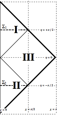
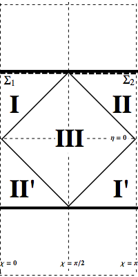
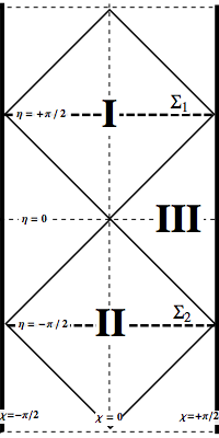
Figure 1: Conformal or Penrose diagrams of Minkowski (left), de Sitter (middle) and anti-de Sitter (right) spacetimes embedded in the Einstein static universe. The coordinates $(\eta,\chi,\theta,\phi)$ are the so-called closed coordinates in which the spatial section has a topology $\mathbf{S}^{3}$. Each point on the plots is a two-dimensional sphere with the coordinates $(\theta,\phi)$.

Introducing the so-called open coordinates $x^{0}=e^{\bar{\eta}}\cosh\bar{\chi}$ and $|\mathbf{x}|=e^{\bar{\eta}}\sinh\bar{\chi}$ (see App. A) in $\Phi_{plm}(x)$ given by (5) and $\mathfrak{I}_{\text{C}}\Phi_{plm}(x)$, one obtains

$$\Phi_{plm}(x) = +\frac{i^{l}e^{+\frac{\pi p}{2}}}{a(\bar{\eta},\bar{\chi})}e^{-ip\bar{\eta}}\frac{\Gamma\left(1+l+ip\right)}{\left(4\pi\sinh\bar{\chi}\right)^{\frac{1}{2}}}P_{ip-\frac{1}{2}}^{-l-\frac{1}{2}}\big{(}\cosh\bar{\chi}\big{)}Y_{lm}(\bar{\Omega})\,,$$ (11a)

$$\mathfrak{I}_{\text{C}}\Phi_{plm}(x) = -\frac{i^{l}e^{-\frac{\pi p}{2}}}{a(\bar{\eta},\bar{\chi})}e^{+ip\bar{\eta}}\frac{\Gamma\left(1+l+ip\right)}{\left(4\pi\sinh\bar{\chi}\right)^{\frac{1}{2}}}P_{ip-\frac{1}{2}}^{-l-\frac{1}{2}}\big{(}\cosh\bar{\chi}\big{)}Y_{lm}(\bar{\Omega})\,.$$ (11b)

The effective Cauchy surface $\Sigma_{\text{eff}}=\Sigma_{1}\cup\Sigma_{2}$ depicted in fig. 1 is enough to set well-defined Cauchy problem. The modes $\Phi_{plm}(x)$ are normalized over it in the following sense

$$(\Phi_{plm},\Phi_{p^{\prime}l^{\prime}m^{\prime}})_{\Sigma_{\text{eff}}} = (\Phi_{plm},\Phi_{p^{\prime}l^{\prime}m^{\prime}})_{\Sigma_{1}}+(\mathfrak{I}_{\text{C}}\Phi_{plm},\mathfrak{I}_{\text{C}}\Phi_{p^{\prime}l^{\prime}m^{\prime}})_{\Sigma_{2}}\;=\;\delta(p-p^{\prime})\delta_{ll^{\prime}}\delta_{mm^{\prime}}\,.$$ (12)

II.2 Continuation of CFT from $\mathbf{R}\times\mathbf{H}^{3}$ to $\mathbf{R}\times\mathbf{S}^{3}$

Since $\mathfrak{I}_{\text{C}}$ is unitary and hermitian, it possesses two eigenvalues $\pm 1$. In other words, the space $\mathcal{S}^{+}$ can be splitted into two orthogonal subspaces $\mathcal{S}_{+}^{+}$ and $\mathcal{S}_{-}^{+}$ Kastrup . The modes $\Phi_{plm}(x)\in\mathcal{S}^{+}$ can be mapped into $\mathcal{S}_{\pm}^{+}$ by applying the projector $\mathbf{P}_{\pm}\equiv\frac{1}{2}(\mathbf{1}\pm\mathfrak{I}_{\text{C}})$. Indeed, with the aid of (10) one gets

$$\mathfrak{I}_{\text{C}}\big{(}\mathbf{P}_{\pm}\Phi_{plm}\big{)} = \pm\mathbf{P}_{\pm}\Phi_{plm}\,.$$ (13)

On the other hand, the operator $\mathfrak{I}_{\text{C}}$ is an integral transform and there exists $M(n|p)$, such that $\mathfrak{I}_{\text{C}}\text{M}(n|p)=(-1)^{n+1}\text{M}(n|p)$, where $n$ is a nonnegative integer (see App.B). Its normalized eigenfunctions are

$$\text{M}(n,p) = \frac{2^{l+1}i^{n+l}}{\Gamma\left(2+2l+n\right)^{\frac{1}{2}}}\frac{\Gamma\left(1+l+n-ip\right)}{(2\pi)^{\frac{1}{2}}\Gamma\left(1+n\right)^{\frac{1}{2}}}$$ (14)

$$\times\;\frac{\Gamma\left(1+l+ip\right)}{\Gamma\left(1+l-ip\right)}\;_{2}F_{1}\left(-n,1+l+ip,-n-l+ip;-1\right)\,.$$

Thus, one can define modes $\Phi_{nlm}(x)$ labeled by the discrete parameter $n$ ($\geq 0$) instead the continuous one $p$ ($\in\mathbf{R}$) as follows

$$\Phi_{nlm}(x) = \int dp\;\text{M}^{*}(n|p)\Phi_{plm}(x)\,,$$ (15)

such that $\mathfrak{I}_{\text{C}}\Phi_{nlm}(x)=(-1)^{n+1}\Phi_{nlm}(x)$. Taking into account the action of $\mathfrak{I}_{\text{C}}$ on spacetime points, one can establish that $a(x)\Phi_{nlm}(x)$ are eigenfunctions of the Killing vector $H$ (see App. C):

$$\Phi_{nlm}(x) = \frac{i^{n+l+1}\sin^{l}\chi}{2^{l+1}a(\eta,\chi)}\frac{\Gamma\left(2+2l\right)\Gamma\left(1+n\right)^{\frac{1}{2}}}{\Gamma\left(l+\frac{3}{2}\right)\Gamma\left(2+2l+n\right)^{\frac{1}{2}}}e^{-i(n+l+1)\eta}C_{n}^{l+1}(\cos\chi)Y_{lm}(\Omega)\,$$ (16)

expressed in the so-called closed coordinates (see App. A).

Thus, the modes $\Phi_{plm}(x)$ found in spacetime with the hyperbolic spatial section $\mathbf{H}^{3}$ have been related with those defined on the spherical one $\mathbf{S}^{3}$. Therefore, $\Phi_{plm}(x)$ can be continued to whole spacetime and, hence, to the Einstein static universe Luescher&Mack .

II.3 Thermal states

For an observer freely moving through the region I and having no excess to the region II, the ordinary CFT vacuum is seen as filled with the thermal bath of particles defined with respect to $D$. Rigorously speaking, the CFT vacuum restricted to the region I is a conformal KMS state with temperature $\text{T}=1/2\pi a(\bar{\eta})$.

Minkowski space

The region I in Minkowski space is identified with the expanding Milne universe. The dilatation operator $D$ is a generator of comoving geodesics in that region. Its positive frequency eigenfunctions define the so-called conformal Milne vacuum. The Minkowksi and Milne vacua are not unitary equivalent. An observer probing the quantum field being in the Minkowski state has to find it as being a thermal state with temperature $\text{T}=e^{-\bar{\eta}}/2\pi$, where $e^{2\bar{\eta}}=x^{2}\in(0,+\infty)$ Birrell&Davies .

The region III in fig.1 is Rindler spacetime to be associated with the proper reference frame of a uniformly accelerated observer in Minkowski space. Dynamics in the Rindler frame is governed by the boost Killing vector $B$ whose positive frequency eigenfunctions define the Rindler vacuum. It is unitary equivalent to the Milne vacuum Hislop&Longo . Indeed, the region I in the open coordinates $(\bar{\eta},\bar{\chi},\bar{\theta},\bar{\phi})$ is mapped into III by

$$e^{\bar{\phi}L_{12}-\bar{\theta}L_{13}}\,e^{\frac{\pi}{2}L_{05}-\frac{\pi}{2}L_{34}}\,e^{\bar{\theta}L_{13}-\bar{\phi}L_{12}}$$ (17)

which has a unitary implementation providing isomorphism between $\mathcal{A}_{\text{I}}$ and $\mathcal{A}_{\text{R}}$.

This transformation can be understood as $\bar{\eta}\rightarrow\tilde{\chi}-\frac{\pi i}{2}$, $\bar{\chi}\rightarrow\tilde{\eta}+\frac{\pi i}{2}$, $\bar{\theta}\rightarrow\tilde{\theta}$ and $\bar{\phi}\rightarrow\tilde{\phi}$, so that $\text{T}=e^{-\bar{\eta}}/2\pi\rightarrow e^{-\tilde{\chi}+\frac{\pi i}{2}}/2\pi i=e^{-\tilde{\chi}}/2\pi$, where the new coordinates $(\tilde{\eta},\tilde{\chi},\tilde{\theta},\tilde{\phi})$ cover Rindler space with the line element taking the following form

$$ds^{2} = e^{2\tilde{\chi}}\big{(}d\tilde{\eta}^{2}-d\tilde{\chi}^{2}-\cosh^{2}\tilde{\eta}\,d\tilde{\Omega}^{2}\big{)}\,.$$ (18)

One can associate an acceleration $a^{\mu}$ to a timelike Killing vector $K^{\mu}$ as follows

$$a^{\mu} = \frac{\nabla_{K}K^{\mu}}{K^{2}}\,,$$ (19)

where $\nabla_{K}$ is a covariant derivative along $K^{\mu}$ and $K^{2}=g_{\mu\nu}K^{\mu}K^{\nu}$ Narnhofer&Peter&Thirring . Setting $\tilde{\theta}=0$ without loss of generality, one obtains $|a|\equiv(-g_{\mu\nu}a^{\mu}a^{\nu})^{\frac{1}{2}}=e^{-\tilde{\chi}}$ for $K=B$. Hence, one obtains the Unruh temperature $\text{T}_{\text{U}}=|a|/2\pi$ measured by the accelerated observer Unruh .

De Sitter space

The region I is open dS space (spatial section is hyperbolic $\mathbf{H}^{3}$ like in the Milne universe). The comoving geodesics in I are the integral curves of the dilatation $D$. The Chernikov-Tagirov state restricted to it is a thermal state, so that a comoving observer in open de Sitter space has to register a thermal bath of particles defined with respect to $D$ with temperature $\text{T}=-\sinh\bar{\eta}/2\pi$, where now $\bar{\eta}\in(-\infty,0)$.

The region III is associated with the proper reference frame of a geodesic observer ($\chi=\frac{\pi}{2}$) or a uniformly accelerated one ($\chi\neq\frac{\pi}{2}$) in de Sitter spacetime. This is the so-called static de Sitter space. Dynamics inside the region III is set by the Killing vector $B$. The region I is mapped to the region III by (17). Performing the same analytic continuation of $(\bar{\eta},\bar{\chi})$ into $(\tilde{\eta},\tilde{\chi})$ and setting $\tilde{\theta}=0$, one derives the Narnhofer-Peter-Thirring (NPT) temperature $\text{T}_{\text{NPT}}=\cosh{\tilde{\chi}}/2\pi=(|a|+1)^{\frac{1}{2}}/2\pi$ Narnhofer&Peter&Thirring . It diverges on the horizons and reduces to the Gibbons-Hawking (GH) temperature $\text{T}_{\text{GH}}=1/2\pi$ for the geodesic observer Gibbons&Hawking .

Anti-de Sitter space

This case is mostly a repetition of the Minkwoski and de Sitter ones, wherein one takes the AdS state as a physical vacuum Avis&Isham&Storey . The value of temperature merely changes due to the difference between scale factors of the spaces (2) and equals $\cosh\bar{\eta}/2\pi$ in the region I of AdS space, where $\bar{\eta}\in(-\infty,+\infty)$ Emelyanov .

The region III is filled by the integral curves of $B$ associated with the observer moving with a constant acceleration. Performing the analytic continuation of the coordinates $(\bar{\eta},\bar{\chi})$ as above, one obtains the Deser-Levin (DL) temperature $\text{T}_{\text{DL}}=\sinh\tilde{\chi}/2\pi=(|a|^{2}-1)^{\frac{1}{2}}/2\pi$ registered by the uniformly accelerated detector Deser&Levin . The AdS horizons and boundary are at $\tilde{\chi}=+\infty$ and $\tilde{\chi}=0$, respectively. Thus, temperature $\text{T}_{\text{DL}}$ is divergent on the horizons and vanishes on the boundary.

One can now straightforwardly generalize the results found in Minkowski space in Hislop&Longo to de Sitter and anti-de Sitter spaces for the free conformal field theory. Specifically, the conformal vacuum defined in the region I of the dS (AdS) hyperboloid is unitary equivalent to the vacuum state defined in the region III of dS (AdS) space.

II.4 Operators $\mathfrak{I}$ and $\mathfrak{I}_{\text{C}}$ and inequivalent quantization

The modes defining the conformal vacua in the regions I and II and normalized over $\Sigma_{1}$ and $\Sigma_{2}$ in Minkowski spacetime are

$$\Phi_{\omega lm}^{\text{I}}(x) = \frac{\exp\left(+\frac{\pi\omega}{2}\right)}{\left(2\sinh\pi\omega\right)^{\frac{1}{2}}}\big{(}\Phi_{+\omega lm}(x)-(-1)^{l}e^{-\pi\omega}\Phi_{-\omega lm}^{*}(x)\big{)}\,,$$ (20a)

$$\Phi_{\omega lm}^{\text{II}}(x) = \frac{\exp\left(+\frac{\pi\omega}{2}\right)}{\left(2\sinh\pi\omega\right)^{\frac{1}{2}}}\big{(}\Phi_{-\omega lm}^{*}(x)-(-1)^{l}e^{-\pi\omega}\Phi_{+\omega lm}(x)\big{)}\,,$$ (20b)

where $\omega\equiv|p|$. According to the Tomita-Takesaki theorem specialized to the present case Haag , $\mathfrak{I}$ is the modular conjugation operator. In particular, it means that $\mathfrak{I}$ maps $\Phi_{\omega lm}^{\text{I}}(x)$ into $\Phi_{\omega lm}^{\text{II}}(x)$ and vice versa:

$$\mathfrak{I}\Phi_{\omega lm}^{\text{I}}(x) = \Phi_{\omega lm}^{\text{II}}(x)\,\quad\textrm{and}\quad\mathfrak{I}_{\text{C}}\Phi_{\omega lm}^{\text{II}}(x)\;=\;\Phi_{\omega lm}^{\text{I}}(x)\,.$$ (21)

Since $\Phi_{\omega lm}^{\text{I}}(x)$ and $\Phi_{\omega lm}^{\text{II}}(x)$ have zero supports in regions II and I, respectively, they must be, however, annihilated by the operator $\mathfrak{I}_{\text{C}}$. Indeed, using (10), one obtains

$$\mathfrak{I}_{\text{C}}\Phi_{\omega lm}^{\text{I}}(x) = 0\,\quad\textrm{and}\quad\mathfrak{I}_{\text{C}}\Phi_{\omega lm}^{\text{II}}(x)\;=\;0\,.$$ (22)

These results can be immediately generalized to dS and AdS spaces. The action of the operators $\mathfrak{I}$ and $\mathfrak{I}_{\text{C}}$ do not change on the space $\mathcal{S}$. However, its action on the spacetime points slightly differs in dS and AdS spaces from that in Minkowski one. In terms of the closed coordinates $(\eta,\chi,\theta,\phi)$ (see App. A) covering the whole spaces under consideration, one finds

$$\mathfrak{I}(\eta,\chi,\theta,\phi) = \left\{\begin{array}[]{cl}(-\eta,\chi,\pi-\theta,\pi+\phi)&\text{-- de Sitter space}\,,\\[2.84526pt] (2\pi k-\eta,\chi,\pi-\theta,\pi+\phi)&\text{-- anti-de Sitter space}\,,\end{array}\right.$$ (25)

and

$$\mathfrak{I}_{\text{C}}(\eta,\chi,\theta,\phi) = \left\{\begin{array}[]{cl}(\eta,\pi-\chi,\theta,\phi)&\text{-- de Sitter space}\,,\\[2.84526pt] (\eta-\pi+2\pi k,\chi,\pi-\theta,\pi+\phi)&\text{-- anti-de Sitter space}\,,\end{array}\right.$$ (28)

where $k\in\mathbb{Z}$.

De Sitter space

The operator $\mathfrak{I}$ maps I into $\text{II}^{\prime}$. However, the region $\text{II}^{\prime}$ can in turn be mapped to the region II by $e^{\pi H/2}$. This mapping has a unitary implementation on $\mathcal{S}$. In other words, the modes $e^{-i\pi\hat{H}/2}\circ\mathfrak{I}_{\text{C}}\Phi_{plm}(x)$ have a nonzero support in $\text{II}^{\prime}$ and define the CFT vacuum in that region like $\Phi_{plm}(x)$ and $\mathfrak{I}_{\text{C}}\Phi_{plm}(x)$ do that in I and II, respectively.

One can define modes $\Phi_{\omega lm}^{\text{I}}(x)$ and $\Phi_{\omega lm}^{\text{II}}(x)$ being analogous to (20) in Minkowski space and defining the conformal vacua in I and II, respectively. The modular conjugation mapping $\Phi_{\omega lm}^{\text{I,II}}(x)$ into $\Phi_{\omega lm}^{\text{II,I}}(x)$ is given by $e^{i\pi\hat{H}/2}\circ\mathfrak{I}$. The operator $\mathfrak{I}_{\text{C}}$ annihilates both of them.

Anti-de Sitter space

The only difference between the operators $\mathfrak{I}$ and $\mathfrak{I}_{\text{C}}$ in anti-de Sitter and Minkowski spaces is that one has infinitely many wedge regions equivalent to I and II in AdS space. The reason lies in that the topology of the AdS hyperboloid is $\mathbf{S}\times\mathbf{R}^{3}$, where the time coordinate $\eta$ runs over the circle $\mathbf{S}$. This leads to the existence of the closed timelike curves. One usually unwraps $\mathbf{S}$ and deals with its universal covering $\mathbf{R}$ to avoid casual paradoxes, i.e. $\eta\in(-\pi,+\pi)\rightarrow\eta\in(-\infty,+\infty)$. Therefore, one has infinitely many wedge regions equivalent to either I or II from the CFT point of view.

III Non-unitarity and hidden observables

III.1 Violation of unitarity

For a quantization of the field $\Phi(x)$ and the concepts of vacuum and particle the symmetries of spacetime play a crucial role. Nevertheless, one can imagine an observer who moves through spacetime not along a (conformal) Killing vector $K$, but along a certain vector field $V$. This vector $V$ sets dynamics in observer’s reference frame. Since, in general, it is not one of $K$ attributed to spacetime, there is no conserved quantity associated with it. However, if there are time intervals during which $V$ is roughly equal to $K$, there has to appear a conserved quantity (Hamiltonian) approximately equaling to that associated with $K$. During these time intervals, the field excitations are naturally defined by expanding the field through the positive and negative frequency modes of $K$, i.e. $\Phi_{\omega}(x)$ and $\Phi_{\omega}^{*}(x)$, s.t.

$$K\big{(}a(x)\Phi_{\omega}(x)\big{)}\;=\;-i\omega\big{(}a(x)\Phi_{\omega}(x)\big{)}\,,$$ (29)

where $\omega\in\mathbf{R}^{+}$ is interpreted as being the energy of the excitation and the rest of indices counting the field degrees of freedom have been suppressed.

Specifically, one may consider a detector moving along

$$V \rightarrow \left\{\begin{array}[]{ll}B\,,&x^{0}\;\rightarrow\;+\infty\,,\\ P_{0}\,,&x^{0}\;\rightarrow\;-\infty\,,\end{array}\right.$$ (32)

where $B=L_{03}=x^{0}\partial_{x^{3}}+x^{3}\partial_{x^{0}}$ and $P_{0}=L_{05}+L_{04}=\partial_{x^{0}}$. At past-time infinity, the detector has presumably to register no particles, i.e. its state is the ordinary Minkowski vacuum. At future-time infinity, the detector has to register the thermal bath with temperature $\text{T}_{\text{U}}$. The operators $\hat{P}_{0}$ and $\hat{B}$ can be mapped into each other, but one has to use a non-unitary operator for that, namely

$$-ie^{-i\pi\hat{L}_{34}/2}e^{-\pi\hat{D}/2}{:} \hat{P}_{0}\;\rightarrow\;\hat{B}\,.$$ (33)

This case has to be distinguished from that when $V\rightarrow D$ at $x^{0}\rightarrow-\infty$, because $\hat{D}$ can be unitary mapped to $\hat{B}$. This means that if one sets detector’s state at past-time infinity to be the conformal Milne one, then the detector along its movement would measure temperature gradually increasing from $0$ to $\text{T}_{\text{U}}$ with no violation of unitarity.

It is worth mentioning another example illustrating what has been meant. One may imagine a universe evolving from Minkwoski space to de Sitter space. This is realized by taking, for instance, the flat FRW metric with the scale factor $a(\eta)=1-1/\eta$, where $\eta\in(-\infty,0)$ is the conformal time and the de Sitter curvature has been set to unity. One can set that at $|\eta|\gg 1$, a comoving detector is in the Minkowski state becoming the Chernikov-Tagirov one at $\eta$ approaching $0$ (both are the ordinary CFT vacuum here). However, its reference frame at $|\eta|\ll 1$ is restricted to de Sitter space in the static coordinates. That is detector’s state would change non-unitary if it can absorb particles defined with respect to the static dS vacuum (positive energy excitations in static dS space defined with respect to $L_{04}$). The unitarity is not violated if detector’s state at past-time infinity is not the Minkowski state, but the conformal Milne one. Nevertheless, the effect is the same in that sense the detector would measure temperature increasing from $0$ to $\text{T}_{\text{GH}}$:

T $$= \frac{1}{2\pi\big{(}1-\eta\big{)}}\;\rightarrow\;\left\{\begin{array}[]{ll}0\,,&\eta\;\rightarrow-\infty\,,\\[4.2679pt] \frac{1}{2\pi}\,,&\eta\;\rightarrow\;-0\,,\end{array}\right.$$ (36)

assuming the detector is located at the spatial origin. Note that in this case $V\rightarrow D$ at past-time infinity and $V\rightarrow L_{04}$ at future-time infinity. The dilatation $\hat{D}$ and $\hat{L}_{04}$ can be mapped into each other by the unitary operator generated by $\hat{H}$.

It is important to distinguish these cases from particle production in a universe evolving in time $t$. To have particle production, one has explicitly to break the conformal symmetry by adding, for example, a mass term. This results in the time-dependence of the frequency $\omega$. Assuming that $\omega\rightarrow\omega_{\text{in}}=\text{const}$ at past-time infinity and $\omega\rightarrow\omega_{\text{out}}=\text{const}\neq\omega_{\text{in}}$ at future-time infinity, the normalized modes $\Phi_{1}(x)$ solving the field equation and approaching $\Phi_{\text{in}}(x)\propto e^{-i\omega_{\text{in}}t}$ at $t\rightarrow-\infty$ become a linear combination of $\Phi_{\text{out}}(x)$ and $\Phi_{\text{out}}^{*}(x)$ at $t\rightarrow+\infty$, where $\Phi_{\text{out}}(x)\propto e^{-i\omega_{\text{out}}t}$ is obtained from another solution $\Phi_{2}(x)$ of the field equation at that limit. The map between $\{\Phi_{1}(x),\Phi_{1}^{*}(x)\}$ and $\{\Phi_{2}(x),\Phi_{2}^{*}(x)\}$ is perfectly unitary and known as the squeezed transformation. Note that this process is similar to the Schwinger effect, i.e. the $\text{e}^{+}\text{e}^{-}$ pair production by the static electric field (see, for example, Anderson&Mottola and references therein).

To sum it up, if detector’s state can vary between the Minkowski and the thermal states, then one encounters a violation of the unitarity.

III.2 Hidden field degrees of freedom

To preserve the unitarity one may admit that detector’s state can be identified with the thermal state (non-CFT vacuum). I will discuss below another possibility, i.e. whether its state identified with CFT one could stay unchanged with still measuring well-known thermal effects.

Inertial detector

Consider an inertial detector $\mathbf{D}_{1}$ which internal dynamics is set to be governed by

$$V_{1} = \left\{\begin{array}[]{lcll}P_{0}\,,&|x^{0}|&\geq&1\,,\\[2.84526pt] R\,,&|x^{0}|&<&1\,,\end{array}\right.$$ (39)

where $R\equiv L_{04}$. The detector $\mathbf{D}_{1}$ is not excited at $|x^{0}|\geq 1$. However, its internal dynamics considerably changes at $x^{0}=\pm 1$, such that the concept of the physical field excitation becomes different during $x^{0}\in(-1,+1)$ from the ordinary one. One can show that its proper reference frame coincides up to a conformal factor with the open FRW universe at $x^{0}\in(-1,+1)$. Hence, one immediately obtains that $\mathbf{D}_{1}$ has to be thermally excited with temperature

$$\textrm{T}_{\mathbf{D}_{1}} = \frac{1/\pi}{1-(x^{0})^{2}}\,,$$ (40)

where it has been assumed the detector is located at the spatial origin Hislop&Longo ; Haag .

The time interval $(-1,+1)$ can be stretched to almost whole Minkowski space. Indeed, the hermitian operator $\hat{R}$ is unitary transformed to the linear combination of $\hat{D}$, $\hat{H}$ and itself as follows

$$\hat{R}^{\,\prime} = \big{(}e^{i\alpha\hat{D}}e^{i\beta\hat{H}}\big{)}\hat{R}\big{(}e^{i\alpha\hat{D}}e^{i\beta\hat{H}}\big{)}^{\dagger}\;=\;\big{(}\hat{R}\cosh\alpha-\hat{H}\sinh\alpha\big{)}\cos\beta-\hat{D}\sin\beta\,,$$ (41)

where $\alpha\in\mathbf{R}$ and $\beta\in[-\frac{\pi}{2},+\frac{\pi}{2}]$. This means, in particular, that one can map $(-1,+1)$ to the expanding or contracting Milne universe (see fig.2) by setting $\beta=-\pi/2$ or $\beta=+\pi/2$, respectively. This combination of operators approaches $\hat{P_{0}}$ in the limit $\alpha\rightarrow-\infty$. In other words, the integral curves of $R^{\,\prime}$ fills out almost the whole space at that limit. If internal dynamics of the detector $\mathbf{D}_{1}$ is now set by $R^{\,\prime}$ given in (41) during $x^{0}\in(x_{\text{i}}^{0},x_{\text{f}}^{0})=(-e^{-\alpha}(\sec\beta+\tan\beta),+e^{-\alpha}(\sec\beta-\tan\beta))$, then it will be thermally excited with the following temperature

$$\text{T}_{\mathbf{D}_{1}} = \frac{1/\pi}{\left(e^{-\alpha}-e^{+\alpha}(x^{0})^{2}\right)\cos\beta-2x^{0}\sin\beta}\,.$$ (42)

At the limit $\alpha\rightarrow-\infty$ and assuming $\beta\neq\pm\pi/2$, $\text{T}_{\mathbf{D}_{1}}$ vanishes at fixed $x^{0}$ strongly inside its range. With no respect of the value of $\alpha$, this temperature is divergent on the boundary values of $x^{0}$.

If one describes this process as a change of detector’s state, then one has a breakdown of the unitarity. Indeed, its state is supposed to be the Minkowski vacuum at $x^{0}\notin(x_{\text{i}}^{0},x_{\text{f}}^{0})$. Inside that time interval, it has to be changed to the nonstandard vacuum with respect to which the nonstandard field excitations have been defined above. Thus, the pure state becomes thermalized. However, one can still have the thermal effect without changing detector’s state and defining a new vacuum. To illustrate this, I will consider below several examples.

The frequency spectrum of the quantum fluctuations being measured by a detector probing all field degrees of freedom can be found by exploiting the formula

$$\mathcal{P}(\omega) = \int\limits_{-\infty}^{+\infty}d\tau\,e^{-i\omega x^{0}(\tau)}\langle\Omega|\hat{\Phi}(x^{0}(\tau))\hat{\Phi}(0)|\Omega\rangle\,,$$ (43)

where $\tau$ is the proper time and $\omega=k$ frequency defined with respect to $x^{0}$ Sciama&Candelas&Deutsch . A geodesic detector $\mathbf{D}_{1}$ being sensitive to all field degrees and moving along $P_{0}$ is not excited by the fluctuations: $\mathcal{P}_{\mathbf{D}_{1}}(\omega)=-\frac{\omega}{2\pi}\,\theta(-\omega)=0$. Suppose a detector $\mathbf{D}_{2}$ is not oblivious only to those field degrees to be defined with respect to $R^{\,\prime}$ inside $(x_{\text{i}}^{0},x_{\text{f}}^{0})$ and moves along $P_{0}$ as well. Its power spectrum is given by

$$\mathcal{P}_{\mathbf{D}_{2}}(\omega) = \int\limits_{-\infty}^{+\infty}d\tau\,e^{-i\omega\bar{\eta}^{\prime}(\tau)}\langle\Omega|\hat{\Phi}(\bar{\eta}^{\prime}(\tau))\hat{\Phi}(0)|\Omega\rangle\,,$$ (44)

where $\omega$ now is the frequency defined with respect to $R^{\,\prime}=\partial/\partial{\bar{\eta}^{\prime}}$. It is not vanishing only during $x^{0}\in(x_{\text{i}}^{0},x_{\text{f}}^{0})$. Evaluating it, one obtains

$$\mathcal{P}_{\mathbf{D}_{2}}(\omega) = 4e^{-\alpha}\cos^{2}(\beta/2)\,\frac{\omega}{e^{2\pi\omega}-1}\,.$$ (45)

Expressing $\omega$ through the physical frequency $\omega_{\text{ph}}$, one finds temperature (42) ascribed to the spectrum. Thus, such a detector would indicate a presence of the thermal bath, although the state has not been changed.

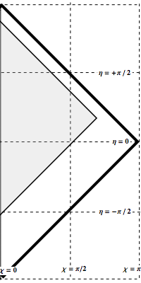
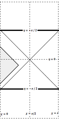
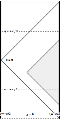
Figure 2: Left: the shaded region in Minkwoski space is filled by the integral curves of $R^{\prime}$. This region can be transformed in the contracting (II depicted in fig.1) or expanding (I depicted in fig.1) Milne universes as well as it can cover almost whole space at $\alpha\rightarrow-\infty$. Middle: the shaded region in dS space is filled also by the curves of $R^{\prime}$ with $\alpha\geq 0$. It can be mapped to open de Sitter by setting $\beta=\mp\frac{\pi}{2}$ (I or $\text{II}^{\prime}$ depicted in fig.1, respectively). Right: the shaded region in the Poincaré patch of AdS space. It is filled by the integral curves of the Killing vector $B^{\,\prime}$ which reduces in particular to the region III depicted in fig.1 if $\alpha=\beta=0$.

Non-inertial detector

The quantum field $\hat{\Phi}(x)$ can be expanded through the ordinary plane waves being the eigenfunctions of $P_{0}$ or, equivalently, through the eigenfunctions of $B$ as follows

$$\hat{\Phi}_{\mathbf{k}}(x) = \int dp\big{(}\hat{\Phi}_{p\mathbf{k}}(x)+\hat{\Phi}_{p\mathbf{k}}^{\dagger}(x)\big{)}\,,\quad B\hat{\Phi}_{p}(x)\;=\;-ip\hat{\Phi}_{p}(x)\,,$$ (46)

where $p\in\mathbf{R}$, $\mathbf{k}=(k_{1},k_{2})$ and $\hat{\Phi}_{p\mathbf{k}}(x)=\Phi_{p\mathbf{k}}(x)\hat{a}_{p}$. One can then introduce $\omega=|p|$ and $\Phi_{\omega\mathbf{k}}^{\text{R}}(x)$ and $\Phi_{\omega\mathbf{k}}^{\text{L}}(x)$ to be positive frequency modes with respect to $B$, such those

$$\Phi_{\omega\mathbf{k}}^{\text{R}}(x) = \alpha_{\omega}\Phi_{+\omega+\mathbf{k}}(x)+\beta_{\omega}\Phi_{-\omega-\mathbf{k}}^{*}(x)\,,$$ (47a)

$$\Phi_{\omega\mathbf{k}}^{\text{L}}(x) = \alpha_{\omega}\Phi_{-\omega+\mathbf{k}}(x)+\beta_{\omega}\Phi_{+\omega-\mathbf{k}}^{*}(x)\,,$$ (47b)

where the Bogolyubov coefficients $\alpha_{\omega}=(1-e^{-2\pi\omega})^{\frac{1}{2}}$ and $\beta_{\omega}=-e^{-\pi\omega}\alpha_{\omega}$. These modes $\Phi_{\omega\mathbf{k}}^{\text{R}}(x)$ and $\Phi_{\omega\mathbf{k}}^{\text{L}}(x)$ vanish in the left and right Rindler wedges, respectively. The field expanded through them takes the following form

$$\hat{\Phi}_{\mathbf{k}}(x) = \int d\omega\big{(}\hat{\Phi}_{\omega\mathbf{k}}^{\text{R}}(x)+\hat{\Phi}_{\omega\mathbf{k}}^{\text{R}\dagger}(x)+\hat{\Phi}_{\omega\mathbf{k}}^{\text{L}}(x)+\hat{\Phi}_{\omega\mathbf{k}}^{\text{L}\dagger}(x)\big{)}\,.$$ (48)

Consider a detector $\mathbf{D}_{3}$ moving along $V$ as in (32), such that it intersects the line $x^{0}=-x^{3}$ at a certain time moment $x^{0}$. According to Davies-Unruh effect, one expects that the modes the detector $\mathbf{D}_{3}$ can in principle probe are given by

$$\Phi_{p\mathbf{k}}^{\text{D}_{3}}(x) = \delta_{+\omega,p}\Phi_{+\omega\mathbf{k}}^{\text{Int}}(x)+\delta_{-\omega,p}\Phi_{-\omega\mathbf{k}}^{\text{Int}}(x)\,,$$ (49)

where delta is the Kronecker symbol and the interpolating modes have to satisfy the following conditions:

$$\Phi_{+\omega\mathbf{k}}^{\text{Int}}(x) = \left\{\begin{array}[]{ll}\alpha_{\omega}\Phi_{\omega+\mathbf{k}}^{\text{R}}(x)-\beta_{\omega}\Phi_{\omega-\mathbf{k}}^{\text{L}*}(x)\,,&x^{0}\;\rightarrow\;-\infty\,,\\[2.84526pt] \Phi_{\omega+\mathbf{k}}^{\text{R}}(x)\,,&x^{0}\;\rightarrow\;+\infty\,,\end{array}\right.$$ (52)

and

$$\Phi_{-\omega\mathbf{k}}^{\text{Int}}(x) = \left\{\begin{array}[]{ll}\alpha_{\omega}\Phi_{\omega+\mathbf{k}}^{\text{L}}(x)-\beta_{\omega}\Phi_{\omega-\mathbf{k}}^{\text{R}*}(x)\,,&x^{0}\;\rightarrow\;-\infty\,,\\[2.84526pt] 0\,,&x^{0}\;\rightarrow\;+\infty\,.\end{array}\right.$$ (55)

The qualitative picture of the process can be described as follows. Initially, at $x^{0}\rightarrow-\infty$, the physical field excitations are the ordinary Minkowski particles, i.e. the detector can feel all field degrees of freedom. However, after having intersected the line $x^{0}=-x^{3}$, the half of them become unavailable to the detector. At future-time infinity, $x^{0}\rightarrow+\infty$, the rest of the degrees can be felt as a new kind of the field excitations, namely the Rindler particles. The definition of a particle implies an introduction of a no-particle state, i.e. vacuum. If detector’s state varies from the Minkowski vacuum to the Rindler state, then one has a violation of the unitarity.

One may assume that detector’s state does not change. However, there are no half of the field degrees of freedom corresponding to the left Rindler modes in the right Rindler wedge. The frequency spectrum of the detector $\mathbf{D}_{3}$ measuring the quantum fluctuations are

$$\mathcal{P}_{\mathbf{D}_{3}}(\omega) = \left\{\begin{array}[]{llll}-\frac{\omega}{2\pi}\,\theta(-\omega)\,,&x^{0}&\rightarrow&-\infty\,,\\[5.69054pt] \frac{2\omega}{\pi|a|}(e^{2\pi\omega}-1)^{-1}\,,&x^{0}&\rightarrow&+\infty\,,\end{array}\right.$$ (58)

where $|a|$ is the acceleration at $x^{0}\rightarrow+\infty$ and it has been assumed that the periods of both inertial and uniformly accelerated motions are sufficiently large to have equality in (58). In terms of the physical frequency $\omega_{\text{ph}}$, one obtains temperature $\text{T}_{\text{U}}$ ascribed to the spectrum at future-time infinity. Although this can be further interpreted as there are some sort of the new (Rindler) particles with the energy $\omega$ which the detector accumulates till reaching the equilibrium stationary state, one has to refrain from such interpretation, otherwise the unitarity is violated.

Suppose one can construct a detector $\mathbf{D}_{4}$ that probes the right Rindler modes $\Phi_{\omega lm}^{\text{R}}(x)$ and is not sensitive to the left ones $\Phi_{\omega lm}^{\text{L}}(x)$. One may now ask a question: What would it measure assuming it moves along $P_{0}$ at $\mathbf{x}=0$? The frequency spectrum of the quantum fluctuation measured by the detector $\mathbf{D}_{4}$ is

$$\mathcal{P}_{\mathbf{D}_{4}}(\omega) = \int\limits_{-\infty}^{+\infty}d\tau\,e^{-i\omega\bar{\eta}(\tau)}\langle\Omega|\hat{\Phi}(\bar{\eta}(\tau))\hat{\Phi}(0)|\Omega\rangle\;=\;\frac{4\omega}{e^{2\pi\omega}-1}\,,$$ (59)

where it has been taken into account that $\Phi_{\omega lm}^{\text{R}}(x)$ can be analytically continued from the region III to the regions I and II. Temperature ascribed to the spectrum is equal to

$$\text{T}_{\mathbf{D}_{4}} = \frac{1}{2\pi|x^{0}|}\,.$$ (60)

This temperature is time-dependent and diverges at $x^{0}=0$. Physically, the detector cannot measure energies higher than a threshold one $E_{\text{c}}$. Therefore, the maximal temperature would be equal to $E_{\text{c}}/2\pi$. Thus, the detector would show a thermal distribution that could be explained without absorption of the Rindler particles, i.e. without changing detector’s state. The detector responses non-trivially to the quantum fluctuation being always present in the vacuum $|\Omega\rangle$ Sciama&Candelas&Deutsch .

De Sitter space

In comparison with Minkowski space, there is a horizon in de Sitter space. A geodesic detector is always oblivious to the half of the field degrees of freedom. The frequency spectrum of the detector is always thermal with the Gibbons-Hawking temperature:

$$\mathcal{P}(\omega) = \int\limits_{-\infty}^{+\infty}dt\,e^{-i\omega t}\langle\Omega|\hat{\Phi}(t)\hat{\Phi}(0)|\Omega\rangle\;=\;\frac{1}{2\pi}\frac{\omega}{e^{2\pi\omega}-1}\,,$$ (61)

where it has been taken into account that $x^{0}=\tanh t$, where $t$ is the physical time Sciama&Candelas&Deutsch .

The observer could define the static vacuum being inequivalent to the Chernikov-Tagirov or Bunch-Davies states Birrell&Davies . This is perfectly fine, if one presumes, however, that the space is eternal. Imagine a universe which is like Minkowski space at past- and future-time infinities and resembles de Sitter space in-between. As above, there are two cases. In the first case, the state of a comoving detector changes and then one has a violation of the unitarity. In the second case, one does not change the state. This detector could still measure the Gibbons-Hawking temperature during the de Sitter space phase for the frequencies $\omega\gtrsim H_{\text{dS}}$ during $H_{\text{dS}}\Delta t\gg 1$, where $\Delta t$ is a physical time interval during which the universe resembles de Sitter space with the curvature $H_{\text{dS}}$. Indeed, the frequency spectrum is

$$\mathcal{P}(\omega) = \int\limits_{-\Delta t/2}^{+\Delta t/2}dt\,e^{-i\omega t}\langle\Omega|\hat{\Phi}(t)\hat{\Phi}(0)|\Omega\rangle$$ (62)

$$= \frac{1}{2\pi}\frac{\omega}{e^{2\pi\omega/H_{\text{dS}}}-1}+\sum_{n=1}^{+\infty}\frac{H_{\text{dS}}n^{2}\cos\left(\omega\Delta t/2\right)-n\omega\sin\left(\omega\Delta t/2\right)}{2\pi^{2}\left(n^{2}+(\omega/H_{\text{dS}})^{2}\right)\exp\left(nH_{\text{dS}}\Delta t/2\right)}\,,$$

where the second term is negligible with respect to the first term under those conditions.

Returning to eternal de Sitter space, one may consider a geodesic detector $\mathbf{D}_{5}$ that is sensitive to the modes defined with respect to $R^{\,\prime}$ during $(x_{\text{i}}^{0},x_{\text{f}}^{0})$ and with $\alpha\geq 0$. Temperature would be

$$\text{T}_{\mathbf{D}_{5}} = \frac{(1-(x^{0})^{2})/2\pi}{\left(e^{-\alpha}-e^{+\alpha}(x^{0})^{2}\right)\cos\beta-2x^{0}\sin\beta}\,.$$ (63)

Note that $\text{T}_{\mathbf{D}_{5}}$ reduces to the Gibbons-Hawking temperature $\text{T}_{\text{GH}}$ when $\beta=0$ and $\alpha=0$. This temperature $\text{T}_{\mathbf{D}_{5}}$ reduces to $-\sinh\bar{\eta}/2\pi$ when $\beta=-\frac{\pi}{2}$ and $\alpha=0$, where $x^{0}=e^{\bar{\eta}}$ at $\mathbf{x}=0$ and $\bar{\eta}\in(-\infty,0)$.

Anti-de Sitter space

An observer moving along $H$ at $\chi=0$ in AdS space is geodesic. Analogously, one may consider a detector $\mathbf{D}_{6}$ that probes merely the half of the field degrees of freedom defined with respect to $R^{\,\prime}$ and measures the frequency spectrum of the quantum fluctuations. Then it would register the thermal distribution with temperature

$$\text{T}_{\mathbf{D}_{6}} = \frac{(1+(x^{0})^{2})/2\pi}{\left(e^{-\alpha}-e^{+\alpha}(x^{0})^{2}\right)\cos\beta-2x^{0}\sin\beta}\,.$$ (64)

If one sets $\beta=-\pi/2$, then this domain of AdS space is the region I in fig. 1, i.e. the so-called open AdS space. The temperature $\text{T}_{\mathbf{D}_{6}}$ reduces to $\cosh\bar{\eta}/2\pi$, where $x^{0}=e^{\bar{\eta}}$ at $\chi=0$.

One can also consider a detector moving along $H+B=\partial/\partial\tilde{x}^{0}$, i.e. the time-translation Killing vector in the Poincaré patch. If this detector is not oblivious to the positive and negative frequency modes defined with respect to

$$\hat{B}^{\,\prime} = \big{(}e^{i\alpha\hat{L}_{35}}e^{i\beta\hat{H}}\big{)}\hat{B}\big{(}e^{i\alpha\hat{L}_{35}}e^{i\beta\hat{H}}\big{)}^{\dagger}\;=\;\big{(}\hat{B}\cosh\alpha+\hat{H}\sinh\alpha\big{)}\cos\beta+\hat{L}_{35}\sin\beta\,.$$ (65)

then temperature of the frequency spectrum is not zero at $\tilde{x}^{3}\neq 0$. This generalizes the result found in Deser&Levin .

III.3 Discussion

I have considered above various examples when the unitarity is violated by allowing a detector to absorb particles which are not defined with respect to the ordinary state $|\Omega\rangle$. The reason is that detector’s state belonging to the ordinary Fock space must non-unitary change to register particles defined with respect to the thermal state. Assuming that detector’s state can be prepared to be equivalent to $|\Omega\rangle$, one can still measure the well-known thermal effects which are due to the quantum fluctuations of the field.

The vacuum activity is also probed by the vacuum expectation value of the energy-momentum tensor of the field $\langle\Omega|\hat{T}_{\nu}^{\mu}(x)|\Omega\rangle$. It is divergent as a result of the distributional nature of the quantum field. After appropriate renormalization, it becomes

$$\langle\Omega|\hat{T}_{\nu}^{\mu}(x)|\Omega\rangle_{\text{ren}} = \frac{|\alpha|}{960\pi^{2}}\,\delta_{\nu}^{\mu}\,.$$ (66)

Hence, it vanishes in Minkowski space and non-zero in dS and AdS spaces Birrell&Davies ; Emelyanov . The readings of the detector in Minkowski spacetime explained in terms of the quantum fluctuations fits well, because (66) is zero, i.e. no new (Rindler) particles are present Sciama&Candelas&Deutsch . Although (66) does not vanish for de Sitter and anti-de Sitter spaces, the same picture can be given as well. Indeed, the right-hand side in (66) is due to the conformal trace anomaly Birrell&Davies . A geodesic observer in anti-de Sitter space does not register any field excitations, but $\langle\Omega|\hat{T}_{\nu}^{\mu}(x)|\Omega\rangle_{\text{ren}}\neq 0$. On the contrary, a geodesic observer in de Sitter space has to register a thermal spectrum with temperature $\text{T}_{\text{GH}}$, wherein $\langle\Omega|\hat{T}_{\nu}^{\mu}(x)|\Omega\rangle_{\text{ren}}$ is the same as in AdS space. Therefore, one may conclude that a term due to the particles is absent in (66) for dS and AdS spaces as for the Minkowski case.

What if one considers the case of the final stage of the collapsing non-rotating matter shell, i.e. the Schwarzschild black hole, in the same way? The initial state $|\text{shell}\rangle$ is a coherent state describing the macroscopic system, i.e. the collapsing shell, composed of particles defined with respect to the ordinary vacuum $|\Omega\rangle$. Suppose during the black hole formation, $|\text{shell}\rangle$ evolves unitary in $|\Omega_{\text{BH}}\rangle$, i.e. the Unruh state Unruh ; Sciama&Candelas&Deutsch ; Frolov&Novikov , and observer’s state is unitary equivalent to it.

From the mathematical point of view, the Hawking effect Hawking2 in the case of an eternal black hole can be described in the analogous way as in the above examples Sewell ; Kay . That is one separates the local algebra of observables in two mutually independent (commuting) subalgebras with dynamics set by the Killing vector $\partial_{t}$, where $t$ is the Schwarzschild time. Probing the Hartle-Hawking state by local observables belonging to the one of those subalgebras, it appears as a thermal state with the Hawking temperature.

In the case of the collapsing shell, a similar separation of the local observables has to be realized after the appearance of the event horizon (like still in a idealized consideration in Dappiaggi&Moretti&Pinamonti ) Emelyanov1 . Thus, the local observables with the help of which one can probe the quantum field alters itself, such that a certain part of the field degrees becomes hidden for the observer. The observer being in the gravitational field of the black hole moves along $\partial_{t}$ and can register the thermal frequency spectrum by a detector Sciama&Candelas&Deutsch ; Fredenhagen&Haag . However, this situation is slightly different from those treated above, because the renormalized $\langle\Omega_{\text{BH}}|\hat{T}_{\nu}^{\mu}(x)|\Omega_{\text{BH}}\rangle$ resembles a thermal radiation with the Hawking temperature at the spatial infinity Frolov&Novikov . On the other hand, $\langle\Omega_{\text{BH}}|\hat{T}_{\nu}^{\mu}(x)|\Omega_{\text{BH}}\rangle$ does not look like as for the thermal radiation for an observer being at the finite distance from the black hole. Moreover, it is finite on the horizon, whereas for the pure radiation it is divergent as a result of the infinite blueshift of the temperature. Thus, this observer could perhaps similarly interpret the readings of his detector as in the case of the transition from Minkowski space to de Sitter space described above.

Appendix A Closed and open coordinates

Closed coordinates:

These coordinates $(\eta,\chi,\theta,\phi)$ are related with $x^{\mu}$ as follows

$$x^{0} = \frac{\sin\eta}{\cos\eta+\cos\chi}\,,$$

$$x^{1} = \frac{\sin\chi}{\cos\eta+\cos\chi}\sin\theta\cos\phi\,,$$ (67)

$$x^{2} = \frac{\sin\chi}{\cos\eta+\cos\chi}\sin\theta\sin\phi\,,$$

$$x^{3} = \frac{\sin\chi}{\cos\eta+\cos\chi}\cos\theta\,,$$

in which the line element (2) has the following form

$$ds^{2}=\frac{\left(1+|\alpha|\right)^{2}}{\left((1-\alpha)\cos\chi+(1+\alpha)\cos\eta\right)^{2}}\big{(}d\eta^{2}-d\chi^{2}-\sin^{2}\chi d\Omega^{2}\big{)}\,.$$ (68)

Open coordinates:

These coordinates $(\bar{\eta},\bar{\chi},\bar{\theta},\bar{\phi})$ are related with $x^{\mu}$ as follows

$$x^{0} = e^{\bar{\eta}}\cosh\bar{\chi}\,,$$

$$x^{1} = e^{\bar{\eta}}\sinh\bar{\chi}\sin\bar{\theta}\cos\bar{\phi}\,,$$ (69)

$$x^{2} = e^{\bar{\eta}}\sinh\bar{\chi}\sin\bar{\theta}\sin\bar{\phi}\,,$$

$$x^{3} = e^{\bar{\eta}}\sinh\bar{\chi}\cos\bar{\theta}\,,$$

in which the line element (2) has the following form

$$ds^{2}=\frac{\left(1+|\alpha|\right)^{2}}{\left((1-\alpha)\cosh\bar{\eta}-(1+\alpha)\sinh\bar{\eta}\right)^{2}}\big{(}d\bar{\eta}^{2}-d\bar{\chi}^{2}-\sinh^{2}\bar{\chi}d\bar{\Omega}^{2}\big{)}\,.$$ (70)

Appendix B Eigenfunctions of $\mathfrak{I}_{\text{C}}$

The scalar product between $\Phi_{\mathbf{k}}(x)$ and $\mathfrak{I}_{\text{C}}\Phi_{\mathbf{k}}(x)=x^{-2}\Phi_{\mathbf{k}}(\mathfrak{I}_{\text{C}}x)$ defines an unitary operator $\mathfrak{I}_{\text{C}}(\mathbf{q}|\mathbf{k})$ on $\mathcal{S}^{+}$, i.e.

$$\mathfrak{I}_{\text{C}}(\mathbf{q}|\mathbf{k}) \equiv (\mathfrak{I}_{\text{C}}\Phi_{\mathbf{q}},\Phi_{\mathbf{k}})\;=\;-i\int d^{3}x\left.\big{(}\mathfrak{I}_{\text{C}}\Phi_{\mathbf{q}}\partial_{0}\Phi_{\mathbf{k}}^{*}-\Phi_{\mathbf{k}}^{*}\partial_{0}\mathfrak{I}_{\text{C}}\Phi_{\mathbf{q}}\big{)}\right|_{x^{0}\;=\;0}$$ (71)

$$= \frac{-1}{(2\pi)^{3}}\frac{1}{2(qk)^{\frac{1}{2}}}\int d\mathbf{x}\left(\frac{k}{\mathbf{x}^{2}}+\frac{q}{\mathbf{x}^{4}}\right)e^{i\mathbf{k}\mathbf{x}-i\frac{\mathbf{q}\mathbf{x}}{\mathbf{x}^{2}}}\;=\;\frac{-1}{4\pi}\frac{1}{(qk)^{\frac{1}{2}}}\,J_{0}\big{(}(2q_{\mu}k^{\mu})^{\frac{1}{2}}\big{)}\,,$$

where $q\equiv|\mathbf{q}|$ and $k\equiv|\mathbf{k}|$ Kastrup .

The operator $\mathfrak{I}_{\text{C}}$ is unitary and hermitian, hence it has two eigenvalues $\pm 1$. The unitary operator that map the modes $\Phi_{klm}(x)$ into the eigenfunctions $\Phi_{nlm}(x)$ of $\mathfrak{I}_{\text{C}}$ is given by

$$E(n|k) = 2^{l+1}e^{-\frac{\pi i}{2}(n+l)}\left(\frac{\Gamma\left(1+n\right)}{\Gamma\left(2+2l+n\right)}\right)^{\frac{1}{2}}k^{l+\frac{1}{2}}e^{-k}L_{n}^{2l+1}(2k)\,,\quad n\;\in\;\mathbb{N}_{0}\,,$$ (72)

such that

$$\Phi_{nlm}(x) = \int dkE^{*}(n|k)\Phi_{klm}(x)\,,$$ (73)

One further obtains

$$\Phi_{nlm}(x) = \int\limits_{-\infty}^{+\infty}dp\;\Phi_{plm}(x)\int\limits_{0}^{+\infty}dk\;E^{*}(n|k)C(p|k)\;\equiv\;\int\limits_{-\infty}^{+\infty}dp\;M^{*}(n|p)\Phi_{plm}(x)\,,$$ (74)

where $M(n|p)$ is given in (14), so that one has

$$(\Phi_{plm},\Phi_{nl^{\prime}m^{\prime}})_{\Sigma} = M(n|p)\delta_{ll^{\prime}}\delta_{mm^{\prime}}\,,$$ (75a)

$$(\Phi_{plm},\Phi_{nl^{\prime}m^{\prime}}^{*})_{\Sigma} = 0\,.$$ (75b)

Appendix C Relating $\Phi_{nlm}(x)$ and $\Phi_{plm}(x)$

One has to calculate the product of $\Phi_{plm}(x)$ given by (11a) and $\Phi_{nlm}(x)$ given by (16):

$$(\Phi_{plm},\Phi_{nl^{\prime}m^{\prime}})_{\Sigma} = (\Phi_{plm},\Phi_{nl^{\prime}m^{\prime}})_{\Sigma_{1}\cup\Sigma_{2}}$$ (76)

$$= (\Phi_{plm},\Phi_{nl^{\prime}m^{\prime}})_{\Sigma_{1}}+(\mathfrak{I}_{\text{C}}\Phi_{plm},\mathfrak{I}_{\text{C}}\Phi_{nl^{\prime}m^{\prime}})_{\Sigma_{2}}\,.$$

Substituting the modes, one obtains

$$(\Phi_{plm},\Phi_{nl^{\prime}m^{\prime}})_{\Sigma_{1}} = A_{nl}^{*}B_{pl}\frac{i^{n+l+1}e^{+\frac{\pi p}{2}}}{\Gamma\left(l+\frac{3}{2}\right)}\times\left\{\begin{array}[]{ll}\frac{2(-1)^{m}J_{1}^{+}(2m+1,l)}{B\left(1+l,1+m\right)}\,,&n\;=\;2m+1\,,\\[8.53581pt] \frac{(-1)^{m}J_{2}^{+}(2m,l)}{(1+l+m)B\left(1+l,1+m\right)}\,,&n\;=\;2m\,,\end{array}\right.$$ (79)

where $m\in\mathbb{N}_{0}$, and

$$(\mathfrak{I}_{\text{C}}\Phi_{plm},\mathfrak{I}_{\text{C}}\Phi_{nl^{\prime}m^{\prime}})_{\Sigma_{2}} = A_{nl}^{*}B_{pl}\frac{i^{n+l+1}e^{-\frac{\pi p}{2}}}{\Gamma\left(l+\frac{3}{2}\right)}\times\left\{\begin{array}[]{ll}\frac{2(-1)^{m}J_{1}^{-}(2m+1,l)}{B\left(1+l,1+m\right)}\,,&n\;=\;2m+1\,,\\[8.53581pt] \frac{(-1)^{m+1}J_{2}^{-}(2m,l)}{(1+l+m)B\left(1+l,1+m\right)}\,,&n\;=\;2m\,,\end{array}\right.$$ (82)

where

$$A_{nl} = \frac{i^{n+l+1}}{2^{l+1}}\frac{\Gamma\left(2+2l\right)}{\Gamma\left(l+\frac{3}{2}\right)}\left(\frac{\Gamma\left(1+n\right)}{\Gamma\left(2+2l+n\right)}\right)^{\frac{1}{2}},\quad B_{pl}\;=\;\frac{i^{l}}{(4\pi)^{\frac{1}{2}}}\Gamma\left(1+l+ip\right)\,$$ (83)

and

$$J_{1}^{\pm}(n,l) \equiv \int\limits_{0}^{+\infty}dx\left(p\pm\frac{n+l+1}{\cosh x}\right)\frac{\left(\sinh x\right)^{l+\frac{3}{2}}}{\left(\cosh x\right)^{l+2}}\left(\tanh\frac{x}{2}\right)^{l+\frac{1}{2}}$$

$$\times\;_{2}F_{1}\left(\frac{1}{2}-ip,\frac{1}{2}+ip,l+\frac{3}{2};-\sinh^{2}\frac{x}{2}\right)\;_{2}F_{1}\left(\frac{1-n}{2},\frac{3}{2}+l+\frac{n}{2},\frac{3}{2};\frac{1}{\cosh^{2}x}\right),$$

$$J_{2}^{\pm}(n,l) \equiv \int\limits_{0}^{+\infty}dx\left(p\pm\frac{n+l+1}{\cosh x}\right)\frac{\left(\sinh x\right)^{l+\frac{3}{2}}}{\left(\cosh x\right)^{l+1}}\left(\tanh\frac{x}{2}\right)^{l+\frac{1}{2}}$$

$$\times\;_{2}F_{1}\left(\frac{1}{2}-ip,\frac{1}{2}+ip,l+\frac{3}{2};-\sinh^{2}\frac{x}{2}\right)\;_{2}F_{1}\left(\frac{-n}{2},1+l+\frac{n}{2},\frac{1}{2};\frac{1}{\cosh^{2}x}\right).$$

One can show that these integrals satisfy the following recurrence equations

$$J_{1}^{\pm}(n,l+1) = \frac{2l+3}{4\left(p^{2}+(1+l)^{2}\right)}\Big{(}(2+2l+n)J_{1}^{\pm}(n,l)-(2+n)J_{1}^{\pm}(n+2,l)\Big{)}\,,$$ (85a)

$$J_{2}^{\pm}(n,l+1) = \frac{2l+3}{4\left(p^{2}+(1+l)^{2}\right)}\Big{(}(3+2l+n)J_{2}^{\pm}(n,l)-(1+n)J_{2}^{\pm}(n+2,l)\Big{)}\,$$ (85b)

and can be exactly evaluated for $l=0$ Emelyanov , so that

$$J_{1}^{\pm}(n,0) = \mp\frac{\pi^{2}\exp\left(\pm\frac{\pi p}{2}\right)}{2^{\frac{3}{2}}\sinh^{2}\pi p}\frac{{}_{2}F_{1}\left(-1-n,ip,ip-n;-1\right)}{\Gamma\left(2+n\right)\Gamma\left(1-ip\right)\Gamma\left(ip-n\right)}\,,$$ (86a)

$$J_{2}^{\pm}(n,0) = -i\frac{\pi^{2}\exp\left(\pm\frac{\pi p}{2}\right)}{2^{\frac{3}{2}}\sinh^{2}\pi p}\frac{{}_{2}F_{1}\left(-1-n,ip,ip-n;-1\right)}{\Gamma\left(1+n\right)\Gamma\left(1-ip\right)\Gamma\left(ip-n\right)}\,.$$ (86b)

One can further check that the recurrence Eq. (85) are solved by

$$J_{1}^{\pm}(n,l) = \mp(-1)^{n}\frac{i\pi\exp\left(\pm\frac{\pi p}{2}\right)}{2^{n+\frac{1}{2}}\sinh(\pi p)}\frac{\Gamma\left(1+l+n-ip\right)}{\Gamma\left(1+l-ip\right)}\frac{\Gamma\left(l+\frac{3}{2}\right)}{\Gamma\left(\frac{2+n}{2}\right)\Gamma\left(l+\frac{3+n}{2}\right)}$$ (87a)

$$\times\;_{2}F_{1}\left(-n,1+l+ip,-l-n+ip;-1\right)\,,$$

$$J_{2}^{\pm}(n,l) = (-1)^{n}\frac{\pi\exp\left(\pm\frac{\pi p}{2}\right)}{2^{n+\frac{1}{2}}\sinh(\pi p)}\frac{\Gamma\left(1+l+n-ip\right)}{\Gamma\left(1+l-ip\right)}\frac{(1+n)\Gamma\left(l+\frac{3}{2}\right)}{\Gamma\left(\frac{3+n}{2}\right)\Gamma\left(l+\frac{2+n}{2}\right)}$$ (87b)

$$\times\;_{2}F_{1}\left(-n,1+l+ip,-l-n+ip;-1\right)\,.$$

Thus, one finds

$$(\Phi_{plm},\Phi_{nl^{\prime}m^{\prime}})_{\Sigma} = M(n|p)\delta_{ll^{\prime}}\delta_{mm^{\prime}}\,,$$ (88a)

$$(\Phi_{plm},\Phi_{nl^{\prime}m^{\prime}}^{*})_{\Sigma} = 0\,.$$ (88b)

References

- (1) R.F. Streater, A.S. Wightman, PCT, spin and statistics and all that, (Benjamin inc., 1964).
- (2) R. Haag, Local quantum physics. Fields, Particles, Algebras, (Springer-Verlag, 1996).
- (3) W.G. Unruh, “Notes on black-hole evaporation,” Phys. Rev. D14, 870 (1976).
- (4) D.W. Sciama, P. Candelas, D. Deutsch, “Quantum field theory, horizons and thermodynamics,” Adv. in Phys. 30, 327 (1981).
- (5) S. Takagi, “Vacuum noise and stress induced by uniform acceleration,” Prog. of Theor. Phys. 88, 1 (1986).
- (6) G.L. Sewell, “Relativity of temperature and the Hawking effect,” Phys. Lett. A79, 23 (1980); “Quantum fields on manifolds: PCT and gravitationally induced thermal states,” Ann. of Phys. 141, 201 (1982);
- (7) B.S. Kay, “The double-wedge algebra for quantum fields on Schwarzschild and Minkowski spacetimes,” Commun. Math. Phys. 100, 57 (1985).
- (8) H.A. Kastrup, “Conformal group and its connection with an indefinite metric in Hilbert space,” Phys. Rev. B1, 183 (1965); “Conformal group and its connection with an indefinite metric in Hilbert space,” Phys. Rev. 4, 1060 (1966).
- (9) S.W. Hawking, “Breakdown of predictability in gravitational collapse,” Phys. Rev. D14, 2460 (1976).
- (10) V.P. Frolov, I.D. Novikov, Black hole physics, (KAP, 1998).
- (11) R. Brustein, Black hole paradoxes: The clash of quantum mechanics and gravity, (Lecture notes given at ASC Summerschool, 2014).
- (12) N.D. Birrell, P.C.W. Davies, Quantum fields in curved space, (CUP, 1982).
- (13) T. Tanaka, M. Sasaki, “Quantized gravitational waves in the Milne universe,” Phys. Rev. D55, 6061 (1997), arXiv:gr-qc/9610060.
- (14) M. Lüscher, G. Mack “Global conformal invariance in quantum field theory,” Commun. Math. Phys. 41, 203 (1975).
- (15) P.D. Hislop, R. Longo, “Modular structure of the local algebras associated with the free massless scalar field theory,” Commun. Math. Phys. 84, 71 (1982).
- (16) H. Narnhofer, I. Peter, W. Thirring, “How hot is the de Sitter space?,” Int. J. Mod. Phys. B10, 1507 (1996).
- (17) G.W. Gibbons, S.W. Hawking, “Cosmological event horizon, thermodynamics, and particle creation,” Phys. Rev. D15, 2738 (1977).
- (18) S.J. Avis, C.J. Isham, D. Storey, “Quantum field theory in anti-de Sitter space-time,” Phys. Rev. D18, 3565 (1978).
- (19) S. Emelyanov, “Freely moving observer in (quasi) anti-de Sitter space,” Phys. Rev. D90, 044039 (2014), arXiv:1309.3905; “Local thermal observables in spatially open FRW spaces,” arXiv:1406.3360.
- (20) S. Deser, O. Levin, “Accelerated detectors and temperature in (anti-) de Sitter spaces,” Class. Quantum Grav. 14, L163 (1997), arXiv:gr-qc/9706018.
- (21) P.R. Anderson, E. Mottola, “Instability of global de Sitter space to particle creation,” Phys. Rev. D89, 104038 (2014), arXiv:gr-qc/1310.0030.
- (22) S.W. Hawking, “Black hole explosions?,” Nature 248, 30 (1974); “Particle creation by black holes,” Commun. Math. Phys. 43, 199 (1975).
- (23) C. Dappiaggi, V. Moretti, N. Pinamonti, “Rigorous construction of the Unruh state in Schwarzschild spacetime,” Adv. Theor. Math. Phys. 15, 355 (2011), arXiv:gr-qc/0907.1034.
- (24) K. Fredenhagen, R. Haag “On the derivation of Hawking radiation associated with the formation of a black hole,” Commun. Math. Phys. 127, 273 (1990).
- (25) S. Emelyanov, in progress.