The Lévy Map: A two-dimensional nonlinear map characterized by tunable Lévy flights

Abstract

Once recognizing that point particles moving inside the extended version of the rippled billiard perform Lévy flights characterized by a Lévy-type distribution $P(\ell)\sim\ell^{-(1+\alpha)}$ with $\alpha=1$, we derive a generalized two-dimensional non-linear map $M_{\alpha}$ able to produce Lévy flights described by $P(\ell)$ with $0<\alpha<2$. Due to this property, we name $M_{\alpha}$ as the Lévy Map. Then, by applying Chirikov’s overlapping resonance criteria we are able to identify the onset of global chaos as a function of the parameters of the map. With this, we state the conditions under which the Lévy Map could be used as a Lévy pseudo-random number generator and, furthermore, confirm its applicability by computing scattering properties of disordered wires.

I Introduction and motivation

The main feature of a Lévy-type density distribution $P(\ell)$ is the slow, power-law, decay of its tail. More precisely, for large $\ell$,

$$P(\ell)\sim\frac{1}{\ell^{1+\alpha}}\ ,$$ (1)

with $0<\alpha<2$. Note that the second moment of $P(\ell)$ diverges for all $\alpha$ and if $0<\alpha<1$ also the first moment diverges. This kind of distributions are also known as $\alpha$-stable distributions uchaikin . Random processes characterized by probability densities with a long tail (Lévy-type processes) have been found and studied in very different phenomena and fields such as biology, economy, and physics. Among many of recently studied systems showing Lévy-type processes we can mention: animal foraging VRL08 , human mobility BHG06 , earthquake statistics SAP00 , mosquitoes flight under epidemiological modeling botari , and light transmission through a disordered glass BBW08 . See also CSN11 for a compilation of systems displaying Lévy flights.

In particular, to help us to introduce later the main model system of this study, i.e. the Lévy Map, we want to describe in some detail a simple dynamical model characterized by Lévy processes: the ripple billiard.

The ripple billiard, see for example Chapter 6 of linda , consists of two walls: one flat at $y=0$ and a rippled one given by the function $y=d+\omega\cos(x)$; here $d$ is the average width of the billiard and $\omega$ the ripple amplitude, see Fig. 1. An attractive feature of the ripple billiard is that its classical phase space undergoes the generic transition to global chaos as the amplitude of the cosine function increases. Then, results from the analysis of this system are applicable to a large class of systems, namely non-degenerate, non-integrable Hamiltonians linda ; licht . Moreover, the dynamics of classical particles inside the ripple billiard can be well approximated by a two-dimensional (2D) Poincaré map $M$ between successive collisions with the rippled boundary german ; edson $(\theta_{n+1},x_{n+1})=M(\theta_{n},x_{n})$, where $\theta_{n}$ is the angle the particle’s trajectory makes with the $x$-axis just before the $n$th bounce with the rippled boundary at $x_{n}$. Map $M$ can be easily derived and, after the assumptions $\omega\sin(x_{n})\ll 1$ and $\omega/d\ll 1$, it gets the simple form

$$M:\left\{\begin{array}[]{ll}\theta_{n+1}&=\theta_{n}-2\omega\sin(x_{n})\ ,\\ x_{n+1}&=x_{n}+2d\cot(\theta_{n+1})\ .\end{array}\right.$$

As an example, in Fig. 2(a) we plot the Poincaré map $M$ for $\omega=2\pi/10$ and $d=2\pi$. It is clear from this plot that this combination of geometrical parameters produces ergodic dynamics (also known as global chaos). Notice that in this figure we have plotted the variable $x$ modulus $2\pi$, as usual for this kind of 2D maps; with this, we can globally visualize the map dynamics in a single plot but we may loose important information.

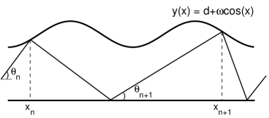
Figure 1: Geometry of the rippled billiard and definition of the variables of map $M$, see Eq. (I).

Figure 2: (Color online) (a) Poincaré map $M$, (b) phase distribution $P(\theta)$, and (c) length distribution $P(\ell)$ for the ripple billiard with $\omega=2\pi/10$ and $d=2\pi$. A single initial condition $x_{0}=\theta_{0}=0.1$ was iterated (a) $10^{4}$ and (b-c) $10^{7}$ times. The red full curve in (c) is Eq. (2).

Among the dynamical information which is lost when applying $\mbox{mod}(2\pi)$ to a map such as $M$, we can mention the length of paths between successive map iterations $\ell\equiv x_{n+1}-x_{n}$, i.e. the length between two successive collisions with the rippled boundary of the billiard. In fact, in Fig. 2(c) we present $P(\ell)$ for the same parameters used to construct Fig. 2(a). From this figure we can clearly see that: (i) even though most of the paths $\ell$ produced by map $M$ are short (i.e. $P(\ell)$ is highly peaked at $P(\ell)=0$), there is a non-negligible probability for very large values of $\ell$ to occur: Notice that the values of $\ell=\pm 1000$ at the edges of Fig. 2(c) mean that a particle has traveled about 160 periods of the rippled billiard between two successive collisions with the rippled boundary and; (ii) $P(\ell)$ decays as a power-law similar to Eq. (1). These two facts are explicit evidences of Lévy flights in the dynamics of map $M$. Thus, the following question becomes pertinent: Can we provide an analytic expression for the shape of $P(\ell)$ given the simple form of map $M$? Fortunately, the answer is positive as we will show it below.

If we consider the dynamics of map $M$ to be in the regime of full chaos then a single trajectory can explore the full available phase space homogeneously, as shown in Fig. 2(a), so $P(\theta)$ is constant and equal to $1/\pi$, as verified in Fig. 2(b). Also, from the second equation in map $M$ we obtain $\theta=\tan^{-1}(2d/\ell)$. Thus, using $P(\ell)=P(\theta)|d\theta/d\ell|$, we can write

$$P(\ell)=\frac{2d}{\pi\left(1+\ell^{2}\right)}\ ,$$ (2)

which is in fact a Lévy-type probability distribution function with $\alpha=1$; compare with Eq. (1). Then, in Fig. 2(c) we plot Eq. (2) (as the red full line) together with the numerically obtained $P(\ell)$ and observe a very good correspondence making clear the existence of Lévy processes, characterized by the power-law decay $\alpha=1$, in the dynamics of the rippled billiard.

In fact, the origin of the Lévy-type probability distribution of Eq. (2) for the lengths $\ell$ in the ripple billiard is the existence of Lévy flights. Since a typical chaotic trajectory fills the available phase space uniformly, see Fig. 2(a), then all angles $\theta\in(0,2\pi)$ are equally probable; however, different angles produce quite different lengths $\ell$. For example, an angle $\theta$ very close to $\pi/2$ corresponds to a very short length $\ell\sim 0$, see Fig. 1. While $\theta$ tending to zero or $\pi$ produce trajectories which are nearly parallel to the $x$-axis that may travel very long distances between successive collisions with the ripple boundary: in such case $\ell\to\infty$. These grazing trajectories are indeed Lévy flights, known to produce heavy-tailed distribution functions M82 ; for the ripple billiard the Lévy flights produce Eq. (2) as derived above. Moreover, grazing trajectories in the ripple billiard have been found to play a prominent role when defining the classical analogs of the quantum structure of eigenstates and local density of states LMI00 .

Equation (2) is already an interesting result on the dynamics of the rippled billiard (and of general chaotic extended billiards with infinite horizon) that deserves additional attention, however our goal here is different. Since now we know that map $M$ produces Lévy flights characterized by $\alpha=1$ we ask ourselves: Can we propose a general 2D non-linear map where $\alpha$ can be included as a parameter? More generally, can we construct the map $M_{\alpha}$ able to produce Lévy flights characterized by $0<\alpha<2$? Indeed, in the following section we elaborate on these questions.

II Derivation of the Lévy Map

We introduce the Lévy Map $M_{\alpha}$ by following the opposite procedure we used above to obtain the distribution function of Eq. (2) from map $M$.

Let us

• consider the 2D map $(\theta_{n+1},x_{n+1})=M_{\alpha}(\theta_{n},x_{n})$ to have the same iteration relation for the angle $\theta$ as map $M$, see Eq. (I),

• assume the map $M_{\alpha}$ to be in a regime of global chaos, such that

  $$P(\theta)=\mbox{const}=\frac{1}{\pi}\ ,$$ (3)

  and

• demand the variable

  $$\ell\equiv x_{n+1}-x_{n}$$ (4)

  from map $M_{\alpha}$ to be characterized by the Lévy-type density distribution function

  $$P(\ell)=\frac{\cal C}{\ell^{1+\alpha}}\ ,$$ (5)

  where $0<\alpha<2$ and $\cal C$ is a normalization constant.

Then,

$$\theta\equiv\int\frac{P(\ell)}{P(\theta)}d\ell=\pi{\cal C}\int\frac{d\ell}{\ell^{1+\alpha}}=-\frac{\pi{\cal C}}{\alpha\ell^{\alpha}}$$

provides $\ell=(-\alpha\theta/\pi{\cal C})^{-1/\alpha}$. Therefore, we define the Lévy Map as

$$M_{\alpha}:\left\{\begin{array}[]{ll}\theta_{n+1}&=\theta_{n}-2\omega\sin(x_{n})\ ,\\ x_{n+1}&=x_{n}+\gamma|\alpha\theta_{n+1}|^{-1/\alpha}\ ,\quad 0<\alpha<2\ ,\end{array}\right.$$

where $\omega$, $\gamma=(\pi{\cal C})^{1/\alpha}$, and $\alpha$ are the map parameters. We have introduced the absolute value in the second equation of $M_{\alpha}$ to avoid fractional powers of negative angles. This, in turn, makes all lengths $\ell$ to be positive.

Notice that for $\alpha=1$ and $\theta_{n+1}\ll 1$, where $\cot(\theta_{n+1})\approx 1/\theta_{n+1}$, we recover map $M$ from $M_{\alpha}$ (with $\gamma=2d$). We also note that $M_{\alpha}$ has a similar form than the maps studied in Refs. OBL10 ; LOS11 ; OL11 ; ODCL13 in the sense that the function $f(\theta_{n+1})$, in the second line of the map $M_{\alpha}$, is inverse proportional to $\theta_{n+1}$ to a non-integer power.

Below we will focus our attention on map $M_{\alpha}$ with the parameter $\alpha$ into the interval $0<\alpha<2$ because our motivation is to construct a map able to produce pseudo-random variables distributed according to $\alpha$-stable distributions. However, the parameter $\alpha$ may also take values outside this interval.

III Onset of global chaos

In general, depending on the values of the parameters $(\omega,\gamma,\alpha)$, the dynamics of the Lévy Map may be integrable, mixed (where the phase space contains periodic islands surrounded by chaotic seas which may be limited by invariant spanning curves), or ergodic. That is, the classical phase space of map $M_{\alpha}$ develops the generic transition to global chaos (not shown here). However, for Eq. (3) to be valid the map dynamics must be ergodic. Therefore, below, by applying Chirikov’s overlapping resonance criteria we shall identify the onset of global chaos as a function of the parameters of the Lévy Map.

Following licht we linearize $M_{\alpha}$ around the period-one fixed points $(x^{*},\theta^{*})$, which are defined through

$$\left\{\begin{array}[]{ll}\theta_{n+1}=\theta_{n}=\theta^{*}\\ x_{n+1}=x_{n}=x^{*}+2\pi m\ ,\quad m=1,2,3,\ldots\\ \end{array}\right.$$

This condition provides

$$x^{*}=0,\pi\qquad\mbox{and}\qquad\theta^{*}=\frac{1}{\alpha}\left(\frac{\gamma}{2\pi m}\right)^{\alpha}\ .$$ (6)

Then, for an angle close to $\theta^{*}$ we can write $\theta_{n}=\theta^{*}+\Delta\theta_{n}$ getting

$$\theta_{n+1} = \theta^{*}+\Delta\theta_{n+1}$$

$$= \theta^{*}+\Delta\theta_{n}-2\omega\sin(x_{n})\ .$$

Thus,

$$\Delta\theta_{n+1}=\Delta\theta_{n}-2\omega\sin(x_{n})\ .$$ (7)

In addition, for $x$ we have

$$x_{n+1} = x_{n}+\gamma\alpha^{-1/\alpha}(\theta^{*}+\Delta\theta_{n+1})^{-1/\alpha}$$ (8)

$$\approx x_{n}+\gamma(\alpha\theta^{*})^{-1/\alpha}[1-(\alpha\theta^{*})^{-1}\Delta\theta_{n+1}]$$

$$= x_{n}+2\pi m[1-(\gamma/2\pi m)^{-\alpha}\Delta\theta_{n+1}]$$

$$= x_{n}-\gamma^{-\alpha}(2\pi m)^{\alpha+1}\Delta\theta_{n+1}\ .$$

Finally, by substituting the new angle

$$\Theta_{n}\equiv-\gamma^{-\alpha}(2\pi m)^{\alpha+1}\Delta\theta_{n}$$

in (7) and (8) we can write the linearized map

$$M_{\mbox{\tiny SM}}:\left\{\begin{array}[]{ll}\Theta_{n+1}=\Theta_{n}+K\sin(x_{n})\\ x_{n+1}=x_{n}+\Theta_{n+1}\\ \end{array}\right.\ ,$$ (9)

where $\Theta$ and $x$, respectively, play the role of action-angle variables in the Standard Map licht ; C69 with

$$K=2(2\pi m)^{\alpha+1}\omega\gamma^{-\alpha}\ ,\quad m=1,2,3,\ldots$$ (10)

being the stochasticity parameter.

Chirikov’s overlapping resonance criteria predicts the transition to global chaos for $K>K_{\mbox{\tiny C}}$, where $K_{\mbox{\tiny C}}\approx 0.971635\ldots$ licht ; C69 ; C79 . Global chaos means that chaotic regions are interconnected over the whole phase space (stability islands may still exist but are sufficiently small that the chaotic sea extends throughout the vast majority of phase space). This criteria for the Lévy Map reads as

$$\omega\stackrel{{\scriptstyle>}}{{\sim}}\frac{\gamma^{\alpha}}{2(2\pi)^{\alpha+1}}=\frac{{\cal C}}{4(2\pi)^{\alpha}}\ .$$ (11)

In fact, to get Eq. (11) from Eq. (10) we have applied the resonance criteria to the period-one fixed point corresponding to $m=1$, see Eq. (6), which is the fixed point having the largest $\theta$ (i.e. it is located highest in phase space) and the one closer to the last invariant spanning curve bounding the diffusion of the variable $\theta$.

Indeed, we have verified that the phase space of $M_{\alpha}$ is ergodic if condition (11) is satisfied (not shown here). Moreover, in Figs. 3(a-d) we plot the phase distribution functions $P(\theta)$ for the Lévy Map with $\omega={\cal C}=1$ corresponding to $\alpha=1/4$, 1/2, 1, and 3/2. From these figures, it is clear that $P(\theta)$ is certainly a constant distribution. In particular, note that with $\omega={\cal C}=1$ condition (11) is satisfied for any $\alpha$, so we shall use this set of parameter values in all figures below.

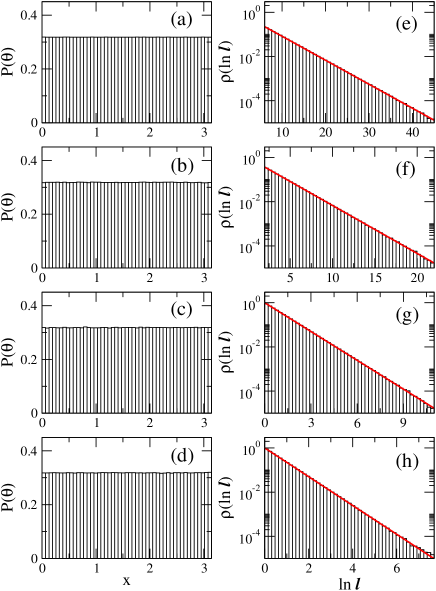
Figure 3: (Color online) (a-d) Phase distributions $P(\theta)$ and (e-h) length distributions $\rho(\ln\ell)$ for the Lévy Map $M_{\alpha}$ with $\omega={\cal C}=1$. (a,e) $\alpha=1/4$, (b,f) $\alpha=1/2$, (c,g) $\alpha=1$, and (d,h) $\alpha=3/2$. To construct each histogram a single initial condition $x_{0}=\theta_{0}=0.1$ was iterated $10^{7}$ times. The red full curve in (e-h) is $\rho(\ln\ell)=\ell^{-\alpha}$.

Now we would like to verify that once $P(\theta)=1/\pi$, $M_{\alpha}$ must produce lengths $\{\ell\}$ distributed according to Eq. (5). However, we noticed that for $\alpha<1$ the Lévy Map produces huge values of $\ell$. To show this, in Fig. 4 we plot the typical value of $\ell$,

$$\ell_{\mbox{\tiny typ}}=\exp\left\langle\ln\ell\right\rangle\ ,$$ (12)

as a function of $\alpha$; where we can observe that for $\alpha=1/4$ the typical $\ell$ is larger than $10^{5}$ (in fact, from the data we used to construct the $P(\theta)$ of Fig. 3(a) we obtained several lengths $\ell$ of the order of $10^{30}$!). Thus, it is not practical to construct $P(\ell)$ to test the validity of Eq. (5) itself. Instead, we make the change of variable $\ell\to\ln\ell$ which leads to

$$\rho(\ln\ell)=\ell P(\ell)=\frac{{\cal C}}{\ell^{\alpha}}\ .$$

Then in Figs. 3(e-h) we show length distribution functions $\rho(\ln\ell)$ for the Lévy Map with $\alpha=1/4$, 1/2, 1, and 3/2 (histograms). As clearly seen, the agreement between the histograms and $\rho(\ln\ell)=\ell^{-\alpha}$ (shown as red thick lines) is indeed excellent.

It is relevant to stress that since the phase space of the Lévy Map is ergodic when condition (11) is satisfied, the sequences $\{\ell\}$ can then be considered as Lévy-distributed pseudo-random numbers. In fact, in the next Section we will show through a specific application that the lengths $\ell$ can be used in practice as random numbers.

Figure 4: Typical value of $\ell$, $\ell_{\mbox{\tiny typ}}=\exp\left\langle\ln\ell\right\rangle$, for the Lévy Map $M_{\alpha}$ as a function of $\alpha$. $\omega={\cal C}=1$ were used. The average was performed over $10^{7}$ values of $\ell$ obtained by iterating $M_{\alpha}$ from the single initial condition $x_{0}=\theta_{0}=0.1$.

IV The Lévy Map as a Lévy-distributed pseudo-random number generator

There is a good deal of work devoted to the use of non-linear maps as pseudo-random number generators, see some examples in Refs. pseudo1 ; pseudo2 ; pseudo3 ; pseudo4 ; pseudo5 ; pseudo6 . Therefore, in a similar way, we would like to use the Lévy Map to generate pseudo-random numbers particularly distributed according to the Lévy-type probability distribution function of Eq. (5). However, instead of analyzing the randomness of the sequences $\{\ell\}$ produced by $M_{\alpha}$, here we will show that these numbers can be successfully used already in a specific application: We shall compute transmission through one-dimensional (1D) disordered wires.

Recently, the electron transport through 1D quantum wires with Lévy-type disorder was studied in Refs. FG10 ; FG12 . There, it was found that the average (over different disorder realizations) of the logarithm of the dimensionless conductance $G$ behaves as

$$\left\langle-\ln G\right\rangle\propto\left\{\begin{array}[]{ll}L^{\alpha}&\mbox{for}\quad 0<\alpha<1\\ L&\mbox{for}\quad 1\leq\alpha<2\end{array}\right.\ .$$ (15)

where $L$ is a length that depends on the wire model. For example, for a wire represented as a sequence of potential barriers with random lengths, $L=\sum_{n}\nu_{n}$ FG10 ; where $\nu_{n}$ is the length of the $n$th barrier in the wave propagation direction. While for a wire represented by the 1D Anderson model with off-diagonal disorder, $L=\sum_{n}\nu_{n,n+1}$ FG12 ; where $\nu_{n,n+1}$ is the hopping integral between the sites $n$ and $n+1$.

Here, we use the 1D Anderson model with off-diagonal disorder to represent 1D quantum wires (see details in the Appendix) where the hopping integrals $\nu_{n,n+1}$ are, in fact, the pseudo-random lengths $\ell$ generated by our Lévy Map. Then, in Fig. 5 we plot $\left\langle-\ln G\right\rangle$ as a function of $L$ for the 1D Anderson Model with Lévy-type disorder characterized by $\alpha=1/4$, 1/2, 1, and 3/2. We have computed the dimensionless conductance by the use of the effective Hamiltonian approach (see details in the Appendix). In Fig. 5 we are using $\ell_{\mbox{\tiny typ}}$ to normalize $L$ to be able to show curves corresponding to different values of $\alpha$ into the same figure panel. Also, in Fig. 5 we are including fittings of the curves $\left\langle-\ln G\right\rangle$ vs. $L$ with Eq. (15), see red dashed lines, which certainly show the anomalous conductance behavior predicted in Refs. FG10 ; FG12 . Therefore, validating in this way the use of the Lévy Map as a pseudo-random number generator.

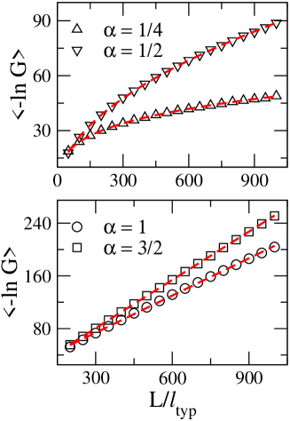
Figure 5: The average $\left\langle-\ln G\right\rangle$ as a function of $L/\ell_{\mbox{\tiny typ}}$ for the 1D Anderson Model with off-diagonal Lévy-type disorder characterized by $\alpha$. We used an incoming wave with energy $E=0.1$. The dashed lines are fittings of the data with Eq. (15). Each symbol was calculated using $10^{5}$ wire realizations. Each wire realization is constructed from a single sequence of lengths $\{\ell\}$ generated by map $M_{\alpha}$ having random initial conditions uniformly distributed in the intervals $-\pi<x_{0}<\pi$ and $0<\theta_{0}<2\pi$.

V Conclusions

In this paper we have introduced the so-called Lévy Map: A two-dimensional nonlinear map characterized by tunable Lévy flights. Indeed it is described by a 2D nonlinear and area preserving map with a control parameter driving two important transitions: (i) integrability ($\omega=0$) to non-integrability ($\omega\neq 0$) and; (ii) local chaos with $\omega<C/4(2\pi)^{\alpha}$ to globally chaotic dynamics with $\omega>C/4(2\pi)^{\alpha}$. We have applied Chirikov’s overlapping resonance criteria to identify the onset of global chaos as a function of the parameters of the map therefore reaching to condition (ii) as described on the line above. In this way we stated the requirements under which the Lévy Map could be used as a Lévy pseudo-random number generator and confirmed its effectiveness by computing scattering properties of disordered wires.

VI Appendix

In Sect. IV we have considered 1D tight-binding chains of size $N$ described by the Hamiltonian

$$H_{mn}=h_{n}\delta_{mn}+\nu_{n,n+1}\delta_{n,n+1}+\nu_{n,n-1}\delta_{n,n-1}\ ,$$ (16)

where $h_{n}$ are on-site potentials that we set to zero and $\nu_{n,n+1}=\nu_{n+1,n}$ are hopping amplitudes connecting nearest sites. Here, $m,n=1\ldots N$.

We open the 1D chains by attaching two single-mode semi-infinite leads to the opposite sites on the 1D samples. Each lead is described by the 1D semi-infinite tight-binding Hamiltonian

$$H_{\mbox{\tiny lead}}=\sum^{-\infty}_{n=1}(|n\rangle\langle n+1|+|n+1\rangle\langle n|)\ .$$

Then, following the effective Hamiltonian approach, the scattering matrix ($S$-matrix) has the form MW69

$$S=\left(\begin{array}[]{cc}r&t^{\prime}\\ t&r^{\prime}\end{array}\right)={\bf 1}-2\pi\mbox{i}\,{\cal W}^{\,T}\frac{1}{E-{\cal H}_{\rm eff}}{\cal W}\ .$$ (17)

where $t$, $t^{\prime}$, $r$, and $r^{\prime}$ are transmission and reflection amplitudes; ${\bf 1}$ is the $2\times 2$ unit matrix, $k=\arccos(E/2)$ is the wave vector supported in the leads, and ${\cal H}_{\rm eff}$ is an effective energy-dependent non-hermitian Hamiltonian given by

$${\cal H}_{\rm eff}=H+\pi\cot(k){\cal W}{\cal W}^{\,T}-\mbox{i}\pi{\cal W}{\cal W}^{\,T}\ .$$ (18)

Above, ${\cal W}$ is a $L\times 2$ matrix with elements ${\cal W}_{i,j}=[\sin(k)/\pi]^{1/2}(\delta_{1,1}+\delta_{L,2})$.

Finally within a scattering approach to electronic transport, once the scattering matrix is known we compute the dimensionless conductance as Landauer

$$G=|S_{12}|^{2}\ .$$ (19)

Acknowledgments. J.A.M.-B is grateful to FAPESP (2013/14655-9) Brazilian agency; partial support form VIEP-BUAP grant MEBJ-EXC14-I and Fondo Institucional PIFCA 2013 (BUAP-CA-169) is also acknowledged. J.A.M.-B also thanks the warm hospitality at Departamento de Física at UNESP – Rio Claro, where this work was mostly developed. J.A.O thanks PROPe/FUNDUNESP/UNESP. E.D.L. thanks to FAPESP (2012/23688-5), CNPq, and CAPES, Brazilian agencies.

References

- (1) V. V. Uchaikin and V. M. Zolotarev, Chance and Stability. Stable Distributions and their Applications (VSP, Utrecht, 1999).
- (2) G. M. Viswanathana, E. P. Raposo, and M. G. E. da Luz, Physics of Life Reviews 5, 133 (2008).
- (3) D. Brockmann, L. Hufnagel, and T. Geisel, Nature 439, 462 (2006).
- (4) O. Sotolongo-Costa, J. C. Antoranz, A. Posadas, F. Vidal, and A. Vazquez, Geophysical Research Letters 27, 1965 (2000).
- (5) T. Botari, S. G. Alves, and E. D. Leonel, Phys. Rev. E 83, 037101 (2011).
- (6) P. Barthelemy, J. Bertolotti, and D. S. Wiersma, Nature 453, 495 (2008).
- (7) A. Clauset, C. R. Shalizi, and M. E. J. Newman, SIAM Review 51, 661 (2009).
- (8) L. E. Reichl, The Transition to Chaos (Springer-Verlag, New York, 2004).
- (9) A. J. Lichtenberg and M. A. Lieberman, Regular and Chaotic Dynamics (Springer-Verlag, New York, 1992).
- (10) G. A. Luna-Acosta, K. Na, L. E. Reichl, and A. Krokhin, Phys. Rev. E 53, 3271 (1996); A. J. Martínez-Mendoza, J. A. Méndez-Bermúdez, G. A. Luna-Acosta, and N. Atenco-Analco, Rev. Mex. Fis. S 58, 6 (2012).
- (11) E. D. Leonel, Phys. Rev. Lett. 98, 114102 (2007); E. D. Leonel, D. R. da Costa, and C. P. Dettmann, Phys. Lett. A 376, 421 (2012).
- (12) B. B. Mandelbrot, The Fractal Geometry of Nature (Freeman, New York, 1982).
- (13) G. A. Luna-Acosta, J. A. Méndez-Bermúdez, and F. M. Izrailev, Phys. Lett. A 274, 192 (2000); Phys. Rev. E 64, 036206 (2001).
- (14) J. A. de Oliveira, R. A. Bizão, and E. D. Leonel, Phys. Rev. E 81, 046212 (2010).
- (15) E. D. Leonel, J. A. de Oliveira, and F. Saif, J. Phys. A: Math. Theor. 44, 302001 (2011).
- (16) J. A. de Oliveira and E. D. Leonel, Physica A 390, 3727 (2011).
- (17) J. A. de Oliveira, C. P. Dettmann, D. R. da Costa, and E. D. Leonel, Phys. Rev. E 87, 062904 (2013).
- (18) B. V. Chirikov, Preprint 267, Institute of Nuclear Physics, Novosibirsk (1969) [Engl. Trans., CERN Trans. 71-40 (1971)].
- (19) B. V. Chirikov, Phys. Rep. 52, 263 (1979).
- (20) T.-Y. Li and J. A. Jorke, Nonlinear Anal. Theory Methods Appl. 2, 473 (1978).
- (21) S. C. Phatak and S. S. Rao, Phys. Rev. E 51, 3670 (1995).
- (22) J. A. Gonzalez, L. I. Reyes, J. J. Suarez, L. E. Guerrero, and G. Gutierrez, Phys. Lett. A 295, 25 (2002); Physica A 316, 259 (2002); Physica D 178, 26 (2003).
- (23) S. Sanchez, R. Criado, and C. Vega, Mathematical and Computing Modelling 42, 809 (2005).
- (24) K. Wang, W. Pei, H. Xia, and Y. Cheung, Phys. Lett. A 372, 4388 (2008).
- (25) A. Kanso and N. Smaoui, Chaos Sol. Frac. 40, 2557 (2009).
- (26) F. Falceto and V. A. Gopar, Europhys. Lett. 92, 57014 (2010).
- (27) I. Amanatidis, I. Kleftogiannis, F. Falceto, and V. A. Gopar, Phys. Rev. B 85, 235450 (2012).
- (28) C. Mahaux and H. A Weidenmüller, Shell Model Approach in Nuclear Reactions, (North-Holland, Amsterdam,1969); J. J. M. Verbaarschot, H. A. Weidenmüller, and M. R. Zirnbauer, Phys. Rep. 129, 367 (1985); I. Rotter, Rep. Prog. Phys. 54, 635 (1991).
- (29) R. Landauer, IBM J. Res. Dev. 1, 223 (1957); 32, 336 (1988); M. Buttiker, Phys. Rev. Lett. 57, 1761 (1986); IBM J. Res. Dev. 32, 317 (1988).