Active Viscoelastic Matter: from Bacterial Drag Reduction to Turbulent Solids

Abstract

A paradigm for internally driven matter is the active nematic liquid crystal, whereby the equations of a conventional nematic are supplemented by a minimal active stress that violates time-reversal symmetry. In practice, active fluids may have not only liquid-crystalline but also viscoelastic polymer degrees of freedom. Here we explore the resulting interplay by coupling an active nematic to a minimal model of polymer rheology. We find that adding polymer can greatly increase the complexity of spontaneous flow, but can also have calming effects, thereby increasing the net throughput of spontaneous flow along a pipe (a ‘drag-reduction’ effect). Remarkably, active turbulence can also arise after switching on activity in a sufficiently soft elastomeric solid.

Active materials include bacterial swarms in a fluid, the cytoskeleton of living cells, and ‘cell extracts’ containing just filaments, molecular motors, and a fuel supply RMP ; Cisneros ; Actomyosin ; Dogic . Such materials are interesting because of their direct biophysical significance, and as representatives of a wider class of systems in which deviations from thermal equilibrium are not created by initial or boundary conditions (a temperature quench, or motion of walls in a shear cell) but arise microscopically in the dynamics of each particle. By continually converting chemical energy into motion, active matter violates time-reversal symmetry, suspending the normal rules of thermal equilibrium dynamics (until the fuel runs out), causing strongly non-equilibrium features such as spontaneous flow. This flow may remain steady and laminar at the scale of the system; may show limit cycles at that scale or below; or may show spatiotemporal chaos. Since it resembles the inertial turbulence of a passive Newtonian fluid, the latter outcome is commonly called ‘bacterial’ (or ‘active’) turbulence Cisneros ; MarenduPRE ; YeomansPNAS ; CristinaDefect ; CristinaDefectPreprint ; Thampi . The mechanism is quite distinct, however, stemming from a balance between active stress and orientational relaxation, rather than between inertia and viscosity as in conventional turbulence.

The phenomenology of activity-driven spontaneous flow can be understood, to a remarkable extent, using conceptually simple continuum models RMP ; SRreview ; Simha ; Joanny . These start from the hydrodynamic equations of a passive fluid of rod-like objects with either polar Joanny or nematic Simha local order, the latter characterized by a tensor order parameter ${\bf Q}({\bf r})$ Simha . To the passive equations for such a liquid crystal (LC) BerisEdwards are then added leading-order violations of time-reversal symmetry; after renormalization of passive parameters and allowing for fluid incompressibility, what remains is a bulk stress $\mathbf{\Sigma}_{A}=-\zeta{\bf Q}$ where $\zeta$, an activity parameter, is positive for extensile systems, negative for contractile. In extensile materials each rodlike particle pulls fluid inwards equatorially and emits it symmetrically from the poles, with the reverse for the contractile case. Even without accurate knowledge of $\zeta$, this approach makes robust predictions. For example, extensile and contractile systems become separately unstable toward spontaneous flow states at critical activity levels that are system-size dependent, and vanish for bulk samples. Numerical solution of the active nematic equations MarenduPRE ; CristinaDefect ; CristinaDefectPreprint ; Thampi show spontaneous flows resembling experiments on bacterial swarms Cisneros and on microtubule-based cell extracts Dogic . Both of these are extensile nematics, and we restrict ourselves to this case below AsterNote .

Active nematogenic fluids are often referred to as ‘active gels’ Joanny ; MarenduPRE . But although all LCs are somewhat viscoelastic (due to slow defect motion) these models assume fast local relaxations and mostly do not address gels in a conventional sense Callan . Certainly they do not capture the diversity of viscoelastic behavior that one expects in sub-cellular active matter containing long-chain flexible polymers, or other cytoplasmic components, with long (possibly divergent) intrinsic relaxation times. These slow relaxations should couple to the orientational order, strongly modifying the effects of activity. Polymers could also play a strong role in modifying diffusion Contrary and active flows at supra-cellular level: they are present in mucus, saliva, and other viscoelastic fluids in which swarms of motile bacteria reside. Notably, many bacteria excrete their own polymers Exo-polymer , suggesting an advantage in controlling the viscoelasticity of their surroundings.

In this Letter, therefore, we present a model that addresses the interplay between active LC and polymers Callan . We sketch its derivation (which requires care) and give examples of its rich dynamics (which will be explored further in EwanLong ). Highlights include: an exotic form of ‘drag reduction’ by polymers for active (non-inertial) turbulence; spontaneous flows with slow polymer-driven oscillations; and transient active turbulence within a material that is ultimately a solid.

Equations of Motion: The symmetric and antisymmetric parts of the centre-of-mass velocity-gradient tensor $\left(\nabla\mathbf{v}\right)_{ij}\equiv\partial_{i}v_{j}$ are denoted $\mathbf{D}$ and $\mathbf{\Omega}$ FootIndex . For other tensors the symmetric, antisymmetric, and traceless parts carry superscripts S,A and T. Conformation tensors for the polymer and LC are denoted $\mathbf{C}$ and $\mathbf{Q}$, where $\mathbf{Q}$ is traceless. The polymeric tensor is $\mathbf{C}=\langle{\bf rr}\rangle$, where ${\bf r}$ is the end-to-end vector of a chain (or subchain, depending on the level of description). We introduce a free energy density $f=f_{Q}(\mathbf{Q},\nabla\mathbf{Q})+f_{C}(\mathbf{C})+f_{QC}(\mathbf{Q},\mathbf{C})$ where $f_{Q}$ and $f_{C}$ are standard forms for active nematics BerisEdwards and dumb-bell polymers Milner respectively, as detailed in SI . The lowest order passive coupling is

$$f_{QC}=\kappa\textrm{Tr}\left[\mathbf{C}-\mathbf{I}\right]\textrm{Tr}\left[\mathbf{Q}^{2}\right]+2\chi\textrm{Tr}\left[\mathbf{C}\mathbf{Q}\right].$$ (1)

Both terms vanish for undeformed polymers ($\mathbf{C}=\mathbf{I}$).

From the free energy $F=\int fdV$ we next derive the nematic molecular field $\mathbf{H}\equiv-(\delta F/\delta\mathbf{Q})^{\rm ST}$ as

$$\mathbf{H} =-G_{Q}\left[\left(1-\frac{\gamma}{3}\right)\mathbf{Q}-\gamma\mathbf{Q}^{2}+\gamma\mathbf{Q}^{3}\right]-G_{Q}\gamma\frac{\mathbf{I}}{3}\textrm{Tr}\left[\mathbf{Q}^{2}\right]$$ (2)

$$+K\nabla^{2}\mathbf{Q}-2\kappa\textrm{Tr}\left[\mathbf{C}-\mathbf{I}\right]\mathbf{Q}-2\chi\mathbf{C}^{\rm T}.$$

Here $G_{Q}$ is a bulk free energy density scale set by $f_{Q}$; $K$ is the nematic elastic constant; $\gamma$ a control parameter for the nematic transition; and $G_{C}$ the polymer elastic modulus. (See details in SI .) The corresponding molecular field for polymer conformations is simpler: $\mathbf{B}\equiv-(\delta F/\delta\mathbf{C})=-G_{C}(\mathbf{I}-\mathbf{C}^{-1})/2-\kappa\mathbf{I}\textrm{Tr}\left[\mathbf{Q}^{2}\right]-2\chi\mathbf{Q}$.

The most general equations of motion then involve at least four separate 4th-rank tensors describing how $\mathbf{Q}$ and $\mathbf{C}$ respond to these molecular fields, and to imposed velocity gradients. For simplicity we choose the response tensors of the Beris-Edwards LC theory and the Johnson-Segalman (JS) polymer model respectively BerisEdwards . We then allow for conformational diffusion in the polymer sector StressDiffusion which adds a gradient term in $\mathbf{C}$ of kinetic origin SI . The result is a minimally coupled model of the passive $\mathbf{C}+\mathbf{Q}$ dynamics that reduces to well-established models when either order parameter is suppressed.

To the coupled passive model we finally add a minimal set of active terms Simha . In principle one can add all terms that violate time reversal symmetry arising at zeroth order in gradients and first order in either $\mathbf{Q}$ or $\mathbf{C}-\mathbf{I}$; these are given in SI . Here we suppose for simplicity that the polymers are not themselves active, and respond to nematic activity only through fluid advection. This captures the effect of adding polymer to (say) a cell extract; alternatively this could describe the collective dynamics of bacterial suspensions in mucus. (In contrast, one could build a system of polymers directly from active elements RjoyPol .) There remain two active terms linear in $\mathbf{Q}$; one can be absorbed into $f_{Q}$, and the other is the familiar active deviatoric stress $\mathbf{\Sigma}_{A}=-\zeta\mathbf{Q}$ Simha .

The resulting equations of motion for $\mathbf{Q}$ and $\mathbf{C}$ are:

$$\left(\partial_{t}+\mathbf{v}.\nabla\right)\mathbf{Q}=\mathbf{Q}\mathbf{\Omega}-\mathbf{\Omega}\mathbf{Q}+\frac{2\xi}{3}\mathbf{D}+2\xi\left[\mathbf{Q}\mathbf{D}\right]^{\rm ST}$$

$$-2\xi\mathbf{Q}\textrm{Tr}\left[\mathbf{Q}\mathbf{D}\right]+\tau_{Q}^{-1}\mathbf{H}/G_{Q},$$ (3)

$$\left(\partial_{t}+\mathbf{v}.\nabla\right)\mathbf{C}=\mathbf{C}\mathbf{\Omega}-\mathbf{\Omega}\mathbf{C}+2a\left[\mathbf{C}\mathbf{D}\right]^{\rm S}$$

$$+\tau_{C}^{-1}(2\left[\mathbf{B}\mathbf{C}\right]^{\rm S}/G_{C}+\ell^{2}_{C}\nabla^{2}\mathbf{C}).$$ (4)

Here $\xi$ is the flow-alignment parameter of the nematic Stark and $a$ is the slip parameter of the JS model. Each controls the relative tendency of molecules to align with streamlines and rotate with local vorticity. Parameters $\tau_{Q},\tau_{C}$ are intrinsic relaxation times for nematic and polymer, while $\ell_{C}$ governs diffusion in the JS sector StressDiffusion .

The incompressible fluid velocity $\mathbf{v}$ obeys the Navier Stokes equation $\rho\left(\partial_{t}+v_{\beta}\partial_{\beta}\right)v_{\alpha}=\partial_{\beta}\left(\Sigma_{\alpha\beta}\right)$ whose stress $\mathbf{\Sigma}=-P\mathbf{I}+2\eta\mathbf{D}+\mathbf{\Sigma}_{A}+\mathbf{\Sigma}_{Q}+\mathbf{\Sigma}_{C}$ combines an isotropic pressure $P$, a contribution from a Newtonian solvent of viscosity $\eta$, and active stress $\mathbf{\Sigma}_{A}$ with two reactive stresses Colon

$$\mathbf{\Sigma}_{Q} = -K(\nabla\mathbf{Q}):(\nabla\mathbf{Q})+2\left[\mathbf{Q}\mathbf{H}\right]^{\rm A}$$ (5)

$$- \frac{2\xi}{3}\mathbf{H}-2\xi\left[\mathbf{Q}\mathbf{H}\right]^{\rm ST}+2\xi\mathbf{Q}\textrm{Tr}\left[\mathbf{Q}\mathbf{H}\right],$$

$$\mathbf{\Sigma}_{C} = -2a\left[\mathbf{C}\mathbf{B}\right]^{\rm S}+2\left[\mathbf{C}\mathbf{B}\right]^{\rm A}.$$ (6)

Crucially, $\xi$ and $a$ must appear as shown in the reactive stresses to recover a correct passive limit BerisEdwards . In the pure JS case, but not in general, one can absorb the factor $a$ in (6) into $G_{C}$, restoring consistency to the classical JS model, which sets $\mathbf{\Sigma}_{C}=-2\mathbf{B}\mathbf{C}$ for all $a$ BerisEdwards ; Olmsted . A less careful marriage of JS with active nematic theory would thus have set $a=1$ in (6) but not (4), violating thermodynamic principles Ottinger and giving incorrect physics.

Parameter Choices: We choose $\xi$ and $a$ within the flow-aligning and outwith the shear-banding ranges of their respective models, to avoid tumbling and banding instabilities of the passive model in flow. We neglect inertia ($\rho=0$), and choose units where $G_{Q}=\tau_{Q}=L_{y}=1$, with $L_{y}$ the width of the sample, a 2D simulation box of $L_{x}\times L_{y}=4\times 1$. We choose periodic boundary conditions in $x$, with no-slip (of $\mathbf{v}$) and no-gradient (of $\mathbf{Q}$ or $\mathbf{C}$) at the sample walls ($y=0,L_{y}$). Default values for numerics are $\xi=0.7,\eta=0.567$ and $\gamma=3$ (directly comparable with Ref. MarenduPRE for the polymer-free case); we set $a=1$. We vary $\tau_{C}$ over several decades $10^{-2}\leq\tau_{C}\leq 10^{6}$ at fixed polymer viscosity $\eta_{C}\equiv\tau_{C}G_{C}=1$, allowing fast or slow relaxation while retaining comparability of $\mathbf{\Sigma}_{Q,C}$. We define $\ell_{Q}=(K/G_{Q})^{1/2}$, the Frank length for nematic distortions, and vary this in the range $0.002\leq\ell_{Q}/L_{y}\leq 0.025$ (comparable to other studies MarenduPRE ; YeomansPNAS ), and then set $\ell_{C}^{2}/\tau_{C}=\ell_{Q}^{2}/\tau_{Q}$ to equate the diffusivities of ${\bf Q}$ and ${\bf C}$. Using careful numerics we are able to address several decades of activity level $10^{-4}\leq\zeta\leq 6$. Finally, most of our work addresses the simplest case where the coupling of $\mathbf{Q}$ and $\mathbf{C}$ is purely kinematic: i.e., $\kappa=\chi=0$. In this limit, interaction between polymer and $\mathbf{Q}$ is indirect, mediated only via the background fluid velocity $\mathbf{v}$. However we also present some results for nonzero $\chi$, as arises in passive nematic elastomers Warner .

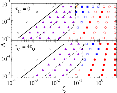
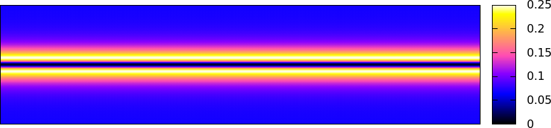
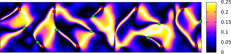
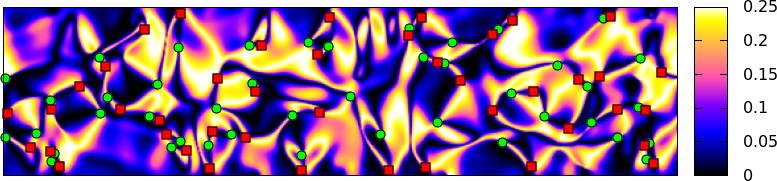
Figure 1: State diagrams without (upper) and with (lower) polymer of relaxation time $\tau_{C}=4\tau_{Q}$. Initial condition: director $\mathbf{n}$ (i.e., major axis of $\mathbf{Q}$) uniformly along $y$. Symbols: $\times$: quiescent; squares: oscillatory; triangles: steady banded flow (cf MarenduPRE ; FieldingPRL ), circles: unsteady/chaotic. Filled symbols denote states with a significant net throughput (along the periodic direction $x$) . Lines show (solid) the 1D instability (bending mode) of the specified initial condition; (dotted) that of the splay mode for initial condition with $\mathbf{Q}$ along $x$, and (dashed) the observed crossover line $\zeta_{c}^{\rm bend2D}$ beyond which the phase diagram becomes independent of which of these initial states was chosen. The bottom three panels show states, all with net throughput, from the $\tau_{C}=4$ phase diagram above: banded ($\zeta=0.023$, $\Delta=10^{-5}$), oscillatory ($\zeta=0.741$, $\Delta=1.6\times 10^{-4}$) and chaotic ($\zeta=1.75$, $\Delta=8\times 10^{-5}$); colour scale indicates $\left(n_{x}n_{y}\right)^{2}$. Defects of topological charge $\pm 1/2$ are identified by green dots (+) and red squares (-).

Results: First, with kinematic coupling only, we ask whether addition of polymer can suppress the intrinsic instability of active nematics towards bulk flow. Generalizing previous results Joanny ; EdwardsYeomans ; MarenduPRE ; Giomi , a linear stability analysis (detailed in Ref. SI ) allowing 1D perturbations of wavevector $\mathbf{k}$ about the quiescent nematic base state gives a critical activity level (for $\gamma=3$)

$$\zeta_{c}=\frac{12k^{2}\ell_{Q}^{2}}{\Lambda\tau_{Q}}\left(\eta+\frac{\Lambda^{2}G_{Q}\tau_{Q}}{72}+\frac{a^{2}\eta_{C}}{1+k^{2}\ell^{2}_{C}}\right),$$ (7)

where $\Lambda=5\xi\pm 3$ for $\mathbf{k}$ perpendicular $(-)$ or parallel $(+)$ to the major axis of $\mathbf{Q}$. Thus $\zeta_{c}$ always vanishes in bulk (as $k\to 0$), while the final term shows a stabilizing effect of polymer in finite systems. This effect is viscous and not viscoelastic in character, since at threshold, the time-scale for growth diverges, with $\tau_{C}$ then infinitely fast in comparison. This analysis, which we have confirmed numerically (Fig. 1), contrasts with Ref.Contrary which reports polymer-induced bulk stabilization for a related but distinct active model (with no inherent nematic tendency).

Fig. 1 shows phase diagrams on the $\zeta,\Delta$ plane, where $\Delta\equiv(\ell_{Q}/L_{y})^{2}$ represents the stabilizing effect of small sample sizes. Varying $\tau_{C}$ at fixed $\eta_{C}=1$ reveals a very interesting effect of strictly viscoelastic origin. Among states showing active turbulence, adding polymer significantly extends the parameter range in which macroscopic symmetry is broken (filled symbols in Fig. 1), as judged by a criterion (see SI ) of significant net throughput of fluid along the (periodic) $x$ direction. Thus adding polymer to (say) a fluid showing bacterial turbulence should effectively ‘reduce drag’ by enhancing throughput at fixed (active) stress – as it does for pressure-driven turbulent pipe flow in a passive fluid DragReduct . The polymer calms the short scale structure of the active flow, decreasing the nematic defect density and increasing the flow correlation length towards the system size, thereby favoring restoration of a more organized flow state.

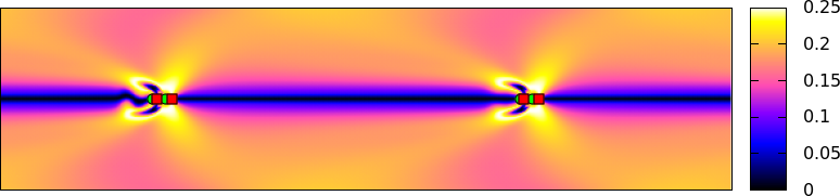
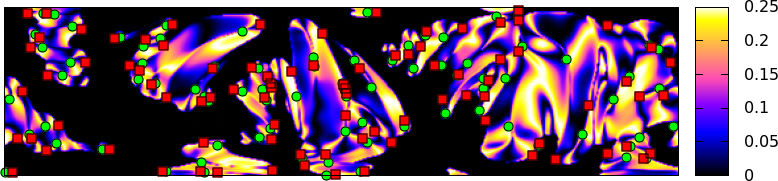
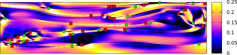
Figure 2: Three spontaneous flow states seen with added polymer, all with $\tau_{C}=10$. Upper frame: a pair of defects traveling along the interface of a shear-banded state ($\zeta=3.2$, $\Delta=10^{-4},\chi=0.002$). Middle frame: coexistence of ‘bubbling’ active domains and regions where the director is out of plane (black) ($\zeta=6$, $\Delta=10^{-4}$, $\chi=0.004$). Lower frame: an exotic oscillatory state which coherently ‘shuffles’ left and right on timescale $\tau_{C}$ ($\zeta=6$, $\Delta=10^{-4}$, $\chi=0.002$). Colour scale indicates $\left(n_{x}n_{y}\right)^{2}$.

This calming effect of polymer on active flow can be reversed by adding direct coupling alongside the kinematic one. Of the two couplings in $f_{QC}$, only the $\chi$ term is sensitive to the relative orientation of tensors $\mathbf{C}$ and $\mathbf{Q}$; the disruptive case is $\chi>0$ so that these tensors want to be misaligned. Fig. 2 shows three novel flow states; for movies see SI2 . Among these are a shear banded state with interfacial defects (related to those seen in CristinaDefectPreprint ; Thampi2 ); coexistence of ‘bubbling’ active domains and regions with director along the vorticity axis; and states showing periodic modulation of a complex flow pattern on a long time scale set by $\tau_{C}$, confirming a direct role for polymer viscoelasticity in creating these new states.

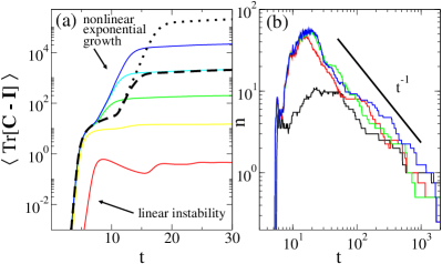
Figure 3: (a) A scalar measure of polymer stress, $\langle\textrm{Tr}\left[\mathbf{C-I}\right]\rangle$, against time for $\tau_{C}=10^{0}$ (bottom, red) $\to 10^{4}$ (top, blue) at fixed $\eta_{C}=1$. Data for $\tau_{C}$ infinite, $G_{C}=10^{-3}$ (bold dashed), $10^{-5}$ (bold dotted) are also shown. (b) Areal defect density $n$ against time for infinite $\tau_{C}$, with $G_{C}=10^{-1}$ (black, bottom) $\to 10^{-7}$ (blue, top); steps arise because $n$ is discrete. In both panels, $\zeta=3.2$, $\Delta=8\times 10^{-5}$.

New and unexpected physics can also arise when this long polymeric time scale becomes effectively infinite, as would describe an active nematic (such as an actomyosin cell extract) within a background of lightly cross-linked elastomer. We address this limit in two ways: first by increasing $\tau_{C}$ (holding $\eta_{C}=1$), then with $\tau_{C}$ infinite at small finite $G_{C}$ (giving infinite $\eta_{C}$). The passive limit of this system is a nematic elastomer Warner ; a full theoretical treatment of the active counterpart will be presented elsewhere ElastomerStability . One might expect all of the flow instabilities reported above to be completely absent in what is, after all, a solid material. But this expectation turns out to be misleading. Since $G_{C}\ll G_{Q}$, the sample can strongly deform before its small elastic modulus has appreciable effects PolyGlass . Accordingly the system should initially show a spontaneous flow instability as though no polymer were present, possibly allowing complex LC textures to form, which then must respond to a growing polymer stress. Numerically (setting $\chi=0$ for simplicity) we indeed find the onset of spontaneous flow. For $\tau_{C}\lesssim\tau_{Q}=1$ the dynamics is essentially the same as without polymer, and the exponential growth of a shear banding instability is tracked by the polymer stress. We have checked that these observations are stable for small, negative values of $\chi$.

Strikingly, for $\tau_{C}\gtrsim\tau_{Q}$, the first phase of exponential growth is followed by a second one (Fig. 3a), arising because the active turbulent state – like its passive inertial counterpart – contains regions of extensional flow where polymers stretch strongly in time. Although for small $G_{C}$ large local strains are needed to arrest the spontaneous flow, the time needed to achieve these grows only logarithmically as $G_{C}\to 0$. For $\tau_{C}\gg\tau_{Q}$, rather soon after its initial formation, the turbulent state indeed arrests into a complex but almost frozen defect pattern. Thereafter the defect density decays slowly, roughly as $t^{-1}$ (see Fig. 3b for $\tau_{C}\to\infty$ case), which is the classical result for passive nematic coarsening Bray . This process is slow enough that the strain pattern created by the arrested active turbulence might easily be mistaken for a final steady state. Our arrest mechanism, where strong polymer stretching in extensional flow regions creates strong stresses in opposition, may relate closely to the drag reduction effects reported above.

Conclusion: To address active viscoelastic matter, we have created a continuum model combining the theory of active nematics with the well-established Johnson-Segalman (JS) model of polymers. In the passive limit, our model is thermodynamically admissible by design – a nontrivial achievement since the JS model itself is admissible only by accident. Our model shows that polymers can shift, but not destroy, the generic instability to spontaneous flow shown by active nematics above a critical activity (which still vanishes for large systems). They can also have a strong ‘bacterial drag reduction’ effect, promoting finite throughput in states of active turbulence.

An antagonistic coupling between polymer and nematic orientations produces instead new and complex spontaneous flows, some with oscillation periods set by the polymer relaxation time. Finally, the elastomeric limit of our model reveals, strikingly, that classifying a material as a solid does not a priori preclude its showing turbulent behavior. Though implausible for inertial turbulence, in the active case this outcome, which arises when $G_{C}/G_{Q}\lesssim 0.1$, looks experimentally feasible for subcellular active matter (though probably not swarms of bacteria) within a lightly cross-linked polymer gel. We hope our work will promote experiments on these and other forms of active viscoelastic matter.

Acknowledgments: We thank Peter Olmsted for illuminating discussions. E. J. H thanks EPSRC for a Studentship. M. E. C. thanks EPSRC J007404 and the Royal Society for funding. The research leading to these results has received funding (S. M. F.) from the European Research Council under the European Union’s Seventh Framework Programme (FP7/2007-2013) / ERC grant agreement number 279365. SR acknowledges a JC Bose Fellowship of the DST, India and AM thanks TCIS, TIFR for hospitality. MCM was supported by the National Science Foundation through awards DMR-1305184 and DGE-1068780 and by the Simons Foundation. The authors thank the KITP at the University of California, Santa Barbara, where they were supported through National Science Foundation Grant NSF PHY11-25925 and the Gordon and Betty Moore Foundation Grant 2919.

Note Added: After completion of our study a paper appeared addressing similar topics from a somewhat different perspective addedref . This treats the spontaneous flow of active particles embedded in a viscoelastic fluid in two dimensions, but unlike our work it (a) omits liquid-crystalline order, and (b) allows for concentration fluctuations. This complementary approach qualitatively confirms some of our findings on bacterial drag reduction.

Supplemental Material for:
Active Viscoelastic Matter: from Bacterial Drag Reduction to Turbulent Solids

In this Supplemental Material (SI) we detail the construction of the equations of our model and describe the linear stability analysis of the continuum equations. The system under consideration is composed of orientable particles, endowed with intrinsic dipolar force densities and dispersed in a polymeric medium. Thus, the theory that we construct marries polymer physics to active liquid crystal hydrodynamics marend2007a .

.1 Configuration Tensors

For simplicity, we do not keep track of the local concentrations of polymer or active particles and thus are working in the large friction limit in which all components move with the same velocity ${\bf v}$, which is the centre-of-mass velocity. The polymer is modelled by a conformation tensor $\mathbf{C}$ whose departure from isotropy is a measure of local molecular strain. $\mathbf{C}$ is a second rank tensor that can be defined, depending on the scale of description required, as the dyadic product ${\bf C}=\langle{\bf rr}\rangle$ of the end-to-end vector of an entire polymer, or of a subchain. Comparing some initial configuration (reference space) parameterised by a vector ${\bf R}$, and a deformed configuration (target space) parameterised by a vector ${\bf X}$, gives a deformation $\Lambda_{ij}=\partial X_{i}/\partial R_{j}$. A reference space end-to-end vector ${\bf r^{\prime}}$ then transforms into the target space one as

$$r^{\prime}_{i}=\Lambda_{ij}r_{j},$$ (S1)

and an initially isotropic conformation tensor $\langle\mathbf{r}\mathbf{r}\rangle_{ij}=\delta_{ij}$ transforms to

$$\langle{\bf r}^{\prime}{\bf r}^{\prime}\rangle_{ij}=\Lambda_{ik}\Lambda_{jk},$$ (S2)

which is the left Cauchy-Green tensor.

The orientation of the liquid-crystalline active particles is described by the traceless symmetric apolar orientational order parameter $\mathbf{Q}$.

.2 Free energy

The free-energy functional or effective Hamiltonian of the system is

$$F=\int dVf=\int dV(f_{Q}+f_{C}+f_{QC})\;,$$ (S3)

where $f_{Q}$ is the bare nematic free-energy density, $f_{C}$ contains the pure polymeric contribution and $f_{QC}$ consists of terms that couple the two. For the contribution of the orientable particles alone we use the standard expression for needle-like particles (see, e.g., Lua )

$$f_{Q}=G_{Q}\left[\frac{(1-\gamma/3)}{2}\mbox{Tr}\mathbf{Q}^{2}-\frac{\gamma}{3}\mbox{Tr}\mathbf{Q}^{3}+\frac{\gamma}{4}(\mbox{Tr}\mathbf{Q}^{2})^{2}\right]+\frac{K}{2}(\nabla_{i}Q_{jk})^{2}\;,$$ (S4)

and for the polymer part milnera

$$f_{C}=\frac{G_{C}}{2}\left(\mbox{Tr}\mathbf{C}-\ln\det\mathbf{C}\right).$$ (S5)

Note that Eq. (S5) describes the dynamics of a collection of independent chains, with $G_{C}$ being the osmotic modulus, and can be augmented if necessary by a standard gradient energy contribution of the form $(\nabla\mathbf{C})^{2}$. The possible origin of such a term is discussed below. To lowest order in gradients and fields, the coupling between the polymer network and the nematogenic particles is

$$f_{QC}=\kappa\mbox{Tr}(\mathbf{C}-\mathbf{I})(\mbox{Tr}\mathbf{Q}^{2})+2\chi\mbox{Tr}\mathbf{CQ}\;,$$ (S6)

constructed to vanish term by term if the network is locally isotropic.

.3 The equations of motion

In this section we write down the equation of motion that govern the dynamics of the coupled fields $\mathbf{Q}$, $\mathbf{C}$ and $\mathbf{v}$. Each dynamical equation will contain three different kinds of couplings: reversible, which cause no relaxation, irreversible, which in the absence of activity govern the relaxation of the distribution function to its equilibrium form, and active, encoding the defining property of the systems of interest here, namely, time-irreversibility at the level of the individual degrees of freedom.

The dynamics of the apolar order parameter can be written as

$$\partial_{t}Q_{ij}=-v_{k}\partial_{k}Q_{ij}+\lambda_{ijkl}\partial_{l}v_{k}+\Gamma_{ijkl}H_{kl}+\zeta_{Q}C_{ij}^{ST}\;,$$ (S7)

where superscripts $S$ and $T$ hereafter are used to denote symmetrization and trace removal, respectively. The first term on the right-hand side of Eq. (S7) denotes advection by the flow, and the second term contains other reversible couplings with the velocity. The third term is dissipative and couples to the molecular field

$$H_{ij}=-\frac{\delta F}{\delta Q_{ij}}^{ST}=-G_{Q}\left[\left(1-\frac{\gamma}{3}\right)\mathbf{Q}-\gamma\mathbf{Q}^{2}+\gamma\mathbf{Q}^{3}\right]^{ST}_{ij}+K\nabla^{2}Q_{ij}-2\kappa\rm{Tr}\left(\mathbf{C}-\mathbf{I}\right)Q_{ij}-2\chi\left(\mathbf{C}^{T}\right)_{ij}\;.$$ (S8)

We take the kinetic coefficient tensor $\Gamma_{ijkl}$ to be characterized by a single scalar coefficient:

$$\Gamma_{ijkl}H_{kl}=G_{Q}\tau^{-1}_{Q}H_{ij},$$ (S9)

which defines the bare relaxation time $\tau_{Q}$ for orientational order. The last term on the right-hand side of Eq. (S7) coupling the nematic order parameter $\mathbf{Q}$ to the conformational tensor $\mathbf{C}$ is of active origin.

The conformation tensor obeys the equation of motion

$$\partial_{t}C_{ij}=-v_{k}\partial_{k}C_{ij}+\lambda^{C}_{ijkl}\partial_{l}v_{k}+\Gamma^{C}_{ijkl}B_{kl}\;.$$ (S10)

The second and third terms on the right hand side of Eq. (S10), with coefficient $\lambda^{C}_{ijkl}$ and $\Gamma^{C}_{ijkl}$, are respectively reversible and irreversible couplings and

$$B_{ij}=-\frac{\delta F}{\delta C_{ij}}=-\frac{G_{C}}{2}\left[\delta_{ij}-\left(\mathbf{C}^{-1}\right)_{ij}\right]-\kappa\delta_{ij}\rm{Tr}\left(\mathbf{Q}^{2}\right)-2\chi Q_{ij}$$ (S11)

is the thermodynamic field conjugate to $\mathbf{C}$. We note that although there is a term with a coefficient $\zeta_{Q}$ in Eq. (S7), there is no equivalent active term in Eq. (S10). In principle activity allows terms linear in both $\mathbf{Q}$ and $\mathbf{C}$, in addition to those arising from couplings in $F[\mathbf{Q},\mathbf{C}]$, in both Eqs. (S10) and (S7). Redefining coefficients within $F$ allows us to absorb all but one of these. We have chosen, without any loss of generality, to display this active effect via the $\zeta_{Q}\mathbf{C}$ term in Eq. (S7). A term of a similar nature could arise in the passive system as well from an allowed free-energy coupling ${\bf C:Q}$. If the dynamics were driven solely by the free energy, there would then have also been a term proportional to $C_{ij}$ in the $Q_{ij}$ equation, with the same coefficient. The presence of the term with coefficient $\zeta_{Q}$ in Eq. (S7), without a corresponding term in Eq. (S10), breaks the microscopic time-reversal symmetry of the model. Finally, we have chosen not to retain a dissipative cross-coupling between $Q_{ij}$ and $C_{ij}$. Such a cross coupling is allowed by symmetry and will in general be present, but its inclusion will only result in inconsequential redefinitions of some phenomenological parameters in our equations. The explicit expressions for the various dissipative and reactive coefficients are given in the next subsection.

Ignoring inertia, we take the centre-of-mass velocity to be determined instantaneously through the dynamics of the other fields. Total momentum conservation then implies force balance:

$$\nabla\cdot\boldsymbol{\Sigma}=0\;.$$ (S12)

The total stress tensor $\boldsymbol{\Sigma}$ is composed of reactive, dissipative and active parts,

$$\boldsymbol{\Sigma}=\boldsymbol{\Sigma}^{\rm reactive}+\boldsymbol{\Sigma}^{\rm diss}+\boldsymbol{\Sigma}_{\rm A}\;.$$ (S13)

The reactive part of the stress is the sum of terms expressed in terms of $C_{ij}$ and $Q_{ij}$,

$$\boldsymbol{\Sigma}^{\rm reactive}=\boldsymbol{\Sigma}_{\rm Q}+\boldsymbol{\Sigma}_{\rm C}\;,$$ (S14)

with

$$\Sigma_{{\rm Q},ij}=-\Pi_{0}\delta_{ij}-(\partial_{i}Q_{kl})\frac{\partial f}{\partial\left(\partial_{j}Q_{kl}\right)}-\lambda_{klij}H_{kl}\;,$$ (S15)

$$\Sigma_{{\rm C},ij}=-(\partial_{i}C_{kl})\frac{\partial f}{\partial\left(\partial_{j}C_{kl}\right)}-\lambda^{C}_{klij}{B}_{kl}\;,$$ (S16)

where $\Pi_{0}$ is the isotropic pressure field, $f$ is the free energy density [Eq. (S3)] and the reversible kinetic coefficients $\lambda_{klij}$ and $\lambda^{C}_{klij}$ will be defined below. The dissipative part is

$$\Sigma_{ij}^{\rm diss}=2\eta D_{ij}\;,$$ (S17)

where $D_{ij}$ is the symmetric part of the velocity gradient tensor and $\eta$ the shear viscosity. There are three possible active components of the stress:

$$\Sigma_{{\rm A},ij}=\Pi_{a}\delta_{ij}-\zeta Q_{ij}-\zeta_{1}C_{ij}\;,$$ (S18)

with $\Pi_{a}$ an active contribution to the (isotropic) pressure. Note that the active parameter $\zeta_{1}$ describes polymers that are themselves active, as opposed to responding to activity through fluid flow, and is set equal to zero everywhere in the main paper.

Thus, the active terms are $\Pi_{a}$, $\zeta$ and $\zeta_{1}$ in the total stress and $\zeta_{Q}$ in the $Q_{ij}$ equation. Every other active term can be subsumed in redefinitions of free-energy parameters. Incompressibility renders $\Pi_{a}$ innocuous. Thus, there remain only three active coefficients which are of interest, namely, $\zeta$, $\zeta_{1}$ and $\zeta_{Q}$. In the main paper we consider a passive polymer being forced by active nematogenic particles, and therefore set $\zeta_{Q}$ and $\zeta_{1}$ to zero, and only the active stress coefficient $\zeta$ plays a role in our simulations.

We now take up in turn the free-energy functional and the coefficients $\lambda_{klij}$ and $\lambda^{C}_{klij}$ introduced in Eq. (S15).

.4 Reversible couplings

We expand the reactive kinetic coefficients to first order in the dynamical variables. We expand $\lambda^{C}_{ijkl}$ in $\mathbf{C}$ and $\lambda_{ijkl}$ in $\mathbf{Q}$ only. In general, the kinetic couplings can depend on both the fields branda . However, this too would lead only to shifts in phenomenological parameters. The same holds for the dissipative coefficients. To first order in $\mathbf{C}$, we write

$$\lambda^{C}_{ijkl}=\frac{a}{2}(\delta_{ik}C_{jl}+\delta_{jk}C_{il}+\delta_{jl}C_{ik}+\delta_{il}C_{jk})+\frac{1}{2}(\delta_{ik}C_{jl}-\delta_{il}C_{jk}+\delta_{jk}C_{il}-\delta_{jl}C_{ik})\;.$$ (S19)

This is not the most general choice for $\lambda^{C}_{ijkl}$, but we use this to make contact with the widely used Johnson-Segalman model JSa . For $\lambda_{ijkl}$ we will expand to first order in $\mathbf{Q}$,

$$\lambda_{ijkl}=\frac{\lambda_{0}}{2}\left(\delta_{ik}\delta_{jl}+\delta_{jk}\delta_{il}-\frac{2}{3}\delta_{ij}\delta_{kl}\right)+\frac{1}{2}\left(\delta_{ik}Q_{jl}-\delta_{il}Q_{jk}+\delta_{jk}Q_{il}-\delta_{jl}Q_{ik}\right)\\ +\frac{\lambda_{1}}{2}\left(\delta_{ik}Q_{jl}+\delta_{jk}Q_{il}+\delta_{jl}Q_{ik}+\delta_{il}Q_{jk}-\frac{4}{3}\delta_{ij}Q_{kl}\right)\;.$$ (S20)

In the simulations we conducted and in the equations we displayed in the main paper, we further restrict ourselves to the specific case of needle-like molecules and use the specific form of the flow-coupling coefficients that can be derived for such particles from microscopics: $\lambda_{0}=2\xi/3$ and $\lambda_{1}=2\xi$ where $\xi$ is a slip parameter. The third flow coupling term in Eq. (5) of the main paper would require the expansion of $\lambda_{ijkl}$ to second order in fields. In general, there are many more terms at this order, but for needle-like particles the coefficient of only one is nonzero (and equal to $-2\xi$).

.5 Irreversible couplings

The dissipative coefficient in the equation for $\mathbf{Q}$ is expanded only to to zeroth order in fields and gradients, thus taking the simple form $(G_{Q}\tau_{Q})^{-1}\delta_{ik}\delta_{jl}$. This is the value that is displayed in the main paper.

The dissipative coupling for $\mathbf{C}$ is more complicated since it encodes the microstructure of the system. If we assume that the bare conformation tensor part of the free energy is the same as for a collection of independent chains, i.e., $\int G_{C}\,\mbox{Tr}(\mathbf{C}-\ln\mathbf{C})$, where $G_{C}$ is the osmotic modulus, we find that a constant, isotropic kinetic coefficient leads to a complicated and unphysical relaxational form. The conformation-dependent relaxational kinetic coefficient that Milner milnera uses in the case of a polymer gel is

$$\Gamma^{C}_{ijkl}=2\tau^{-1}_{C}\left(\frac{\partial C_{ij}}{\partial\Sigma^{el}_{ml}}\right)C_{mk}\;,$$ (S21)

with

$$\bm{\Sigma}^{el}=2\mathbf{C}\cdot{\delta F}/{\delta\mathbf{C}}\;.$$ (S22)

This reduces to a kinetic coefficient

$$\Gamma^{C}_{ijkl}=(G_{C}\tau_{C})^{-1}(\delta_{ik}C_{jl}+\delta_{il}C_{jk}+\delta_{jl}C_{ik}+\delta_{jk}C_{il})\;,$$ (S23)

if one uses only the bare polymer free-energy, but is much more complicated if one retains couplings to the apolar order parameter. Nevertheless, we will use this kinetic coefficient here to construct an active model that reduces to the J-S model in the absence of activity. The kinetic coefficient can also be expanded to higher order in gradients with terms like $\nabla\nabla\mathbf{C}$, for example. The role of such a term will be discussed in the next section.

.6 Diffusion in JS sector

In Eq. (4) of the main paper we have introduced a term $\ell_{C}^{2}\nabla^{2}\mathbf{C}$ to describe diffusive relaxation of the conformation tensor. There are at least three mechanisms that can give rise to this term.

• The free-energy (S5) could in principle be augmented to include a term $(\nabla\mathbf{C})^{2}$, with a coefficient proportional to the square of the mesh size. This will then contribute terms of order $\nabla^{2}C_{ij}$ to $B_{ij}$ in Eq. (S11) if $\Gamma^{C}_{ijkl}$ in Eq. (S10) is evaluated to lowest order in the deformations, i.e., with $\mathbf{C}=\mathbf{I}$.

• As $\mathbf{C}$ is not a conserved variable, its kinetic coefficient $\Gamma^{C}_{ijkl}$ [see Eq. (S23)] is nonzero to zeroth order in gradients. It does, however, receive a contribution to second order in gradients from the diffusive transport of gel material. For a detailed evaluation of such a term in the case of the nematic order parameter field see, e.g., bertina .

• If we were to take the gel concentration into account explicitly, we should have to allow for gel currents arising from inhomogeneous polymer stresses and hence proportional to $\nabla\cdot\mathbf{C}$. Gradients of such a currents would also enter the $\mathbf{C}$ equation of motion, offering one more source of terms with two gradients on $\mathbf{C}$.

The phenomenological parameter $\ell_{C}$ in Eq. (4) of the main paper in principle contains contributions from all of the above mechanisms.

.7 Connection to viscoelastic models

For completeness we also present the bare conformation tensor theory (without the coupling to $\mathbf{Q}$) in terms of a dynamical stress, as is often done in the polymeric fluid literature. The Johnson-Segalman (JS) model for polymer fluids JSa is one such viscoelastic model. To connect our equations to the JS model, we rewrite the equation for $\mathbf{C}$ as an equation for the bare polymer stress, defined as

$$\bm{\Sigma}^{0}\equiv G_{C}(\mathbf{C}-\mathbf{I})\;,$$ (S24)

as

$$\partial_{t}\mathbf{\Sigma}^{0}+\mathbf{v.\nabla\Sigma}^{0}=-2\Gamma_{C}G{\bm{\Sigma}}^{0}+{\bm{\Sigma}}^{0}{\bm{\Omega}}-{\bm{\Omega}}{\bm{\Sigma}}^{0}+2a\left[\mathbf{\Sigma^{0}D}\right]^{\text{S}}+2G_{C}a\mathbf{D}\\ +4(G_{C}\tau_{C})^{-1}\left[\kappa\mbox{Tr}[\mathbf{Q}^{2}]({\bm{\Sigma}}^{0}+G_{C}\mathbf{I})+2\chi[\mathbf{Q({\bm{\Sigma}}^{0}+G_{C}\mathbf{I})}]^{S}\right]\;.$$ (S25)

Note that by defining polymeric stress as $[\mathbf{\Sigma}^{0}]_{ij}=-\lambda^{C}_{klij}S_{kl}$ we get the same expression as in Eq. (S24) in the limit of no coupling with the nematic order parameter $\mathbf{Q}$. Finally, introducing the renormalized polymer stress

$$\bm{\Sigma}^{\nu}=a\bm{\Sigma}^{0}\;,$$ (S26)

we obtain

$$\partial_{t}\mathbf{\Sigma}^{\nu}+\mathbf{v.\nabla\Sigma}^{\nu}=-2\tau_{C}^{-1}{\bm{\Sigma}}^{\nu}+{\bm{\Sigma}}^{\nu}{\bm{\Omega}}-{\bm{\Omega}}{\bm{\Sigma}}^{\nu}+2a\left[\mathbf{\Sigma^{\nu}D}\right]^{\text{S}}\\ +2G_{C}a^{2}\mathbf{D}+4(G_{C}\tau_{C})^{-1}\left[\kappa\mbox{Tr}[\mathbf{Q}^{2}]({\bm{\Sigma}}^{\nu}+aG_{C}\mathbf{I})+2\chi[\mathbf{Q({\bm{\Sigma}}^{\nu}+aG_{C}\mathbf{I})}]^{S}\right]\;.$$ (S27)

In the limit $\mathbf{Q}\to 0$, the above equation reduces to the non-diffusive J-S model. In order to ensure the correct form for couplings to other fields such as $\mathbf{Q}$, it seems best, however, to retain the conformation tensor rather than expressing it in terms of a polymer stress.

.8 Linear stability analysis

Here we examine the linear stability of an initially non-flowing, homogeneous base state to $1D$ perturbations in the flow gradient direction, $y$. The homogeneous base state is described by

$$\overline{Q}_{\alpha\beta} =q\left(n_{\alpha}n_{\beta}-\delta_{\alpha\beta}\right)\;,$$

$$\overline{C}_{\alpha\beta} =\delta_{\alpha\beta}\;,$$

$$\overline{\partial_{y}v_{x}} =\overline{\dot{\gamma}}=0\;,$$

with $\dot{\gamma}$ the strain rate. Here $q$ is the magnitude of the order parameter and we choose coordinates such that the director $\hat{\mathbf{n}}=\left(1,0,0\right)$ or $\left(0,1,0\right)$, corresponding to a nematic aligned with the flow and flow-gradient directions, respectively. To compactify the notation, we introduce a vector $\bm{\phi}=\left(\mathbf{Q},\mathbf{C},\dot{\gamma}\right)$ and perturb the base state by writing

$$\bm{\phi}=\overline{\bm{\phi}}+\delta{\bm{\phi}}$$ (S28)

where $\overline{\bm{\phi}}=\left(\overline{\mathbf{Q}},\overline{\mathbf{C}},\overline{\dot{\gamma}}\right)$. We write the perturbations as the sum of Fourier modes

$$\delta\bm{\phi}=\sum_{k}\bm{\phi}^{k}(t)\textrm{cos}\left(k\pi y/L_{y}\right)\;,$$ (S29)

with Fourier amplitudes $\bm{\phi}^{k}=\left(\mathbf{Q}^{k},\mathbf{C}^{k},\dot{\gamma}^{k}\right)$ , and linearize our full set of hydrodynamic equations about the base state to obtain coupled algebraic equations for the Fourier amplitudes. Using the Stokes equation, $\mathbf{\nabla}\cdot\mathbf{\Sigma}=0$, with $\mathbf{\Sigma}$ the total stress tensor given in Eq. (S13), we can express $\dot{\gamma}^{k}$ in terms of ${\mathbf{Q}}^{k}$ and ${\mathbf{C}}^{k}$ as

$${\dot{\gamma}}^{k}=\frac{-1}{\eta}\left(\delta\tilde{\mathbf{\Sigma}}^{k}_{A}+\delta\tilde{\mathbf{\Sigma}}^{k}_{Q}+\delta\tilde{\mathbf{\Sigma}}^{k}_{C}\right)_{xy},$$

where $\delta\mathbf{\Sigma}^{k}$ denotes the $k$-th Fourier amplitude of the linearized part of the corresponding contribution to the stress tensor. Eliminating $\dot{\gamma}^{k}$ we finally obtain a linearized set of algebraic equations for the six Fourier amplitudes $\mathbf{p}^{k}=\left({Q}^{k}_{xx},{Q}^{k}_{xy},{Q}^{k}_{yy},{C}^{k}_{xx},{C}^{k}_{xy},{C}^{k}_{yy}\right)$ of the form

$$\partial_{t}\mathbf{p}^{k}=\mathbf{M}^{k}\cdot\mathbf{p}^{k}\;.$$ (S30)

The eigenvalues of the matrix $\mathbf{M}^{k}$ yield the dispersion relations $\omega_{k}$ of the linear modes of the system as functions of wavevector $k$. The real part of such eigenvalues is the growth rate of the Fourier amplitudes of the perturbations in the hydrodynamic fields. The two non-trivial eigenvalues are of form $\omega^{\pm}=-B\pm\sqrt{B^{2}-4AC}/2A$, where all quantities are functions of wavevector. The onset of instability corresponds to $\omega^{+}=0$, which simplifies to $AC=0$. Solving for $\zeta$ yields the critical activity, $\zeta_{\textrm{c}}$, given in Eq. (7) of the main paper.

.9 Throughput definition

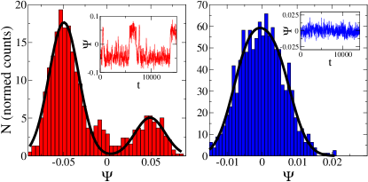
Figure S1: Method for determining throughput. Left panel: a state with net throughput, in which the throughput direction switches. The red bins show the normalized histogram of $\Psi(t)$, the solid black line is a fit using two Gaussians at $\pm\mu_{\Psi}$. In this example, the positive throughput state lasted for shorter simulation time, hence the difference in heights (means and standard deviations are the same). Both peaks will tend to the same height in the limit $t\to\infty$. Here $\zeta=5$, $\Delta=3.2\times 10^{-4}$, $\tau_{C}=1$. Right panel: a state with no net throughput for comparison, with $\zeta=5$, $\Delta=10^{-5}$, $\tau_{C}=1$. Insets: Examples of throughput-time series for each run.

We define the throughput as

$$\Psi(t)=\frac{1}{L_{y}}\int_{0}^{L_{y}}v_{x}(t)dy=\langle v_{x}(t)\rangle_{y}\;.$$ (S31)

As this quantity generally exhibits significant fluctuations in time, particularly in the chaotic regime, we additionally introduce a criterion for ‘net’ throughput, corresponding to the situation where the mean $\mu_{\Psi}$ of the throughput histogram exceeds the standard deviation $\sigma_{\Psi}$. These quantities are calculated using a least-squares fit of the throughput histograms with two Gaussians of width $\sigma_{\Psi}$, centered at $\pm\mu_{\Psi}$ . Examples of both throughput and non-throughput states are given in shown in Fig. S1.

References

- (1) M. C. Marchetti, J.-F. Joanny, S. Ramaswamy, T. B. Liverpool, J. Prost, M. Rao, and R. A. Simha, Rev. Mod. Phys. 85, 1143 (2013).
- (2) C. Dombrowski, L. Cisneros, S. Chatkaew, R. E. Goldstein, and J. O. Kessler, Phys. Rev. Lett. 93, 098103 (2004).
- (3) F. J. Nédélec, T. Surrey, A. C. Maggs, and S. Leibler, Nature 389, 305 (1997).
- (4) T. Sanchez, D. T. N. Chen, S. J. DeCamp, M. Heymann, and Z. Dogic, Nature 491, 431 (2012).
- (5) S. M. Fielding, D. Marenduzzo, and M. E. Cates, Phys. Rev. E 83, 041910 (2011).
- (6) H. H. Wensink, J. Dunkel, S. Heidenreich, K. Drescher, R. E. Goldstein, H. Löwen, and J. M. Yeomans, Proc. Natl. Acad. Sci. USA. 109, 14308 (2012).
- (7) L. Giomi, M. J. Bowick, X. Ma, and M. C. Marchetti, Phys. Rev. Lett. 110, 228101 (2013).
- (8) L. Giomi, M. J. Bowick, P. Mishra, R. Sknepnek, and M. C. 347 Marchetti, Phil. Trans. R. Soc. A 372, 20130365 (2014)
- (9) S. P. Thampi, R. Golestanian and J. M. Yeomans, Phys. Rev. Lett. 111, 118101 (2013).
- (10) S. Ramaswamy, Annu. Rev. Condens. Matt. Phys. 1, 323 (2010).
- (11) R. Voituriez, J.-F. Joanny, and J. Prost, Europhys. Lett. 70, 404 (2005).
- (12) R. A. Simha and S. Ramaswamy, Phys. Rev. Lett. 89, 058101 (2002).
- (13) A.N. Beris and B.J. Edwards, Thermodynamics of Flowing Systems, Oxford University Press, Oxford, (1994).
- (14) By contrast actomyosin systems, including the cytoskeleton, are typically contractile and polar; see F. Jülicher, K. Kruse, J. Prost, and J.-F. Joanny, Phys. Rep. 449, 3 (2007).
- (15) A. C. Callan-Jones and F. Jülicher, New J. Phys. 13, 093027 (2011) consider true multicomponent active gels, but do not explore rheology. A related but distinct combination of activity and viscoelasticity has been used to address tissue dynamics; see J.-F. Joanny and J. Prost, Seminaire Poincare XII 1-31 (2009); J. Ranft, M. Basan, J. Elgeti, J.-F. Joanny, J. Prost and F. Jülicher, Proc. Nat. Acad. Sci. USA 107, 20683 (2010). See also C. Storm, J. J. Pastore, F. C. MacKintosh, T. C. Lubensky, and P. A. Janmey, Nature 435, 191 (2005), for work addressing nonlinear polymer elasticity in active matter without direct construction of a coupled model; and see Contrary below for a study along similar lines to ours but addressing individual active particles, not an active nematic continuum, within a linear viscoelastic medium.
- (16) Y. Bozorgi and P. T. Underhill, J. Rheol. 57, 511 (2013).
- (17) A. W. Decho, Oceanogr. Mar. Biol. Annu. Rev 28, 73 (1990).
- (18) E. J. Hemingway, M. E. Cates and S. M. Fielding, in preparation.
- (19) Reversing the order of indices in would require sign reversal of wherever it appears.
- (20) S. T. Milner, Phys. Rev. E 48, 3674 (1993).
- (21) See Supplemental Material below or at http://link.aps.org/supplemental/10.1103/PhysRevLett.114.098302, which describes the free energy structure; enumerates all possible leading order active terms; and outlines the stability analysis and throughput definition that we adopt. This includes Refs. marend2007 ; Lu ; brand ; bertin .
- (22) D. Marenduzzo, E. Orlandini, and J. M. Yeomans, Phys. Rev. Lett. 98, 118102 (2007).
- (23) P.D. Olmsted and C.-Y. D. Lu, Phys Rev E 60, 4397 (1999).
- (24) H. Pleiner, M. Liu and H.R. Brand, Rheol Acta 41, 375 (2002).
- (25) E. Bertin, H. Chate, F Ginelli, S. Mishra, A. Peshkov and S. Ramaswamy et al., New J Phys 15 (2013) 085032.
- (26) P. D. Olmsted, O. Radulescu and C.-Y. D. Lu, J. Rheol. 44, 257, (2000)
- (27) G. Jayaraman, S. Ramachandran, S. Ghose, A. Laskar, M. S. Bhamla, P. B. S. Kumar and R. Adhikari, Phys. Rev. Lett. 109, 158302 (2012).
- (28) H. Stark and T. C. Lubensky, Phys. Rev. E: Stat., Nonlinear, Soft Matter Phys. 67, 061709 (2003)
- (29) The colon in (5) denotes contraction over second and third cartesian indices.
- (30) P. D. Olmsted, private communication.
- (31) H. C. Öttinger, Beyond Equilibrium Thermodynamics, Wiley, New York (2004).
- (32) M. Warner and E. M. Terentjev, Liquid Crystal Elastomers, Oxford University Press, Oxford (2002).
- (33) M. E. Cates, S. M. Fielding, D. Marenduzzo, E. Orlandini, and J. M. Yeomans, Phys. Rev. Lett. 101, 068102 (2008).
- (34) S. A. Edwards and J. M. Yeomans, Europhys. Lett. 85, 18008 (2009).
- (35) L. Giomi, L. Mahadevan, B. Chakraborty and M. F. Hagen, Nonlinearity 24, 2245 (2012).
- (36) C. M. White and M. G. Mungal, Annu. Rev. Fluid Mech. 40, 235 (2008).
- (37) See Supplemental Material at http://link.aps.org/supplemental/10.1103/PhysRevLett.114.098302 for movies of flowing states, showing principle eigenvalue of (colour scale), director (red lines), and defects (green/red circles).
- (38) S. P. Thampi, R. Golestanian and J. M. Yeomans, EPL 105, 18001 (2014).
- (39) S. Banerjee, A. Maitra, M. C. Marchetti, S. Ramaswamy, and J. Toner, in preparation.
- (40) For a somewhat similar situation involving polymer glasses, see S. M. Fielding, R. G. Larson, and M. E. Cates Phys. Rev. Lett. 108, 048301 (2012).
- (41) A. J. Bray, Adv. Phys. 43, 357 (1994).
- (42) Y. Bozorgi and P. T. Underhill J. Non-Newtonian Fluid Mech. 214, 69 (2014).

References

- (1) D. Marenduzzo, E. Orlandini, and J. M. Yeomans, Phys. Rev. Lett. 98, 118102 (2007).
- (2) P.D. Olmsted and C.-Y. D. Lu, Phys Rev E 60, 4397 (1999).
- (3) S. T. Milner, Phys. Rev. E 48, 3674 (1993).
- (4) H. Pleiner, M. Liu and H.R. Brand, Rheol Acta 41, 375 (2002).
- (5) A.N. Beris and B.J. Edwards, Thermodynamics of Flowing Systems, Oxford University Press, Oxford, (1994).
- (6) E. Bertin, H. Chate, F Ginelli, S. Mishra, A. Peshkov and S. Ramaswamy et al., New J Phys 15 (2013) 085032.