Integer percentages as electoral falsification fingerprints
Abstract
We hypothesize that if election results are manipulated or forged, then, due to the well-known human attraction to round numbers, the frequency of reported round percentages can be increased. To test this hypothesis, we analyzed raw data from seven federal elections held in the Russian Federation during the period from 2000 to 2012 and found that in all elections since 2004 the number of polling stations reporting turnout and/or leader’s result expressed by an integer percentage (as opposed to a fractional value) was much higher than expected by pure chance. Monte Carlo simulations confirmed high statistical significance of the observed phenomenon thereby suggesting its man-made nature. Geographical analysis showed that these anomalies were concentrated in a specific subset of Russian regions which strongly suggests its orchestrated origin. Unlike previously proposed statistical indicators of alleged electoral falsifications, our observations can hardly be explained differently but by a widespread election fraud.
keywords:
[class=MSC]keywords:
arXiv:1410.6059 \startlocaldefs \endlocaldefs
, and
1 Introduction
Human attraction to round numbers (such as e.g. multiples of 5 or 10) is a well-known psychological phenomenon, frequently observed e.g. in sports, examinations (Pope and Simonsohn, 2011), stock markets (Harris, 1991; Kandel, Sarig and Wohl, 2001; Osler, 2003), pricing (Klumpp, Brorsen and Anderson, 2005), tipping (Lynn, Flynn and Helion, 2013), census data (Yule, 1927), survey results (Crawford, Weiss and Suchard, 2014), etc. Excess of round numbers in such data is sometimes called “heaping” (Crawford, Weiss and Suchard, 2014). One likely interpretation of this phenomenon is that round numbers act as reference points when people are judging possible outcomes (Pope and Simonsohn, 2011). Recently, this phenomenon has helped catching data manipulations or forgery in cases of scientific misconduct (Simonsohn, 2013). Here we hypothesize that a similar effect could show up in electoral data as well: if election results are manipulated or forged, then the frequency of reported round percentages should be increased. To test this hypothesis, we analyzed raw data from seven federal elections held in the Russian Federation during the period from 2000 to 2012 and compared it to similar elections in other countries.
Russia presents an unusual case of a country where all raw electoral data are freely available for inspection, but election results are allegedly subject to forgery. Indeed, Russian federal elections after the year 2000 have often been accused of numerous falsifications, in particular on the grounds of multiple anomalies in the raw election data (Mikhailov, 2004; Mebane, 2006; Myagkov, Ordeshook and Shakin, 2009; Mebane and Kalinin, 2010; Klimek et al., 2012; Simpser, 2013; Ziegler, 2013; Enikolopov et al., 2013). Convincing as these indictments are, they all have serious limitations: some are indirect (Mikhailov, 2004; Myagkov, Ordeshook and Shakin, 2009) or model-based (Klimek et al., 2012), while the reported anomalies can in principle be explained by social, geographical or other confounding factors (Coleman, 2004; Churov, Arlazarov and Soloviev, 2008; Hansford and Gomez, 2010). Some are based on field experiments (Enikolopov et al., 2013) conducted in one single city; some rely on Benford’s law (Mebane, 2006; Mebane and Kalinin, 2010), were criticized for that (Deckert, Myagkov and Ordeshook, 2011), and are now deemed inconclusive (Mebane, 2013a, b; Mack and Shikano, 2013). The position of Russian authorities has always been that the official results of all Russian elections are genuine111Press conference of Vladimir Putin, 2011: http://www.rg.ru/2011/12/15/stenogramma.html (in Russian); Interview with the press attache for the president, Dmitry Peskov, 2011: http://lenta.ru/news/2011/12/12/noeffect (in Russian)..
Here we focus on another statistical anomaly: elevated frequency of round percentages in the election results. Anomalously high incidence of multiple-of-five percentages in some Russian federal elections has been observed before by one of us (as reported in Buzin and Lubarev, 2008, p 201), used in our preliminary work (Kobak, Shpilkin and Pshenichnikov, 2012), and also mentioned by Mebane et al. (Mebane and Kalinin, 2009, 2014; Kalinin and Mebane, 2010; Mebane, 2013b). Here we demonstrate that it is only a part of a more general phenomenon: anomalously high incidence of high integer percentages. We used Monte Carlo simulations to confirm statistical significance of this anomaly and measure its size. We argue that it presents a convincing evidence of election fraud that was absent in 2000 and 2003 federal elections, appeared in 2004 and has remained ever since.
2 Materials and methods
2.1 Background
Our analysis involves seven Russian federal elections: four presidential (2000, 2004, 2008, and 2012) and three legislative ones (2003, 2007, 2011). In each of these elections, the winner was either Vladimir Putin (2000, 2004, 2012) or his protégé Dmitry Medvedev (2008), or the pro-government party United Russia (2003, 2007, 2011). We always refer to the winner candidate or party as “leader”.
The legislative elections in 2007 and 2011 were conducted under a nationwide proportional system (i.e. the seats in the parliament were distributed between parties according to the proportion of votes for each party). The 2003 legislative election was mixed, with half of the deputies elected in a nationwide proportional election and another half in majoritarian districts (with each district electing one member of parliament); here we consider only the proportional part. The presidential elections are direct (i.e. people vote directly for the candidates and not for the electors as is the case in indirect elections), and in all elections under consideration the winner was determined in the first round, although the second round was in principle possible.
The total number of registered voters in Russia in 2000–2012 was about 108 million (107.2 to 109.8 million for different elections), and the total number of polling stations varied from to . At a lower level, the polling stations are grouped into constituencies (2744 to 2755 in total) corresponding to administrative territorial division. Constituencies vary in size and may contain from a few to more than a hundred polling stations. Constituency-level electoral commissions gather voting data in the form of paper protocols from the polling stations and enter them into the nationwide computerized database (“GAS Vybory”).
At a higher level, in 2012 Russia was divided into 83 federal regions. The number of regions slightly decreased from 2000 to 2012, as several regions were merged. In our analysis of earlier elections we combined the regions that would later be merged officially to keep consistency with the 2012 nomenclature.
2.2 Data
The raw election data with detalization to polling stations are officially published at the website of Russian Central Election Committee (izbirkom.ru) as multiple separate HTML pages and Excel reports. For our analysis, these data were downloaded with custom software scripts to form a joint database. The accuracy of the resulting databases was verified by checking regional subtotals and comparing a number of randomly chosen polling stations with the respective information at the official website. The parts of election databases relevant for the current study are provided as Supplementary Materials.
For the 2003–2012 elections, detailed data are available for each and every polling station in the country. For the 2000 election, the polling station level data are missing for the Republics of Chechnya and Sakha-Yakutia, and for several constituencies in other regions; available data cover polling stations (95% of total number) and 105.6 million voters (97.3% of total number).
For each polling station the following values (among many more) are available: the number of registered voters, the number of given ballots222This is the sum of ballots given to the voters at the polling station at the election day, ballots given to the voters outside of the polling station at the election day (in Russia it is possible to vote at home), and ballots given during early voting., the number of cast ballots (sum of valid and invalid ballots), and the number of ballots cast for the leader. In some cases, is not equal to due to taken away (not cast into the box) ballots; this fraction is small, 0.1–0.3%. According to Russian electoral laws333Federal law regulating parliamentary elections: http://cikrf.ru/law/federal_law/zakon_51/gl11.html., turnout at a given polling station is defined as % and leader’s result as %. Although turnout lost its legal significance after 2006 electoral law amendments that abolished turnout thresholds, de facto it is still customarily included in high-level official reports and, as our analysis will show, remains an important reporting figure at lower levels of the electoral system.
In special cases where is not defined beforehand (e.g. in temporary polling stations located at the train stations or airports), is officially reported as equal to , automatically resulting in 100% turnout (3–5% of all stations). We exclude all such stations from our analysis.
Official election results are reported at the national level only and are calculated as % and % for turnout and result, respectively. Although the results at lower levels (region, constituency, polling station) do not have any legal significance, they are nevertheless available at the Central Election Committee official website down to single polling station level.
2.3 Data from other countries
We used election data from three countries besides Russia: 2011 general election in Spain, 2010 presidential election in Poland (1st round), and 2009 federal election in Germany (Zweitstimmen, i.e. party votes). These three elections were chosen because the data are publicly available down to the single polling station level, and because the number and size of polling stations are comparable to those in Russia. The winners of these elections were the People’s Party, Bronisław Komorowski, and the CDU/CSU coalition respectively.
The Polish dataset is directly available at the official website in CSV format (prezydent2010.pkw.gov.pl), and the dataset for Spain is provided at the official website (www.infoelectoral.mir.es) in a custom format that requires decoding. The German dataset in CSV format was obtained by post on a CD after a request to the German federal returning officer (bundeswahlleiter.de).
In all cases is the number of registered voters and is the number of ballots cast for the leader. In Spain is defined as the sum of invalid, empty, and valid cast ballots and as the sum of empty and valid cast ballots. In Germany is defined as the sum of invalid and valid cast ballots and as the number of valid ballots. In Poland is defined as the number of given ballots and as the number of valid cast ballots.
The total number of polling stations is for Poland, for Spain, and for Germany (in Germany we excluded from the total number of stations those of them lacking information about the number of registered voters).
3 Results
3.1 Integer anomaly
To avoid any a priori assumptions about what constitutes a “round” percentage (multiple of 10? multiple of 5? any even number?), we chose to look at all integer percentages. As it is often impossible to achieve an exactly integer percentage at a given polling station because voter and ballot counts are integer (e.g. on a polling station with 974 registered voters the closest possible value to 70% turnout is 70.02% with 682 people participating in the election), we counted as integer all percentage values deviating from an integer by at most 0.05 percentage points. With characteristic number of ballots per station being 1000, such precision could almost always be achieved.
For each year we counted the number of polling stations where either turnout or leader’s result were given by an integer percentage (Figure 1A, dots); we will call those “integer polling stations”. Prior to this counting, we excluded all polling stations with turnout or result being over 99% because a large number of stations are reported with a formal turnout of 100% which is an integer; we wish to exclude these from the analysis (see Section 2.2). All polling stations with less than 100 registered voters were excluded as well because those are often temporary polling stations with some special status. The number of integer polling stations among the remaining stations is our main statistic.

One could think that in a fair election the chance for the turnout to be given by an integer is , and the same is true for the leader’s result; it follows that should be approximately equal to . However, the distribution of is affected by the distribution of polling station sizes: e.g. at a polling station with 100 registered people, all possible turnouts are integer. In particular for small polling stations the probability of can noticeably deviate from 0.19. For that reason we used Monte Carlo simulation to sample from the null distribution of .
Specifically, Monte Carlo simulations were based on the following null hypothesis: first, the election outcome at each polling station represents the true average intentions of voters at that particular location, and second, each person at each polling station votes freely and independently. Accordingly, for each polling station we modeled the turnout as a random variable
and the leader’s result as a random variable
Note that for large and this yields the following Gaussian approximation (not used in actual simulations):
meaning that e.g. for a polling station with 1000 registered voters and 60% turnout .
After generating and for all , the main statistic was computed as described above, and this procedure was repeated times to obtain values of sampled from the null distribution (a typical run of Monte Carlo iterations took 8h on a single core of an Intel i7 3.2 GHz processor). As a result, for each year we obtained a distribution of the amount of integer polling stations that could have arisen purely by chance, under the null hypothesis of no manipulations (Figure 1A, box plots).
Figure 1A shows that in 2000 and 2003 the empirical number of integer polling stations (computed from the actual electoral data) falls well within the 99% percentile interval of the Monte Carlo values. However, starting from 2004, the empirical number by far exceeds all Monte Carlo values, meaning that the observed number of integer polling stations could almost certainly not have occurred by chance. Therefore, the null hypothesis of no manipulations of the electoral results can be rejected with . Figure 1B shows how much the number of integer polling stations in each year exceeded the mean Monte Carlo value (i. e. the most likely value in the absence of manipulations): starting with 2004, the resulting “anomaly” is around 1000 polling stations, and it peaks in 2008 reaching almost 2000 polling stations.
The exact size of the anomaly depends on the window size used to define what percentage values are counted as being close enough to an integer. However, the anomaly sizes remain almost the same with windows ranging from around size (used above) to around , and the -scores peak around as shown on Figure 1C. Larger windows yield smaller and less significant anomalies (see also Figure 6 below), dropping to zero at window that simply counts all polling stations and therefore yields .
3.2 Controls
We ran a number of controls to ensure that the integer anomaly is a real and nontrivial effect.
First, the same anomaly can be computed for turnout and leader’s result separately. In both cases, the number of integer polling stations is well above the whole Monte Carlo range, as before (Figure 2A–B).
Second, one can worry that high number of integer polling stations can arise in fair elections due to artifacts of division of small integers (Johnston, Schroder and Mallawaaratchy, 1995) (even though small polling stations with less than 100 registered voters were excluded from our analysis). This cannot be so, because the same artifacts would then also appear in Monte Carlo simulations and would not make the empirical number of integer polling stations appear exceptional. Still, in addition to counting integer polling stations, we also computed the sum of registered voters at all integer polling stations (Figure 2C–D). This metric is mostly influenced by large polling stations. Significant and substantial anomalies in all years after 2004 confirm our conclusions and indicate that the integer anomaly is not an effect of small stations.
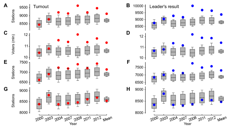
Third, it has been proposed before (Beber and Scacco, 2012) that a higher than expected number of polling stations reporting round (i.e. ending in 0) counts of registered voters, cast ballots, etc., can be taken as an evidence of fraud. Nonetheless, one can argue that such round counts can occur due to “innocent” (but still illegal) rounding in the exhausting manual ballot counting and do not necessarily imply a malicious fraud. Crucially, this is not the case for the anomaly reported here because the official precinct paper protocols in Russia contain only ballot counts, and do not contain either turnout or leader’s result in percent. However, the performance of a ballot station is likely to be judged by higher authorities by the shown percentages, prompting to fiddle with the ballot counts until appealing percentages are obtained. Notably, in most cases this requires non-round ballot counts. We have checked consistency of this argument by excluding all polling stations with round counts: the number of integer-turnout polling stations was computed without counting stations where either or ended on zero, and the number of integer-result polling stations was computed without counting stations where either or ended on zero (Figure 2E–F). This decreased the anomalous number of round percentages only slightly.
Fourth, we computed the number of polling stations with turnout or result differing by at most percentage points from a half-integer (as opposed to integer) percentage. This serves as a consistency check that, as expected, shows no significant effect in any year (Figure 2G–H).
Fifth, do our conclusions depend on the particular details of the Monte Carlo simulation? We argue that they do not. In addition to the binomial distribution, we also used the beta-binomial one:
This choice is motivated as follows. The observed turnout and leader’s result are not exact measurements of voters’ intentions, and one can estimate the conditional distribution of true voters’ intentions given the observed value and the uniform prior — this leads to the beta distribution. When a beta-distributed is used as a parameter for the binomial distribution, the compound distribution becomes beta-binomial. We performed beta-binomial Monte Carlo simulations (1000 iterations), and the null distributions hardly changed at all (Figure 1A).
Binomial distribution has been successfully used to describe statistics of election results across very different countries (Borghesi, Raynal and Bouchaud, 2012). For some countries, the data suggest that voters tend to vote in clusters, corresponding e.g. to families. This positive correlation between voters leads to higher variance of simulated outcomes at each polling station compared to the binomial distribution, and the integer percentages observed in the actual data would be smeared even stronger in the simulated data. To confirm this, we ran Monte Carlo simulations with various values of cluster sizes up to 10 and did not observe any excess of integer polling stations in the simulations.
The behaviour of actual voters is likely described by even more complex distributions, capturing perhaps some correlations between candidates and non-independence of voters. The existing evidence suggests that the more realistic distributions are overdispersed as compared to the binomial one (Borghesi, Raynal and Bouchaud, 2012). Whereas underdispersed distributions are theoretically possible, they seem unlikely to occur in real life (to yield noticeable underdispersion, voters should e.g. be precisely orchestrated or should en masse exhibit strong negative correlations). For these reasons we believe that the binomial assumption is conservative for the current purposes.
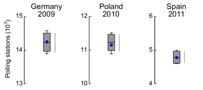
Finally, we applied our analysis to three recent elections outside Russia: one in Spain, one in Germany, and one in Poland. In each case we computed 1000 Monte Carlo iterations and in each case the number of integer polling stations was well inside the 99% percentile interval of the Monte Carlo values (Figure 3), demonstrating that the number of integer values was not at all anomalous. In fact, in each case the number of integer polling stations was very close to the mean Monte Carlo value, demonstrating adequacy of the model.
3.3 Specific integers
Which integer percentages contributed most to the integer anomaly? To answer this question, we considered histograms of turnout and leader’s result for each year (Figure 4). To account for different sizes of polling stations, we selected all polling stations exhibiting a particular turnout or leader’s result (in % bins) and plotted the total number of registered voters on these polling stations. The same histograms were computed for the surrogate data obtained with Monte Carlo simulations, and distributions of these surrogate histograms (99% percentile intervals) are shown on Figure 4 as gray shaded areas. Note that the Monte Carlo histograms follow the empirical ones very closely (except for a number of integer peaks, see below), demonstrating self-consistency of the Monte Carlo procedure.
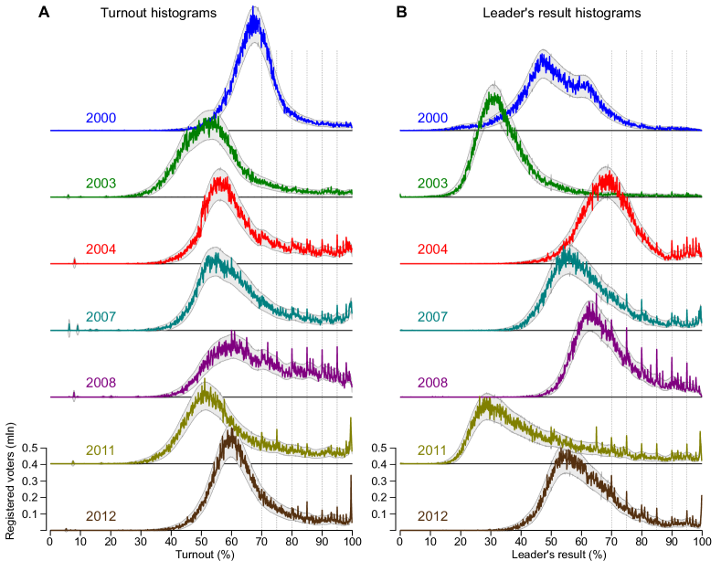
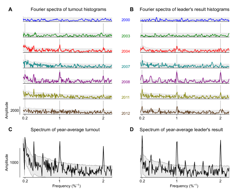
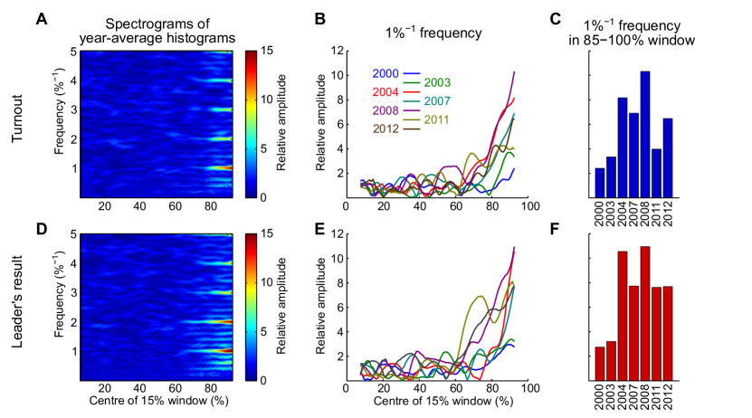
Starting from 2004, all empirical histograms exhibit pronounced sharp peaks at all integer percentage values of turnout and/or leader’s result above 70%. At multiples-of-five (75%, 80%, 85%, etc.) percentage values that are arguably more appealing, the peaks are particularly high (Buzin and Lubarev, 2008; Mebane and Kalinin, 2009). Nevertheless, smaller but denser peaks are also apparent at integer percentage values above 80% (e.g. at 91%, 92%, 93%, etc.). These peaks often reach well outside of the shaded Monte Carlo area, meaning that for many of them their individual -values are less than 0.0001. Fourier analysis confirms that the peaks are strictly equidistant with periods of 1% and 5% (Figure S1) and that such periodic peaks appear only at high percentages, namely above (Figure S2).
We carefully checked that these peaks are not the artifacts of division of small integers (Johnston, Schroder and Mallawaaratchy, 1995). Such artifacts can be observed in the election histograms if one chooses a very small bin size and counts polling stations directly instead of weighting them by registered voter counts (as we do). This allows small polling stations to contribute strongly to the distributions, leading to the artifact peaks at fractions with small denominators (such as 1/2, 2/3, 3/4, i.e. 50%, 66%, 75%). The peaks visible on Figure 4 are totally different from such artifacts, because (i) they are strictly periodic, (ii) they are never observed at 50% where the artifacts would be strongest, and (iii) they do not appear in Monte Carlo simulations that involve exactly the same type of integer divisions444A convenient way to get rid of such artifacts is to add a random number sampled from a uniform distribution to the nominator of each fraction, e.g. to the number of given ballots when computing the turnout. This does not noticeably influence the turnout value, but eliminates the problems associated with the division of integers. We did not apply this procedure here, as the artifacts were negligible..
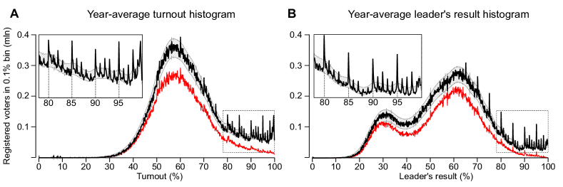
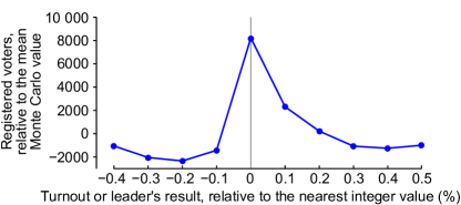
The integer peaks appear at the same positions in all years since 2004, demonstrating that the same integer numbers remain to be particularly appealing. Due to this fact, averaging the histograms over the years increases signal-to-noise ratio (Figure 5) allowing us to study the fine structure of the peaks. As can be seen in the insets of Figure 5, the peaks are asymmetric: sharp raising left flank is followed by a relaxed right tail.
To inspect this effect closer, we computed the average shape of all integer peaks in Figure 5. We subtracted the respective Monte Carlo mean values from the year-averaged turnout (Figure 5A) and leader’s result (Figure 5B) histograms, and averaged them over all 1%-long intervals around integer values (so the average was computed over 198 intervals, 99 for turnout and 99 for leader’s result, from 1% to 99%). Figure 6 confirms that the resulting shape is indeed asymmetric. This behavior is consistent with the interpretation that the polling station officials seem to be motivated to report a turnout or result which is “just above” an appealing integer value, rather than “just below” it. This leads to depletion of the votes right before an integer value, a peak at the exact integer value, and subsequent relaxation until the next integer value comes into play. This peculiar shape explains the decrease of -scores of the main anomaly as the window size around integer percentages gets too broad (Figure 1C).
3.4 Geographic distribution of integer anomaly
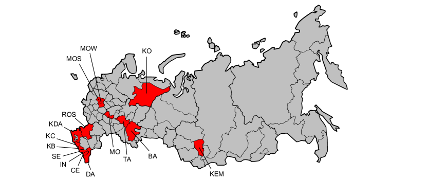
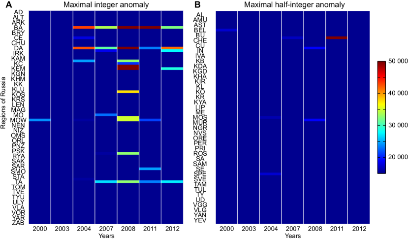
Geographically, polling stations contributing to the integer anomaly are not evenly distributed across Russia, but tend to cluster in certain regions. To show this, we computed the turnout and leader’s result histograms for each of the 7 elections in each of the 83 Russian regions separately and ranked the regions by the magnitude of the most conspicuous integer peak across years (Figure S3 and Table S4).
We found that the vast majority of the integer peaks originated from 15 regions, with the city of Moscow and the Moscow Region among them (Figure 7). If these 15 regions (comprising 33 mln voters, 30% of the national total) are excluded from the analysis, the integer peaks in both turnout and leader’s result histograms become negligibly small (Figure 5, red lines). Geographical clustering of integer polling stations strongly suggests that there existed tacit inducement, encouragement or even coordinating directives from the higher electoral commissions at the region level towards the individual polling stations (note that each region in Russia has its own electoral commission). Such conduct was rationalized by Kalinin and Mebane (2010) as regions signaling their loyalty to the center.
3.5 Relation to other electoral anomalies
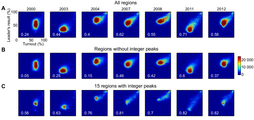
In a recent study (Klimek et al., 2012), two features of post-2004 Russian elections have been suggested as potential falsification fingerprints: high correlation between turnout and leader’s result, and high amount of polling stations with both turnout and leader’s result close to 100%. When the 15 aforementioned regions are excluded from the analysis, both features substantially weaken or disappear entirely.
This is illustrated by 2D histograms similar to the ones used in (Klimek et al., 2012) (Figure 8). Klimek et al. hypothesized that there are two main types of falsifications: “incremental fraud” when some extra ballots for the leader are added (ballot stuffing), and “extreme fraud” when a polling station reports almost 100% turnout and almost 100% leader’s result. On a 2D turnout-result histogram the first type of fraud shows as an extremely high correlation between turnout and leader’s result, while the second type of fraud gives rise to a separate second cluster near 100%-turnout, 100%-result point. Indeed, both features are present in Russian elections after 2004 (Figure 8A).
When the 15 regions demonstrating most prominent integer anomalies are excluded, the high-percentage cluster fully vanishes, and the correlation between turnout and leader’s result substantially weakens (Figure 8B). On the other hand, if only these 15 regions are used for the histograms, both anomalies become very prominent (Figure 8C).
The fact that the regions with the highest level of integer outcome anomaly are almost exactly those exhibiting other suspicious features, provides justification to the previous forensic methods (Mikhailov, 2004; Myagkov, Ordeshook and Shakin, 2009; Klimek et al., 2012; Simpser, 2013) and lends additional support to the current interpretation.
4 Conclusions
In sum, our results present a historical overview of the 2000–2012 Russian elections based on a novel statistical fraud indicator. The elections in 2000 and in 2003 do not appear to show any strong statistical anomalies. The anomalous integer-value peaks indicative of electoral manipulations popped up in 2004 and have persisted in the election data ever since, reaching a maximum in 2008 elections won by Dmitry Medvedev. What exactly happened during the three months between December 2003 and March 2004 when the respective elections were held, is an interesting politological question which however falls outside of the scope of the current paper. It remains to be seen if the anomalies discussed in this paper will show up in the upcoming 2016 parliament elections.
One of the limitations of the forensic method presented here is that it does not provide a way to estimate the overall impact of falsifications: not all ballots at dishonest polling stations are necessarily fraudulent, and not all dishonest polling stations report integer percentages. Nonetheless, agreement of our findings with the previous studies (Klimek et al., 2012) at the level of regions makes us believe that the excess of integer percentages is just a tip-of-the-iceberg effect unforeseen by the forgers. The real significance of the fraud indicator described herein is in its irrefutable character.
In a wider perspective, the methodology developed in this paper can also be useful for forensic studies of any datasets where percentages, or fractions, are of particular interest. Apart from the electoral data, this might be the case for scientific datasets where our method can possibly inform future investigations of scientific misconduct (Simonsohn, 2013).
Acknowledgements
We thank Sergey Slyusarev, Boris Ovchinnikov, Peter Klimek, and Uri Simonsohn for comments and suggestions, Alexey Shipilev for providing 2011–2012 election data on the fly, Alexander Shen for enlightening comments on statistical testing, and Günter Ziegler for providing us with the raw election data from Germany.
[id=suppA] \stitleElection data \slink[doi]https://dx.doi.org/10.6084/m9.figshare.3126883 \sdatatype.zip \sdescriptionDatasets used in this study (in tab-delimited plain text format).
References
- Beber and Scacco (2012) {barticle}[author] \bauthor\bsnmBeber, \bfnmBernd\binitsB. and \bauthor\bsnmScacco, \bfnmAlexandra\binitsA. (\byear2012). \btitleWhat the numbers say: A digit-based test for election fraud. \bjournalPolitical Analysis \bvolume20 \bpages211–234. \endbibitem
- Borghesi, Raynal and Bouchaud (2012) {barticle}[author] \bauthor\bsnmBorghesi, \bfnmChristian\binitsC., \bauthor\bsnmRaynal, \bfnmJean-Claude\binitsJ.-C. and \bauthor\bsnmBouchaud, \bfnmJean-Philippe\binitsJ.-P. (\byear2012). \btitleElection turnout statistics in many countries: similarities, differences, and a diffusive field model for decision-making. \bjournalPloS one \bvolume7 \bpagese36289. \endbibitem
- Buzin and Lubarev (2008) {bbook}[author] \bauthor\bsnmBuzin, \bfnmAndrei\binitsA. and \bauthor\bsnmLubarev, \bfnmArkadii\binitsA. (\byear2008). \btitleCrime without punishment (Prestuplenie bez nakazanija). \bpublisherMoscow: Nikkolo M. \endbibitem
- Churov, Arlazarov and Soloviev (2008) {binproceedings}[author] \bauthor\bsnmChurov, \bfnmV E\binitsV. E., \bauthor\bsnmArlazarov, \bfnmV L\binitsV. L. and \bauthor\bsnmSoloviev, \bfnmA V\binitsA. V. (\byear2008). \btitleItogi vyborov. Analiz elektoralnykh predpochtenij (Election outcome. Analysis of electoral preferences). In \bbooktitleTrudy instituta sistemnogo analiza Rossijskoj akademii nauk. Sbornik: matematika i upravlenie. \endbibitem
- Coleman (2004) {barticle}[author] \bauthor\bsnmColeman, \bfnmStephen\binitsS. (\byear2004). \btitleThe effect of social conformity on collective voting behavior. \bjournalPolitical analysis \bvolume12 \bpages76–96. \endbibitem
- Crawford, Weiss and Suchard (2014) {barticle}[author] \bauthor\bsnmCrawford, \bfnmForrest W\binitsF. W., \bauthor\bsnmWeiss, \bfnmRobert E\binitsR. E. and \bauthor\bsnmSuchard, \bfnmMarc A\binitsM. A. (\byear2014). \btitleSex, lies, and self-reported counts: Bayesian mixture models for longitudinal heaped count data via birth-death processes. \bjournalarXiv preprint arXiv:1405.4265. \endbibitem
- Deckert, Myagkov and Ordeshook (2011) {barticle}[author] \bauthor\bsnmDeckert, \bfnmJoseph\binitsJ., \bauthor\bsnmMyagkov, \bfnmMikhail\binitsM. and \bauthor\bsnmOrdeshook, \bfnmPeter C\binitsP. C. (\byear2011). \btitleBenford’s law and the detection of election fraud. \bjournalPolitical Analysis \bvolume19 \bpages245–268. \endbibitem
- Enikolopov et al. (2013) {barticle}[author] \bauthor\bsnmEnikolopov, \bfnmRuben\binitsR., \bauthor\bsnmKorovkin, \bfnmVasily\binitsV., \bauthor\bsnmPetrova, \bfnmMaria\binitsM., \bauthor\bsnmSonin, \bfnmKonstantin\binitsK. and \bauthor\bsnmZakharov, \bfnmAlexei\binitsA. (\byear2013). \btitleField experiment estimate of electoral fraud in Russian parliamentary elections. \bjournalProceedings of the National Academy of Sciences \bvolume110 \bpages448–452. \endbibitem
- Hansford and Gomez (2010) {barticle}[author] \bauthor\bsnmHansford, \bfnmThomas G\binitsT. G. and \bauthor\bsnmGomez, \bfnmBrad T\binitsB. T. (\byear2010). \btitleEstimating the electoral effects of voter turnout. \bjournalAmerican Political Science Review \bvolume104 \bpages268–288. \endbibitem
- Harris (1991) {barticle}[author] \bauthor\bsnmHarris, \bfnmLawrence\binitsL. (\byear1991). \btitleStock price clustering and discreteness. \bjournalReview of Financial Studies \bvolume4 \bpages389–415. \endbibitem
- Johnston, Schroder and Mallawaaratchy (1995) {barticle}[author] \bauthor\bsnmJohnston, \bfnmRoger G\binitsR. G., \bauthor\bsnmSchroder, \bfnmShayla D\binitsS. D. and \bauthor\bsnmMallawaaratchy, \bfnmA Rajika\binitsA. R. (\byear1995). \btitleStatistical artifacts in the ratio of discrete quantities. \bjournalThe American Statistician \bvolume49 \bpages285–291. \endbibitem
- Kalinin and Mebane (2010) {binproceedings}[author] \bauthor\bsnmKalinin, \bfnmKirill\binitsK. and \bauthor\bsnmMebane, \bfnmWalter R\binitsW. R. (\byear2010). \btitleUnderstanding Electoral Frauds through Evolution of Russian Federalism: from “Bargaining Loyalty” to “Signaling Loyalty”. In \bbooktitleAnnual Meeting of the American Political Science Association, Washington. \endbibitem
- Kandel, Sarig and Wohl (2001) {barticle}[author] \bauthor\bsnmKandel, \bfnmShmuel\binitsS., \bauthor\bsnmSarig, \bfnmOded\binitsO. and \bauthor\bsnmWohl, \bfnmAvi\binitsA. (\byear2001). \btitleDo investors prefer round stock prices? Evidence from Israeli IPO auctions. \bjournalJournal of banking & finance \bvolume25 \bpages1543–1551. \endbibitem
- Klimek et al. (2012) {barticle}[author] \bauthor\bsnmKlimek, \bfnmPeter\binitsP., \bauthor\bsnmYegorov, \bfnmYuri\binitsY., \bauthor\bsnmHanel, \bfnmRudolf\binitsR. and \bauthor\bsnmThurner, \bfnmStefan\binitsS. (\byear2012). \btitleStatistical detection of systematic election irregularities. \bjournalProceedings of the National Academy of Sciences \bvolume109 \bpages16469–16473. \endbibitem
- Klumpp, Brorsen and Anderson (2005) {binproceedings}[author] \bauthor\bsnmKlumpp, \bfnmJoni M\binitsJ. M., \bauthor\bsnmBrorsen, \bfnmB Wade\binitsB. W. and \bauthor\bsnmAnderson, \bfnmKim B\binitsK. B. (\byear2005). \btitleThe Preference for Round Number Prices. In \bbooktitleAnnual Meeting of the Southern Agricultural Economics Association, Little Rock, Arkansas \bvolume35537. \bpublisherSouthern Agricultural Economics Association. \endbibitem
- Kobak, Shpilkin and Pshenichnikov (2012) {barticle}[author] \bauthor\bsnmKobak, \bfnmDmitry\binitsD., \bauthor\bsnmShpilkin, \bfnmSergey\binitsS. and \bauthor\bsnmPshenichnikov, \bfnmMaxim S\binitsM. S. (\byear2012). \btitleStatistical anomalies in 2011-2012 Russian elections revealed by 2D correlation analysis. \bjournalarXiv preprint arXiv:1205.0741. \endbibitem
- Lynn, Flynn and Helion (2013) {barticle}[author] \bauthor\bsnmLynn, \bfnmMichael\binitsM., \bauthor\bsnmFlynn, \bfnmSean Masaki\binitsS. M. and \bauthor\bsnmHelion, \bfnmChelsea\binitsC. (\byear2013). \btitleDo consumers prefer round prices? Evidence from pay-what-you-want decisions and self-pumped gasoline purchases. \bjournalJournal of Economic Psychology \bvolume36 \bpages96–102. \endbibitem
- Mack and Shikano (2013) {binproceedings}[author] \bauthor\bsnmMack, \bfnmV\binitsV. and \bauthor\bsnmShikano, \bfnmS\binitsS. (\byear2013). \btitleBenford’s Law-test on trial. Simulation-based application to the latest election results from France and Russia. In \bbooktitleMeeting of the Midwest Political Science Association, Chicago. \endbibitem
- Mebane (2006) {binproceedings}[author] \bauthor\bsnmMebane, \bfnmWalter R\binitsW. R. (\byear2006). \btitleElection forensics: Vote counts and Benford’s law. In \bbooktitleSummer Meeting of the Political Methodology Society, UC-Davis. \endbibitem
- Mebane (2013a) {binproceedings}[author] \bauthor\bsnmMebane, \bfnmWalter R\binitsW. R. (\byear2013a). \btitleElection Forensics: The Meanings of Precinct Vote Counts’ Second Digits. In \bbooktitleSummer Meeting of the Political Methodology Society, UC-Davis. \endbibitem
- Mebane (2013b) {binproceedings}[author] \bauthor\bsnmMebane, \bfnmWalter R\binitsW. R. (\byear2013b). \btitleUsing Vote Counts’ Digits to Diagnose Strategies and Frauds: Russia. In \bbooktitleAnnual Meeting of the American Political Science Association. \endbibitem
- Mebane and Kalinin (2009) {binproceedings}[author] \bauthor\bsnmMebane, \bfnmWalter R\binitsW. R. and \bauthor\bsnmKalinin, \bfnmKirill\binitsK. (\byear2009). \btitleComparative election fraud detection. In \bbooktitleAnnual Meeting of the American Political Science Association, Toronto. \endbibitem
- Mebane and Kalinin (2010) {binproceedings}[author] \bauthor\bsnmMebane, \bfnmWalter R\binitsW. R. and \bauthor\bsnmKalinin, \bfnmKirill\binitsK. (\byear2010). \btitleElectoral fraud in Russia: vote counts analysis using second-digit mean tests. In \bbooktitleAnnual Meeting of the Midwest Political Science Association, Chicago. \endbibitem
- Mebane and Kalinin (2014) {binproceedings}[author] \bauthor\bsnmMebane, \bfnmWalter R\binitsW. R. and \bauthor\bsnmKalinin, \bfnmKirill\binitsK. (\byear2014). \btitleGeography in Election Forensics. In \bbooktitleAnnual Meeting of the American Political Science Association. \endbibitem
- Mikhailov (2004) {bincollection}[author] \bauthor\bsnmMikhailov, \bfnmValentin\binitsV. (\byear2004). \btitleRegional elections and democratization in Russia. In \bbooktitleRussian politics under Putin (\beditor\bfnmCameron\binitsC. \bsnmRoss, ed.) \bpages198–220. \bpublisherManchester University Press. \endbibitem
- Myagkov, Ordeshook and Shakin (2009) {bbook}[author] \bauthor\bsnmMyagkov, \bfnmMikhail\binitsM., \bauthor\bsnmOrdeshook, \bfnmPeter C\binitsP. C. and \bauthor\bsnmShakin, \bfnmDimitri\binitsD. (\byear2009). \btitleThe forensics of election fraud: Russia and Ukraine. \bpublisherCambridge University Press. \endbibitem
- Osler (2003) {barticle}[author] \bauthor\bsnmOsler, \bfnmCarol L\binitsC. L. (\byear2003). \btitleCurrency orders and exchange rate dynamics: an explanation for the predictive success of technical analysis. \bjournalThe Journal of Finance \bvolume58 \bpages1791–1820. \endbibitem
- Pope and Simonsohn (2011) {barticle}[author] \bauthor\bsnmPope, \bfnmDevin\binitsD. and \bauthor\bsnmSimonsohn, \bfnmUri\binitsU. (\byear2011). \btitleRound Numbers as Goals. Evidence From Baseball, SAT Takers, and the Lab. \bjournalPsychological science \bvolume22 \bpages71–79. \endbibitem
- Simonsohn (2013) {barticle}[author] \bauthor\bsnmSimonsohn, \bfnmUri\binitsU. (\byear2013). \btitleJust Post It. The Lesson From Two Cases of Fabricated Data Detected by Statistics Alone. \bjournalPsychological science \bvolume24 \bpages1875–1888. \endbibitem
- Simpser (2013) {bbook}[author] \bauthor\bsnmSimpser, \bfnmAlberto\binitsA. (\byear2013). \btitleWhy governments and parties manipulate elections: theory, practice, and implications. \bpublisherCambridge University Press. \endbibitem
- Yule (1927) {barticle}[author] \bauthor\bsnmYule, \bfnmG Udny\binitsG. U. (\byear1927). \btitleOn reading a scale. \bjournalJournal of the Royal Statistical Society \bpages570–587. \endbibitem
- Ziegler (2013) {bbook}[author] \bauthor\bsnmZiegler, \bfnmGünter M\binitsG. M. (\byear2013). \btitleMathematik — Das ist doch keine Kunst! \bpublisherAlbrecht Knaus Verlag. \endbibitem
Appendix A Supplementary figures
See next page.
| ISO code | Region name | Maximal integer anomaly () |
|---|---|---|
| DA | Dagestan, Respublika | 87 |
| BA | Bashkortostan, Respublika | 64 |
| KEM | Kemerovskaya Oblast | 52 |
| KDA | Krasnodarskiy Krai | 51 |
| KO | Komi, Respublika | 38 |
| MOS | Moskovskaya Oblast | 35 |
| MOW | Moscow | 34 |
| KB | Kabardino-Balkarskaya Respublika | 33 |
| TA | Tatarstan, Respublika | 33 |
| ROS | Rostovskaya Oblast | 33 |
| IN | Ingushetiya, Respublika | 28 |
| SE | Severanaya Osetiya-Alaniya, Respublika | 24 |
| MO | Mordoviya, Respublika | 23 |
| KC | Karachayevo-Cherkesskaya Respublika | 21 |
| CE | Chechenskaya Respublika | 18 |