The perils of thresholding

Abstract

The thresholding of time series of activity or intensity is frequently used to define and differentiate events. This is either implicit, for example due to resolution limits, or explicit, in order to filter certain small scale physics from the supposed true asymptotic events. Thresholding the birth-death process, however, introduces a scaling region into the event size distribution, which is characterised by an exponent that is unrelated to the actual asymptote and is rather an artefact of thresholding. As a result, numerical fits of simulation data produce a range of exponents, with the true asymptote visible only in the tail of the distribution. This tail is increasingly difficult to sample as the threshold is increased. In the present case, the exponents and the spurious nature of the scaling region can be determined analytically, thus demonstrating the way in which thresholding conceals the true asymptote. The analysis also suggests a procedure for detecting the influence of the threshold by means of a data collapse involving the threshold-imposed scale.

I Introduction

Thresholding is a procedure applied to (experimental) data either deliberately, or effectively because of device limitations. The threshold may define the onset of an event and/or an effective zero, such that below the threshold the signal is regarded as $0$. An example of thresholding is shown in Fig. 1. Experimental data often comes with a detection threshold that cannot be avoided, either because the device is insensitive below a certain signal level, or because the signal cannot be distinguished from noise. The quality of a measurement process is often quantified by the noise to signal ratio, with the implication that high levels of noise lead to poor (resolution of the) data. Often, the rationale behind thresholding is to weed out small events which are assumed irrelevant on large scales, thereby retaining only the asymptotically big events which are expected to reveal (possibly universal) large-scale physics.

Figure 1: Example of thresholding of a time series. An event begins when the signal exceeds the threshold (dotted lines, $h=10,20,30$) and ends as soon as the signal falls below the threshold. Increasing levels of the threshold lead (non-monotonically) to different numbers of events and, provided the signal eventually ends, monotonically smaller total event durations. The main focus of this paper is on the statistics of the individual event durations, as exemplified by the two intervals for the intermediate threshold.

Most, if not all, of physics is due to some basic interactions that occur on a “microscopic length scale”, say the interaction between water droplets or the van der Waals forces between individual water molecules. These length scales separate different realms of physics, such as between micro-fluidics and molecular physics or between molecular physics and atomic physics. However, these are not examples of the thresholds we are concerned with in the following. Rather, we are interested in an often arbitrary microscopic length scale well above the scale of the microscopic physics that governs the phenomenon we are studying, such as the spatiotemporal resolution of a radar observing precipitation (which is much coarser than the scale set by microfluidics), or the resolution of the magnetometer observing solar flares, (which is much coarser than the scale set by atomic physics and plasma magnetohydrodynamics).

Such thresholds often come down to the device limitations of the measuring apparatus, the storage facilities connected to it, or the bandwidth available to transmit the data. For example, the earthquake catalogue of Southern California is only complete above magnitude $3$, even though the detection-threshold is around magnitude $2$ Schorlemmer and Woessner (2008). One fundamental problem is the noise-to-signal ratio mentioned above. Even if devices were to improve to the level where the effect of noise can be disregarded, thresholding may still be an integral part of the measurement. For example, the distinction between rainfall and individual drops requires a separation of microscale and macroscale which can be highly inhomogeneous Lovejoy et al. (2003). Solar flares, meanwhile, are defined to start when the solar activity exceeds the threshold and end when it drops below, but the underlying solar activity never actually ceases Paczuski et al. (2005).

Thresholding has also played an important rôle in theoretical models, such as the Bak-Sneppen Model (Bak and Sneppen, 1993) of Self-Organised Criticality Pruessner (2012), where the scaling of the event-size distribution is a function of the threshold (Paczuski et al., 1996) whose precise value was the subject of much debate (Sneppen, 1995; Grassberger, 1995). Finite size effects compete with the threshold-imposed scale, which has been used in some models to exploit correlations and predict extreme events Garber et al. (2009).

Often, thresholding is tacitly assumed to be “harmless” for the (asymptotic) observables of interest and beneficial for the numerical analysis. We will argue in the following that this assumption may be unfounded: the very act of thresholding can distort the data and the observables derived from it. To demonstrate this, we will present an example of the effect of thresholding by determining the apparent scaling exponents of a simple stochastic process, the birth-death process (BDP). We will show that thresholding obscures the asymptotic scaling region by introducing an additional prior scaling region, solely as an artefact. Owing to the simplicity of the process, we can calculate the exponents, leading order amplitudes and the crossover behaviour analytically, in excellent agreement with simulations. In doing so, we highlight the importance of sample size since, for small samples (such as might be accessible experimentally), only the “spurious” threshold-induced scaling region that governs the process at small scales may be accessible. Finally, we discuss the consequences of our findings for experimental data analysis, where detailed knowledge of the underlying process may not be available, usually the mechanism behind the process of interest is unclear, and hence such a detailed analysis is not feasible. But by attempting a data collapse onto a scaling ansatz that includes the threshold-induced scale, we indicate how the effects of thresholding can be revealed.

(a)  Small sample size $\mathcal{N}=10^{3}$.

(b)  Large sample size $\mathcal{N}=10^{10}$.

Figure 2: 2(a): The PDF $\mathcal{P}^{{(g_{s})}}\left(g_{s};h\right)$ of the survival time $g_{s}$ of a thresholded BDP, with a threshold of $h=100$, estimated from Monte Carlo simulations using a limited sample size of $\mathcal{N}=10^{3}$. Fitting a power law yields an exponent of $\hat{\gamma}_{1}=1.52(3)$ over the range $[0.031,1.259\cdot 10^{5}]$ , with a $p$-value of 0.71. 2(b): Same as above, but using a sample size of $\mathcal{N}=10^{10}$. In this case, two power laws can be fitted in two different regimes: below $g_{\mathsf{X}}=8\pi h$, we find $\hat{\gamma}_{1}=1.50070(2)$ in the (fixed) range $[10^{-2},10^{3}]$, while above $g_{\mathsf{X}}$, the fit leads to $\hat{\gamma}_{2}=1.998(4)$ over the range $[1.99\cdot 10^{5},3.16\cdot 10^{8}]$ , with a p-value of 0.55. Monte Carlo simulations are shown as symbols, while the small (large) regime power-law fit is plotted with full black lines, and the fitted range marked with red (blue) shading.

The outline of the paper is as follows: In Sec. LABEL:sec:model we introduce the model and the thresholding applied to it. To illustrate the problems that occur when thresholding real data, we analyse in detail some numerical data. The artefact discovered in this analysis finds explanation in the theory present in Sec. LABEL:sec:results. We discuss these findings and suggest ways to detect the problem in the final section.

II Model

In order to quantify numerically and analytically the effect of thresholding, we study the birth-death Gardiner (1997) process (BDP) with Poissonian reproduction and extinction rates that are proportional to the population size. More concretely, we consider the population size $n(g)$ at (generational) time $g\geq 0$. Each individual in the population reproduces and dies with the same rate of $1/2$ (in total unity, so that there are $n(g)$ birth or death events or “updates” per time unit on average); in the former case (birth) the population size increases by $1$, in the latter (death) it decreases by $1$. The state $n(g)=0$ is absorbing Hinrichsen (2000). Because the instantaneous rate with which the population $n(g)$ evolves is $n(g)$ itself, the exponential distributions from which the random waiting times between events are drawn are themselves parameterised by a random variable, $n(g)$.

Because birth and death rates balance each other, the process is said to be at its critical point Harris (1963), which has the peculiar feature that the expectation of the population is constant in time, $\left\langle n(g)\right\rangle=n(g_{0})$, where $\left\langle\cdot\right\rangle$ denotes the expectation and $n(g_{0})$ is the initial condition, set to unity in the following. This constant expectation is maintained by increasingly fewer surviving realisations, as each realisation of the process terminates almost surely. We therefore define the survival time as the time $g_{s}-g_{0}$ such that $n(g)>0$ for all $g_{0}\leq g<g_{s}$ and $n(g)=0$ for all $g\geq g_{s}$. For simplicity, we may shift times to $g_{0}=0$, so that $g_{s}$ itself is the survival time. It is a continuous random variable, whose probability density function (PDF) is well known to have a power law tail in large times, $\mathcal{P}^{{(g_{s})}}\left(g_{s}\right)\propto g_{s}^{-2}$ (Harris, 1963, as in the branching process).

In the following, we will introduce a threshold, which mimics the suppression of some measurements either intentionally or because of device limitations. For the BDP this means that the population size (or, say, “activity”) below a certain, prescribed level, $h$, is treated as $0$ when determining survival times. In the spirit of (Peters et al., 2002, also solar flares, Paczuski et al., 2005), the threshold allows us to distinguish events, which, loosely speaking, start and end whenever $n(g)$ passes through $h$.

Explicitly, events start at $g_{0}$ when $\lim_{\epsilon\to 0^{+}}n(g_{0}-\epsilon)=h$ and $n(g_{0})=h+1$. They end at $g_{s}$ when $n(g_{s})=h$, with the condition $n(g)>h$ for all $g_{0}\leq g<g_{s}$. This is illustrated in Figs. 1 and 4. No thresholding takes place (i.e. the usual BD process is recovered) for $h=0$, in which case the initial condition is $n(g_{0})=1$ and termination takes place at $g_{s}$ when $n(g_{s})=0$. For $h>0$ one may think of $n(g)$ as an “ongoing” time series which never ceases and which may occasionally “cross” $h$ from below (starting the clock), returning to $h$ some time later (stopping the clock). In a numerical simulation one would start $n(g)$ from $n(g_{0})=h+1$ at $g_{0}=0$ and wait for $n(g)$ to arrive at $n(g)=h$ from above. The algorithm may be summarised as

for $i=1\dots\mathcal{N}$ do

     $n\leftarrow h+1$

     $g_{i}\leftarrow 0$

     while $n>h$ do

         $g_{i}\leftarrow g_{i}+\xi(n)$

         $n\leftarrow n+b$

     end while

end for

where $\xi(n)$ is an exponential random variable with rate $n$, and $b$ stands for a random variable that takes the values $\{-1,1\}$ with probability 1/2. In our implementation of the algorithm, all random variables are handled with the GNU Scientific Library (Galassi et al., 2009).

II.1 Numerics and data analysis

Monte-Carlo runs of the model reveal something unexpected: The exponent of the PDF of the thresholded BDP appears to change from $\mathcal{P}^{{(g_{s})}}\left(g_{s}\right)\propto g_{s}^{-2}$ at $h=0$ to $\mathcal{P}^{{(g_{s})}}\left(g_{s}\right)\propto g_{s}^{-3/2}$ at $h=100$ or, in fact, any reasonably large $h\gtrsim 10$. Fig. 2 shows $\mathcal{P}^{{(g_{s})}}\left(g_{s}\right)$ for the case of $h=100$ and two different sample sizes, $\mathcal{N}_{1}=10^{3}$ and $\mathcal{N}_{2}=10^{10}$, corresponding to “scarce data” and “abundant data”, respectively. In the former case, the exponent of the PDF is estimated to be $\hat{\gamma}_{1}=1.52(3)\approx 3/2$; in the latter, the PDF splits into two scaling regimes, with exponents $\hat{\gamma}_{1}=1.50070(2)\approx 3/2$ and $\hat{\gamma}_{2}=1.998(4)\approx 2$. This phenomenon can be investigated systematically for different sample sizes $\mathcal{N}$ and thresholds $h$.

We use the fitting procedure introduced in Deluca and Corral (2013), which is designed not only to estimate the exponent, but to determine the range in which a power law holds in an objective way. It is based on maximum likelihood methods, the Kolmogorov-Smirnov test and Monte Carlo simulations of the distributions. In Fig. 3 we show the evolution of the estimated large scale exponent, $\hat{\gamma}_{2}$, for different $\mathcal{N}$ and for different $h$. The fits are made by assuming that there is a true power law in a finite range [a,b]. For values of the exponent between 1.5 and 2 larger error bars are observed. For these cases, less data is fitted but the fitting range is always at least two orders of magnitude wide.

It is clear from Fig. 3 that $\mathcal{N}$ has to be very large in order to see the true limiting exponent. Even the smallest $h$ investigated, $h=20$, needs a sample size of at least $\mathcal{N}=10^{7}$, while for $h=5\,000$ the correct exponent is not found with less than about $\mathcal{N}=10^{10}$.

The mere introduction of a threshold therefore changes the PDF of events sizes significantly. It introduces a new, large scaling regime, with an exponent that is misleadingly different from that characterising large scale asymptotics. In fact, for small sample sizes ($\mathcal{N}_{1}=10^{3}$, see Fig. 2(a)), the only visible regime is that induced by thresholding (in our example, $\gamma_{1}=3/2$), while the second exponent ($\gamma_{2}=2$), which, as will be demonstrated below, governs the large scale asymptotics, remains hidden unless much larger sample sizes are used (Fig. 2(b)).

Although the algorithm is easy to implement, finding the two scaling regimes numerically can be challenging. There are a number of caveats:

1. The crossover point $g_{\mathsf{X}}$ between the two scaling regimes scales linearly with the threshold, $g_{\mathsf{X}}=8\pi h$ (see Sec. LABEL:sec:distribution_of_gs), effectively shifting the whole $g_{s}^{-2}$ asymptotic regime to larger and thus less likely values of $g_{s}$. To maintain the same number of events above $g_{\mathsf{X}}\propto h$, one needs $\mathcal{N}\int_{g_{\mathsf{X}}}^{\infty}\mathchoice{\!\mathrm{d}g_{s}\,}{\!\mathrm{d}g_{s}\,}{\!\mathrm{d}g_{s}\,}{\!\mathrm{d}g_{s}\,}g_{s}^{-2}=\text{const}$, i.e. $\mathcal{N}\propto h$.

2. Because the expected running time of the algorithm diverges, one has to set an upper cutoff on the maximum generational timescale, say $g_{s}<G$. If the computational complexity for each update is constant, an individual realisation, starting from $n(0)=h+1$ and running up to $n(g_{s})=h$ with $g_{s}<G$, has complexity $\mathcal{O}(g_{s}^{2})$ in large $g_{s}$ where $g_{s}^{2}$ is the scaling of the expected survival time of the mapped random walker introduced below. The expected complexity of realisations that terminate before $G$ (with rate $\sim 1/g_{s}^{2}$) is therefore linear in $G$, $\int_{1}^{G}\mathchoice{\!\mathrm{d}g_{s}\,}{\!\mathrm{d}g_{s}\,}{\!\mathrm{d}g_{s}\,}{\!\mathrm{d}g_{s}\,}g_{s}^{-2}g_{s}^{2}=G-1$. With the random walker mapping it is easy to see that the expected population size $n(g)$ of realisations that terminate after $G$ (and therefore have to be discarded as $g_{s}$ exceeds $G$) is of the order $n(g_{s})\sim G$ for $g_{s}=G$. These realisations, which appear with frequency $\propto 1/G$, have complexity $\mathcal{O}(G^{2})$, i.e. the complexity of realisations of the birth-death process is $\mathcal{O}(G)$ both for those counted into the final tally and those dismissed because they exceed $G$. There is no point probing beyond $G$ if $\mathcal{N}$ is too small to produce a reasonable large sample on a logarithmic scale, $\mathcal{N}\int_{G}^{2G}\mathchoice{\!\mathrm{d}g_{s}\,}{\!\mathrm{d}g_{s}\,}{\!\mathrm{d}g_{s}\,}{\!\mathrm{d}g_{s}\,}g_{s}^{-2}=\text{const}$, so that $\mathcal{N}\sim G$ and thus the overall complexity of a sample of size $\mathcal{N}$ is $\mathcal{O}(\mathcal{N}^{2})$ and thus $\mathcal{O}(h^{2})$ for $G\sim g_{\mathsf{X}}\sim h$ and $\mathcal{N}\propto h$ from above.

That is, larger $h$ necessitates larger $\mathcal{N}$, leading to quadratically longer CPU time. In addition, parallelisation of the algorithm helps only up to a point, as the (few) biggest events require as much CPU time as all the smaller events taken together. The combination of all these factors has the unfortunate consequence that, for large enough values of $h$, observing the $\mathcal{P}^{{(g_{s})}}\left(g_{s}\right)\propto g_{s}^{-2}$ regime is simply out of reach (even for moderate values of $h$, such as $h=100$, to show the crossover as clearly as in Fig. 2, a sample size as large as $\mathcal{N}=9\cdot 10^{9}$ was necessary, which required about 1810 hours of CPU time).

Figure 3: Estimated large scale exponent $\hat{\gamma}_{2}$ for different thresholds $h$ and sample size $\mathcal{N}$. The error bars correspond to one standard deviation and are inversely proportional to the number of data within the fitted range.

III Results

While it is straightforward to set up a recurrence relation for the generating function if the threshold is $h=0$, the same is not true for $h>0$. This is because the former setup ($h=0$) does not require an explicit implementation of the absorbing wall since the process terminates naturally when $n(g)=0$ (there is no individual left that can reproduce or die). If, however, $h>0$, the absorbing wall has to be treated explicitly and that is difficult when the evolution of the process (the effective diffusion constant) is a function of its state, i.e. the noise is multiplicative. In particular, a mirror charge trick cannot be applied.

Figure 4: Magnification of the right interval in Fig. 1. The clock starts when $n(g)$ exceeds the threshold and stops when $n(g)$ returns to the threshold.

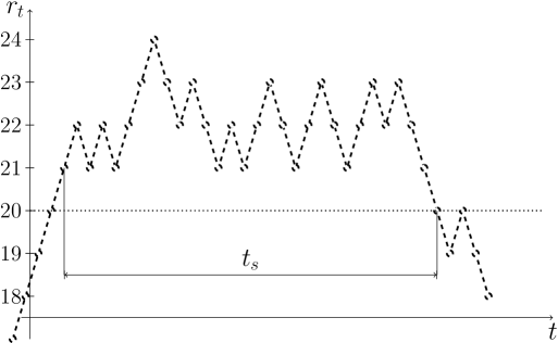
Figure 5: The same data as in Fig. 4 but on the mapped time scale of the random walker, which evolves in equally spaced, discrete steps. The survival time is necessarily odd, $t_{s}=2T-1$, $T\in\mathds{N}$ ($t_{s}=29$ in this example).

However, the process can be mapped to a simple random walk by “a change of clocks”, a method detailed in Rubin et al. (2014). For the present model, we observe that $n(g)$ performs a fair random walk $r_{t}$ by a suitable mapping of the generational timescale $g$ to that of the random walker, $r_{t}(g)=n(g)$ with $t(g)\in\mathds{N}$. In fact, because of the Poissonian nature of the BD process, birth and death almost surely never occur simultaneously and a suitable, unique $t(g)$ is found by $t(0)=0$ and

$$\lim_{\epsilon\to 0^{+}}t(g+\epsilon)-t(g-\epsilon)=\lim_{\epsilon\to 0^{+}}|n(g+\epsilon)-n(g-\epsilon)|$$ (1)

i.e. $t(g)$ increases whenever $n(g)$ changes and is therefore an increasing function of $g$. With this map, $r_{t}$ is a simple random walk along an absorbing wall at $h$, see Fig. 5. The challenge is to derive the statistics of the survival times $g_{s}$ on the time scale of the BD process from the survival times $t_{s}$ on the time scale of the random walk.

In the following, we first approximate some important properties of the survival times in a handwaving manner before presenting a mathematically sound derivation in Sec. LABEL:sec:maths.

III.1 Approximation

The expected waiting time between two events in the BDP is $1/n$, if $n$ is the current population size, with $n=n_{x}+h$ such that $n_{x}$ is the excess of $n$ above $h$. As discussed in detail in Sec. LABEL:sec:maths, $n_{x}$ is a time-dependent random variable, and so taking the ensemble average of the waiting time is a difficult task. But on the more convenient time scale $t$, the excess $n_{x}$ performs a random walk and it is in that ensemble, with that time scale, where we attempt to find the expectation

$$\overline{g_{s}(t_{s};h)}=\sum_{t=0}^{t_{s}-1}\left\langle\frac{1}{n_{x}(t)+h}\right\rangle_{\mathcal{R}(t_{s})}\ ,$$ (2)

which is the expected survival time of a thresholded BD process given a certain return (or survival) time $t_{s}$ of the random walker. In this expression $n_{x}(t)$ is a time-dependent random variable and the ensemble average $\left\langle\cdot\right\rangle_{\mathcal{R}(t_{s})}$ is taken over all random walker trajectories $\mathcal{R}(t_{s})$ with return time $t_{s}$. To ease notation, we will include the argument of $\mathcal{R}(t_{s})$ only where necessary. Approximating the random variable $g_{s}$ by its mean $\overline{g_{s}(t_{s};h)}$ given in Eq. (2) and approximated further below affords an approximate map of the known PDF $\mathcal{P}^{{(t_{s})}}\left(t_{s}\right)$ of $t_{s}$ to the PDF $\mathcal{P}^{{(g_{s})}}\left(g_{s}\right)$ of $g_{s}$,

$$\mathcal{P}^{{(g_{s})}}\left(g_{s}\right)\frac{\mathrm{d}}{\mathrm{d}t_{s}}\overline{g_{s}(t_{s};h)}\approx\mathcal{P}^{{(t_{s})}}\left(t_{s}\right)$$ (3)

This map will be made rigorous in Sec. LABEL:sec:maths, avoiding the use of $\overline{g_{s}(t_{s};h)}$ in lieu of the random variable.

In a more brutal approach, one may approximate the time dependent excess $n_{x}(t)$ in Eq. (2) by its expectation conditional to a certain survival time $t_{s}$,

$$\left\langle\frac{1}{h+n_{x}(t)}\right\rangle_{\mathcal{R}}=\frac{1}{h+\left\langle n_{x}(t)\right\rangle_{\mathcal{R}}}\left\langle\frac{1}{1+\frac{n_{x}(t)-\left\langle n_{x}(t)\right\rangle_{\mathcal{R}}}{h+\left\langle n_{x}(t)\right\rangle_{\mathcal{R}}}}\right\rangle\\ =\frac{1}{h+\left\langle n_{x}(t)\right\rangle_{\mathcal{R}}}+\text{(higher order terms)}$$ (4)

so that the expected survival time $g_{s}(t_{s})$ given a certain return time $t_{s}$ is approximately $t_{s}/(h+\left\langle n_{x}(t)\right\rangle_{\mathcal{R}})$.

The quantity $\left\langle n_{x}(t)\right\rangle_{\mathcal{R}}$ is the expected excursion of a random walker, which is well-known to be

$$\left\langle n_{x}(t)\right\rangle_{\mathcal{R}}\approx\sqrt{\frac{\pi}{8}}t_{s}^{1/2}$$ (5)

in the continuum limit (with diffusion constant $1/2$) (e.g. Majumdar and Comtet, 2004, 2005). Thus,

$$\overline{g_{s}(t_{s};h)}\approx\frac{t_{s}}{h+\sqrt{\pi t_{s}/8}}\ .$$ (6)

At small times, $h\gg\sqrt{\pi t_{s}/8}$, the relation between $g_{s}$ and $t_{s}$ is essentially linear, $g_{s}\approx t_{s}/h$, whereas for large times, $h\ll\sqrt{\pi t_{s}/8}$, the asymptote is $g_{s}\approx\sqrt{8t_{s}/\pi}$. Writing the right-hand-side of Eq. (6) in the form $\sqrt{8t_{s}/\pi}\frac{1}{1+\sqrt{8h^{2}/(\pi t_{s})}}$ allows us to extract the scaling of the crossover time. The argument of the square root is of order unity when $t_{{\mathsf{X}}}=8h^{2}/\pi$, for which $g_{s}(t_{{\mathsf{X}}},h)\approx 4h/\pi$. Moreover, one can read off the scaling form

$$\overline{g_{s}(t_{s};h)}\approx t_{s}^{1/2}\mathcal{G}(t_{s}/h^{2})\ ,$$ (7)

with $\mathcal{G}(x)=\sqrt{8/\pi}/(1+\sqrt{8/(\pi x)})$ and asymptotes $\mathcal{G}(x)\approx\sqrt{x}$ for small $x$ and $\lim_{x\to\infty}\mathcal{G}(x)=\sqrt{8/\pi}$.

The PDF of the survival time

$$\mathcal{P}^{{(t_{s})}}\left(t_{s}\right)=\frac{1}{\sqrt{4\pi Dt}}\frac{a}{Dt_{s}}\mathchoice{e^{-\frac{a^{2}}{4Dt_{s}}}}{\operatorname{exp}\left(-\frac{a^{2}}{4Dt_{s}}\right)}{\operatorname{exp}\left(-\frac{a^{2}}{4Dt_{s}}\right)}{\operatorname{exp}\left(-\frac{a^{2}}{4Dt_{s}}\right)}$$ (8)

of a random walker along an absorbing wall is well-known to be a power law $\propto t_{s}^{-3/2}$ for times $t_{s}$ large compared to the time scale set by the initial condition, i.e. the distance $a$ of the random walker from the absorbing wall at time $t=0$. The precise value of $a$ is effectively determined by the details the continuum approximation, here $a=1$, $D=1/2$, and so we require $1\ll 2t_{s}$.

To derive the PDF of the BD process, note that Eq. (6) has the unique inverse $t_{s}(g_{s})=\frac{\pi g_{s}^{2}}{16}\mathcal{T}(\frac{16h}{\pi g_{s}})$, where $\mathcal{T}(y)=1+y+\sqrt{1+2y}$. Evaluating the crossover time by setting $y=1$ yields $g_{{\mathsf{X}}}=16h/\pi$. The PDF of the survival time of the BD process finally reads

$$\mathcal{P}^{{(g_{s})}}\left(g_{s};h\right)\sim\left(\frac{\pi}{16}\mathcal{T}(y)\right)^{-1/2}g_{s}^{-2}\left(2-\frac{y\mathcal{T}^{\prime}(y)}{\mathcal{T}(y)}\right)$$ (9)

where $y=\frac{16h}{\pi g_{s}}$. For small $y$, the last bracket converges to $2$, so $\mathcal{P}^{{(g_{s})}}\left(g_{s};h\right)\sim 2\sqrt{8/\pi}g_{s}^{-2}$ for large $g_{s}$. For large $y$, the last bracket converges to $1$, so $\mathcal{P}^{{(g_{s})}}\left(g_{s};h\right)\sim(1/\sqrt{h})g_{s}^{-3/2}$ for small $g_{s}$.

This procedure recovers the results in Sec. LABEL:sec:maths: For $g_{s}\ll 16h/\pi$ the PDF of the survival times in the BD process goes like $g_{s}^{-3/2}$, and for $g_{s}\gg 16h/\pi$ like $g_{s}^{-2}$, independent of $h$. Eq. (9) also gives a prescription for a collapse, since $\mathcal{P}^{{(g_{s})}}\left(g_{s};h\right)g_{s}^{2}$ plotted versus $g_{s}/h$ should, for sufficiently large $g_{s}$, reproduce the same curve, as confirmed in Fig. 7 and Fig. 8.

Applying a threshold introduces a new scale, $16h/\pi$, below which the PDF displays a clearly discernible power law, $g_{s}^{-3/2}$, corresponding to the return time of a random walker. The “true” $g_{s}^{-2}$ power law behaviour (the large $g_{s}$ asymptote) is visible only well above the threshold-induced crossover.

III.2 Detailed Analysis

In the previous section we made a number of assumptions, in particular the approximation of replacing the random variable by its expectation, and the approximation in Eq. (4), which both require further justification.

In the present section we proceed more systematically. In particular, we will be concerned with the statistics of the BD survival time $g_{s}(\mathcal{R})$ given a particular trajectory $\mathcal{R}=\{r_{0},r_{1},\ldots,r_{t_{s}}\}$ of the random walk, where $t_{s}=2T-1$, necessarily odd, $T\in\mathds{N}$, see Figs. 5 and 9. We will then relax the constraint of the trajectory and study the whole ensemble $\Omega$ of random walks terminating at a particular time $2T-1$, denoting as $g_{s}(\Omega(T))$ a survival time drawn from the distribution of all survival times of a BD process with a mapping to a random walker that terminates at $2T-1$ or, for simplicity, just $g_{s}(\Omega)$. This will allow us to determine the existence of a limiting distribution for $g_{s}(\Omega)/\sqrt{T}$ and to make a quantitative statement about its mean and variance. We will not make any assumptions about the details of that limiting distribution; in order to determine the asymptotes of $\mathcal{P}^{{(g_{s})}}\left(g_{s};h\right)$ we need only know that the limit exists.

For a given trajectory $\mathcal{R}$ of the random walk, the resulting generational survival time $g_{s}(\mathcal{R})$ may be written as

$$g_{s}(\mathcal{R})=\sum_{t=0}^{2T-2}\xi_{t}(r_{t}+h),$$ (10)

where $\xi_{t}(\alpha)$ is a random variable drawn at time $t$ from an exponential distribution with rate $\alpha$, i.e. drawn from $\alpha\mathchoice{e^{-\alpha\xi}}{\operatorname{exp}\left(-\alpha\xi\right)}{\operatorname{exp}\left(-\alpha\xi\right)}{\operatorname{exp}\left(-\alpha\xi\right)}$, and $r_{t}$ is the position of the random walk at time $t$, with initial condition $r_{0}=1$ and terminating at $2T-1$ with $r_{2T-1}=0$ (see Fig. 9).

The mean and standard deviation of $\xi_{t}$ are $1/(r_{t}+h)$, necessarily finite, so that by the central limit theorem the limiting distribution of $g_{s}(\mathcal{R})/\sqrt{T}$ given a trajectory $\mathcal{R}$ is Gaussian (for $T\gg 1$). This ensures that $g_{s}(\Omega)/\sqrt{T}$ has a limiting distribution (see Appendix LABEL:sec:limiting_dist).

It is straightforward to calculate the mean and standard deviation of $g_{s}(\mathcal{R})$ for a particular trajectory $\mathcal{R}$ that terminates after $2T-1$ steps. Slightly more challenging is the mean $\mu(\Omega)$ and variance $\sigma^{2}(\Omega)$ of $g_{s}(\Omega)$ for the entire ensemble $\Omega$ of such trajectories. The details of this calculation are relegated to Appendix LABEL:sec:mean_var_appendix. Here, we state only the key results. For the mean of the survival time, we find

$$\mu(\Omega)\simeq 2\sqrt{\pi T}+2h\psi\left(\frac{h}{\sqrt{T}}\right)$$ (11)

(see Eq. (41)) with $\psi(x)=\mathchoice{e^{-x^{2}}}{\operatorname{exp}\left(-x^{2}\right)}{\operatorname{exp}\left(-x^{2}\right)}{\operatorname{exp}\left(-x^{2}\right)}(\operatorname{Ei}(x)-\pi\mathcal{E}(\imath x)/\imath)$ and asymptotes

$$\mu(\Omega)\simeq 2\sqrt{\pi T} T\gg h^{2}$$ for (12a)

$$\mu(\Omega)\simeq 2T/h T\ll h^{2}$$ for (12b)

see Eq. (43b). The variance is

$$\sigma^{2}(\Omega)\simeq T\ \mathcal{I}(x)-\mu(\Omega)^{2}+\mathcal{K}(x)$$ (13)

(see Eq. (46)) with integrals $\mathcal{I}(x)$ and $\mathcal{K}(x)$ defined in Eq. (47) and with asymptotes

$$\sigma^{2}(\Omega)\simeq 4\pi T\frac{\pi-3}{3} T\gg h^{2}$$ for (14a)

$$\sigma^{2}(\Omega)\simeq 2T/h^{2} T\ll h^{2}$$ for  , (14b)

see Eq. (51b). All these results are derived in the limit $T\gg 1$ in which the mapped random walker takes more than just a few steps, corresponding to a continuum approximation. However, as shown in the following, the results remain valid even for $T$ close to one.

To assess the quality of the continuum approximation and the validity of the asymptotes, we extracted the mean $\mu(\Omega(T))$ and variance $\sigma^{2}(\Omega(T))$ of the survival time $g_{s}(\Omega(T))$ from simulated BDPs starting with a population size $n(0)=h+1$ and returning to $n(g_{s})=h$ after $2T-1$ updates (births or deaths), i.e. the process was conditioned to a particular value of $T$. In particular, we set the threshold at $h=100$, and simulated a sample of $10^{5}$ constrained BDPs for values $T=2^{k},k=0\dots 20$. The results are shown in Fig. 6 and confirm the validity of the large $T\gg 1$ approximation in Eq. (11) and Eq. (13), as well as the asymptotes Eq. (12b) and Eq. (14b). Remarkably, as previously stated, Eq. (11) and Eq. (13) are seen to be valid even when the condition $T\gg 1$ does not reasonably hold.

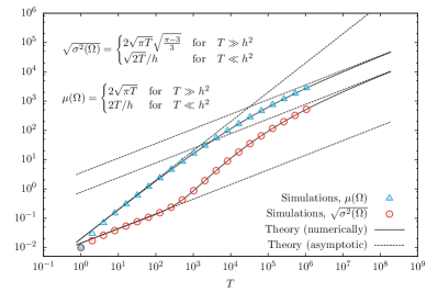
Figure 6: Numerical comparison of the approximations Eq. (11) and Eq. (13) (shown as full lines), their asymptotes Eq. (12b) and Eq. (14b) (dashed) and the numerical estimates based on a sample of $10^{5}$ realisations per datapoint in a Monte-Carlo simulation of a birth-death process constrained to $2T-1$ updates, with $h=100$ and $T=2^{k},k=0\dots 20$.

III.2.1 Distribution of $g_{s}$

For large $T$, the generational survival time $g_{s}$ given a survival time $2T-1$ of the mapped random walk has PDF

$$\mathcal{P}^{{(g_{s})}}\left(g_{s};h;T\right)\simeq\frac{1}{\sqrt{\sigma^{2}(\Omega(T))}}\Phi\left(\frac{g_{s}-\mu(\Omega(T))}{\sqrt{\sigma^{2}(\Omega(T))}}\right),$$ (15)

where $\Phi(x)$ denotes the limiting distribution of the rescaled survival time $(g_{s}-\mu(\Omega(T)))/\sqrt{\sigma^{2}(\Omega(T)})$, and the mean $\mu(\Omega(T))$ and variance $\sigma^{2}(\Omega(T))$ are given by Eq. (11) and Eq. (13). We demonstrate that $\Phi$ exists and find its precise (non-Gaussian) form in Appendix LABEL:sec:limiting_dist for completeness, but we will not use this result in what follows: to extract the asymptotic exponents and first order amplitudes, see below, knowledge of the mean $\mu(\Omega)$ and variance $\sigma^{2}(\Omega)$ is sufficient.

As the ensembles $\Omega(T)$ are disjoint for different $T$, the overall distribution $\mathcal{P}^{{(g_{s})}}\left(g_{s};h\right)$ of survival generational times is therefore given by the sum of the constrained distribution $\mathcal{P}^{{(g_{s})}}\left(g_{s};h;T\right)$ weighted by the probability of the mapped random walk to terminate after $2T-1$ steps. In the limit of large $T$, as assumed throughout, that weight is $T^{-3/2}/(2\sqrt{\pi})$ (Mohanty, 1979). Therefore,

$$\mathcal{P}^{{(g_{s})}}\left(g_{s};h\right)=\sum_{T=1}^{\infty}\frac{T^{-3/2}}{2\sqrt{\pi}}\frac{1}{\sqrt{\sigma^{2}(\Omega(T))}}\Phi\left(\frac{g_{s}-\mu(\Omega(T))}{\sqrt{\sigma^{2}(\Omega(T))}}\right).$$ (16)

To extract asymptotic behaviour for $T\ll h^{2}$ and $T\gg h^{2}$ we make a crude saddle point, or “pinching” approximation, by assuming that $\Phi(x)$ essentially vanishes for $|x|>1/2$ and is unity otherwise. This fixes the random walker time $T$ via $g_{s}-\mu(\Omega(T))=0$, while the number of terms in the summation is restricted to satisfy $|g_{s}-\mu(\Omega(T))|\leq\sqrt{\sigma^{2}(\Omega(T))}$. After some algebra we find

$$\mathcal{P}^{{(g_{s})}}\left(g_{s};h\right)= \frac{h+1}{2} g_{s}\ll 1/h$$ ​​ for (17a)

$$\mathcal{P}^{{(g_{s})}}\left(g_{s};h\right)= \frac{g^{-3/2}}{\sqrt{2\pi h}} 1/h\ll g_{s}\ll 8\pi h$$ ​​ for (17b)

$$\mathcal{P}^{{(g_{s})}}\left(g_{s};h\right)= 2g^{-2} g_{s}\gg 8\pi h$$ ​​ for (17c)

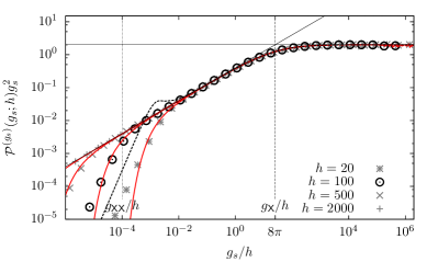
Figure 7: Collapse of the PDFs for different thresholds $h$ for large $g_{s}\gg 1/h$, plotting $\mathcal{P}^{{(g_{s})}}\left(g_{s};h\right)g_{s}^{2}$ against $g_{s}/h$, according to Eq. (9) and Eq. (18), capturing Eq. (17b) and Eq. (17c). The black full lines indicate the asymptotes according to Eq. (17c), the dashed lines show the crossovers at $g_{s}/h=8\pi$ and $g_{s}/h=1/h^{2}$ for $h=100$ . Finally, the black thick dashed line corresponds to the analytical solution computed from Eq. (16) for $h=100$, while the red full lines were computed by numerically inverting the Laplace transform given in Eq. (70), see Appendix LABEL:sec:laplace_transform. Another collapse is possible according to Eq. (19).

The qualitative scaling of these two asymptotes was anticipated after Eq. (9). The crossover time $g_{{\mathsf{X}}}=8\pi h$, shown in Figs. 7 and 8, can be determined by assuming continuity of $\mathcal{P}^{{(g_{s})}}\left(g_{s};h\right)$ and thus imposing $\frac{1}{\sqrt{2h\pi}}g_{{\mathsf{X}}}^{-3/2}=2g_{{\mathsf{X}}}^{-2}$. Fig. 7 shows $\mathcal{P}^{{(g_{s})}}\left(g_{s};h\right)g_{s}^{2}$ versus $g_{s}/h$ for varying $h$, comparing Monte Carlo simulations for varying $h$ with the numerical evaluation of Eq. (16) for $h=100$, thus confirming the validity of the data collapse proposed in Eq. (9). In particular, the shape of the transition between the two asymptotic regimes, predicted to take place near $g_{\mathsf{X}}/h=8\pi$, is recovered from Eq. (16) with great accuracy. As an alternative to the numerical evaluation of Eq. (16), we introduce in Appendix LABEL:sec:laplace_transform a complementary approach that provides the Laplace transform of $\mathcal{P}^{{(g_{s})}}\left(g_{s};h\right)$, see Eq. (70). Unfortunately, inverting the Laplace transform analytically does not seem feasible, but numerical inversion provides a perhaps simpler means of evaluating $\mathcal{P}^{{(g_{s})}}\left(g_{s};h\right)$ in practice.

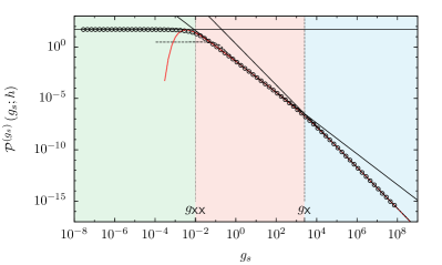
Figure 8: The PDF of survival times $\mathcal{P}^{{(g_{s})}}\left(g_{s};h\right)$ for $h=100$. Three scaling regimes partitioned by $g_{\mathsf{X}}$ (thin dashed line) and $g_{{\mathsf{X}}{\mathsf{X}}}$ (thin dotted line) exist: For very short times $g_{s}\ll 1/h$ (green shading), the exponential waiting time to the first (death) event dominates, so that $\mathcal{P}^{{(g_{s})}}\left(g_{s};h\right)\sim(h+1)/2$. For “intermediate” times (red shading) $1/h\ll g_{s}\ll 8\pi h$, the effect of the threshold dominates, and hence $\mathcal{P}^{{(g_{s})}}\left(g_{s};h\right)\sim g_{s}^{-3/2}/\sqrt{2\pi h}$. For long times (blue shading) $g_{s}\gg 8\pi h$, $\mathcal{P}^{{(g_{s})}}\left(g_{s};h\right)\sim 2g_{s}^{-2}$, independently of $h$. Monte-Carlo simulation results are shown as symbols, asymptotes of $\mathcal{P}^{{(g_{s})}}\left(g_{s};h\right)$, Eq. (17c), as solid lines, and the analytical solution $\mathcal{P}^{{(g_{s})}}\left(g_{s};h\right)$, computed via Eq. (16) as a black thick dashed line, and via numerical inversion of the Laplace transform, Eq. (70), as a red solid line.

In addition to the two asymptotic regimes discussed so far, one notices that Fig. 8 displays yet another “regime” (left-most, green shading), which corresponds to extremely short survival times. This regime is almost exclusively due to the walker dying on the first move via the transition $n(0)=h+1$ to $n(g_{s})=h$. In this case, the sum in Eq. (10) only has one term, and hence the PDF of $g_{s}$ can be approximated as $\mathcal{P}^{{(g_{s})}}\left(g_{s};h\right)=\frac{1}{2}(h+1)\mathchoice{e^{-(h+1)g_{s}}}{\operatorname{exp}\left(-(h+1)g_{s}\right)}{\operatorname{exp}\left(-(h+1)g_{s}\right)}{\operatorname{exp}\left(-(h+1)g_{s}\right)}\sim\frac{h+1}{2}$, where the factor $1/2$ corresponds to the probability of $T=1$, and the limit of small $g_{s}$ has been taken. Thus, for very short times $g_{s}\ll 1/h$, the PDF of $g_{s}$ is essentially “flat”. In order to estimate the transition point to this third regime, we impose again continuity of the solution, so that $(h+1)/2=g_{{{\mathsf{X}}{\mathsf{X}}}}^{-3/2}/\sqrt{2\pi h}$ and hence (dropping the constants) $g_{{{\mathsf{X}}{\mathsf{X}}}}=1/h$, as shown in Eq. (17c) as well as Figs. 7 and 8.

Given the three regimes shown in Fig. 7, $\mathcal{P}^{{(g_{s})}}\left(g_{s};h\right)$ can be collapsed either by ignoring the very short scale, (see Eq. (9))

$$\mathcal{P}^{{(g_{s})}}\left(g_{s};h\right)\simeq 2g_{s}^{-2}\mathcal{G}_{>}(g_{s}/h)\qquad\text{for}\qquad g\gg 1/h$$ (18)

with $\mathcal{G}_{>}(x)=1$ for large $x$ and $\mathcal{G}_{>}(x)=\sqrt{x/(8\pi)}$ in small $x$, or according to

$$\mathcal{P}^{{(g_{s})}}\left(g_{s};h\right)\simeq\frac{g_{s}^{-3/2}}{\sqrt{2\pi h}}\mathcal{G}_{<}(g_{s}h)\qquad\text{for}\qquad g\ll 8\pi h$$ (19)

with $\mathcal{G}_{<}(x)=1$ for large $x$ and $\mathcal{G}_{<}(x)=x^{3/2}\sqrt{\pi/2}$ for small $x$. Power-law scaling (crossover) functions offer a number of challenges, as they affect the “apparent” scaling exponent (Christensen et al., 2008). Also, there is no hard cutoff in the present case, i.e. moments $\left\langle g_{s}^{m}\right\rangle=\int\mathchoice{\!\mathrm{d}g_{s}\,}{\!\mathrm{d}g_{s}\,}{\!\mathrm{d}g_{s}\,}{\!\mathrm{d}g_{s}\,}\mathcal{P}^{{(g_{s})}}\left(g_{s};h\right)g_{s}^{m}$ do not exist for $m\geq 2$.

IV Discussion

The main goal of the present paper has been to understand how thresholding influences data analysis. In particular, how thresholding can change the scaling of observables and how one might detect this.

To this end, we worked through the consequences of thresholding in the birth-death process, which is known to have a power-law PDF of survival times with exponent $\gamma=2$. We have shown, both analytically and via simulations, that the survival times $g_{s}$ for the thresholded process include a new scaling regime with exponent $\gamma=3/2$ in the range $1/h\ll g_{s}\ll 8\pi h$ (see Fig. 8), where $h$ is the intensity level of the threshold.

We would like to emphasise how difficult it is to observe the asymptotic $\gamma=2$ exponent, even for such an idealized toy model. For large values of the threshold, $h=5\,000$, sample sizes as large as $10^{10}$ are needed in order to populate the histogram for large survival times. Real-world measurements are unlikely to meet the demand for such vast amounts of data. An illustration of what might then occur for realistic amounts of data that are subject to threshold is given by Fig. 2, where only the threshold-induced scaling regime associated with exponent $-3/2$ is visible.

Intriguingly, a qualitatively similar scaling phenomenology is observed in renormalised renewal processes with diverging mean interval sizes Corral (2009). The random deletion of points (that, together with a rescaling of time, constitutes the renormalisation procedure) is analogous to the raising of a threshold. It can be shown that the non-trivial fixed point distribution of intervals is bi-power law. The asymptotic scaling regime has the same exponent as that of the original interval sizes. But, in addition, a prior scaling regime emerges with a different exponent, and the crossover separating the two regimes moves out with increasing threshold.

A fundamental difference between theoretical models and the analysis of real-world processes is that in the former, asymptotic exponents are defined in the limit of large events, with everything else dismissed as irrelevant, whereas real world phenomena are usually concerned with finite event sizes. In our example, the effect of the threshold dominates over the “true” process dynamics in the range $1/h\ll g_{s}\ll 8\pi h$, and grows with increasing $h$ before eventually taking over the whole region of physical interest.

Of course, real data may not come from an underlying BDP. But we believe that the specific lessons of the BDP apply more generally to processes with multiplicative noise, i.e. a noise whose amplitude changes with the dynamical variable (the degree of freedom): At large thresholds small changes of that variable are negligible and an effectively additive process is obtained (the plain random walker above). Only for large values of the dynamical variable is the original process recovered. These large values are rare, in particular when another cutoff (such as, effectively, the sample size) limits the effective observation time ($2T-1$ above). In this context it is worth mentioning the work of Laurson et al. Laurson et al. (2009), in which thresholds were applied to Brownian excursions. However, since noise is additive in Brownian motion, the effect of thresholding is relatively benign. Indeed, no new scaling regime appears as a result of thresholding, and the asymptotic exponent of $-3/2$ is recovered no matter what threshold is applied.

In the worst case, thresholding may therefore bury the asymptotics which would only be recovered for much longer observation times. However, if the threshold can easily be changed, its effect can be studied systematically by attempting a data collapse onto the scaling ansatz $\mathcal{P}^{{(g_{s})}}\left(g_{s};h\right)=g_{s}^{-\gamma}\mathcal{G}(g_{s}/h^{D})$, Eqs. (9) and (18), with exponents $\gamma$ and $D$ to be determined, as performed in Fig. 7 with $\gamma=2$ and $D=1$. The threshold plays an analogous rôle to the system size in finite-size scaling (albeit for intermediate scales). In the present case, the exponents in the collapse, together with the asymptote of the scaling function, identify two processes at work, namely the BDP as well as the random walk.

Appendix A Mean and variance of the survival time

This appendix contains the details of the calculations leading to the approximation (in large $T$), Eq. (11) and Eq. (13), as well as their asymptotes Eq. (12b) and Eq. (14b), for the mean $\mu(\Omega)$ and the variance $\sigma^{2}(\Omega)$ respectively, averaged over the ensemble $\Omega(T)$, or $\Omega$ for short, of the mapped random walks with the constraint that they terminate at $2T-1$, see Fig. 9.

Figure 9: Sample path of a random walk along an absorbing wall at $0$. The walker starts at $t=0$ from $r_{0}$ and terminates at $2T-1$ by reaching the wall $r_{2T-1}=0$, i.e. $r_{2T-2}=1$. By construction, it cannot escape from the region demarcated by the dashed line. When counting distinct paths, the number of paths terminating at $r_{2T-1}=0$ equals the number of paths passing through $r_{2T-2}=1$.

In the following, we will use the notation $\xi_{t}$ for $\xi_{t}(r_{t}+h)$, but it is important to note that any two $\xi_{t}(r_{t}+h)$ are independent, even though the consecutive $r_{t}$ are not. The random variable $g_{s}(\mathcal{R})$ in Eq. (10) is thus a sum of independent random variables $\xi_{t}$, whose mean and variance at consecutive $t$, however, are correlated due to $r_{t}$ being a trajectory of a random walk. Because $h+r_{t}>0$ for $t<2T-1$, the limiting distribution of $(g_{s}(\mathcal{R})-\mu(\mathcal{R}))/\sqrt{\sigma^{2}(\mathcal{R})}$ as $T\to\infty$ is a Gaussian with unit variance. Mean $\mu(\mathcal{R})$ and variance $\sigma^{2}(\mathcal{R})$ are defined as

$$\mu(\mathcal{R}) = \left\langle g_{s}(\mathcal{R})\right\rangle_{\mathcal{R}}=\sum_{t=0}^{2T-2}\left\langle\xi_{t}\right\rangle_{\mathcal{R}}$$ (20a)

$$\sigma^{2}(\mathcal{R}) = \left\langle(g_{s}(\mathcal{R}))^{2}\right\rangle_{\mathcal{R}}-\left\langle g_{s}(\mathcal{R})\right\rangle^{2}_{\mathcal{R}}$$ (20b)

$$= \sum_{t,t^{\prime}=0}^{2T-2}\left\langle\xi_{t}\xi_{t^{\prime}}\right\rangle_{\mathcal{R}}-\left\langle\xi_{t}\right\rangle_{\mathcal{R}}\left\langle\xi_{t^{\prime}}\right\rangle_{\mathcal{R}}$$

and are functions of the trajectory $\mathcal{R}$ with $\left\langle\cdot\right\rangle_{\mathcal{R}}$ taking the expectation across the ensemble of $\xi$ for given, fixed $\mathcal{R}$, i.e. $\left\langle\xi_{t}\right\rangle_{\mathcal{R}}=1/(r_{t}+h)$ and $\left\langle\xi_{t}^{2}\right\rangle_{\mathcal{R}}-\left\langle\xi_{t}\right\rangle^{2}_{\mathcal{R}}=1/(r_{t}+h)^{2}$. Because $\left\langle\xi_{t}\xi_{t^{\prime}}\right\rangle_{\mathcal{R}}=\left\langle\xi_{t}\right\rangle_{\mathcal{R}}\left\langle\xi_{t^{\prime}}\right\rangle_{\mathcal{R}}$ for $t\neq t^{\prime}$ the mean and the variance are in fact just

$$\mu(\mathcal{R}) = \sum_{t=0}^{2T-2}\frac{1}{r_{t}+h}$$ (21a)

$$\sigma^{2}(\mathcal{R}) = \sum_{t=0}^{2T-2}\frac{1}{(r_{t}+h)^{2}}\ .$$ (21b)

If $\rho_{n}(\mathcal{R})$ counts the number of times $r_{t}$ attains a certain level,

$$\rho_{n}(\mathcal{R})=\sum_{t=0}^{2T-2}\delta_{n,r_{t}}$$ (22)

then $\sum_{t=0}^{2T-2}f(r_{t})=\sum_{t=0}^{2T-2}\sum_{n=0}^{\infty}\delta_{n,r_{t}}f(n)=\sum_{n=0}^{\infty}\rho_{n}(\mathcal{R})f(n)$, so

$$\mu(\mathcal{R}) = \sum_{n=r_{0}}^{T-1+r_{0}}\frac{\rho_{n}(\mathcal{R})}{n+h}$$ (23a)

$$\sigma^{2}(\mathcal{R}) = \sum_{n=r_{0}}^{T-1+r_{0}}\frac{\rho_{n}(\mathcal{R})}{(n+h)^{2}}\ .$$ (23b)

where we used the fact that within time $2T-2$ our random walker cannot stray further away from $r_{0}$ than $T-1+r_{0}$, as illustrated in Fig. 9.

In the same vein, we can now proceed to find mean and variance of $g_{s}$ over the entire ensemble $\Omega=\Omega(T)$ of trajectories $\mathcal{R}$ that terminate at $2T-1$. In the following $\left\langle\cdot\right\rangle_{\Omega}$ denotes the ensemble average over all trajectories $\mathcal{R}\in\Omega$, each appearing with the same probability

$$\left\langle f(\xi_{t})\right\rangle_{\Omega}=\frac{1}{|\Omega|}\sum_{\mathcal{R}}\left\langle f(\xi_{t})\right\rangle_{\mathcal{R}}$$ (24)

where $f(\xi_{t})$ is an arbitrary function of the random variable $\xi_{t}$. We therefore have

$$\mu(\Omega)=\left\langle\sum_{t=0}^{2T-2}\xi_{t}\right\rangle_{\Omega}=\frac{1}{|\Omega|}\sum_{\mathcal{R}}\sum_{t=0}^{2T-2}\frac{1}{r_{t}+h}=\frac{1}{|\Omega|}\sum_{\mathcal{R}}\sum_{n=r_{0}}^{T-1+r_{0}}\frac{\rho_{n}(\mathcal{R})}{n+h}=\sum_{n=r_{0}}^{T-1+r_{0}}\frac{\left\langle\rho_{n}(\mathcal{R})\right\rangle_{\Omega}}{n+h}$$ (25)

where $\left\langle\rho_{n}(\mathcal{R})\right\rangle_{\Omega}$ is in fact the expected number of times a random walker terminating at $2T-1$ attains level $n$.

The variance turns out to require a bit more work. The second moment

$$\left\langle g_{s}(\mathcal{R})^{2}\right\rangle_{\Omega}=\left\langle\left(\sum_{t=0}^{2T-2}\xi_{t}\right)^{2}\right\rangle_{\Omega}=\frac{1}{|\Omega|}\sum_{\mathcal{R}}\sum_{t,t^{\prime}=0}^{2T-2}\left\langle\xi_{t}\xi_{t^{\prime}}\right\rangle_{\mathcal{R}}$$ (26)

simplifies significantly when $t\neq t^{\prime}$ in which case the lack of correlations means that the expectation factorises $\left\langle\xi_{t}\xi_{t^{\prime}}\right\rangle_{\mathcal{R}}=\left\langle\xi_{t}\right\rangle_{\mathcal{R}}\left\langle\xi_{t^{\prime}}\right\rangle_{\mathcal{R}}$, so that we can write

$$\sum_{t,t^{\prime}=0}^{2T-2}\left\langle\xi_{t}\xi_{t^{\prime}}\right\rangle_{\mathcal{R}}=\sum_{t,t^{\prime}=0}^{2T-2}\left\langle\xi_{t}\right\rangle_{\mathcal{R}}\left\langle\xi_{t^{\prime}}\right\rangle_{\mathcal{R}}+\sum_{t=0}^{2T-2}\left(\left\langle\xi_{t}^{2}\right\rangle_{\mathcal{R}}-\left\langle\xi_{t}\right\rangle^{2}_{\mathcal{R}}\right)$$ (27)

Obviously $\sum_{t,t^{\prime}=0}^{2T-2}\left\langle\xi_{t}\right\rangle_{\mathcal{R}}\left\langle\xi_{t^{\prime}}\right\rangle_{\mathcal{R}}=\left(\sum_{t=0}^{2T-2}\left\langle\xi_{t}\right\rangle_{\mathcal{R}}\right)^{2}$, but that is not a useful simplification for the time being.

The square of the first moment, Eq. (25), is best written as

$$\left\langle g_{s}(\mathcal{R})\right\rangle^{2}_{\Omega}=\frac{1}{|\Omega|^{2}}\sum_{\mathcal{R},\mathcal{R}^{\prime}}\sum_{t,t^{\prime}=0}^{2T-2}\left\langle\xi_{t}\right\rangle_{\mathcal{R}}\left\langle\xi_{t^{\prime}}\right\rangle_{\mathcal{R}^{\prime}}$$ (28)

so that

$$\sigma^{2}(\Omega)=\left\langle g_{s}(\mathcal{R})^{2}\right\rangle_{\Omega}-\left\langle g_{s}(\mathcal{R})\right\rangle^{2}_{\Omega}\\ =\frac{1}{|\Omega|}\sum_{\mathcal{R}}\sum_{t,t^{\prime}=0}^{2T-2}\left\langle\xi_{t}\right\rangle_{\mathcal{R}}\left\langle\xi_{t^{\prime}}\right\rangle_{\mathcal{R}}+\frac{1}{|\Omega|}\sum_{\mathcal{R}}\sum_{t=0}^{2T-2}\left(\left\langle\xi_{t}^{2}\right\rangle_{\mathcal{R}}-\left\langle\xi_{t}\right\rangle^{2}_{\mathcal{R}}\right)-\frac{1}{|\Omega|^{2}}\sum_{\mathcal{R},\mathcal{R}^{\prime}}\sum_{t,t^{\prime}=0}^{2T-2}\left\langle\xi_{t}\right\rangle_{\mathcal{R}}\left\langle\xi_{t^{\prime}}\right\rangle_{\mathcal{R}^{\prime}}\ .$$ (29)

The first and the last pair of sums can be written as

$$\frac{1}{|\Omega|^{2}}\sum_{\mathcal{R},\mathcal{R}^{\prime}}\sum_{t,t^{\prime}=0}^{2T-2}\left\langle\xi_{t}\right\rangle_{\mathcal{R}}\Big{(}\left\langle\xi_{t^{\prime}}\right\rangle_{\mathcal{R}}-\left\langle\xi_{t^{\prime}}\right\rangle_{\mathcal{R}^{\prime}}\Big{)}$$ (30)

using $\sum_{\mathcal{R}}(1/|\Omega|)=1$, so that

$$\sigma^{2}(\Omega)=\frac{1}{|\Omega|^{2}}\sum_{\mathcal{R},\mathcal{R}^{\prime}}\sum_{t,t^{\prime}=0}^{2T-2}\left\langle\xi_{t}\right\rangle_{\mathcal{R}}\Big{(}\left\langle\xi_{t^{\prime}}\right\rangle_{\mathcal{R}}-\left\langle\xi_{t^{\prime}}\right\rangle_{\mathcal{R}^{\prime}}\Big{)}+\frac{1}{|\Omega|}\sum_{\mathcal{R}}\sum_{t=0}^{2T-2}\Big{(}\left\langle\xi_{t}^{2}\right\rangle_{\mathcal{R}}-\left\langle\xi_{t}\right\rangle^{2}_{\mathcal{R}}\Big{)}$$ (31)

In the first sum, the two terms can be separated into those in $t^{\prime}$ and one in $t$. Using the same notation as above, Eq. (22) we have

$$\sum_{t^{\prime}=0}^{2T-2}\Big{(}\left\langle\xi_{t^{\prime}}\right\rangle_{\mathcal{R}}-\left\langle\xi_{t^{\prime}}\right\rangle_{\mathcal{R}^{\prime}}\Big{)}=\sum_{n^{\prime}=r_{0}}^{T-1+r_{0}}\frac{\rho_{n^{\prime}}(\mathcal{R})-\rho_{n^{\prime}}(\mathcal{R}^{\prime})}{n^{\prime}+h}$$ (32)

and $\sum_{t=0}^{2T-2}\left\langle\xi_{t}\right\rangle_{\mathcal{R}}=\sum_{n=r_{0}}^{T-1+r_{0}}\frac{\rho_{n}(\mathcal{R})}{n+h}$.

The second sum recovers the earlier result in Eq. (23b), as $\left\langle\xi_{t}^{2}\right\rangle_{\mathcal{R}}=\frac{2}{(r_{t}+h)^{2}}$ and $\left\langle\xi_{t}\right\rangle_{\mathcal{R}}=\frac{1}{r_{t}+h}$, so that

$$\sum_{t=0}^{2T-2}\left(\left\langle\xi_{t}^{2}\right\rangle_{\mathcal{R}}-\left\langle\xi_{t}\right\rangle^{2}_{\mathcal{R}}\right)=\sum_{n=r_{0}}^{T-1+r_{0}}\frac{\rho_{n}(\mathcal{R})}{(n+h)^{2}}$$ (33)

and therefore

$$\sigma^{2}(\Omega)=\frac{1}{|\Omega|^{2}}\sum_{\mathcal{R},\mathcal{R}^{\prime}}\sum_{n,n^{\prime}=r_{0}}^{T-1+r_{0}}\frac{\rho_{n}(\mathcal{R})}{n+h}\frac{\rho_{n^{\prime}}(\mathcal{R})-\rho_{n^{\prime}}(\mathcal{R}^{\prime})}{n^{\prime}+h}+\frac{1}{|\Omega|}\sum_{\mathcal{R}}\sum_{n=r_{0}}^{T-1+r_{0}}\frac{\rho_{n}(\mathcal{R})}{(n+h)^{2}}\\ =\frac{1}{|\Omega|}\sum_{\mathcal{R}}\sum_{n,n^{\prime}=r_{0}}^{T-1+r_{0}}\frac{\rho_{n}(\mathcal{R})\rho_{n^{\prime}}(\mathcal{R})}{(n+h)(n^{\prime}+h)}-\left(\frac{1}{|\Omega|}\sum_{\mathcal{R}}\sum_{n=r_{0}}^{T-1+r_{0}}\frac{\rho_{n}(\mathcal{R})}{n+h}\right)^{2}+\frac{1}{|\Omega|}\sum_{\mathcal{R}}\sum_{n=r_{0}}^{T-1+r_{0}}\frac{\rho_{n}(\mathcal{R})}{(n+h)^{2}}\\ =\sum_{n,n^{\prime}=r_{0}}^{T-1+r_{0}}\frac{\left\langle\rho_{n}(\mathcal{R})\rho_{n^{\prime}}(\mathcal{R})\right\rangle_{\Omega}}{(n+h)(n^{\prime}+h)}-\left(\sum_{n=r_{0}}^{T-1+r_{0}}\frac{\left\langle\rho_{n}(\mathcal{R})\right\rangle_{\Omega}}{n+h}\right)^{2}+\sum_{n=r_{0}}^{T-1+r_{0}}\frac{\left\langle\rho_{n}(\mathcal{R})\right\rangle_{\Omega}}{(n+h)^{2}}$$ (34)

We now have the mean $\mu(\Omega)$, Eq. (25), and the variance $\sigma^{2}(\Omega)$, Eq. (34), in terms of $\left\langle\rho_{n}(\mathcal{R})\right\rangle_{\Omega}$ and $\left\langle\rho_{n}(\mathcal{R})\rho_{n^{\prime}}(\mathcal{R})\right\rangle_{\Omega}$. In the following, we will determine these two quantities and then return to the original task of finding a closed-form expression for $\mu(\Omega)$ and $\sigma^{2}(\Omega)$.

A.0.1 $\left\langle\rho_{n}(\mathcal{R})\right\rangle_{\Omega}$ and $\left\langle\rho_{n}(\mathcal{R})\rho_{n^{\prime}}(\mathcal{R})\right\rangle_{\Omega}$

Of the two expectations, $\left\langle\rho_{n}(\mathcal{R})\right\rangle_{\Omega}$ is obviously the easier one to determine. In fact, $\sum_{n}\rho_{n}(\mathcal{R})=2T-1$ implies $\sum_{n^{\prime}}\left\langle\rho_{n}(\mathcal{R})\rho_{n^{\prime}}(\mathcal{R})\right\rangle=(2T-1)\left\langle\rho_{n}(\mathcal{R})\right\rangle$, i.e. $\left\langle\rho_{n}(\mathcal{R})\right\rangle_{\Omega}$ is a “marginal” of $\left\langle\rho_{n}(\mathcal{R})\rho_{n^{\prime}}(\mathcal{R})\right\rangle_{\Omega}$.

To determine $\left\langle\rho_{n}(\mathcal{R})\right\rangle_{\Omega}$, we use the method of images (or mirror charges). The number of positive paths ($r_{i}>0$) from $(t=0,r_{0})$ to $(t,n)$ are ${t\choose\frac{n-r_{0}+t}{2}}-{t\choose\frac{n+r_{0}+t}{2}}$ for $n+r_{0}+t$ even and $n>0$. By construction, the number of paths passing through $n=0$ is exactly $0$, thereby implementing the boundary condition. The set of paths (to be considered in the following) which terminate at time $2T-1$ by reaching $r_{2T-1}=0$ is, up to the final step, identical to the set of paths passing through $(2T-2,1)$, i.e. $r_{2T-1}=0$. The number of positive paths (see Fig. 9) originating from $(0,r_{0}=1)$ and terminating at $(t=2T-1,r_{2T-1}=0)$ therefore equals the number of positive paths from $(0,r_{0}=1)$ to $(t=2T-2,n=1)$, so that $|\Omega|={2T-2\choose T-1}-{2T-2\choose T}=\frac{1}{T}{2T-2\choose T-1}$, which are the Catalan numbers Knuth (1997); Stanley (1999). For $r_{0}=1$ we also have

$${t\choose\frac{n-1+t}{2}}-{t\choose\frac{n+1+t}{2}}=\frac{n}{t+1}{t+1\choose\frac{n+1+t}{2}}$$ (35)

again for $n+r_{0}+t$ even. This is the number of positive paths from $(0,1)$ to $(t,n)$ and by symmetry also the number of paths from $(2T-2-t,n)$ to $(2T-2,1)$, given that the walk is unbiased (see Fig. 9). If $\left\langle\rho_{n}(t;\mathcal{R})\right\rangle_{\Omega}$ is the expected fraction of paths passing through $(t,n)$ (illustrated in Fig. 9), we therefore have

$$\left\langle\rho_{n}(t;\mathcal{R})\right\rangle_{\Omega}=\underbrace{\frac{T}{{2T-2\choose T-1}}}_{1/|\Omega|}\underbrace{\frac{n}{t+1}{t+1\choose\frac{n+1+t}{2}}}_{\text{from $(0,1)$ to $(t,n)$}}\underbrace{\frac{n}{2T-1-t}{2T-1-t\choose\frac{n+2T-1-t}{2}}}_{\text{from $(t,n)$ to $(2T-2,1)$}}$$ (36)

which is normalised by construction, i.e. $\sum_{n}\left\langle\rho_{n}(t;\mathcal{R})\right\rangle_{\Omega}=1$. The first binomial factor in the denominator is due to the normalisation, whereas of the last two, the first is due to paths from $(0,1)$ to $(t,n)$ and the second due to paths from $(t,n)$ to $(2T-2-t,1)$. In the following we are interested in the fraction of times a random walker reaches a certain level during its lifetime, $\left\langle\rho_{n}(\mathcal{R})\right\rangle_{\Omega}=\sum_{t}\left\langle\rho_{n}(t;\mathcal{R})\right\rangle_{\Omega}$. Using $\binom{a}{b}\simeq 2^{a}({a\pi}/{2})^{-1/2}\mathchoice{e^{-\frac{2}{a}\left(b-\frac{a}{2}\right)^{2}}}{\operatorname{exp}\left(-\frac{2}{a}\left(b-\frac{a}{2}\right)^{2}\right)}{\operatorname{exp}\left(-\frac{2}{a}\left(b-\frac{a}{2}\right)^{2}\right)}{\operatorname{exp}\left(-\frac{2}{a}\left(b-\frac{a}{2}\right)^{2}\right)}$ we find

$$\left\langle\rho_{n}(t;\mathcal{R})\right\rangle_{\Omega}\simeq\frac{8T^{3/2}}{\sqrt{\pi}}\frac{n^{2}}{\tilde{t}^{3/2}(2T-\tilde{t})^{3/2}}\operatorname{exp}\left(-\frac{n^{2}}{2\tilde{t}}-\frac{n^{2}}{2(2T-\tilde{t})}\right)\ ,$$ (37)

where we have used $T\gg 1$ and $\tilde{t}=t+1$. Simplifying further gives

$$\left\langle\rho_{n}(\mathcal{R})\right\rangle_{\Omega}=\sum_{\tilde{t}=n}^{2T-n}\left\langle\rho_{n}(t;\mathcal{R})\right\rangle_{\Omega}\simeq 8\nu^{2}\sqrt{\frac{T}{\pi}}\sum_{\tilde{t}=n}^{2T-n}\frac{\mathchoice{e^{-\frac{\nu^{2}}{\tau(2-\tau)}}}{\operatorname{exp}\left(-\frac{\nu^{2}}{\tau(2-\tau)}\right)}{\operatorname{exp}\left(-\frac{\nu^{2}}{\tau(2-\tau)}\right)}{\operatorname{exp}\left(-\frac{\nu^{2}}{\tau(2-\tau)}\right)}}{T(\tau(2-\tau)^{3/2}}$$ (38)

with the sum running over the $\tilde{t}$ with the correct parity and $\tau=\tilde{t}/T$ and $\nu=n/\sqrt{T}$. In the limit of large $T\gg 1$ we find Wolfram Research Inc. (2011)

$$\lim_{T\to\infty}\frac{\left\langle\rho_{n}(\mathcal{R})\right\rangle_{\Omega}}{\sqrt{T}}=\frac{4\nu^{2}}{\sqrt{\pi}}\int_{0}^{2}\mathchoice{\!\mathrm{d}\tau\,}{\!\mathrm{d}\tau\,}{\!\mathrm{d}\tau\,}{\!\mathrm{d}\tau\,}\frac{\mathchoice{e^{-\frac{\nu^{2}}{\tau(2-\tau)}}}{\operatorname{exp}\left(-\frac{\nu^{2}}{\tau(2-\tau)}\right)}{\operatorname{exp}\left(-\frac{\nu^{2}}{\tau(2-\tau)}\right)}{\operatorname{exp}\left(-\frac{\nu^{2}}{\tau(2-\tau)}\right)}}{(\tau(2-\tau))^{3/2}}=4\nu\mathchoice{e^{-\nu^{2}}}{\operatorname{exp}\left(-\nu^{2}\right)}{\operatorname{exp}\left(-\nu^{2}\right)}{\operatorname{exp}\left(-\nu^{2}\right)}$$ (39)

where the parity has been accounted for by dividing by $2$. In the last step, the integral was performed by some substitutions, as $\tau(2-\tau)$ is symmetric about $1$. It follows that in the limit of large $T\gg 1$

$$\left\langle\rho_{n}(\mathcal{R})\right\rangle_{\Omega}\simeq 4n\mathchoice{e^{-\frac{n^{2}}{T}}}{\operatorname{exp}\left(-\frac{n^{2}}{T}\right)}{\operatorname{exp}\left(-\frac{n^{2}}{T}\right)}{\operatorname{exp}\left(-\frac{n^{2}}{T}\right)}$$ (40)

Using that expression in Eq. (25) gives Eq. (11), namely

$$\frac{\mu(\Omega)}{\sqrt{T}}\simeq 4\sum_{n=r_{0}}^{T-1+r_{0}}\frac{1}{\sqrt{T}}\frac{\nu}{\nu+\frac{h}{\sqrt{T}}}\mathchoice{e^{-\nu^{2}}}{\operatorname{exp}\left(-\nu^{2}\right)}{\operatorname{exp}\left(-\nu^{2}\right)}{\operatorname{exp}\left(-\nu^{2}\right)}\simeq\int_{0}^{\sqrt{T}}\mathchoice{\!\mathrm{d}\nu\,}{\!\mathrm{d}\nu\,}{\!\mathrm{d}\nu\,}{\!\mathrm{d}\nu\,}\frac{4\nu}{\nu+\frac{h}{\sqrt{T}}}\mathchoice{e^{-\nu^{2}}}{\operatorname{exp}\left(-\nu^{2}\right)}{\operatorname{exp}\left(-\nu^{2}\right)}{\operatorname{exp}\left(-\nu^{2}\right)}\simeq\int_{0}^{\infty}\mathchoice{\!\mathrm{d}\nu\,}{\!\mathrm{d}\nu\,}{\!\mathrm{d}\nu\,}{\!\mathrm{d}\nu\,}\frac{4\nu}{\nu+\frac{h}{\sqrt{T}}}\mathchoice{e^{-\nu^{2}}}{\operatorname{exp}\left(-\nu^{2}\right)}{\operatorname{exp}\left(-\nu^{2}\right)}{\operatorname{exp}\left(-\nu^{2}\right)}=2\sqrt{\pi}+2\frac{h}{\sqrt{T}}\psi\left(\frac{h}{\sqrt{T}}\right)$$ (41)

with (Abramowitz and Stegun, 1970, Eq. 27.6.3)

$$\psi(x)=-\mathchoice{e^{-x^{2}}}{\operatorname{exp}\left(-x^{2}\right)}{\operatorname{exp}\left(-x^{2}\right)}{\operatorname{exp}\left(-x^{2}\right)}\left(2\sqrt{\pi}\int_{0}^{x}\mathchoice{\!\mathrm{d}s\,}{\!\mathrm{d}s\,}{\!\mathrm{d}s\,}{\!\mathrm{d}s\,}\mathchoice{e^{s^{2}}}{\operatorname{exp}\left(s^{2}\right)}{\operatorname{exp}\left(s^{2}\right)}{\operatorname{exp}\left(s^{2}\right)}+\mathchoice{{\vbox{\hbox{$\textstyle-$ }}\kern-7.83337pt}}{{\vbox{\hbox{$\scriptstyle-$ }}\kern-5.90005pt}}{{\vbox{\hbox{$\scriptscriptstyle-$ }}\kern-4.75003pt}}{{\vbox{\hbox{$\scriptscriptstyle-$ }}\kern-4.25003pt}}\!\int_{-x^{2}}^{\infty}\mathchoice{\!\mathrm{d}y\,}{\!\mathrm{d}y\,}{\!\mathrm{d}y\,}{\!\mathrm{d}y\,}\frac{\mathchoice{e^{-y}}{\operatorname{exp}\left(-y\right)}{\operatorname{exp}\left(-y\right)}{\operatorname{exp}\left(-y\right)}}{y}\right)$$ (42)

where we have used $r_{0}=1$. The first integral is known as the exponential integral function $\mathchoice{{\vbox{\hbox{$\textstyle-$ }}\kern-7.83337pt}}{{\vbox{\hbox{$\scriptstyle-$ }}\kern-5.90005pt}}{{\vbox{\hbox{$\scriptscriptstyle-$ }}\kern-4.75003pt}}{{\vbox{\hbox{$\scriptscriptstyle-$ }}\kern-4.25003pt}}\!\int_{-x}^{\infty}\mathchoice{\!\mathrm{d}y\,}{\!\mathrm{d}y\,}{\!\mathrm{d}y\,}{\!\mathrm{d}y\,}\frac{\mathchoice{e^{-y}}{\operatorname{exp}\left(-y\right)}{\operatorname{exp}\left(-y\right)}{\operatorname{exp}\left(-y\right)}}{y}=-\operatorname{Ei}(x)$ and the second as (a multiple of) the imaginary error function $2\sqrt{\pi}\int_{0}^{x}\mathchoice{\!\mathrm{d}s\,}{\!\mathrm{d}s\,}{\!\mathrm{d}s\,}{\!\mathrm{d}s\,}\mathchoice{e^{s^{2}}}{\operatorname{exp}\left(s^{2}\right)}{\operatorname{exp}\left(s^{2}\right)}{\operatorname{exp}\left(s^{2}\right)}=\pi\mathcal{E}(\imath x)/\imath$. In the limit of large arguments $x$, the function $\psi(x)$ is $-\sqrt{\pi}/x+1/x^{2}-\sqrt{\pi}/(2x^{3})+1/x^{4}+\mathcal{O}(x^{-5})$, in the limit of small arguments by $\gamma+2\ln(x)$, where $\gamma$ is the Euler-Mascheroni constant. We conclude that

$$\mu(\Omega)\simeq 2\sqrt{\pi T}+2h(\gamma+2\ln(h/\sqrt{T})) T\gg h^{2}$$ for (43a)

$$\mu(\Omega)\simeq 2T/h-\sqrt{\pi}T^{3/2}/h^{2}+2T^{2}/h^{3} T\ll h^{2}$$ for (43b)

(see Eq. (12b)) provided $T$ is large compared to $1$, which is the key assumption of the approximations used above. It is worth stressing this distinction: $T$ has to be large compared to $1$ in order to make the various continuum approximations (effectively continuous in time, so sums turn into integrals and continuous in state, so binomials can be approximated by Gaussians), but no restrictions were made regarding the ratio $T/h^{2}$.

The correlation function $\left\langle\rho_{n}(\mathcal{R})\rho_{n^{\prime}}(\mathcal{R})\right\rangle_{\Omega}$ can be determined using the same methods, starting with Eq. (36):

$$\left\langle\rho_{n}(t;\mathcal{R})\rho_{n^{\prime}}(t^{\prime};\mathcal{R})\right\rangle_{\Omega} =\sum_{t}\sum_{t^{\prime}<t}\underbrace{\frac{T}{{2T-2\choose T-1}}}_{1/|\Omega|}\underbrace{\frac{n}{t^{\prime}+1}\binom{t^{\prime}+1}{\frac{n+t^{\prime}+1}{2}}}_{\text{from $(0,1)$ to $(t^{\prime},n)$}}\biggl{[}\underbrace{\binom{t-t^{\prime}}{\frac{t-t^{\prime}+n-n^{\prime}}{2}}-\binom{t-t^{\prime}}{\frac{t-t^{\prime}+n+n^{\prime}}{2}}}_{\text{from $(t^{\prime},n)$ to $(t,n^{\prime})$}}\biggr{]}\underbrace{\frac{n^{\prime}}{2T-1-t}\binom{2T-1-t}{\frac{n^{\prime}+2T-1-t}{2}}}_{\text{from $(t,n^{\prime})$ to $(2T-2,1)$}}$$ (44)

$$+\sum_{t}\sum_{t^{\prime}\geq t}\underbrace{\frac{T}{{2T-2\choose T-1}}}_{1/|\Omega|}\underbrace{\frac{n}{t+1}\binom{t+1}{\frac{n+t+1}{2}}}_{\text{from $(0,1)$ to $(t,n)$}}\biggl{[}\underbrace{\binom{t^{\prime}-t}{\frac{t^{\prime}-t+n-n^{\prime}}{2}}-\binom{t^{\prime}-t}{\frac{t^{\prime}-t+n+n^{\prime}}{2}}}_{\text{from $(t,n)$ to $(t^{\prime},n^{\prime})$}}\biggr{]}\underbrace{\frac{n^{\prime}}{2T-1-t}\binom{2T-1-t}{\frac{n^{\prime}+2T-1-t^{\prime}}{2}}}_{\text{from $(t^{\prime},n^{\prime})$ to $(2T-2,1)$}}$$

Because both $t$ and $t^{\prime}$ are dummy variables, one might be tempted to write the entire expression as twice the first double sum, which is indeed correct as long as $n\neq n^{\prime}$. In that case, the case $t^{\prime}=t$ does not contribute because the “middle chunk” (from $(t,n)$ to $(t^{\prime},n^{\prime})$) vanishes. However, if $n=n^{\prime}$ that middle chunk is unity and therefore needs to be included separately. This precaution turns out to be unnecessary once the binomials are approximated by Gaussians and the sums by integrals.

The resulting convolutions are technically tedious, but can be determined in closed form on the basis of Laplace transforms and tables (Abramowitz and Stegun, 1970, Eq. 29.3.82 and Eq. 29.3.84), resulting finally in

$$\left\langle\rho_{n}(\mathcal{R})\rho_{n^{\prime}}(\mathcal{R})\right\rangle_{\Omega}\simeq 8T(\mathchoice{e^{-n^{2}/T}}{\operatorname{exp}\left(-n^{2}/T\right)}{\operatorname{exp}\left(-n^{2}/T\right)}{\operatorname{exp}\left(-n^{2}/T\right)}-\mathchoice{e^{-(n+n^{\prime})^{2}/T}}{\operatorname{exp}\left(-(n+n^{\prime})^{2}/T\right)}{\operatorname{exp}\left(-(n+n^{\prime})^{2}/T\right)}{\operatorname{exp}\left(-(n+n^{\prime})^{2}/T\right)})$$ (45)

to leading order in $T$.

We proceed to determine Eq. (34) using Eq. (40) and Eq. (45) in the limit of large $T$. Again, we interpret the sums as Riemann sums, to be approximated by integrals, resulting in Eq. (13),

$$\sigma^{2}(\Omega)\simeq T\ \mathcal{I}(x)-\mu(\Omega)^{2}+\mathcal{K}(x)$$ (46)

with $x=h/\sqrt{T}$ and

$$\mathcal{K}(x) = \int_{0}^{\infty}\mathchoice{\!\mathrm{d}n\,}{\!\mathrm{d}n\,}{\!\mathrm{d}n\,}{\!\mathrm{d}n\,}\frac{4n\mathchoice{e^{-n^{2}}}{\operatorname{exp}\left(-n^{2}\right)}{\operatorname{exp}\left(-n^{2}\right)}{\operatorname{exp}\left(-n^{2}\right)}}{(n+x)^{2}}=-4+4x\sqrt{\pi}+2(2x^{2}-1)\psi(x)$$ (47a)

$$\mathcal{I}(x) = 16\int_{0}^{\infty}\mathchoice{\!\mathrm{d}n\,}{\!\mathrm{d}n\,}{\!\mathrm{d}n\,}{\!\mathrm{d}n\,}\int_{0}^{n}\mathchoice{\!\mathrm{d}n^{\prime}\,}{\!\mathrm{d}n^{\prime}\,}{\!\mathrm{d}n^{\prime}\,}{\!\mathrm{d}n^{\prime}\,}\frac{\mathchoice{e^{-n^{2}}}{\operatorname{exp}\left(-n^{2}\right)}{\operatorname{exp}\left(-n^{2}\right)}{\operatorname{exp}\left(-n^{2}\right)}-\mathchoice{e^{-(n+n^{\prime})^{2}}}{\operatorname{exp}\left(-(n+n^{\prime})^{2}\right)}{\operatorname{exp}\left(-(n+n^{\prime})^{2}\right)}{\operatorname{exp}\left(-(n+n^{\prime})^{2}\right)}}{(n+x)(n^{\prime}+x)}$$ (47b)

(for the definition of $\psi(x)$ see Eq. (42)). Unfortunately, we were not able to reduce $\mathcal{I}(x)$ further.

Because of the structure of Eq. (46), where $T\ \mathcal{I}(x)r-\mu(\Omega)^{2}$ scale linearly in $T$ at fixed $x=h/\sqrt{T}$, whereas $\mathcal{K}(x)$ remains constant, a statement about the leading order behaviour in $T$ is no longer equivalent to a statement about the leading order behaviour in $1/x^{2}$. This is complicated further by the assumption made throughout that $T$ is large. The limits we are interested in, are in fact $T\gg h^{2}$ with $T\gg 1$ and $1\ll T\ll h^{2}$. In the following, we need to distinguish not only large $x$ from small $x$, but also different orders of $T$.

It is straightforward to determine the asymptote of $\mathcal{I}(x)$ in large $x$, where the denominator of the integrand is dominated by $x^{2}$ while the numerator vanishes at least as fast as $\mathchoice{e^{-n^{2}}}{\operatorname{exp}\left(-n^{2}\right)}{\operatorname{exp}\left(-n^{2}\right)}{\operatorname{exp}\left(-n^{2}\right)}$, because $\mathchoice{e^{-n^{2}}}{\operatorname{exp}\left(-n^{2}\right)}{\operatorname{exp}\left(-n^{2}\right)}{\operatorname{exp}\left(-n^{2}\right)}-\mathchoice{e^{-(n+n^{\prime})^{2}}}{\operatorname{exp}\left(-(n+n^{\prime})^{2}\right)}{\operatorname{exp}\left(-(n+n^{\prime})^{2}\right)}{\operatorname{exp}\left(-(n+n^{\prime})^{2}\right)}=\mathchoice{e^{-n^{2}}}{\operatorname{exp}\left(-n^{2}\right)}{\operatorname{exp}\left(-n^{2}\right)}{\operatorname{exp}\left(-n^{2}\right)}(1-\mathchoice{e^{-2nn^{\prime}-n^{\prime 2}}}{\operatorname{exp}\left(-2nn^{\prime}-n^{\prime 2}\right)}{\operatorname{exp}\left(-2nn^{\prime}-n^{\prime 2}\right)}{\operatorname{exp}\left(-2nn^{\prime}-n^{\prime 2}\right)}$ and $0\leq(1-\mathchoice{e^{-2nn^{\prime}-n^{\prime 2}}}{\operatorname{exp}\left(-2nn^{\prime}-n^{\prime 2}\right)}{\operatorname{exp}\left(-2nn^{\prime}-n^{\prime 2}\right)}{\operatorname{exp}\left(-2nn^{\prime}-n^{\prime 2}\right)})<1$, so (Wolfram Research Inc., 2011)

$$\mathcal{I}(x)=\frac{16}{x^{2}}\int_{0}^{\infty}\mathchoice{\!\mathrm{d}n\,}{\!\mathrm{d}n\,}{\!\mathrm{d}n\,}{\!\mathrm{d}n\,}\int_{0}^{n}\mathchoice{\!\mathrm{d}n^{\prime}\,}{\!\mathrm{d}n^{\prime}\,}{\!\mathrm{d}n^{\prime}\,}{\!\mathrm{d}n^{\prime}\,}\mathchoice{e^{-n^{2}}}{\operatorname{exp}\left(-n^{2}\right)}{\operatorname{exp}\left(-n^{2}\right)}{\operatorname{exp}\left(-n^{2}\right)}(1-\mathchoice{e^{-2nn^{\prime}-n^{\prime 2}}}{\operatorname{exp}\left(-2nn^{\prime}-n^{\prime 2}\right)}{\operatorname{exp}\left(-2nn^{\prime}-n^{\prime 2}\right)}{\operatorname{exp}\left(-2nn^{\prime}-n^{\prime 2}\right)})\left(1-\frac{n}{x}+\frac{n^{2}}{x^{2}}+\ldots\right)\left(1-\frac{n^{\prime}}{x}+\frac{n^{\prime 2}}{x^{2}}+\ldots\right)=\frac{4}{x^{2}}-\frac{4\sqrt{\pi}}{x^{3}}+\frac{34}{3x^{4}}+\mathcal{O}(x^{-5})$$ (48)

Similarly, or using the expansion of $\psi(x)$ introduced above, we find $\mathcal{K}(x)=2/x^{2}+\mathcal{O}(x^{-3})$. Since $\mu(\Omega)=T(2/x-\sqrt{\pi}/x^{2}+2/x^{3}+\ldots)$, the first two terms in the expansion of $\mathcal{I}(x)$ for large $x$ cancel, and we arrive at

$$\sigma^{2}(\Omega)=\frac{2}{x^{2}}+\mathcal{O}(x^{3})+T\left(\frac{34}{3x^{4}}-\frac{8+\pi}{x^{4}}+\mathcal{O}(x^{5})\right)=\frac{2T}{h^{2}}+\frac{10-3\pi}{h^{4}}T^{3}+\ldots$$ (49)

for $T\ll h^{2}$, containing the rather unusual looking (“barely positive”, one might say) difference $10-3\pi$. The second term in Eq. (49) is clearly subleading in large $x$ and no ambiguity arises in that limit, not even if $T\gg 1$.

The limit $h/\sqrt{T}=x\to 0$, on the other hand, $\mathcal{I}(x)$ is

$$\mathcal{I}(x)=\frac{4}{3}\pi^{2}+\mathcal{O}(x)$$ (50)

using (Abramowitz and Stegun, 1970, Eq. 27.7.6) so that $T\mathcal{I}(x)-\mu(\Omega)^{2}=T(4\pi^{2}/3-4\pi+\mathcal{O}(x))$, whereas $\mathcal{K}(x)=-4\ln(x)-4-2\gamma$ diverges in small $x$. Although this latter term therefore dominates in small $x$, the former, $T\mathcal{I}(x)-\mu(\Omega)^{2}$, does for large $T\gg h^{2}$ at finite, fixed $h$.

We are now in the position to determine the relevant asymptotes of $\sigma^{2}(\Omega)$, as stated in Eq. (14b),

$$\sigma^{2}(\Omega)\simeq 4\pi T\frac{\pi-3}{3} T\gg h^{2}$$ for (51a)

$$\sigma^{2}(\Omega)\simeq \frac{2T}{h^{2}} T\ll h^{2}$$ for (51b)

Appendix B Limiting distribution of $g_{s}(\Omega)/\sqrt{T}$

In this second appendix, we explicitly find the limiting distribution of $g_{s}(\Omega)/\sqrt{T}$. We begin by noting that, for $T\gg 1$, $g_{s}(\Omega)$ can be approximated as $g_{s}(\Omega)\simeq\int_{0}^{2T}dt\frac{1}{x(t)+h}$, where $x(t)$ performs a Brownian excursion of length $2T$. While for large but finite $T$ this is clearly an approximation (e.g. the exponential random variables have been replaced by their mean), in the limit of $T\to\infty$ the approximation becomes exact. In particular, the “noise” due to the variance of the exponential random variables scales like $\log T$, see Eq. (47), and thus vanishes after rescaling with respect to $\sqrt{T}$. In addition, owing to the scaling properties of Brownian motion,

$$\lim_{T\to\infty}g_{s}(\Omega)/\sqrt{T}=\lim_{T\to\infty}\int_{0}^{2}dt\frac{1}{x(t)+h/\sqrt{T}}=\int_{0}^{2}dt\frac{1}{x(t)}$$ (52)

where $x(t)$ is a Brownian excursion of length 2. To find the distribution of this quantity, we first define $y(t)=\int_{0}^{t}dt^{\prime}1/x(t^{\prime})$, and the propagator $Z(x,y,x_{0},y_{0},t)$, i.e. the probability for a Brownian particle to go from $(x_{0},y_{0})$ to $(x,y)$ in time $t$, without touching the line $x=0$. Using standard techniques Chaichian and Demichev (2001), the associated Fokker-Plank equation for the propagator takes the form

$$\left[\partial_{t}+\frac{1}{x}\partial_{y}-\frac{1}{2}\partial_{xx}\right]Z(x,y,x_{0},y_{0},t)=0,$$ (53)

with initial condition

$$Z(x,y,x_{0},y_{0},0)=\delta(x-x_{0})\delta(y-y_{0}),$$ (54)

and boundary condition

$$Z(0,y,x_{0},y_{0},t)=0.$$ (55)

Taking the Laplace transform with respect to $t$ yields

$$\left[s+\frac{1}{x}\partial_{y}-\frac{1}{2}\partial_{xx}\right]\hat{Z}(x,y,x_{0},s) =\delta(x-x_{0})\delta(y)$$ (56)

$$\hat{Z}(0,y,x_{0},s) =0$$ (57)

We first solve the associated homogeneous equation, from which we will be able to construct the solution to the inhomogeneous problem. After substituting the ansatz $\hat{Z}_{\text{hom}}(x,y,s)=\Psi(x,s)\rho(y,s)$, the equation separates into

$$-1/2\partial_{xx}\Psi(x,s)+(s-\lambda/x)\Psi(x,s) =0$$ (58)

$$-\partial_{y}\rho(y,s)+\lambda\rho(y,s) =0,$$ (59)

where $\lambda$ is an arbitrary real constant. Eq. (58) is an eigenvalue problem for $\Psi(x,s)$ with respect to the weight $1/x$. The solutions that vanish at infinity take the form $\Psi_{\lambda}(x,s)\propto e^{-\sqrt{2s}x}U\left(-\lambda/\sqrt{2s},0,2\sqrt{2s}x\right)$, but only for $\lambda_{k}=\sqrt{2s}k,k=\{1,2,\dots\}$ do they vanish at $x=0$. The correctly normalised eigenfunctions that satisfy boundary conditions are therefore

$$\Psi_{k}(x,s)=\frac{e^{-\sqrt{2s}\ x}U\left(-k,0,2\sqrt{2s}x\right)}{\sqrt{k!(k-1)!}}$$ (60)

These functions are an orthonormal set with respect to the weight $1/x$, $\int_{0}^{\infty}dx\Psi_{j}(x,s)\Psi_{k}(x,s)\frac{1}{x}=\delta_{j,k}$, and the corresponding closure relation reads $\sum_{k=1}^{\infty}\Psi_{k}(x,s)\Psi_{k}(x^{\prime},s)\frac{1}{x}=\delta(x-x^{\prime})$. One can use this to construct the solution of the original equation. In particular

$$\hat{Z}(x,y,x_{0},s)=\Theta(y)\sum_{k=1}^{\infty}\Psi_{k}(x,s)\Psi_{k}(x_{0},s)e^{-\sqrt{2s}ky}$$ (61)

We now return to the original problem of finding the probability of a Brownian excursion with functional $\int_{0}^{t}1/x(t^{\prime})dt^{\prime}=y(t)$. We make use of the device $x_{0}=x=\epsilon$, and let $\epsilon\to 0$ only after normalization. In short,

$$\lim_{T\to\infty}\text{Prob}(g_{s}(\Omega)/\sqrt{T}=y)=\left.\lim_{\epsilon\to 0}\frac{Z(\epsilon,\epsilon,y,t)}{Z_{\epsilon}}\right|_{t=2}$$ (62)

where $Z_{\epsilon}=\frac{1}{\sqrt{2\pi t}}(1-e^{-2\epsilon^{2}/t})$ is the well-known normalising constant (see e.g. Majumdar and Comtet (2005)). From Eq. (61) and expanding for small $x=x_{0}=\epsilon$ term by term, we find

$$\frac{\hat{Z}(\epsilon,\epsilon,y,s)}{Z_{\epsilon}}\simeq{\sqrt{2\pi t}}\sum_{k=1}^{\infty}\frac{\Psi_{k}(\epsilon,s)^{2}}{(1-e^{-2\epsilon^{2}/t})}e^{-\sqrt{2s}ky}$$ (63)

Using the fact that $\Psi_{k}(\epsilon,s)^{2}\simeq 8sk\epsilon^{2}$ for small $\epsilon$, we finally arrive at

$$\lim_{\epsilon\to 0}\frac{\hat{Z}(\epsilon,\epsilon,y,s)}{Z_{\epsilon}}\simeq\lim_{\epsilon\to 0}{\sqrt{2\pi t}}\sum_{k=1}^{\infty}\frac{8sk\epsilon^{2}}{2\epsilon^{2}/t}e^{-\sqrt{2s}ky}={4s}{\sqrt{2\pi}}t^{3/2}\frac{e^{\sqrt{2s}y}}{\left(e^{\sqrt{2s}y}-1\right)^{2}}={\sqrt{2\pi}}t^{3/2}\frac{s}{\sinh^{2}(\sqrt{s/2}y)}$$ (64)

Inverting terms involving $s$ yields

$$\lim_{T\to\infty}\text{Prob}(g_{s}(\Omega)/\sqrt{T}=y) =\left[\frac{2\sqrt{2\pi}t^{3/2}\,\pi^{2}}{y^{6}}\sum_{k=1}^{\infty}(2k)^{2}e^{-(2\pi k)^{2}t/(2y^{2})}((2\pi k)^{2}t-3y^{2})\right]_{t=2}$$ (65)

$$=\left[\frac{2y}{t^{2}}\sum_{k=1}^{\infty}e^{-(ky)^{2}/(2t)}k^{2}\left(k^{2}y^{2}-3t\right)\right]_{t=2}.$$ (66)

The first equation is obtained by collecting residues from double poles, and is useful for a small $y$ expansion. The second equation is obtained by expanding Eq. (64) and inverting term by term, and is useful for a large $y$ expansion. Both expressions converge rapidly and, evaluating at $t=2$, are in excellent agreement with simulations, see Fig. 10.

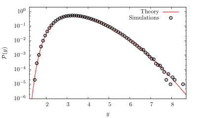
Figure 10: The distribution of $y=\int_{0}^{2}dt\ 1/x(t)$, where $x(t)$ is a Brownian excursion of length 2. The red full line is the analytical result and black symbols correspond to simulations.

Appendix C Laplace transform of $\mathcal{P}^{{(g_{s})}}\left(g_{s},h\right)$

In this final appendix, we take yet another route in the calculation of $\mathcal{P}^{{(g_{s})}}\left(g_{s},h\right)$ by finding its Laplace transform. The key point in this approach is to approximate the embedded random walk of the process by standard Brownian motion. Therefore, we expect our approximation to hold as long as $T\gg 1$. The approach is very similar in spirit to that of Appendix LABEL:sec:limiting_dist, but both Appendices are self-contained and can be read independently.

Let $x(t)$ denote the trajectory of a Brownian particle starting at $x(0)=x_{0}$, and $t_{f}$ its first passage time to 0. Then we argue that, in the Brownian motion picture, the original observable of interest of the process $g_{s}$ corresponds to the quantity $\mathcal{G}_{h}$,

$$\mathcal{G}_{h}=\int_{0}^{t_{f}}dtU_{h}(x(t)),$$ (67)

with $U_{h}(x)=1/(x+h)$. Effectively, the underlying exponential random variables $\xi(x(t))$ are replaced by their average. Such an approximation, which can be seen as a self-averaging property of the process, is well-justified because (i) the Brownian particle visits any state infinitely many times, and (ii) the exponential distribution has finite moments of any order. We are hence left with computing the distribution of the integral of a function $U_{h}(x)$ along a Brownian trajectory starting at $x(0)=x_{0}$ and ending at $x(t_{f})=0$. As usual, the problem is most conveniently solved by taking the Laplace transform of $\mathcal{G}_{h}$ (see the excellent review by Majumdar, Majumdar and Comtet (2005)). In particular, the Laplace transform of $\mathcal{P}\left(\mathcal{G}_{h}\right)$, which we denote by $\hat{\mathcal{P}}(u;h,x_{0})$, fulfills the following differential equation:

$$\frac{1}{2}\frac{\partial^{2}}{\partial x_{0}^{2}}\hat{\mathcal{P}}(u;h,x_{0})-u\ U_{h}(x_{0})\ \hat{\mathcal{P}}(u;h,x_{0})=0$$ (68)

with boundary conditions $\lim_{x_{0}\to\infty}\hat{\mathcal{P}}(u;h,x_{0})=0$ and $\lim_{x_{0}\to 0}\hat{\mathcal{P}}(u;h,x_{0})=1$. Note that this is a differential equation with respect to the initial position $x_{0}$. The general solution to this differential equation is given by

$$\sqrt{2}C_{1}\sqrt{u(h+x_{0})}I_{1}\left(2\sqrt{2}\sqrt{u(h+x_{0})}\right)-\sqrt{2}C_{2}\sqrt{u(h+x_{0})}K_{1}\left(2\sqrt{2}\sqrt{u(h+x_{0})}\right)$$ (69)

where $I_{1}(x)$ and $K_{1}(x)$ are modified Bessel functions of the first and second kind respectively, and $C_{1}$ and $C_{2}$ are constants to be determined via the boundary conditions. Because $I_{1}(x_{0})$ diverges for $x_{0}\to\infty$, $C_{1}$ must be zero, and $C_{2}$ is then fixed via the other boundary condition. Finally, by setting $x_{0}=1$ we reach a remarkably simple expression for the Laplace transform of $\mathcal{P}^{{(g_{s})}}\left(g_{s},h\right)$,

$$\hat{\mathcal{P}}(u;h)=\frac{\sqrt{u(h+1)}\ K_{1}\left(2\sqrt{2}\sqrt{u(h+1)}\right)}{\sqrt{uh}\ K_{1}\left(2\sqrt{2}\sqrt{uh}\right)}$$ (70)

This result is not only of interest in itself, but also provides a convenient way of evaluating $\mathcal{P}^{{(g_{s})}}\left(g_{s},h\right)$ by numerically inverting Eq. (70) (see Fig. 7 in the main text). We can also recover the asymptotic exponents $\gamma_{1},\gamma_{2}$ of $\mathcal{P}^{{(g_{s})}}\left(g_{s},h\right)$ directly from its Laplace transform, Eq. (70). To see this, we consider the first and second derivatives of $\hat{\mathcal{P}}(u;h)$,

$$-\partial_{u}\hat{\mathcal{P}}(u;h) \sim\sqrt{2/(hu)} \text{ for }1 \ll h$$ (71)

$$\partial_{uu}\hat{\mathcal{P}}(u;h) \sim\frac{2}{u} \text{ for }u \ll 1.$$ (72)

The first equation assumes large $h$, while the second does not; this allows us to recover the two scaling regions mentioned in the main text. Then it is easy to check that an application of a Tauberian theorem (Widder, 1946, p. 192) leads to Eq. (17b) and Eq. (17c) in the main text, recovering not only the asymptotic exponents $\gamma_{1},\gamma_{2}$, but also their associated first order amplitudes.

References

• Schorlemmer and Woessner (2008) D. Schorlemmer and J. Woessner, Bulletin of the Seismological Society of America 98, 2103 (2008).
• Lovejoy et al. (2003) S. Lovejoy, M. Lilley, N. Desaulniers-Soucy, and D. Schertzer, Physical Review E 68, 025301 (2003).
• Paczuski et al. (2005) M. Paczuski, S. Boettcher, and M. Baiesi, Phys. Rev. Lett. 95, 181102 (2005).
• Bak and Sneppen (1993) P. Bak and K. Sneppen, Phys. Rev. Lett. 71, 4083 (1993).
• Pruessner (2012) G. Pruessner, Self-Organised Criticality (Cambridge University Press, Cambridge, UK, 2012).
• Paczuski et al. (1996) M. Paczuski, S. Maslov, and P. Bak, Phys. Rev. E 53, 414 (1996), eprint arXiv:adap-org/9510002.
• Sneppen (1995) K. Sneppen, in Scale Invariance, Interfaces, and Non-Equilibrium Dynamics, edited by A. McKane, M. Droz, J. Vannimenus, and D. Wolf (Plenum Press, New York, NY, USA, 1995), pp. 295–302, NATO Advanced Study Institute on Scale Invariance, Interfaces, and Non-Equilibrium Dynamics, Cambridge, UK, Jun 20–30, 1994.
• Grassberger (1995) P. Grassberger, Phys. Lett. A 200, 277 (1995).
• Garber et al. (2009) A. Garber, S. Hallerberg, and H. Kantz, Phys. Rev. E 80, 026124 (2009).
• Gardiner (1997) C. W. Gardiner, Handbook of Stochastic Methods (Springer-Verlag, Berlin, Germany, 1997), 2nd ed.
• Hinrichsen (2000) H. Hinrichsen, Adv. Phys. 49, 815 (2000), eprint arXiv:cond-mat/0001070v2.
• Harris (1963) T. E. Harris, The Theory of Branching Processes (Springer-Verlag, Berlin, Germany, 1963).
• Peters et al. (2002) O. Peters, C. Hertlein, and K. Christensen, Phys. Rev. Lett. 88, 018701 (pages 4) (2002), eprint arXiv:cond-mat/0201468.
• Galassi et al. (2009) M. Galassi, J. Davies, J. Theiler, B. Gough, G. Jungman, P. Alken, M. Booth, and F. Rossi, GNU Scientific Library Reference Manual (Network Theory Ltd., 2009), 3rd ed., http://www.network-theory.co.uk/gsl/manual/, accessed 18 Aug 2009.
• Deluca and Corral (2013) A. Deluca and A. Corral, Acta Geophys. 61 (2013).
• Rubin et al. (2014) K. J. Rubin, G. Pruessner, and G. A. Pavliotis, J. Phys. A 47, 195001 (2014), eprint arXiv:1401.0695.
• Majumdar and Comtet (2004) S. N. Majumdar and A. Comtet, Phys. Rev. Lett. 92, 225501 (pages 4) (2004).
• Majumdar and Comtet (2005) S. N. Majumdar and A. Comtet, J. Stat. Phys. 119, 777 (2005).
• Mohanty (1979) G. Mohanty, Lattice path counting and applications (Academic Press New York, 1979).
• Christensen et al. (2008) K. Christensen, N. Farid, G. Pruessner, and M. Stapleton, Eur. Phys. J. B 62, 331 (2008).
• Corral (2009) A. Corral, J. Stat. Mech. P01022 (2009).
• Laurson et al. (2009) L. Laurson, X. Illa, and M. J. Alava, Journal of Statistical Mechanics: Theory and Experiment 2009, P01019 (2009), eprint arXiv:0810.0948.
• Knuth (1997) D. E. Knuth, Fundamental Algorithms, vol. 1 of The Art of Computer Programming (Addison-Wesley, Reading, MA, USA, 1997), 3rd ed.
• Stanley (1999) R. P. Stanley, Enumerative Combinatorics, Volume II, no. 62 in Cambridge Studies in Advanced Mathematics (Cambridge University Press, Cambridge, UK, 1999).
• Wolfram Research Inc. (2011) Wolfram Research Inc., Mathematica (Wolfram Research, Inc., Champaign, IL, USA, 2011), version 8.0.1.0.
• Abramowitz and Stegun (1970) M. Abramowitz and I. A. Stegun, eds., Handbook of Mathematical Functions (Dover Publications, Inc., New York, NY, USA, 1970).
• Chaichian and Demichev (2001) M. Chaichian and A. Demichev, Path Integrals in Physics: Volume I Stochastic Processes and Quantum Mechanics, Institute of physics series in mathematical and computational physics (Taylor & Francis, 2001), ISBN 9780750308014.
• Widder (1946) D. V. Widder, The Laplace Transform (Princeton University Press, Princeton, 1946).