Optimization Modulo Theories with Linear Rational Costs

Abstract

In the contexts of automated reasoning (AR) and formal verification (FV), important decision problems are effectively encoded into Satisfiability Modulo Theories (SMT). In the last decade efficient SMT solvers have been developed for several theories of practical interest (e.g., linear arithmetic, arrays, bit-vectors). Surprisingly, little work has been done to extend SMT to deal with optimization problems; in particular, we are not aware of any previous work on SMT solvers able to produce solutions which minimize cost functions over arithmetical variables. This is unfortunate, since some problems of interest require this functionality.

In the work described in this paper we start filling this gap. We present and discuss two general procedures for leveraging SMT to handle the minimization of linear rational cost functions, combining SMT with standard minimization techniques. We have implemented the procedures within the MathSAT SMT solver. Due to the absence of competitors in the AR, FV and SMT domains, we have experimentally evaluated our implementation against state-of-the-art tools for the domain of linear generalized disjunctive programming (LGDP), which is closest in spirit to our domain, on sets of problems which have been previously proposed as benchmarks for the latter tools. The results show that our tool is very competitive with, and often outperforms, these tools on these problems, clearly demonstrating the potential of the approach.

Authors’ addresses: Roberto Sebastiani (roberto.sebastiani@unitn.it), Silvia Tomasi (silvia.tomasi@disi.unitn.it), DISI, Università di Trento, via Sommarive 9, I-38123 Povo, Trento, Italy. Roberto Sebastiani is supported by Semiconductor Research Corporation (SRC) under GRC Research Project 2012-TJ-2266 WOLF.

1 Introduction

In the contexts of automated reasoning (AR) and formal verification (FV), important decision problems are effectively encoded into and solved as Satisfiability Modulo Theories (SMT) problems. In the last decade efficient SMT solvers have been developed, that combine the power of modern conflict-driven clause-learning (CDCL) SAT solvers with dedicated decision procedures ($\mathcal{T}$-$\mathsf{Solvers}$) for several first-order theories of practical interest like, e.g., those of equality with uninterpreted functions ($\mathcal{EUF}$), of linear arithmetic over the rationals ($\mathcal{LA}(\mathbb{Q})$) or the integers ($\mathcal{LA}(\mathbb{Z})$), of arrays ($\mathcal{AR}$), of bit-vectors ($\mathcal{BV}$), and their combinations. We refer the reader to [Sebastiani (2007), Barrett et al. (2009)] for an overview.

Many SMT-encodable problems of interest, however, may require also the capability of finding models that are optimal wrt. some cost function over continuous arithmetical variables. For example, in (SMT-based) planning with resources [Wolfman and Weld (1999)] a plan for achieving a certain goal must be found which not only fulfills some resource constraints (e.g. on time, gasoline consumption, among others) but that also minimizes the usage of some of such resources; in SMT-based model checking with timed or hybrid systems (e.g. [Audemard et al. (2002), Audemard et al. (2005)]) you may want to find executions which minimize some parameter (e.g. elapsed time), or which minimize/maximize the value of some constant parameter (e.g., a clock timeout value) while fulfilling/violating some property (e.g., minimize the closure time interval of a rail-crossing while preserving safety). This also involves, as particular subcases, problems which are traditionally addressed as linear disjunctive programming (LDP) [Balas (1998)] or linear generalized disjunctive programming (LGDP) [Raman and Grossmann (1994), Sawaya and Grossmann (2012)], or as SAT/SMT with Pseudo-Boolean (PB) constraints and (weighted partial) MaxSAT/SMT problems [Roussel and Manquinho (2009), Li and Manyà (2009), Nieuwenhuis and Oliveras (2006), Cimatti et al. (2010), Cimatti et al. (2013a)]. Notice that the two latter problems can be encoded into each other.

Surprisingly, little work has been done so far to extend SMT to deal with optimization problems [Nieuwenhuis and Oliveras (2006), Cimatti et al. (2010), Sebastiani and Tomasi (2012), Dillig et al. (2012), Cimatti et al. (2013a), Manolios and Papavasileiou (2013)] (see §6). In particular, to the best of our knowledge, most such works aim at minimizing cost functions over Boolean variables (i.e., SMT with PB cost functions or MaxSMT), whilst we are not aware of any previous work on SMT solvers able to produce solutions which minimize cost functions over arithmetical variables. Notice that the former can be encoded into the latter, but not vice versa.

In this this work we start filling this gap. We present two general procedures for adding to SMT the functionality of finding models which minimize some $\mathcal{LA}(\mathbb{Q})$ cost variable —$\mathcal{T}$ being some possibly-empty stably-infinite theory s.t. $\mathcal{T}$ and $\mathcal{LA}(\mathbb{Q})$ are signature disjoint. These two procedures combine standard SMT and minimization techniques: the first, called offline, is much simpler to implement, since it uses an incremental SMT solver as a black-box, whilst the second, called inline, is more sophisticate and efficient, but it requires modifying the code of the SMT solver. This distinction is important, since the source code of many SMT solvers is not publicly available.

We have implemented these procedures within the MathSAT5 SMT solver [Cimatti et al. (2013b)]. Due to the absence of competitors from AR, FV and SMT domains (§6), we have experimentally evaluated our implementation against state-of-the-art tools for the domain of LGDP, which is closest in spirit to our domain, on sets of problems which have been previously proposed as benchmarks for the latter tools, and on other problem sets. (Notice that LGDP is limited to plain $\mathcal{LA}(\mathbb{Q})$, so that, e.g., it cannot handle combinations of theories like $\mathcal{LA}(\mathbb{Q})\cup\mathcal{T}$.) The results show that our tool is very competitive with, and often outperforms, these tools on these problems, clearly demonstrating the potential of the approach.

Content. The rest of the paper is organized as follows: in §2 we provide some background knowledge about SAT, SMT, and LGDP; in §3 we formally define the problem addressed, provide the necessary formal results for its solution, and show how the problem generalizes many known optimization problems; in §4 we present our novel procedures; in §5 we present an extensive experimental evaluation; in §6 we survey the related work; in §7 we briefly conclude and highlight directions for future work. In Appendix A we provide the proofs of all the theorems presented in the paper.

Disclaimer. This work was presented in a preliminary form in a much shorter paper at IJCAR 2012 conference [Sebastiani and Tomasi (2012)]. Here the content is extended in many ways: first, we provide the theoretical foundations of the procedures, including formal definitions, theorems and relative proofs; second, we provide a much more detailed description and analysis of the procedures, describing in details issues which were only hinted in the conference paper; third, we introduce novel improvements to the procedures; fourth, we provide a much more extended empirical evaluation; finally, we provide a detailed description of the background and of the related work.

2 Background

In this section we provide the necessary background about SAT (§2.1), SMT (§2.2), and LGDP (§2.3). We assume a basic background knowledge about logic and operational research. We provide a uniform notation for SAT and SMT: we use boldface lowcase letters ${{\bf a}},{{\bf y}}$ for arrays and boldface upcase letters ${{\bf A}},{{\bf Y}}$ for matrices (i.e., two-dimensional arrays), standard lowcase letters a, y for single rational variables/constants or indices and standard upcase letters ${A}$, ${Y}$ for Boolean atoms and index sets; we use the first five letters in the various forms ${{\bf a}},...{{\bf e}}$, … ${A},...{E}$, to denote constant values, the last five ${{\bf v}},...{{\bf z}}$, $...$ ${V},...{Z}$ to denote variables, and the letters ${i},{j},{k},{I},{J},{K}$ for indexes and index sets respectively, subscripts $._{j}$ denote the $j$-th element of an array or matrix, whilst superscripts $.^{ij}$ are just indexes, being part of the name of the element. We use lowcase Greek letters $\varphi,\phi,\psi,\mu,\eta$ for denoting formulas and upcase ones $\Phi,\Psi$ for denoting sets of formulas.

Remark 2.1.

Although we refer to quantifier-free formulas, as it is standard practice in SAT, SMT, CSP and OR communities, with a little abuse of terminology we call “Boolean variables” the propositional atoms and we call “variables” the free constants $x_{i}$ in quantifier-free $\mathcal{LA}(\mathbb{Q})$-atoms like “$(3x_{1}-2x_{2}+x_{3}\leq 3)$”.

We assume the standard syntactic and semantic notions of propositional logic. Given a non-empty set of primitive propositions $\mathcal{P}=\{p_{1},p_{2},\ldots\}$, the language of propositional logic is the least set of formulas containing $\mathcal{P}$ and the primitive constants $\top$ and $\bot$ (“true” and “false”) and closed under the set of standard propositional connectives $\{\neg,\wedge,\vee,\rightarrow,\leftrightarrow\}$. We call a propositional atom every primitive proposition in $\mathcal{P}$, and a propositional literal every propositional atom (positive literal) or its negation (negative literal). We implicitly remove double negations: e.g., if $l$ is the negative literal $\neg p_{i}$, then by $\neg l$ we mean $p_{i}$ rather than $\neg\neg p_{i}$. With a little abuse of notation, we represent a truth assignment $\mu$ indifferently either as a set of literals $\{l_{i}\}_{i}$, with the intended meaning that a positive [resp. negative] literal $p_{i}$ means that $p_{i}$ is assigned to true [resp. false], or as a conjunction of literals $\bigwedge_{i}l_{i}$; thus, e.g., we may say “$l_{i}\in\mu$” or “$\mu_{1}\subseteq\mu_{2}$”, but also “$\neg\mu$” meaning the clause “$\bigvee_{i}\neg l_{i}$”.

A propositional formula is in conjunctive normal form, CNF, if it is written as a conjunction of disjunctions of literals: $\bigwedge_{i}\bigvee_{j}l_{ij}$. Each disjunction of literals $\bigvee_{j}l_{ij}$ is called a clause. A unit clause is a clause with only one literal.

The above notation and terminology about [positive/negative] literals, truth assignments, CNF and [unit] clauses extend straightforwardly to quantifier-free first-order formulas.

2.1 SAT and CDCL SAT solvers

We present here a brief description on how a Conflict-Driven Clause-Learning (CDCL) SAT solver works. We refer the reader, e.g., to [Marques-Silva and Sakallah (1996), Moskewicz et al. (2001), Marques-Silva et al. (2009)] for a detailed description.

We assume the input propositional formula $\varphi$ is in CNF. (If not, it is first CNF-ized as in [Plaisted and Greenbaum (1986)].) The assignment $\mu$ is initially empty, and it is updated in a stack-based manner. The SAT solver performs an external loop, alternating three main phases: Decision, Boolean Constraint Propagation (BCP) and Backjumping and Learning.

During Decision an unassigned literal $l$ from $\varphi$ is selected according to some heuristic criterion, and it is pushed into $\mu$. $l$ is called decision literal and the number of decision literals which are contained in $\mu$ immediately after deciding $l$ is called the decision level of $l$.

Then BCP iteratively deduces the literals $l_{1},l_{2},...$ deriving from the current assignment and pushes them into $\mu$. BCP is based on the iterative application of unit propagation: if all but one literals in a clause are false, then the only unassigned literal $l$ is added to $\mu$, all negative occurrences of $l$ in other clauses are declared false and all clauses with positive occurrences of $l$ are declared satisfied. Current SAT solvers include rocket-fast implementations of BCP based on the two-watched-literal scheme, see [Moskewicz et al. (2001), Marques-Silva et al. (2009)]. BCP is repeated until either no more literals can be deduced, so that the loop goes back to another decision step, or no more Boolean variable can be assigned, so that the SAT solver ends returning sat, or $\mu$ falsifies some clause $\psi$ of $\varphi$ (conflicting clause).

In the latter case, Backjumping and Learning are performed. A process of conflict analysis  detects a subset $\eta$ of $\mu$ which actually caused the falsification of $\psi$ (conflict set)  and the decision level $\sf{blevel}$ where to backtrack. Additionally, the conflict clause $\psi^{\prime}\stackrel{{\scriptstyle\text{\tiny def}}}{{=}}\neg\eta$ is added to $\varphi$ (Learning) and the procedure backtracks up to $\sf{blevel}$ (Backjumping), popping out of $\mu$ all literals whose decision level is greater than $\sf{blevel}$. When two contradictory literals $l,\neg l$ are assigned at level 0, the loop terminates, returning unsat.

Notice that CDCL SAT solvers implement “safe” strategies for deleting clauses when no more necessary, which guarantee the use of polynomial space without affecting the termination, correctness and completeness of the procedure. (See e.g. [Marques-Silva et al. (2009), Nieuwenhuis et al. (2006)].)

Many modern CDCL SAT solvers provide a stack-based incremental interface (see e.g. [Eén and Sörensson (2004)]), by which it is possible to push/pop sub-formulas $\phi_{i}$ into a stack of formulas $\Phi\stackrel{{\scriptstyle\text{\tiny def}}}{{=}}\{{\phi_{1},...,\phi_{k}}\}$, and check incrementally the satisfiability of $\bigwedge_{i=1}^{k}\phi_{i}$. The interface maintains most of the information about the status of the search from one call to the other, in particular it records the learned clauses (plus other information). Consequently, when invoked on $\Phi$ the solver can reuse a clause $\psi$ which was learned during a previous call on some $\Phi^{\prime}$ if $\psi$ was derived only from clauses which are still in $\Phi$ —provided $\psi$ was not discharged in the meantime; in particular, if $\Phi^{\prime}\subseteq\Phi$, then the solver can reuse all clauses learned while solving $\Phi^{\prime}$.

Another important feature of many incremental CDCL SAT solvers is their capability, when $\Phi$ is found unsatisfiable, to return a subset of formulas in $\Phi$ which caused the unsatisfiability of $\Phi$. This is related to the problem of finding an unsatisfiable core of a formula, see e.g. [Lynce and Marques-Silva (2004)]. Notice that such subset is not unique, and it is not necessarily minimal.

2.2 SMT and Lazy SMT solvers

We assume a basic background knowledge on first-order logic. to ground formulas/literals/atoms in the language of $\mathcal{T}$ ($\mathcal{T}$-formulas/literals/atoms hereafter). Notice that, for better readability, with a little abuse of notation we often refer to a theory $\mathcal{T}$ instead of its corresponding signature; also by “empty theory” we mean the empty theory over the empty signature; finally, by adopting the terminology in Remark 2.1, we say that a variable belongs to the signature of a theory $\mathcal{T}$ (or simply that it belongs to a theory $\mathcal{T}$).

A theory solver for $\mathcal{T}$, $\mathcal{T}$-$\mathsf{Solver}$, is a procedure able to decide the $\mathcal{T}$-satisfiability of a conjunction/set $\mu$ of $\mathcal{T}$-literals. If $\mu$ is $\mathcal{T}$-unsatisfiable, then $\mathcal{T}$-$\mathsf{Solver}$ returns unsat and a set/conjunction $\eta$ of $\mathcal{T}$-literals in $\mu$ which was found $\mathcal{T}$-unsatisfiable; $\eta$ is called a $\mathcal{T}$-conflict set, and $\neg\eta$ a $\mathcal{T}$-conflict clause. If $\mu$ is $\mathcal{T}$-satisfiable, then $\mathcal{T}$-$\mathsf{Solver}$ returns sat; it may also be able to return some unassigned $\mathcal{T}$-literal $l\not\in\mu$ from a set of all available $\mathcal{T}$-literals, s.t. $\{l_{1},...,l_{n}\}\models_{\mathcal{T}}l$, where $\{l_{1},...,l_{n}\}\subseteq\mu$. We call this process $\mathcal{T}$-deduction and $(\bigvee_{i=1}^{n}\neg l_{i}\vee l)$ a $\mathcal{T}$-deduction clause. Notice that $\mathcal{T}$-conflict and $\mathcal{T}$-deduction clauses are valid in $\mathcal{T}$. We call them $\mathcal{T}$-lemmas.

Given a $\mathcal{T}$-formula $\varphi$, the formula $\varphi^{p}$ obtained by rewriting each $\mathcal{T}$-atom in $\varphi$ into a fresh atomic proposition is the Boolean abstraction of $\varphi$, and $\varphi$ is the refinement of $\varphi^{p}$. Notationally, we indicate by $\varphi^{p}$ and $\mu^{p}$ the Boolean abstraction of $\varphi$ and $\mu$, and by $\varphi$ and $\mu$ the refinements of $\varphi^{p}$ and $\mu^{p}$ respectively. With a little abuse of notation, we say that $\mu^{p}$ is $\mathcal{T}$-(un)satisfiable iff $\mu$ is $\mathcal{T}$-(un)satisfiable. We say that the truth assignment $\mu$ propositionally satisfies the formula $\varphi$, written $\mu\models_{p}\varphi$, if $\mu^{p}\models\varphi^{p}$.

In a lazy $\text{SMT}(\mathcal{T})$ solver, the Boolean abstraction $\varphi^{p}$ of the input formula $\varphi$ is given as input to a CDCL SAT solver, and whenever a satisfying assignment $\mu^{p}$ is found s.t. $\mu^{p}\models\varphi^{p}$, the corresponding set of $\mathcal{T}$-literals $\mu$ is fed to the $\mathcal{T}$-$\mathsf{Solver}$; if $\mu$ is found $\mathcal{T}$-consistent, then $\varphi$ is $\mathcal{T}$-consistent; otherwise, $\mathcal{T}$-$\mathsf{Solver}$ returns a $\mathcal{T}$-conflict set $\eta$ causing the inconsistency, so that the clause $\neg\eta^{p}$ is used to drive the backjumping and learning mechanism of the SAT solver. The process proceeds until either a $\mathcal{T}$-consistent assignment $\mu$ is found, or no more assignments are available ($\varphi$ is $\mathcal{T}$-inconsistent).

Important optimizations are early pruning and $\mathcal{T}$-propagation. The $\mathcal{T}$-$\mathsf{Solver}$ is invoked also when an assignment $\mu$ is still under construction: if it is $\mathcal{T}$-unsatisfiable, then the procedure backtracks, without exploring the (possibly many) extensions of $\mu$; if not, and if the $\mathcal{T}$-$\mathsf{Solver}$ is able to perform a $\mathcal{T}$-deduction $\{l_{1},...,l_{n}\}\models_{\mathcal{T}}l$, then $l$ can be unit-propagated, and the $\mathcal{T}$-deduction clause $(\bigvee_{i=1}^{n}\neg l_{i}\vee l)$ can be used in backjumping and learning. To this extent, in order to maximize the efficiency, most $\mathcal{T}$-solvers are incremental and backtrackable, that is, they are called via a push&pop interface, maintaining and reusing the status of the search from one call and the other.

Another optimization is pure-literal filtering: if some $\mathcal{LA}(\mathbb{Q})$-atoms occur only positively [resp. negatively] in the original formula (learned clauses are ignored), then we can safely drop every negative [resp. positive] occurrence of them from the assignment $\mu$ to be checked by the $\mathcal{T}$-$\mathsf{Solver}$ [Sebastiani (2007)]. Intuitively, since such occurrences play no role in satisfying the formula, the resulting partial assignment ${\mu^{p}}^{\prime}$ still satisfies $\varphi^{p}$. The benefits of this action are twofold: (i) it reduces the workload for the $\mathcal{T}$-$\mathsf{Solver}$ by feeding to it smaller sets; (ii) it increases the chance of finding a $\mathcal{T}$-consistent satisfying assignment by removing “useless” $\mathcal{T}$-literals which may cause the $\mathcal{T}$-inconsistency of $\mu$.

The above schema is a coarse abstraction of the procedures underlying all the state-of-the-art lazy SMT tools. The interested reader is pointed to, e.g., [Nieuwenhuis et al. (2006), Sebastiani (2007), Barrett et al. (2009)] for details and further references. Importantly, some SMT solvers, including MathSAT, inherit from their embedded SAT solver the capabilities of working incrementally and of returning the subset of input formulas causing the inconsistency, as described in §2.1.

The Theory of Linear Arithmetic on the rationals ($\mathcal{LA}(\mathbb{Q})$) and on the integers ($\mathcal{LA}(\mathbb{Z})$) is one of the theories of main interest in SMT. It is a first-order theory whose atoms are of the form $(a_{1}x_{1}+\ldots+a_{n}x_{n}\diamond b)$, i.e. $({{\bf a}}{{\bf x}}\diamond b)$, s.t $\diamond\in\{{=,\neq,<,>,\leq,\geq}\}$.

Efficient incremental and backtrackable procedures have been conceived in order to decide $\mathcal{LA}(\mathbb{Q})$ [Dutertre and de Moura (2006)] and $\mathcal{LA}(\mathbb{Z})$ [Griggio (2012)]. In particular, for $\mathcal{LA}(\mathbb{Q})$ most SMT solvers implement variants of the simplex-based algorithm by Dutertre and de Moura [Dutertre and de Moura (2006)] which is specifically designed for integration in a lazy SMT solver, since it is fully incremental and backtrackable and allows for aggressive $\mathcal{T}$-deduction. Another benefit of such algorithm is that it handles strict inequalities directly. Its method is based on the fact that a set of $\mathcal{LA}(\mathbb{Q})$ atoms $\Gamma$ containing strict inequalities $S=\{0<t_{1},\ldots,0<t_{n}\}$ is satisfiable iff there exists a rational number $\epsilon>0$ such that $\Gamma_{\epsilon}\stackrel{{\scriptstyle\text{\tiny def}}}{{=}}(\Gamma\cup S_{\epsilon})\setminus S$ is satisfiable, s.t. $S_{\epsilon}\stackrel{{\scriptstyle\text{\tiny def}}}{{=}}\{\epsilon\leq t_{1},\ldots,\epsilon\leq t_{n}\}$. The idea of [Dutertre and de Moura (2006)] is that of treating the infinitesimal parameter $\epsilon$ symbolically instead of explicitly computing its value. Strict bounds $(x<b)$ are replaced with weak ones $(x\leq b-\epsilon)$, and the operations on bounds are adjusted to take $\epsilon$ into account. We refer the reader to [Dutertre and de Moura (2006)] for details.

2.3 Linear Generalized Disjunctive Programming

Mixed Integer Linear Programming (MILP) is an extension of Linear Programming (LP) involving both discrete and continuous variables [Lodi (2009)]. MILP problems have the following form:

$$\min\{{{\bf c}}{{\bf x}}:{{\bf A}}{{\bf x}}\geq{{\bf b}},{{\bf x}}\geq 0,{{\bf x}}_{j}\in\mathbb{Z}\mbox{ }\forall j\in I\}$$ (1)

where ${{\bf A}}$ is a matrix, ${{\bf c}}$ and ${{\bf b}}$ are constant vectors and ${{\bf x}}$ the variable vector. A large variety of techniques and tools for MILP are available, mostly based on efficient combinations of LP, branch-and-bound search mechanism and cutting-plane methods, resulting in a branch-and-cut approach (see e.g. [Lodi (2009)]). SAT techniques have also been incorporated into these procedures for MILP (see [Achterberg et al. (2008)]).

The branch-and-bound search iteratively partitions the solution space of the original MILP problem into subproblems and solves their LP relaxation (i.e. a MILP problem where the integrality constraint on the variables ${{\bf x}}_{j}$, for all $j\in I$, is dropped) until all variables are integral in the optimal solution of the LP relaxation. Cutting planes (e.g. Gomory mixed-integer and lift-and-project cuts [Lodi (2009)]) are linear inequalities that can be inferred and added to the original MILP problem and its subproblems in order to cut away non-integer solutions of the LP relaxation and obtain tighter relaxations.

Linear Disjunctive Programming (LDP) problems are LP problems where linear constraints are connected by the logical operations of conjunction and disjunction (see, e.g., [Balas (1998)]). The constraint set can be expressed by a disjunction of linear systems (Disjunctive Normal Form):

$$\bigvee_{i\in I}({{\bf A}}^{i}{{\bf x}}\geq{{\bf b}}^{i})$$ (2)

or, alternatively, as a conjunction (Conjunctive Normal Form):

$$({{\bf A}}{{\bf x}}\geq{{\bf b}})\wedge\bigwedge_{j=1}^{t}\bigvee_{k\in I_{j}}({{\bf c}}^{k}{{\bf x}}\geq d^{k})$$ (3)

or in an intermediate form called Regular Form (see, e.g., [Balas (1983)]). Notice that (3) can be obtained from (2) by factoring out the common inequalities $({{\bf A}}{{\bf x}}\geq{{\bf b}})$ and then by applying the distributivity of $\wedge$ and $\vee$, although the latter step can cause a blowup in size. LDP problems are effectively solved by the lift-and-project approach which combines a family of cutting planes, called lift-and-project cuts, and the branch-and-bound schema (see, e.g., [Balas and Bonami (2007)]).

Linear Generalized Disjunctive Programming (LGDP), is a generalization of LDP which has been proposed in [Raman and Grossmann (1994)] as an alternative model to the MILP problem. Unlike MILP, which is based entirely on algebraic equations and inequalities, the LGDP model allows for combining algebraic and logical equations with Boolean propositions through Boolean operations, providing a much more natural representation of discrete decisions. Current approaches successfully address LGDP by reformulating and solving it as a MILP problem [Raman and Grossmann (1994), Vecchietti and Grossmann (2004), Sawaya and Grossmann (2005), Sawaya and Grossmann (2012)]; these reformulations focus on efficiently encoding disjunctions and logic propositions into MILP, so as to be fed to an efficient MILP solver like Cplex.

The general formulation of a LGDP problem is the following [Raman and Grossmann (1994)]:

min $$\sum_{k\in K}{{\bf z}}_{k}+{{\bf d}}{{\bf x}}$$

s.t. $${{\bf B}}{{\bf x}}\leq{{\bf b}}$$

$$\bigvee_{j\in J_{k}}\Biggr{[}\begin{array}[]{c}Y^{jk}\\ {{\bf A}}^{jk}{{\bf x}}\leq{{\bf a}}^{jk}\\ {{\bf z}}_{k}=c^{jk}\\ \end{array}\Biggr{]} \forall k\in K$$

$$\phi$$

$${{\bf 0}}\leq{{\bf x}}\leq{{\bf e}}$$

$${{\bf z}}_{k},c^{jk}\in\mathbb{R}_{+}^{1},Y^{jk}\in\{True,False\} \forall j\in J_{k},\forall k\in K$$

where ${{\bf x}}$ is a vector of positive rational variables, ${{\bf d}}$ is a vector of positive rational values representing the cost-per-unit of each variable in ${{\bf x}}$, ${{\bf z}}$ is a vector of positive rational variables representing the cost assigned to each disjunction, $c^{jk}$ are positive constant values, ${{\bf e}}$ is a vector of upper bounds for ${{\bf x}}$ and $Y^{jk}$ are Boolean variables.

The disequalities ${{\bf B}}{{\bf x}}\leq{{\bf b}}$, where $({{\bf B}},{{\bf b}})$ is a $m\times(n+1)$ matrix, are the “common” constraints that must always hold.

Each disjunction $k\in K$ consists in at least two disjuncts $j\in J_{k}$, s.t. the ${jk}$-th disjunct contains:

• the Boolean variable $Y^{jk}$, representing discrete decisions,

• a set of linear constraints ${{\bf A}}^{jk}{{\bf x}}\leq{{\bf a}}^{jk}$, where $({{\bf A}}^{jk},{{\bf a}}^{jk})$ is a $m_{jk}\times(n+1)$ matrix,

• the equality ${{\bf z}}_{k}=c^{jk}$, assigning the value $c^{jk}$ to the cost variable ${{\bf z}}_{k}$.

Each disjunct is true if and only if all the three elements (i)-(iii) above are true. $\phi$ is a propositional formula, expressed in Conjunctive Normal Form, which must contain the “xor” constraints $\bigoplus_{j\in J_{k}}Y^{jk}$ for each $k\in K$, plus possibly other constraints. Intuitively, for each $k\in K$, the only variable $Y^{jk}$ which is set to true selects the set of disequalities ${{\bf A}}^{jk}{{\bf x}}\leq{{\bf a}}^{jk}$ which are enforced and hence it selects the relative cost $c^{jk}$ of this choice to be assigned to the cost variable ${{\bf z}}_{k}$.

LGDP problems can be solved using MILP solvers by reformulating the original problem in different ways; big-M (BM) and convex hull (CH) are the two most common reformulations. In BM, the Boolean variables $Y^{jk}$ and the logic constraints $\phi$ are replaced by binary variables ${{\bf Y}}_{jk}$ and linear inequalities as follows [Raman and Grossmann (1994)]:

min $$\sum_{k\in K}\sum_{j\in J_{k}}c^{jk}{{\bf Y}}_{jk}+{{\bf d}}{{\bf x}}$$

s.t. $${{\bf B}}{{\bf x}}\leq{{\bf b}}$$

$${{\bf A}}^{jk}{{\bf x}}-{{\bf a}}^{jk}\leq{{\bf M}}^{jk}(1-{{\bf Y}}_{jk}) \forall j\in J_{k},\forall k\in K$$

$$\sum_{j\in J_{k}}{{\bf Y}}_{jk}=1 \forall k\in K$$

$${{\bf D}}{{\bf Y}}\leq{{\bf D^{\prime}}}$$

$${{\bf x}}\in\mathbb{R}^{n}\ s.t.\ {{\bf 0}}\leq{{\bf x}}\leq{{\bf e}},{{\bf Y}}_{jk}\in\{0,1\} \forall j\in J_{k},\forall k\in K$$

where ${{\bf M}}^{jk}$ are the ‘”big-M“ parameters that makes redundant the system of constraint $j\in J_{k}$ in the disjunction $k\in K$ when ${{\bf Y}}_{jk}=0$ and the constraints ${{\bf D}}{{\bf Y}}\leq{{\bf D^{\prime}}}$ are derived from $\phi$.

In CH, the Boolean variables $Y^{jk}$ are replaced by binary variables ${{\bf Y}}_{jk}$ and the variables ${{\bf x}}\in\mathbb{R}^{n}$ are disaggregated into new variables ${{\bf v}}\in\mathbb{R}^{n}$ in the following way:

min $$\sum_{k\in K}\sum_{j\in J_{k}}c^{jk}{{\bf Y}}_{jk}+{{\bf d}}{{\bf x}}$$

s.t. $${{\bf B}}{{\bf x}}\leq{{\bf b}}$$

$${{\bf A}}^{kj}{{\bf v}}^{jk}\leq{{\bf a}}^{jk}{{\bf Y}}_{jk} \forall j\in J_{k},\forall k\in K$$

$${{\bf x}}=\sum_{j\in J_{k}}{{\bf v}}_{jk} \forall k\in K$$

$${{\bf v}}_{jk}\leq{{\bf Y}}_{jk}{{\bf e}}^{jk} \forall j\in J_{k},\forall k\in K$$

$$\sum_{j\in J_{k}}{{\bf Y}}_{jk}=1 \forall k\in K$$

$${{\bf D}}{{\bf Y}}\leq{{\bf D^{\prime}}}$$

$${{\bf x}},{{\bf v}}\in\mathbb{R}^{n}\ s.t.\ {{\bf 0}}\leq{{\bf x}},{{\bf v}},\ {{\bf Y}}_{jk}\in\{0,1\} \forall j\in J_{k},\forall k\in K$$

where constant ${{\bf e}}^{jk}$ are upper bounds for variables ${{\bf v}}$ chosen to match the upper bounds on the variables ${{\bf x}}$.

Sawaya and Grossman [Sawaya and Grossmann (2005)] observed two facts. First, the relaxation of BM is often weak causing a higher number of nodes examined in the branch-and-bound search. Second, the disaggregated variables and new constraints increase the size of the reformulation leading to a high computational effort. In order to overcome these issues, they proposed a cutting plane method that consists in solving a sequence of BM relaxations with cutting planes that are obtained from CH relaxations. They provided an evaluation of the presented algorithm on three different problems: strip-packing, retrofit planning and zero-wait job-shop scheduling problems.

3 Optimization in $\text{SMT}(\mathcal{LA}(\mathbb{Q})\cup\mathcal{T})$

In this section we define the problem addressed (§3.1), we introduce the formal foundations for its solution (§3.2), and we show how it generalizes many known optimization problems from the literature (§3.3).

3.1 Basic Definitions and Notation

In this paper we consider only signature-disjoint stably-infinite theories with equality $\mathcal{T}_{i}$ (“Nelson-Oppen theories” [Nelson and Oppen (1979)]) and we focus our interest on $\mathcal{LA}(\mathbb{Q})$. In particular, in what follows we assume $\mathcal{T}$ to be some stably-infinite theory with equality, s.t. $\mathcal{LA}(\mathbb{Q})$ and $\mathcal{T}$ are signature-disjoint. $\mathcal{T}$ can also be a combination of Nelson-Oppen theories.

We assume the standard model of $\mathcal{LA}(\mathbb{Q})$, whose domain is the set of rational numbers $\mathbb{Q}$.

Definition 3.1 ($\text{OMT}(\mathcal{LA}(\mathbb{Q})\cup\mathcal{T})$, $\text{OMT}(\mathcal{LA}(\mathbb{Q}))$, and $\mathsf{min}_{\sf cost}$.).

Let $\varphi$ be a ground $\text{SMT}(\mathcal{LA}(\mathbb{Q})\cup\mathcal{T})$ formula, and ${\sf cost}$ be a $\mathcal{LA}(\mathbb{Q})$ variable occurring in $\varphi$. We call an Optimization Modulo $\mathcal{LA}(\mathbb{Q})\cup\mathcal{T}$ problem, written $\text{OMT}(\mathcal{LA}(\mathbb{Q})\cup\mathcal{T})$, the problem of finding a model for $\varphi$ (if any) whose value of ${\sf cost}$ is minimum. We denote such value as $\mathsf{min}_{\sf cost}(\varphi)$. If $\varphi$ is $\mathcal{LA}(\mathbb{Q})\cup\mathcal{T}$-unsatisfiable, then $\mathsf{min}_{\sf cost}(\varphi)$ is $+\infty$; if there is no minimum value for ${\sf cost}$, then $\mathsf{min}_{\sf cost}(\varphi)$ is $-\infty$. We call an Optimization Modulo $\mathcal{LA}(\mathbb{Q})$ problem, written $\text{OMT}(\mathcal{LA}(\mathbb{Q}))$, an $\text{OMT}(\mathcal{LA}(\mathbb{Q})\cup\mathcal{T})$ problem where $\mathcal{T}$ is the empty theory.

A dual definition where we look for a maximum value is easy to formulate.

In order to make the discussion simpler, we assume w.l.o.g. that all $\mathcal{LA}(\mathbb{Q})\cup\mathcal{T}$ formulas are pure [Nelson and Oppen (1979)]. With a little abuse of notation, we say that an atom in a ground $\mathcal{T}_{1}\cup\mathcal{T}_{2}$ formula is $\mathcal{T}_{i}$-pure if it contains only variables and symbols from the signature of $\mathcal{T}_{i}$, for every $i\in\{1,2\}$; a $\mathcal{T}_{1}\cup\mathcal{T}_{2}$ ground formula is pure iff all its atoms are either $\mathcal{T}_{1}$-pure or $\mathcal{T}_{2}$-pure. Although the purity assumption is not necessary (see [Barrett et al. (2002)]), it simplifies the explanation, since it allows us to speak about “$\mathcal{LA}(\mathbb{Q})$-atoms” or “$\mathcal{T}$-atoms” without further specifying. Moreover, every non-pure formula can be easily purified [Nelson and Oppen (1979)].

We also assume w.l.o.g. that all $\mathcal{LA}(\mathbb{Q})$-atoms containing the variable ${\sf cost}$ are in the form $(t\bowtie{\sf cost})$, s.t. $\bowtie\ \in\{{=,\leq,\geq,<,>}\}$ and ${\sf cost}$ does not occur in $t$.

Definition 3.2 (Bounds and range for ${\sf cost}$).

If $\varphi$ is in the form $\varphi^{\prime}\wedge({\sf cost}<c)$ [resp. $\varphi^{\prime}\wedge\neg({\sf cost}<c)$] for some value $c\in\mathbb{Q}$, then we call $c$ an upper bound [resp. lower bound] for ${\sf cost}$. If $\mathsf{ub}$ [resp $\mathsf{lb}$ ] is the minimum upper bound [resp. the maximum lower bound] for $\varphi$, we also call the interval $[\mathsf{lb},\mathsf{ub}[$ the range of ${\sf cost}$.

We adopt the convention of defining upper bounds to be strict and lower bounds to be non-strict for a practical reason: typically an upper bound $({\sf cost}<c)$ derives from the fact that a model $\mathcal{I}$ of cost $c$ has been previously found, whilst a lower bound $\neg({\sf cost}<c)$ derives either from the user’s knowledge (e.g. “the cost cannot be lower than zero”) of from the fact that the formula $\varphi\wedge({\sf cost}<c)$ has been previously found $\mathcal{T}$-unsatisfiable whilst $\varphi$ has not.

3.2 Theoretical Results

We present here the theoretical foundations of our procedures. The proofs of the novel results are reported in Appendix A.

The following facts follow straightforwardly from Definition 3.1.

Proposition 3.3.

Let $\varphi,\varphi_{1},\varphi_{2}$ be $\mathcal{LA}(\mathbb{Q})\cup\mathcal{T}$-formulas and $\mu_{1},\mu_{2}$ be truth assignments.

• If $\varphi_{1}\models\varphi_{2}$, then $\mathsf{min}_{\sf cost}(\varphi_{1})\geq\mathsf{min}_{\sf cost}(\varphi_{2})$.

• If $\mu_{1}\supseteq\mu_{2}$, then $\mathsf{min}_{\sf cost}(\mu_{1})\geq\mathsf{min}_{\sf cost}(\mu_{2})$.

• $\varphi$ is $\mathcal{LA}(\mathbb{Q})\cup\mathcal{T}$-satisfiable if and only if $\mathsf{min}_{\sf cost}(\varphi)<+\infty$.

We recall first some definitions and results from the literature.

Definition 3.4.

We say that a collection ${\cal M\/}:=\{\mu_{1},\ldots,\mu_{n}\}$ of (possibly partial) assignments propositionally satisfying $\varphi$ is complete iff, for every total assignment $\eta$ s.t. $\eta\models_{p}\varphi$, there exists $\mu_{j}\in{\cal M\/}$ s.t. $\mu_{j}\subseteq\eta$.

Theorem 3.5 ([Sebastiani (2007)]).

Let $\varphi$ be a $\mathcal{T}$-formula and let ${\cal M\/}:=\{\mu_{1},\ldots,\mu_{n}\}$ be a complete collection of (possibly partial) truth assignments propositionally satisfying $\varphi$. Then, $\varphi$ is $\mathcal{T}$-satisfiable if and only if $\mu_{j}$ is $\mathcal{T}$-satisfiable for some $\mu_{j}\in{\cal M}$.

Theorem 3.5 is the theoretical foundation of the lazy SMT approach described in §2.2, where a CDCL SAT solver enumerates a complete collection ${\cal M\/}$ of truth assignments as above, whose $\mathcal{T}$-satisfiability is checked by a $\mathcal{T}$-$\mathsf{Solver}$. Notice that in Theorem 3.5 the theory $\mathcal{T}$ can be any combination of theories $\mathcal{T}_{i}$, including $\mathcal{LA}(\mathbb{Q})$.

Here we extend Theorem 3.5 to $\text{OMT}(\mathcal{LA}(\mathbb{Q})\cup\mathcal{T})$ as follows.

Theorem 3.6.

Let $\varphi$ be a $\mathcal{LA}(\mathbb{Q})\cup\mathcal{T}$-formula and let $\mathcal{M}\stackrel{{\scriptstyle\text{\tiny def}}}{{=}}\{\mu_{1},\ldots,\mu_{n}\}$ be a complete collection of (possibly-partial) truth assignments which propositionally satisfy $\varphi$. Then $\mathsf{min}_{\sf cost}(\varphi)=min_{\mu\in\mathcal{M}}\mathsf{min}_{\sf cost}(\mu)$.

Notice that we implicitly define $min_{\mu\in\mathcal{M}}\mathsf{min}_{\sf cost}(\mu)\stackrel{{\scriptstyle\text{\tiny def}}}{{=}}+\infty$ if $\cal M$ is empty. Since $\mathsf{min}_{\sf cost}(\mu)$ is $+\infty$ if $\mu$ is $\mathcal{LA}(\mathbb{Q})\cup\mathcal{T}$-unsatisfiable, we can safely restrict the search for minima to the $\mathcal{LA}(\mathbb{Q})\cup\mathcal{T}$-satisfiable assignments in $\mathcal{M}$.

If $\mathcal{T}$ is the empty theory, then the notion of $\mathsf{min}_{\sf cost}(\mu)$ is straightforward, since each $\mu$ is a conjunction of Boolean literals and of $\mathcal{LA}(\mathbb{Q})$ constraints, so that Theorem 3.6 provides the theoretical foundation for $\text{OMT}(\mathcal{LA}(\mathbb{Q}))$.

If instead $\mathcal{T}$ is not the empty theory, then each $\mu$ is a set of Boolean literals and of pure $\mathcal{T}$-literals and $\mathcal{LA}(\mathbb{Q})$ constraints sharing variables, so that the notion of $\mathsf{min}_{\sf cost}(\mu)$ is not straightforward. To cope with this fact, we first recall from the literature some definitions and an important result.

Definition 3.7 (Interface variables, interface equalities.).

Let $\mathcal{T}_{1}$ and $\mathcal{T}_{2}$ be two stably-infinite theories with equality and disjoint signatures, and let $\varphi$ be a $\mathcal{T}_{1}\cup\mathcal{T}_{2}$-formula. We call interface variables of $\varphi$ the variables occurring in both $\mathcal{T}_{1}$-pure and $\mathcal{T}_{2}$-pure atoms of $\varphi$, and interface equalities of $\varphi$ the equalities $(x_{i}=x_{j})$ on the interface variables of $\varphi$.

As it is common practice in SMT (see e.g. [Tinelli and Harandi (1996)]) hereafter we consider only interface equalities modulo reflexivity and symmetry, that is, we implicitly assume some total order $\preceq$ on the interface variables $x_{i}$ of $\varphi$, and we restrict w.l.o.g. the set of interface equalities on $\varphi$ to $\mathcal{I}\mathcal{E}{(\varphi)}\stackrel{{\scriptstyle\text{\tiny def}}}{{=}}\{(x_{i}=x_{j})\ |\ x_{i}\prec x_{j}\}$, dropping thus uninformative equalities like $(x_{i}=x_{i})$ and considering only the first equality in each pair $\{(x_{i}=x_{j}),(x_{j}=x_{i})\}$.

Notation-wise, in what follows we use the subscripts $e,d,i$ in “$\mu_{...}$”, like in “$\mu_{ed}$”, to denote conjunctions of equalities, disequalities and inequalities between interface variables respectively.

Theorem 3.8 ([Tinelli and Harandi (1996)]).

Let $\mathcal{T}_{1}$ and $\mathcal{T}_{2}$ be two stably-infinite theories with equality and disjoint signatures; let $\mu\stackrel{{\scriptstyle\text{\tiny def}}}{{=}}\mu_{\mathcal{T}_{1}}\wedge\mu_{\mathcal{T}_{2}}$ be a conjunction of $\mathcal{T}_{1}\cup\mathcal{T}_{2}$-literals s.t. each $\mu_{\mathcal{T}_{i}}$ is pure for $\mathcal{T}_{i}$. Then $\mu$ is $\mathcal{T}_{1}\cup\mathcal{T}_{2}$-satisfiable if and only if there exists an equivalence class $Eq\subseteq\mathcal{I}\mathcal{E}{(\mu)}$ over the interface variables of $\mu$ and the corresponding total truth assignment $\mu_{ed}$ to the interface equalities over $\mu$:

$$\mu_{ed}\stackrel{{\scriptstyle\text{\tiny def}}}{{=}}\mu_{e}\wedge\mu_{d},\ \ s.t.\ \mu_{e}\stackrel{{\scriptstyle\text{\tiny def}}}{{=}}\bigwedge_{(x_{i},x_{j})\ \in\ Eq}(x_{i}=x_{j}),\ \ \mu_{d}\stackrel{{\scriptstyle\text{\tiny def}}}{{=}}\bigwedge_{(x_{i},x_{j})\ \not\in\ Eq}\neg(x_{i}=x_{j})$$ (10)

s.t. $\mu_{\mathcal{T}_{k}}\wedge\mu_{ed}$ is $\mathcal{T}_{k}$-satisfiable for every $k\in\{1,2\}$.

Theorem 3.8 is the theoretical foundation of, among others, the Delayed Theory Combination SMT technique for combined theories [Bozzano et al. (2006)], where a CDCL SAT solver enumerates a complete collection of extended assignments $\mu\wedge\mu_{ed}$, which propositionally satisfy the input formula, and dedicated $\mathcal{T}_{k}$-solvers check independently the $\mathcal{T}_{k}$-satisfiability of $\mu_{\mathcal{T}_{k}}\wedge\mu_{ed}$, for each $k\in\{1,2\}$.

We consider now a $\mathcal{LA}(\mathbb{Q})\cup\mathcal{T}$ formula $\varphi$ and a (possibly-partial) truth assignment $\mu$ which propositionally satisfies it. $\mu$ can be written as $\mu\stackrel{{\scriptstyle\text{\tiny def}}}{{=}}\mu_{\mathbb{B}}\wedge\mu_{\mathcal{LA}(\mathbb{Q})}\wedge\mu_{\mathcal{T}}$, s.t. $\mu_{\mathbb{B}}$ is a consistent conjunction of Boolean literals, $\mu_{\mathcal{LA}(\mathbb{Q})}$ and $\mu_{\mathcal{T}}$ are $\mathcal{LA}(\mathbb{Q})$-pure and $\mathcal{T}$-pure conjunctions of literals respectively. (Notice that the $\mu_{\mathcal{B}}$ component does not affect the $\mathcal{LA}(\mathbb{Q})\cup\mathcal{T}$-satisfiability of $\mu$.) Then the following definitions and theorems show how $\mathsf{min}_{\sf cost}(\mu)$ can be defined and computed.

Definition 3.9.

Let $\mu\stackrel{{\scriptstyle\text{\tiny def}}}{{=}}\mu_{\mathbb{B}}\wedge\mu_{\mathcal{LA}(\mathbb{Q})}\wedge\mu_{\mathcal{T}}$ be a truth assignment satisfying some $\mathcal{LA}(\mathbb{Q})\cup\mathcal{T}$ ground formula, s.t. $\mu_{\mathbb{B}}$ is a consistent conjunction of Boolean literals, $\mu_{\mathcal{LA}(\mathbb{Q})}$ and $\mu_{\mathcal{T}}$ are $\mathcal{LA}(\mathbb{Q})$-pure and $\mathcal{T}$-pure conjunctions of literals respectively. We call the complete set of $ed$-extensions of $\mu$ the set ${\mathcal{E}\mathcal{X}_{ed}(\mu)}\stackrel{{\scriptstyle\text{\tiny def}}}{{=}}\{\eta_{1},...,\eta_{n}\}$ of all possible assignments in the form $\mu\wedge\mu_{ed}$, where $\mu_{ed}$ is in the form (10), for every equivalence class $Eq$ in $\mathcal{I}\mathcal{E}{(\mu)}$.

Theorem 3.10.

Let $\mu$ be as in Definition 3.9. Then

• $\mathsf{min}_{\sf cost}(\mu)=min_{\eta\in{\mathcal{E}\mathcal{X}_{ed}(\mu)}}\mathsf{min}_{\sf cost}(\eta)$

• forall $\eta\in{\mathcal{E}\mathcal{X}_{ed}(\mu)}$,
  $\mathsf{min}_{\sf cost}(\eta)=\left\{\begin{array}[]{lll}+\infty&&\mbox{if $\mu_{\mathcal{T}}\wedge\mu_{ed}$ is $\mathcal{T}$-unsatisfiable or}\\ &&\mbox{if $\mu_{\mathcal{LA}(\mathbb{Q})}\wedge\mu_{ed}$ is $\mathcal{LA}(\mathbb{Q})$-unsatisfiable}\\ \mathsf{min}_{\sf cost}(\mu_{\mathcal{LA}(\mathbb{Q})}\wedge\mu_{ed})&&\mbox{otherwise.}\end{array}\right.$

We notice that, at least in principle, computing $\mathsf{min}_{\sf cost}(\mu_{\mathcal{LA}(\mathbb{Q})}\wedge\mu_{ed})$ is an operation which can be performed by standard linear-programming techniques (see §4). Thus, by combining Theorems 3.6 and 3.10 we have a general method for computing $\mathsf{min}_{\sf cost}(\varphi)$ also in the general case of non-empty theory $\mathcal{T}$.

In practice, however, it is often the case that $\mathcal{LA}(\mathbb{Q})$-solvers/optimizers cannot handle efficiently negated equalities like, e.g., $\neg(x_{i}=x_{j})$ (see [Dutertre and de Moura (2006)]). Thus, a technique which is adopted by most SMT solver is to expand them into the corresponding disjunction of strict inequalities $(x_{i}<x_{j})\vee(x_{i}>x_{j})$. This “case split” is typically efficiently handled directly by the embedded SAT solver.

We notice, however, that such case-split may be applied also to interface equalities $(x_{i}=x_{j})$, and that the resulting “interface inequalities” $(x_{i}<x_{j})$ and $(x_{i}>x_{j})$ cannot be handled by the other theory $\mathcal{T}$, because “$<$” and “$>$” are $\mathcal{LA}(\mathbb{Q})$-specific symbols. In order to cope with this fact, some more theoretical discussion is needed.

Definition 3.11.

Let $\mu$ be as in Definition 3.9. We call the complete set of ${edi}$-extensions of $\mu$ the set ${\mathcal{E}\mathcal{X}_{edi}(\mu)}\stackrel{{\scriptstyle\text{\tiny def}}}{{=}}\{\rho_{1},...,\rho_{n}\}$ of all possible truth assignments in the form $\mu\wedge\mu_{ed}\wedge\mu_{i}$, where $\mu_{ed}$ is as in Definition 3.9 and $\mu_{i}$ is a total truth assignment to the atoms in $\{(x_{i}<x_{j}),(x_{i}>x_{j})\ |(x_{i}=x_{j})\in\mathcal{I}\mathcal{E}{(\mu)}\}$ s.t. $\mu_{ed}\wedge\mu_{i}$ is $\mathcal{LA}(\mathbb{Q})$-consistent.

$\mu_{i}$ assigns both $(x_{i}<x_{j})$ and $(x_{i}>x_{j})$ to false if $(x_{i}=x_{j})$ is true in $\mu_{ed}$, one of them to true and the other to false if $(x_{i}=x_{j})$ is false in $\mu_{ed}$. Intuitively, the presence of each negated interface equalities $\neg(x_{i}=x_{j})$ in $\mu_{ed}$ forces the choice of one of the two parts $\langle{(x_{i}<x_{j}),(x_{i}>x_{j})}\rangle$ of the solution space.

Theorem 3.12.

Let $\mu$ be as in Definition 3.9. Then

• $\mu$ is $\mathcal{LA}(\mathbb{Q})\cup\mathcal{T}$-satisfiable iff some $\rho\in{\mathcal{E}\mathcal{X}_{edi}(\mu)}$ is $\mathcal{LA}(\mathbb{Q})\cup\mathcal{T}$-satisfiable.

• $\mathsf{min}_{\sf cost}(\mu)=min_{\rho\in{\mathcal{E}\mathcal{X}_{edi}(\mu)}}\mathsf{min}_{\sf cost}(\rho)$.

• forall $\rho\in{\mathcal{E}\mathcal{X}_{edi}(\mu)}$, $\rho$ is $\mathcal{LA}(\mathbb{Q})\cup\mathcal{T}$-satisfiable iff $\mu_{\mathcal{T}}\wedge\mu_{ed}$ is $\mathcal{T}$-satisfiable and $\mu_{\mathcal{LA}(\mathbb{Q})}\wedge\mu_{e}\wedge\mu_{i}$ is $\mathcal{LA}(\mathbb{Q})$-satisfiable.

• forall $\rho\in{\mathcal{E}\mathcal{X}_{edi}(\mu)}$,
  $\mathsf{min}_{\sf cost}(\rho)=\left\{\begin{array}[]{lll}+\infty&&\mbox{if $\mu_{\mathcal{T}}\wedge\mu_{ed}$ is $\mathcal{T}$-unsatisfiable or}\\ &&\mbox{if $\mu_{\mathcal{LA}(\mathbb{Q})}\wedge\mu_{e}\wedge\mu_{i}$ is $\mathcal{LA}(\mathbb{Q})$-unsatisfiable}\\ \mathsf{min}_{\sf cost}(\mu_{\mathcal{LA}(\mathbb{Q})}\wedge\mu_{e}\wedge\mu_{i})&&\mbox{otherwise.}\end{array}\right.$

Thus, by combining Theorems 3.6 and 3.12 we have a general method for computing $\mathsf{min}_{\sf cost}(\varphi)$ in the case of non-empty theory $\mathcal{T}$, which is compliant with an efficient usage of standard $\mathcal{LA}(\mathbb{Q})$-solvers/optimizers.

3.3 $\text{OMT}(\mathcal{LA}(\mathbb{Q})\cup\mathcal{T})$ wrt. other Optimization Problems

In this section we show that $\text{OMT}(\mathcal{LA}(\mathbb{Q})\cup\mathcal{T})$ captures many interesting optimizations problems.

LP is a particular subcase of $\text{OMT}(\mathcal{LA}(\mathbb{Q}))$ with no Boolean component, such that $\varphi\stackrel{{\scriptstyle\text{\tiny def}}}{{=}}\varphi^{\prime}\wedge({\sf cost}=\sum_{i}{{\bf a}}_{i}{{\bf x}}_{i})$ and $\varphi^{\prime}=\bigwedge_{j}(\sum_{i}{{\bf A}}_{ij}{{\bf x}}_{i}\leq{{\bf b}}_{j})$.

LDP can also be encoded into $\text{OMT}(\mathcal{LA}(\mathbb{Q}))$, since (2) and (3) can be written respectively as

$$\bigvee_{i}\bigwedge_{j}({{\bf A}}^{i}_{j}{{\bf x}}\geq{{\bf b}}^{i}_{j})$$ (11)

$$\bigwedge_{j}({{\bf A}}_{j}{{\bf x}}\geq{{\bf b}}_{j})\wedge\bigwedge_{j=1}^{t}\bigvee_{k\in I_{j}}({{\bf c}}^{k}{{\bf x}}\geq d^{k}),$$ (12)

where ${{\bf A}}^{i}_{j}$ and ${{\bf A}}_{j}$ are respectively the $j$th row of the matrices ${{\bf A}}^{i}$ and ${{\bf A}}$, ${{\bf b}}^{i}_{j}$ and ${{\bf b}}_{j}$ are respectively the $j$th row of the vectors ${{\bf b}}^{i}$ and ${{\bf b}}$. Since (11) is not in CNF, the CNF-ization process of [Plaisted and Greenbaum (1986)] is then applied.

LGDP (2.3) is straightforwardly encoded into a $\text{OMT}(\mathcal{LA}(\mathbb{Q}))$ problem $\langle{\varphi},{{\sf cost}}\rangle$:

$$\textstyle\begin{array}[]{lll}\varphi&\stackrel{{\scriptstyle\text{\tiny def}}}{{=}}&({\sf cost}=\sum_{k\in K}{{\bf z}}_{k}+{{\bf d}}{{\bf x}})\wedge[[{{{\bf B}}{{\bf x}}\leq{{\bf b}}}]]\wedge\phi\wedge[[{{{\bf 0}}\leq{{\bf x}}}]]\wedge[[{{{\bf x}}\leq{{\bf e}}}]]\\ \textstyle&\wedge&\bigwedge_{k\in K}\bigvee_{j\in J_{k}}(Y^{jk}\wedge[[{{{\bf A}}^{jk}{{\bf x}}\leq{{\bf a}}^{jk}}]]\wedge({{\bf z}}_{k}=c^{jk}))\\ &\wedge&\bigwedge_{k\in K}(({{\bf z}}_{k}\geq min_{j\in J_{k}}c^{jk})\wedge({{\bf z}}_{k}\leq max_{j\in J_{k}}c^{jk}))\end{array}$$ (13)

s.t. $[[{{{\bf x}}\bowtie{{\bf a}}}]]$ and $[[{{{\bf A}}{{\bf x}}\bowtie{{\bf a}}}]]$ are abbreviations respectively for $\bigwedge_{i}({{\bf x}}_{i}\bowtie{{\bf a}}_{i})$ and $\bigwedge_{i}({{\bf A}}_{i\cdot}{{\bf x}}\bowtie{{\bf a}}_{i})$, $\bowtie\ \in\{{=,\neq\leq,\geq,<,>}\}$. The last conjunction “$\bigwedge_{k\in K}(({{\bf z}}_{k}\geq\ ...\ ))$” in (13) is not necessary, but it improves the performances of the $\text{SMT}(\mathcal{LA}(\mathbb{Q}))$ solver, because it allows for exploiting the early-pruning SMT technique (see §2.2) by providing a range for the values of the ${{\bf z}}_{k}$’s before the respective $Y^{jk}$’s are assigned. Since (13) is not in CNF, the CNF-ization process of [Plaisted and Greenbaum (1986)] is then applied.

Pseudo-Boolean (PB) constraints (see [Roussel and Manquinho (2009)]) in the form $(\sum_{i}{{\bf a}}_{i}X^{i}\leq b)$ s.t. $X^{i}$ are Boolean atoms and ${{\bf a}}_{i}$ constant values in $\mathbb{Q}$, and cost functions ${\sf cost}=\sum_{i}{{\bf a}}_{i}X^{i}$, are encoded into $\text{OMT}(\mathcal{LA}(\mathbb{Q}))$ by rewriting each PB-term $\sum_{i}{{\bf a}}_{i}X^{i}$ into the $\mathcal{LA}(\mathbb{Q})$-term $\sum_{i}{{\bf x}}_{i}$, ${{\bf x}}$ being an array of fresh $\mathcal{LA}(\mathbb{Q})$ variables, and by conjoining to $\varphi$ the formula:

$$\textstyle\bigwedge_{i}((\neg X^{i}\vee({{\bf x}}_{i}={{\bf a}}_{i}))\wedge(X^{i}\vee({{\bf x}}_{i}=0))\wedge({{\bf x}}_{i}\geq 0)\wedge({{\bf x}}_{i}\leq{{\bf a}}_{i})~{}).$$ (14)

The term “$({{\bf x}}_{i}\geq 0)\wedge({{\bf x}}_{i}\leq{{\bf a}}_{i})$” in (14) is not necessary, but it improves the performances of the $\text{SMT}(\mathcal{LA}(\mathbb{Q}))$ solver, because it allows for exploiting the early-pruning technique by providing a range for the values of the ${{\bf x}}_{i}$’s before the respective $X^{i}$’s are assigned.

A (partial weighted) MaxSMT problem (see [Nieuwenhuis and Oliveras (2006), Cimatti et al. (2010), Cimatti et al. (2013a)]) is a pair $\langle{\varphi_{h},\varphi_{s}}\rangle$ where $\varphi_{h}$ is a set of “hard” $\mathcal{T}$-clauses and $\varphi_{s}$ is a set of weighted “soft” $\mathcal{T}$-clauses, s.t. a positive weight ${{\bf a}}_{i}$ is associated to each soft $\mathcal{T}$-clause $C_{i}\in\varphi_{s}$; the problem consists in finding a maximum-weight set of soft $\mathcal{T}$-clauses $\psi_{s}$ s.t. $\psi_{s}\subseteq\varphi_{s}$ and $\varphi_{h}\cup\psi_{s}$ is $\mathcal{T}$-satisfiable. Notice that one can see ${{\bf a}}_{i}$ as a penalty to pay when the corresponding soft clause is not satisfied. A MaxSMT problem $\langle{\varphi_{h},\varphi_{s}}\rangle$ can be encoded straightforwardly into an SMT problem with PB cost function $\langle{\varphi^{\prime},{\sf cost}}\rangle$ by augmenting each soft $\mathcal{T}$-clause $C_{j}$ with a fresh Boolean variables $X^{j}$ as follows:

$$\textstyle\varphi^{\prime}\stackrel{{\scriptstyle\text{\tiny def}}}{{=}}\varphi_{h}\cup\bigcup_{\mathcal{C}_{j}\in\varphi_{s}}\{(X^{j}\vee\mathcal{C}_{j})\};\ \ {\sf cost}\stackrel{{\scriptstyle\text{\tiny def}}}{{=}}\sum_{\mathcal{C}_{j}\in\varphi_{s}}{{\bf a}}_{j}X^{j}.$$ (15)

Vice versa, $\langle{\varphi^{\prime},{\sf cost}\stackrel{{\scriptstyle\text{\tiny def}}}{{=}}\sum_{j}{{\bf a}}_{j}X^{j}}\rangle$ can be encoded into MaxSMT:

$$\textstyle\varphi_{h}\stackrel{{\scriptstyle\text{\tiny def}}}{{=}}\varphi^{\prime};\ \ \varphi_{s}\stackrel{{\scriptstyle\text{\tiny def}}}{{=}}\bigcup_{j}\{\underbrace{(\neg X^{j})}_{{{\bf a}}_{j}}\}.$$ (16)

Thus, combining (14) and (15), optimization problems for SAT with PB constraints and MaxSAT can be encoded into $\text{OMT}(\mathcal{LA}(\mathbb{Q}))$, whilst those for $\text{SMT}(\mathcal{T})$ with PB constraints and MaxSMT can be encoded into $\text{OMT}(\mathcal{LA}(\mathbb{Q})\cup\mathcal{T})$, under the assumption that $\mathcal{T}$ matches the definition in §3.1.

Remark 3.13.

We notice the deep difference between $\text{OMT}(\mathcal{LA}(\mathbb{Q}))$/$\text{OMT}(\mathcal{LA}(\mathbb{Q})\cup\mathcal{T})$ and the problem of SAT/SMT with PB constraints and cost functions (or MaxSAT/ MaxSMT) addressed in [Nieuwenhuis and Oliveras (2006), Cimatti et al. (2010), Cimatti et al. (2013a)]. With the latter problems, the value of ${\sf cost}$ is a deterministic consequence of a truth assignment to the atoms of the formula, so that the search has only a Boolean component, consisting in finding the cheapest truth assignment. With $\text{OMT}(\mathcal{LA}(\mathbb{Q}))$/ $\text{OMT}(\mathcal{LA}(\mathbb{Q})\cup\mathcal{T})$, instead, for every satisfying assignment $\mu$ it is also necessary to find the minimum-cost $\mathcal{LA}(\mathbb{Q})$-model for $\mu$, so that the search has both a Boolean and a $\mathcal{LA}(\mathbb{Q})$-component.

4 Procedures for $\text{OMT}(\mathcal{LA}(\mathbb{Q}))$ and $\text{OMT}(\mathcal{LA}(\mathbb{Q})\cup\mathcal{T})$

It might be noticed that very naive $\text{OMT}(\mathcal{LA}(\mathbb{Q}))$ or $\text{OMT}(\mathcal{LA}(\mathbb{Q})\cup\mathcal{T})$ procedures could be straightforwardly implemented by performing a sequence of calls to an SMT solver on formulas like $\varphi\wedge({\sf cost}\geq\mathsf{l}_{i})\wedge({\sf cost}<\mathsf{u}_{i})$, each time restricting the range $[\mathsf{l}_{i},\mathsf{u}_{i}[$ according to a linear-search or binary-search schema. With the linear-search schema, every time the SMT solver returns a model of cost $c_{i}$, a new constraint $({\sf cost}<c_{i})$ would be added to $\varphi$, and the solver would be invoked again; however, the SMT solver would repeatedly generate the same $\mathcal{LA}(\mathbb{Q})$-satisfiable truth assignment, each time finding a cheaper model for it. With the binary-search schema the efficiency should improve; however, an initial lower-bound should be necessarily required as input (which is not the case, e.g., of the problems in §5.3.)

In this section we present more sophisticate procedures, based on the combination of SMT and minimization techniques. We first present and discuss an offline schema (§4.1) and an inline (§4.2) schema for an $\text{OMT}(\mathcal{LA}(\mathbb{Q}))$ procedure; then we show how to extend them to the $\text{OMT}(\mathcal{LA}(\mathbb{Q})\cup\mathcal{T})$ case (§4.3).

4.1 An offline schema for $\text{OMT}(\mathcal{LA}(\mathbb{Q}))$

The general schema for the offline $\text{OMT}(\mathcal{LA}(\mathbb{Q}))$ procedure is displayed in Algorithm 1. It takes as input an instance of the $\text{OMT}(\mathcal{LA}(\mathbb{Q}))$ problem plus optionally values for $\mathsf{lb}$ and $\mathsf{ub}$, which are implicitly considered to be $-\infty$ and $+\infty$ if not present, and returns the model $\mathcal{M}$ of minimum cost and its cost $\mathsf{u}$ (the value $\mathsf{ub}$ if $\varphi$ is $\mathcal{LA}(\mathbb{Q})$-inconsistent). Notice that, by providing a lower bound $\mathsf{lb}$ [resp. an upper bound $\mathsf{ub}$ ], the user implicitly assumes the responsibility of asserting there is no model whose cost is lower than $\mathsf{lb}$ [resp. there is a model whose cost is $\mathsf{ub}$ ].

We represent $\varphi$ as a set of clauses, which may be pushed or popped from the input formula-stack of an incremental SMT solver. To this extent, every operation like “$\varphi\leftarrow\varphi\cup\{{...}\}$” [resp. “$\varphi\leftarrow\varphi\setminus\{{...}\}$”] in Algorithm 1, “$\{{...}\}$” being a clause set, should be interpreted as “push $\{{...}\}$ into $\varphi$” [resp. “pop $\{{...}\}$ from $\varphi$”].

Algorithm 1 Offline $\text{OMT}(\mathcal{LA}(\mathbb{Q}))$ Procedure based on Mixed Linear/Binary Search.

0:  $\langle\varphi,{\sf cost},\mathsf{lb},\mathsf{ub}\rangle$ $\{$$\mathsf{ub}$ can be $+\infty$, $\mathsf{lb}$ can be $-\infty$$\}$

1:  $\mathsf{l}\leftarrow\mathsf{lb};\mathsf{u}\leftarrow\mathsf{ub};\mathsf{PIV}\leftarrow\top;\mathcal{M}\leftarrow\emptyset$

2:  $\varphi\leftarrow\varphi\cup\{{\neg({\sf cost}<\mathsf{l}),({\sf cost}<\mathsf{u})}\}$      // Push bound constraints into $\varphi$

3:  while ($\mathsf{l}<\mathsf{u}$ ) do

4:        if (${\sf BinSearchMode()}$) then      // Binary-search Mode

5:              $\mathsf{pivot}\leftarrow{\sf ComputePivot}{}(\mathsf{l},\mathsf{u})$

6:              $\mathsf{PIV}\leftarrow({\sf cost}<\mathsf{pivot})$

7:              $\varphi\leftarrow\varphi\cup\{{\mathsf{PIV}}\}$      // Push $\mathsf{PIV}$ into $\varphi$

8:              $\langle{\mathsf{res},\mu}\rangle\leftarrow\mathsf{SMT.IncrementalSolve}(\varphi)$

9:              if $(\mathsf{res}=\textsc{unsat})$ then

10:                    $\eta\leftarrow\mathsf{SMT.ExtractUnsatCore}(\varphi)$

11:              else

12:                    $\eta\leftarrow\emptyset$

13:              end if

14:        else      // Linear-search Mode

15:              $\langle{\mathsf{res},\mu}\rangle\leftarrow\mathsf{SMT.IncrementalSolve}(\varphi)$

16:              $\eta\leftarrow\emptyset$

17:        end if

18:        if $(\mathsf{res}=\textsc{sat})$ then

19:              $\langle{\mathcal{M}},{\mathsf{u}}\rangle\leftarrow\mathsf{Minimize}({\sf cost},\mu)$

20:              $\varphi\leftarrow\varphi\cup\{{({\sf cost}<\mathsf{u})}\}$      // Push new upper-bound constraint into $\varphi$

21:        else      // $\mathsf{res}$ = unsat

22:              if $({\mathsf{PIV}\not\in\eta})$ then

23:                    $\mathsf{l}\leftarrow\mathsf{u}$

24:              else

25:                    $\mathsf{l}\leftarrow\mathsf{pivot}$

26:                    $\varphi\leftarrow\varphi\ \setminus\ \{{\ \mathsf{PIV}}\}$      // Pop $\mathsf{PIV}$ from $\varphi$

27:                    $\varphi\leftarrow\varphi\cup\{{\neg\mathsf{PIV}}\}$      // Push $\neg\mathsf{PIV}$ into $\varphi$

28:              end if

29:        end if

30:  end while

31:  return  $\langle{\mathcal{M}},{\mathsf{u}}\rangle$

First, the variables $\mathsf{l}$, $\mathsf{u}$ defining the current range are initialized to $\mathsf{lb}$ and $\mathsf{ub}$ respectively, the atom $\mathsf{PIV}$ to $\top$, and $\mathcal{M}$ is initialized to be an empty model. Then the procedure adds to $\varphi$ the bound constraints, if present, which restrict the search within the range $[\mathsf{l},\mathsf{u}[$ (row 2). (Obviously literals like $\neg({\sf cost}<-\infty)$ and $({\sf cost}<+\infty)$ are not added.) The solution space is then explored iteratively (rows 3-30), reducing the current range $[\mathsf{l},\mathsf{u}[$ to explore at each loop, until the range is empty. Then $\langle{\mathcal{M}},{\mathsf{u}}\rangle$ is returned —$\langle{\emptyset},{\mathsf{ub}}\rangle$ if there is no solution in $[\mathsf{lb},\mathsf{ub}[$— $\mathcal{M}$ being the model of minimum cost $\mathsf{u}$. Each loop may work in either linear-search or binary-search mode, driven by the heuristic ${\sf BinSearchMode()}$. Notice that if $\mathsf{u}=+\infty$ or $\mathsf{l}=-\infty$, then ${\sf BinSearchMode()}$ returns $\mathsf{false}$.

In linear-search mode, steps 5-13 and 25-27 are not executed. First, an incremental $\text{SMT}(\mathcal{LA}(\mathbb{Q}))$ solver is invoked on $\varphi$ (row 15). (Notice that, given the incrementality of the solver, every operation in the form “$\varphi\leftarrow\varphi\cup\{{\phi_{i}}\}$” [resp. $\varphi\leftarrow\varphi\setminus\{{\phi_{i}}\}$] is implemented as a “push” [resp. “pop”] operation on the stack representation of $\varphi$, see §2.1; it is also very important to recall that during the SMT call $\varphi$ is updated with the clauses which are learned during the SMT search.) Then $\eta$ is set to be empty, which forces condition 22 to hold.

If $\varphi$ is $\mathcal{LA}(\mathbb{Q})$-satisfiable, then it is returned $\mathsf{res}$ =sat and a $\mathcal{LA}(\mathbb{Q})$-satisfiable truth assignment $\mu$ for $\varphi$. Thus $\mathsf{Minimize}$ is invoked on (the subset of $\mathcal{LA}(\mathbb{Q})$-literals of) $\mu$,  returning the model $\mathcal{M}$ for $\mu$ of minimum cost $\mathsf{u}$ ($-\infty$ iff the problem is unbounded). The current solution $\mathsf{u}$ becomes the new upper bound, thus the $\mathcal{LA}(\mathbb{Q})$-atom $({\sf cost}<\mathsf{u})$ is added to $\varphi$ (row 20). Notice that, if the problem is unbounded, then for some $\mu$ $\mathsf{Minimize}$ will return $-\infty$, forcing condition 3 to be $\mathsf{false}$ and the whole process to stop. If $\varphi$ is $\mathcal{LA}(\mathbb{Q})$-unsatisfiable, then no model in the current cost range $[\mathsf{l},\mathsf{u}[$ can be found; hence the flag $\mathsf{l}$ is set to $\mathsf{u}$, forcing the end of the loop.

In binary-search mode at the beginning of the loop (steps 5-13), the value $\mathsf{pivot}\in\ ]\mathsf{l},\mathsf{u}[$ is computed by the heuristic function ${\sf ComputePivot}$ (in the simplest form, $\mathsf{pivot}$ is $(\mathsf{l}+\mathsf{u})/2$), the possibly-new atom $\mathsf{PIV}\stackrel{{\scriptstyle\text{\tiny def}}}{{=}}({\sf cost}<\mathsf{pivot})$ is pushed into the formula stack, so that to temporarily restrict the cost range to $[\mathsf{l},\mathsf{pivot}[$. Then the incremental SMT solver is invoked on $\varphi$; if the result is unsat, the feature $\mathsf{SMT.ExtractUnsatCore}$ is activated, which returns also a subset $\eta$ of formulas in (the formula stack of) $\varphi$ which caused the unsatisfiability of $\varphi$ (see §2.1). This exploits techniques similar to unsat-core extraction [Lynce and Marques-Silva (2004)]. (In practical implementations, it is not strictly necessary to explicitly produce the unsat core $\eta$; rather, it suffices to check if $\mathsf{PIV}\in\eta$.)

If $\varphi$ is $\mathcal{LA}(\mathbb{Q})$-satisfiable, then the procedure behaves as in linear-search mode. If instead $\varphi$ is $\mathcal{LA}(\mathbb{Q})$-unsatisfiable, we look at $\eta$ and distinguish two subcases. If $\mathsf{PIV}$ does not occur in $\eta$, this means that $\varphi\setminus\{{\mathsf{PIV}}\}$ is $\mathcal{LA}(\mathbb{Q})$-inconsistent, i.e. there is no model in the whole cost range $[\mathsf{l},\mathsf{u}[$. Then the procedure behaves as in linear-search mode, forcing the end of the loop. Otherwise, we can only conclude that there is no model in the cost range $[\mathsf{l},\mathsf{pivot}[$, so that we still need exploring the cost range $[\mathsf{pivot},\mathsf{u}[$. Thus $\mathsf{l}$ is set to $\mathsf{pivot}$, $\mathsf{PIV}$ is popped from $\varphi$ and its negation is pushed into $\varphi$. Then the search proceeds, investigating the cost range $[\mathsf{pivot},\mathsf{u}[$.

We notice an important fact: if ${\sf BinSearchMode()}$ always returned $\mathsf{true}$, then Algorithm 1 would not necessarily terminate. In fact, an SMT solver invoked on $\varphi$ may return a set $\eta$ containing $\mathsf{PIV}$ even if $\varphi\setminus\mathsf{PIV}$ is $\mathcal{LA}(\mathbb{Q})$-inconsistent.  Thus, e.g., the procedure might got stuck into a “Zeno”  infinite loop, each time halving the cost range right-bound (e.g., $[-1,0[$, $[-1/2,0[$, $[-1/4,0[$,…).

To cope with this fact, however, it suffices to guarantee that ${\sf BinSearchMode()}$ returns $\mathsf{false}$ after a finite number of such steps, guaranteeing thus that eventually a linear-search loop will be forced, which detects the inconsistency. In our implementations, we have empirically chosen to force one linear-search loop after every binary-search loop returning unsat, because satisfiable calls are typically much cheaper than unsatisfiable ones. We have empirically verified in previous tests that this was in general the best option, since introducing this test caused no significant overhead and prevented the chains of (very expensive) unsatisfiable calls where they used to occur.

Under such hypothesis, as a consequence of Theorem 3.6 of §3.2, we have that:

• Algorithm 1 terminates. In linear-search mode it terminates because there are only a finite number of candidate truth assignments $\mu$ to be enumerated, and steps 19-20 guarantee that the same assignment $\mu$ will never be returned twice by the SMT solver. In mixed linear/binary-search mode, as above, it terminates since there can be at most finitely-many binary-search loops between two consequent linear-search loops;

• Algorithm 1 returns a model of minimum cost, because it explores the whole search space of candidate truth assignments, and for every suitable assignment $\mu$ $\mathsf{Minimize}$ finds the minimum-cost model for $\mu$;

• Algorithm 1 requires polynomial space, under the assumption that the underlying CDCL SAT solver adopts a polynomial-size clause-deleting strategy (which is typically the case of SMT solvers, including MathSAT).

4.1.1 Handling strict inequalities

$\mathsf{Minimize}$ is a simple extension of the simplex-based $\mathcal{LA}(\mathbb{Q})$-$\mathsf{Solver}$ of [Dutertre and de Moura (2006)], which is invoked after one solution is found, minimizing it by standard simplex techniques. We recall that the algorithm in [Dutertre and de Moura (2006)] can handle strict inequalities. Thus, if $\mu$ contains strict inequalities, then $\mathsf{Minimize}$ temporarily relaxes them into non-strict ones and then it finds a solution ${{\bf x}}$ of minimum cost $\mathsf{min}$ of the relaxed problem, namely $\mu_{rel}$. (Notice that this could be done also by any standard LP package.) Then:

1. if such minimum-cost solution ${{\bf x}}$ lays only on non-strict inequalities, then ${{\bf x}}$ is a also solution of the non-relaxed problem $\mu$, hence $\mathsf{min}$ can be returned;

2. otherwise, we temporarily add the constraint $({\sf cost}\leq\mathsf{min})$ to the non-relaxed version of $\mu$ and then we invoke on it the $\mathcal{LA}(\mathbb{Q})$-solving procedure of [Dutertre and de Moura (2006)] (without minimization), since such algorithm can handle strict inequalities. Then:

   • if the procedure returns sat, then $\mu$ has a model of cost $\mathsf{min}$. If so, then the value $\mathsf{min}$ can be returned, and $({\sf cost}<\mathsf{min})$ can be pushed into $\varphi$;

   • otherwise, $\mu$ has no model of cost $\mathsf{min}$. If so, since $\mu$ has a convex set of solutions whose cost is strictly greater than $\mathsf{min}$ and there is a solution of cost $\mathsf{min}$ for the relaxed problem $\mu_{rel}$, then for some $\delta>0$ and for every cost $c\in\ ]\mathsf{min},\mathsf{min}+\delta]$ there exists a solution for $\mu$ of cost $c$. (If needed explicitly, such solution can be computed using the techniques for handling strict inequalities described in [Dutertre and de Moura (2006)].) Thus the value $\mathsf{min}$ can be tagged as a non-strict minimum and returned, so that the constraint $({\sf cost}\leq\mathsf{min})$, rather than $({\sf cost}<\mathsf{min})$, is pushed into $\varphi$.

Notice that situation (2).(i) is very rare in practice but it is possible in principle, as illustrated in the following example.

Example 4.1.

Suppose we have that $\mu=\{({\sf cost}\geq 1),({\sf cost}>y),({\sf cost}>-y)\}$. If we temporarily relax strict inequalities into non-strict ones, then $\{{\sf cost}=1,y=1\}$ is a minimum-cost solution which lays on the strict inequality $({\sf cost}>y)$. Nevertheless, there is a solution of ${\sf cost}$ 1 for the un-relaxed problem, e.g., $\{{\sf cost}=1,y=0.9999\}$.

Notice also that $({\sf cost}\leq\mathsf{min})$ is pushed into $\varphi$ only if the minimum cost of the current assignment $\mu$ is strictly greater than $\mathsf{min}$, as in situation (2).(ii). This prevents the SMT solver from returning $\mu$ again. Therefore the termination, the correctness and the completeness of the algorithm are guaranteed also in the case some truth assignments have strict minimum costs.

4.1.2 Discussion

We remark a few facts about this procedure.

1. If Algorithm 1 is interrupted (e.g., by a timeout device), then $\mathsf{u}$ can be returned, representing the best approximation of the minimum cost found so far.

2. The incrementality of the SMT solver (see §2.1 and §2.2) plays an essential role here, since at every call $\mathsf{SMT.IncrementalSolve}$ resumes the status of the search at the end of the previous call, only with tighter cost range constraints. (Notice that at each call here the solver can reuse all previously-learned clauses.) To this extent, one can see the whole process mostly as only one SMT process, which is interrupted and resumed each time a new model is found, in which cost range constraints are progressively tightened.

3. In Algorithm 1 all the literals constraining the cost range (i.e., $\neg({\sf cost}<\mathsf{l})$, $({\sf cost}<\mathsf{u})$) are added to $\varphi$ as unit clauses; thus inside $\mathsf{SMT.IncrementalSolve}$ they are immediately unit-propagated, becoming part of each truth assignment $\mu$ from the very beginning of its construction. As soon as novel $\mathcal{LA}(\mathbb{Q})$-literals are added to $\mu$ which prevent it from having a $\mathcal{LA}(\mathbb{Q})$-model of cost in $[\mathsf{l},\mathsf{u}[$, the $\mathcal{LA}(\mathbb{Q})$-solver invoked on $\mu$ by early-pruning calls (see §2.2) returns unsat and the $\mathcal{LA}(\mathbb{Q})$-lemma $\neg\eta$ describing the conflict $\eta\subseteq\mu$, triggering theory-backjumping and -learning. To this extent, $\mathsf{SMT.IncrementalSolve}$ implicitly plays a form of branch & bound: (i) decide a new literal $l$ and  unit- or theory-propagate the literals which derive from $l$ (“branch”) and (ii) backtrack as soon as the current branch can no more be expanded into models in the current cost range (“bound”).

4. The unit clause $\neg({\sf cost}<\mathsf{l})$ plays a role even in linear-search mode, since it helps pruning the search inside $\mathsf{SMT.IncrementalSolve}$.

5. In binary-search mode, the range-partition strategy may be even more aggressive than that of standard binary search, because the minimum cost $\mathsf{u}$ returned in row 19 can be smaller than $\mathsf{pivot}$, so that the cost range is more then halved.

6. Unlike with other domains (e.g., search in sorted arrays) here binary search is not “obviously faster” than linear search, because the unsatisfiable calls to $\mathsf{SMT.IncrementalSolve}$ are typically much more expensive than the satisfiable ones, since they must explore the whole Boolean search space rather than only a portion of it —although with a higher pruning power, due to the stronger constraint induced by the presence of $\mathsf{pivot}$. Thus, we have a tradeoff between a typically much-smaller number of calls plus a stronger pruning power in binary search versus an average much smaller cost of the calls in linear search. To this extent, it is possible in principle to use dynamic/adaptive strategies for ${\sf ComputePivot}$ (see [Sellmann and Kadioglu (2008)]).

4.2 An inline schema for $\text{OMT}(\mathcal{LA}(\mathbb{Q}))$

With the inline schema, the whole optimization procedure is pushed inside the SMT solver by embedding the range-minimization loop inside the CDCL Boolean-search loop of the standard lazy SMT schema of §2.2. The SMT solver, which is thus called only once, is modified as follows.

Figure 1: One piece of possible execution of an inline procedure. (i) Pivoting on $({\sf cost}<\mathsf{pivot}_{0})$. (ii) Increasing the lower bound to $\mathsf{pivot}_{0}$. (iii) Decreasing the upper bound to $\mathsf{min}_{\sf cost}(\mu_{i})$.

Initialization. The variables $\mathsf{lb},\mathsf{ub},\mathsf{l},\mathsf{u},\mathsf{PIV},\mathsf{pivot},\mathcal{M}$ are brought inside the SMT solver, and are initialized as in Algorithm 1, steps 1-2.

Range Updating & Pivoting. Every time the search of the CDCL SAT solver gets back to decision level 0, the range $[\mathsf{l},\mathsf{u}[$ is updated s.t. $\mathsf{u}$ [resp. $\mathsf{l}$ ] is assigned the lowest [resp. highest] value $\mathsf{u}_{i}$ [resp. $\mathsf{l}_{i}$] such that the atom $({\sf cost}<\mathsf{u}_{i})$ [resp. $\neg({\sf cost}<\mathsf{l}_{i})$] is currently assigned at level 0. (If $\mathsf{u}\leq\mathsf{l}$, or two literals $l,\neg l$ are both assigned at level 0, then the procedure terminates, returning the current value of $\mathsf{u}$.) Then ${\sf BinSearchMode()}$ is invoked: if it returns $\mathsf{true}$, then ${\sf ComputePivot}$ computes $\mathsf{pivot}\in\ ]\mathsf{l},\mathsf{u}[$, and the (possibly new) atom $\mathsf{PIV}\stackrel{{\scriptstyle\text{\tiny def}}}{{=}}({\sf cost}<\mathsf{pivot})$ is decided to be true (level 1) by the SAT solver. This mimics steps 5-7 in Algorithm 1, temporarily restricting the cost range to $[\mathsf{l},\mathsf{pivot}[$.

Decreasing the Upper Bound. When an assignment $\mu$ propositionally satisfying $\varphi$ is generated which is found $\mathcal{LA}(\mathbb{Q})$-consistent by $\mathcal{LA}(\mathbb{Q})$-$\mathsf{Solver}$, $\mu$ is also fed to $\mathsf{Minimize}$, returning the minimum cost $\mathsf{min}$ of $\mu$; then the unit clause $({\sf cost}<\mathsf{min})$ is learned and fed to the backjumping mechanism, which forces the SAT solver to backjump to level 0 and then to unit-propagate $({\sf cost}<\mathsf{min})$. This case mirrors steps 18-20 in Algorithm 1, permanently restricting the cost range to $[\mathsf{l},\mathsf{min}[$. $\mathsf{Minimize}$ is embedded within the $\mathcal{LA}(\mathbb{Q})$-$\mathsf{Solver}$, so that it is called incrementally after it, without restarting its search from scratch.

As a result of these modifications, we also have the following typical scenario (see Figure 1).

Increasing the Lower Bound. In binary-search mode, when a conflict occurs s.t. the conflict analysis of the SAT solver produces a conflict clause in the form $\neg\mathsf{PIV}\vee\neg\eta^{\prime}$ s.t. all literals in $\eta^{\prime}$ are assigned $\mathsf{true}$ at level 0 (i.e., $\varphi\wedge\mathsf{PIV}$ is $\mathcal{LA}(\mathbb{Q})$-inconsistent), then the SAT solver backtracks to level 0, unit-propagating $\neg\mathsf{PIV}$. This case mirrors steps 25-27 in Algorithm 1, permanently restricting the cost range to $[\mathsf{pivot},\mathsf{u}[$.

Although the modified SMT solver mimics to some extent the behaviour of Algorithm 1, the “control” of the range-restriction process is handled by the standard SMT search. To this extent, notice that also other situations may allow for restricting the cost range: e.g., if $\varphi\wedge\neg({\sf cost}<\mathsf{l})\wedge({\sf cost}<\mathsf{u})\models({\sf cost}\bowtie\mathsf{m})$ for some atom $({\sf cost}\bowtie\mathsf{m})$ occurring in $\varphi$ s.t. $\mathsf{m}\in[\mathsf{l},\mathsf{u}[$ and $\bowtie\ \in\{\leq,<,\geq,>\}$, then the SMT solver may backjump to decision level 0 and propagate $({\sf cost}\bowtie\mathsf{m})$, further restricting the cost range.

The same facts (1)-(6) about the offline procedure in §4.1 hold for the inline version. The efficiency of the inline procedure can be further improved as follows.

Activating previously-learned clauses. In binary-search mode, when an assignment $\mu$ with a novel minimum $\mathsf{min}$ is found, not only $({\sf cost}<\mathsf{min})$ but also $\mathsf{PIV}\stackrel{{\scriptstyle\text{\tiny def}}}{{=}}({\sf cost}<\mathsf{pivot})$ is learned as unit clause, although the latter is redundant from the logical perspective because $\mathsf{min}<\mathsf{pivot}$. In fact, the unit clause $\mathsf{PIV}$ allows the SAT solver for reusing all the clauses in the form $\neg\mathsf{PIV}\vee C_{i}$ which have been learned when investigating the cost range $[\mathsf{l},\mathsf{pivot}[$, by unit-resolving them into the corresponding clauses $C_{i}$.. (In Algorithm 1 this is done implicitly, since $\mathsf{PIV}$ is not popped from $\varphi$ before step 26.) Notice that the above trick is useful because the algorithm of [Dutertre and de Moura (2006)] is not “$\mathcal{T}$-deduction-complete”, that is, it is not guaranteed to $\mathcal{T}$-deduce $\mathsf{PIV}$ from $\{{...,({\sf cost}<\mathsf{min})}\}$.

In addition, the $\mathcal{LA}(\mathbb{Q})$-inconsistent assignment $\mu\wedge({\sf cost}<\mathsf{min})$ may be fed to $\mathcal{LA}(\mathbb{Q})$-$\mathsf{Solver}$ and the negation of the returned conflict $\neg\eta\vee\neg({\sf cost}<\mathsf{min})$ s.t. $\eta\subseteq\mu$, can be learned, preventing the SAT solver from generating any assignment containing $\eta$ in the future.

Tightening. In binary-search mode, if $\mathcal{LA}(\mathbb{Q})$-$\mathsf{Solver}$ returns a conflict set $\eta\cup\{\mathsf{PIV}\}$, then it is further asked to find the maximum value $\mathsf{max}$ s.t. $\eta\cup\{({\sf cost}<\mathsf{max})\}$ is $\mathcal{LA}(\mathbb{Q})$-inconsistent. (This is done with a simple modification of the algorithm in [Dutertre and de Moura (2006)].)

• If $\mathsf{max}\geq\mathsf{u}$, then the clause $C^{*}\stackrel{{\scriptstyle\text{\tiny def}}}{{=}}\neg\eta\vee\neg({\sf cost}<\mathsf{u})$ is used do drive backjumping and learning instead of $C\stackrel{{\scriptstyle\text{\tiny def}}}{{=}}\neg\eta\vee\neg\mathsf{PIV}$. Since the unit clause $({\sf cost}<\mathsf{u})$ is permanently assigned at level 0, this is equivalent to learning only $\neg\eta$, so that the dependency of the conflict from $\mathsf{PIV}$ is removed. Eventually, instead of using $C$ to drive backjumping to level 0 and then to propagate $\neg\mathsf{PIV}$, the SMT solver may use $C^{*}$ (which is the same as using $\neg\eta$), then forcing the procedure to stop.

• If $\mathsf{u}>\mathsf{max}>\mathsf{pivot}$, then the clauses $C_{1}\stackrel{{\scriptstyle\text{\tiny def}}}{{=}}\neg\eta\vee\neg({\sf cost}<\mathsf{max})$ and $C_{2}\stackrel{{\scriptstyle\text{\tiny def}}}{{=}}\neg\mathsf{PIV}\vee({\sf cost}<\mathsf{max})$ are used to drive backjumping and learning instead of $C\stackrel{{\scriptstyle\text{\tiny def}}}{{=}}\neg\eta\vee\neg\mathsf{PIV}$. (Notice that $C$ can be inferred by resolving $C_{1}$ and $C_{2}$.) In particular, $C_{2}$ forces backjumping to level 1 and unit-propagating the (possibly fresh) atom $({\sf cost}<\mathsf{max})$; eventually, instead of using $C$ do drive backjumping to level 0 and then to propagate $\neg\mathsf{PIV}$, the SMT solver may use $C_{1}$ for backjumping to level 0 and then to propagate $\neg({\sf cost}<\mathsf{max})$, restricting the range to $[\mathsf{max},\mathsf{u}[$ rather than to $[\mathsf{pivot},\mathsf{u}[$.

Notice that tightening is useful because the algorithm of [Dutertre and de Moura (2006)] is guaranteed neither to find the “tightest” theory conflict $\eta\cup\{{({\sf cost}<\mathsf{max})}\}$, nor to $\mathcal{T}$-deduce $({\sf cost}<\mathsf{max})$ from $\{{...,\mathsf{PIV}}\}$.

Example 4.2.

Consider the formula $\varphi\stackrel{{\scriptstyle\text{\tiny def}}}{{=}}\psi\wedge({\sf cost}\geq a+15)\wedge(a\geq 0)$ for some $\psi$ in the cost range $[0,16[$. With binary-search deciding $\mathsf{PIV}\stackrel{{\scriptstyle\text{\tiny def}}}{{=}}({\sf cost}<8)$, the $\mathcal{LA}(\mathbb{Q})$-$\mathsf{Solver}$ produces the lemma $C\stackrel{{\scriptstyle\text{\tiny def}}}{{=}}\neg({\sf cost}\geq a+15)\vee\neg(a\geq 0)\vee\neg\mathsf{PIV}$, causing a backjumping step to level 0 on $C$ and the unit-propagation of $\neg\mathsf{PIV}$, restricting the range to $[8,16[$; it takes a sequence of similar steps to progressively restrict the range to $[12,16[$, $[14,16[$, and $[15,16[$. If instead the $\mathcal{LA}(\mathbb{Q})$-$\mathsf{Solver}$ produces the lemmas $C_{1}\stackrel{{\scriptstyle\text{\tiny def}}}{{=}}\neg({\sf cost}\geq a+15)\vee\neg(a\geq 0)\vee\neg({\sf cost}<15)$ and $C_{2}\stackrel{{\scriptstyle\text{\tiny def}}}{{=}}\neg\mathsf{PIV}\vee({\sf cost}<15)$, then this first causes a backjumping step on $C_{2}$ to level 1 with the unit-propagation of $({\sf cost}<15)$, and then a backjumping step on $C_{1}$ to level zero with the unit-propagation of $\neg({\sf cost}<15)$, which directly restricts the range to $[15,16[$.

Adaptive Mixed Linear/Binary Search Strategy. An adaptive version of the heuristic ${\sf BinSearchMode()}$ decides the next search mode according to the ratio between the progress obtained in the latest binary- and linear-search steps and their respective costs. If either $\mathsf{ub}$ or $\mathsf{lb}$ is not present —or if we are immediately after an unsat binary-search step, in compliance with the strategy to avoid infinite “Zeno” sequences described in §4.1— then the heuristic selects linear-search mode. Otherwise, it selects binary-search mode if and only if

$$\left|\frac{\Delta\mathsf{ub}_{lin}}{\Delta\#{\sf conf}_{lin}}\right|<\left|\frac{\Delta\mathsf{ub}_{bin}}{\Delta\#{\sf conf}_{bin}}\right|,$$

where $\Delta\mathsf{ub}_{lin}$ and $\Delta\mathsf{ub}_{bin}$ are respectively the variations of the upper bound $\mathsf{ub}$ in the latest linear-search and sat binary-search steps performed, estimating the progress achieved by such steps, whilst $\Delta\#{\sf conf}_{lin}$ and $\Delta\#{\sf conf}_{bin}$ are respectively the number of conflicts produced in such steps, estimating their expense.

Overall, the inline version described in this section presents some potential computational advantages wrt. the offline version of Algorithm 1. First, despite the incrementality of the calls to the SMT solver, suspending and resuming it may cause some overhead, because at every call the decision stack is popped to decision level 0, so that some extra decisions, unit-propagations and early-pruning calls to the $\mathcal{T}$-$\mathsf{Solver}$ may be necessary to get back to the previous search status. Second, in Algorithm 1 the procedure $\mathsf{Minimize}$ is invoked from scratch in a non-incremental way, whilst in the inline version it is embedded inside the $\mathcal{LA}(\mathbb{Q})$-$\mathsf{Solver}$, so that it starts the minimization process from an existing solution rather than from scratch. Third, Algorithm 1 requires computing the unsatisfiable core of $\varphi$—or at least checking if $\mathsf{PIV}$ belongs to such unsat core— which causes overhead. Notice that the problem of computing efficiently minimal unsat-cores in SMT is still ongoing research (see [Cimatti et al. (2011)]), so that in Algorithm 1 there is a tradeoff between the cost of reducing the size of the cores and the probability of performing useless optimization steps.

4.3 Extensions to $\text{OMT}(\mathcal{LA}(\mathbb{Q})\cup\mathcal{T})$

We recall the terminology, assumptions, definitions and results of §3.2. Theorems 3.6, 3.10 and 3.12 allow for extending to the $\text{OMT}(\mathcal{LA}(\mathbb{Q})\cup\mathcal{T})$ case the procedures of §4.1 and §4.2 as follows.

As suggested by Theorem 3.10, straightforward $\text{OMT}(\mathcal{LA}(\mathbb{Q})\cup\mathcal{T})$ extensions of the procedures for $\text{OMT}(\mathcal{LA}(\mathbb{Q}))$ of §4.1 and §4.2 would be such that the SMT solver enumerates $ed$-extended satisfying truth assignments $\eta\stackrel{{\scriptstyle\text{\tiny def}}}{{=}}\mu\wedge\mu_{ed}$ as in Definition 3.9, checking the $\mathcal{T}$- and $\mathcal{LA}(\mathbb{Q})$-consistency of its components $\mu_{\mathcal{T}}\wedge\mu_{ed}$ and $\mu_{\mathcal{LA}(\mathbb{Q})}\wedge\mu_{ed}$ respectively, and then minimizing the $\mu_{\mathcal{LA}(\mathbb{Q})}\wedge\mu_{ed}$ component. Termination is guaranteed by the fact that each $\mathcal{E}\mathcal{X}_{ed}(\mu)$ is a finite set, whilst correctness and completeness is guaranteed by Theorems  3.6 and 3.10.

Nevertheless, as suggested in §3.2, minimizing $\mu_{\mathcal{LA}(\mathbb{Q})}\wedge\mu_{ed}$ efficiently could be problematic due to the presence of negated interface equalities $\neg(x_{i}=x_{j})$. Thus, alternative “asymmetric” procedures, in compliance with the efficient usage of $\mathcal{LA}(\mathbb{Q})$-solvers in SMT, should instead enumerate $edi$-extended satisfying truth assignments $\rho\stackrel{{\scriptstyle\text{\tiny def}}}{{=}}\mu\wedge\mu_{eid}$ as in Definition 3.11, checking the $\mathcal{T}$- and $\mathcal{LA}(\mathbb{Q})$-consistency of its components $\mu_{\mathcal{T}}\wedge\mu_{ed}$ and $\mu_{\mathcal{LA}(\mathbb{Q})}\wedge\mu_{ei}$ respectively, and then minimizing the $\mu_{\mathcal{LA}(\mathbb{Q})}\wedge\mu_{ei}$ component. This prevents from passing negated interface equalities to $\mathsf{Minimize}$. As before, termination is guaranteed by the fact that each $\mathcal{E}\mathcal{X}_{edi}(\mu)$ is a finite set, whilst correctness and completeness is guaranteed by Theorems  3.6 and 3.12.

This motivates and explains the following $\text{OMT}(\mathcal{LA}(\mathbb{Q})\cup\mathcal{T})$ variants of the offline and inline procedures of §4.1 and §4.2 respectively.

Algorithm 1 is modified as follows. First, $\mathsf{SMT.IncrementalSolve}$ in steps 8 and 15 is asked to return also a $\mathcal{LA}(\mathbb{Q})\cup\mathcal{T}$-model $\mathcal{I}$. Then in step 19 $\mathsf{Minimize}$ is invoked instead on $\langle{{\sf cost}},{\mu_{\mathcal{LA}(\mathbb{Q})}\cup\mu_{ei}}\rangle$, s.t.

$$\begin{array}[]{rll}\mu_{ei}\stackrel{{\scriptstyle\text{\tiny def}}}{{=}}&\{(x_{i}=x_{j}),\neg(x_{i}<x_{j}),\neg(x_{i}>x_{j})&|\ (x_{i}=x_{j})\in\mathcal{I}\mathcal{E}{(\mu)},\ \mathcal{I}\models(x_{i}=x_{j})\}\\ \cup&\{(x_{i}<x_{j}),\neg(x_{i}>x_{j})&|\ (x_{i}=x_{j})\in\mathcal{I}\mathcal{E}{(\mu)},\ \mathcal{I}\models(x_{i}<x_{j})\}\\ \cup&\{(x_{i}>x_{j}),\neg(x_{i}<x_{j})&|\ (x_{i}=x_{j})\in\mathcal{I}\mathcal{E}{(\mu)},\ \mathcal{I}\models(x_{i}>x_{j})\}.\end{array}$$

In practice, the negated strict inequalities $\neg(x_{i}<x_{j}),\neg(x_{i}>x_{j})$ are omitted from $\mu_{ei}$, because they are entailed by the corresponding non-negated equalities/inequalities.

The implementation of an inline $\text{OMT}(\mathcal{LA}(\mathbb{Q})\cup\mathcal{T})$ procedures comes nearly for free once the SMT solver handles $\mathcal{LA}(\mathbb{Q})\cup\mathcal{T}$-solving by Delayed Theory Combination [Bozzano et al. (2006)], with the strategy of case-splitting automatically disequalities $\neg(x_{i}=x_{j})$ into the two inequalities $(x_{i}<x_{j})$ and $(x_{i}>x_{j})$, which is implemented in MathSAT: the solver enumerates truth assignments in the form $\rho\stackrel{{\scriptstyle\text{\tiny def}}}{{=}}\mu_{\mathcal{LA}(\mathbb{Q})}\wedge\mu_{eid}\wedge\mu_{\mathcal{T}}$ as in Definition 3.11, and passes $\mu_{\mathcal{LA}(\mathbb{Q})}\wedge\mu_{ei}$ and $\mu_{\mathcal{T}}\wedge\mu_{ed}$ to the $\mathcal{LA}(\mathbb{Q})$-$\mathsf{Solver}$ and $\mathcal{T}$-$\mathsf{Solver}$ respectively. (Notice that this strategy, although not explicitly described in [Bozzano et al. (2006)], implicitly implements points $(a)$ and $(c)$ of Theorem 3.12.) If so, then, in accordance with points $(b)$ and $(d)$ of Theorem 3.12, it suffices to apply $\mathsf{Minimize}$ to $\mu_{\mathcal{LA}(\mathbb{Q})}\wedge\mu_{ei}$, then learn $({\sf cost}<\mathsf{min})$ and use it for backjumping, as in §4.2. As with the offline version, in practice the negated strict inequalities are omitted from $\mu_{ei}$, because they are entailed by the corresponding non-negated equalities/inequalities.

5 Experimental evaluation

We have implemented both the offline and inline $\text{OMT}(\mathcal{LA}(\mathbb{Q}))$ procedures and the inline $\text{OMT}(\mathcal{LA}(\mathbb{Q})\cup\mathcal{T})$ procedures of §4 on top of MathSAT5  [Cimatti et al. (2013b)]; we refer to them as OptiMathSAT. MathSAT5 is a state-of-the-art SMT solver which supports most of the quantifier-free SMT-LIB theories and their combinations, and provides many other SMT functionalities (like, e.g., unsat-core extraction [Cimatti et al. (2011)], interpolation [Cimatti et al. (2010)], All-SMT [Cavada et al. (2007)]).

We consider different configurations of OptiMathSAT, depending on the approach (offline vs. inline, denoted by “-OF” and “-IN”) and on the search schema (linear vs. binary vs. adaptive, denoted respectively by “-LIN”, “-BIN” and “-ADA”).  For example, the configuration OptiMathSAT-LIN-IN denotes the inline linear-search procedure. We used only five configurations since the “-ADA-OF” were not implemented.

Due to the absence of competitors on $\text{OMT}(\mathcal{LA}(\mathbb{Q})\cup\mathcal{T})$, we evaluate the performance of our five configurations of OptiMathSAT by comparing them against the commercial LGDP tool GAMS  v23.7.1 [Brooke et al. (2011)] on $\text{OMT}(\mathcal{LA}(\mathbb{Q}))$ problems. GAMS is a tool for modeling and solving optimization problems, consisting of different language compilers, which translate mathematical problems into representations required by specific solvers, like Cplex [IBM (2010)]. GAMS provides two reformulation tools, LogMIP  v2.0 and JAMS  (a new version of the EMP  solver), s.t. both of them allow for reformulating LGDP models by using either big-M (BM) or convex-hull (CH) methods [Raman and Grossmann (1994), Sawaya and Grossmann (2012)]. We use Cplex v12.2 [IBM (2010)] (through an OSI/Cplex link) to solve the reformulated MILP models. All the tools were executed using default options, as suggested by the authors [Vecchietti (2011)]. We also compared OptiMathSAT against MathSAT augmented by Pseudo-Boolean (PB) optimization [Cimatti et al. (2010)] (we call it PB-MathSAT) on MaxSMT problems.

Remark 5.1.

Importantly, MathSAT and OptiMathSAT use infinite-precision arithmetic whilst the GAMS tools and Cplex implement standard floating-point arithmetic. Moreover the former handle strict inequalities natively (see §2.2), whilst the GAMS tools use an approximation with a very-small constant value “eps” $\epsilon$ (default $\epsilon\stackrel{{\scriptstyle\text{\tiny def}}}{{=}}10^{-6}$), so that, e.g., “$(x>0)$ is internally rewritten into $(x\geq 10^{-6})$” .

The comparison is run on four distinct collections of benchmark problems:

• (§5.2) LGDP problems, proposed by LogMIP and JAMS authors [Vecchietti and Grossmann (2004), Sawaya and Grossmann (2005), Sawaya and Grossmann (2012)];

• (§5.3) $\text{OMT}(\mathcal{LA}(\mathbb{Q}))$ problems from SMT-LIB ;

• (§5.4) $\text{OMT}(\mathcal{LA}(\mathbb{Q}))$ problems, coming from encoding parametric verification problems from the SAL  model checker;

• (§5.5) the MaxSMT problems from [Cimatti et al. (2010)].

The encodings from LGDP to $\text{OMT}(\mathcal{LA}(\mathbb{Q}))$ and back are described in §5.1.

All tests were executed on two identical 2.66 GHz Xeon machines with 4GB RAM running Linux, using a timeout of 600 seconds for each run. In order to have a reliable and fair measurement of CPU time, we have run only one process per PC at a time. Overall, the evaluation consisted in $\approx 40,000$ solver runs, for a total CPU time of up to 276 CPU days.

The correctness of the minimum costs $\mathsf{min}$ found by OptiMathSAT have been cross-checked by another SMT solver, Yices  by checking the inconsistency within the bounds of $\varphi\wedge({\sf cost}<\mathsf{min})$ and the consistency of $\varphi\wedge({\sf cost}=\mathsf{min})$ (if $\mathsf{min}$ is non-strict), or of $\varphi\wedge({\sf cost}\leq\mathsf{min})$ and $\varphi\wedge({\sf cost}=\mathsf{min}+\epsilon)$ (if $\mathsf{min}$ is strict), $\epsilon$ being some very small value.

All versions of OptiMathSAT passed the above checks. On the LGDP problems (§5.2) all tools agreed on the final results, apart from tiny rounding errors by GAMS tools;  on all the other problem collections (§5.3, §5.4, §5.5) instead, the results of the GAMS tools were affected by errors, which we will discuss there.

In order to make the experiments reproducible, more detailed tables, the full-size plots, a Linux binary of OptiMathSAT, the problems, and the results are made available.  (We cannot distribute the GAMS tools since they are subject to licencing restrictions, see [Brooke et al. (2011)]; however, they can be obtained at GAMS url. )

5.1 Encodings.

In order to translate LGDP models into $\text{OMT}(\mathcal{LA}(\mathbb{Q}))$ problems we use the encoding in (13) of §3.3, namely lgdp2smt. Notice that LGDP models are written in GAMS language which provides a large number of constructs. Since our encoder supports only base constructs (like equations and disjunctions), before generating the lgdp2smt encoding, we used the GAMS Converter tool for converting complex GAMS specifications (e.g. containing sets and indexed equations) into simpler specifications. Notice also that in the GAMS language the disjunction of constraints in (13) must be described as nested if-then-elses on the Boolean propositions $Y^{jk}$, so that to avoid the need of including explicitly in $\phi$ the “xor” constraints discussed in the explanation of (13). Our encodings in both directions comply with this fact.

In order to translate $\text{OMT}(\mathcal{LA}(\mathbb{Q}))$ problems into LGDP models we consider two different encodings, namely smt2lgdp₁ and smt2lgdp₂.

Since GAMS tools do not handle negated equalities and strict inequalities, with both encodings negated equalities $\neg(t_{1}=t_{2})$ or $(t_{1}\neq t_{2})$ in the input $\mathcal{LA}(\mathbb{Q})$-formula $\varphi$ are first replaced by the disjunction of two inequalities $\neg(t_{1}\leq t_{2})\vee\neg(t_{1}\geq t_{2})$) and strict inequalities $(t_{1}<t_{2})$ are rewritten as negated non-strict inequalities $\neg(t_{1}\geq t_{2})$.  Let $\varphi^{\prime}$ be the $\mathcal{LA}(\mathbb{Q})$-formula obtained by $\varphi$ after these substitutions.

In smt2lgdp₁, which is inspired to the polarity-driven CNF conversion of [Plaisted and Greenbaum (1986)], we compute the Boolean abstraction ${\varphi^{\prime}}^{p}$ of $\varphi^{\prime}$ (which plays the role of formula $\phi$ in (2.3)) and then, for each $\mathcal{LA}$-atom $\psi_{i}$ occurring positively [resp. negatively] in $\varphi^{\prime}$, we add the disjunction $\neg A_{i}\vee\psi_{i}$ [resp. $A_{i}\vee\neg\psi_{i}$], where $A_{i}$ is the Boolean atom of ${\varphi^{\prime}}^{p}$ corresponding to the $\mathcal{LA}$-atom $\psi_{i}$.

In smt2lgdp₂, first we compute the CNF-ization of $\varphi^{\prime}$ using the MathSAT5 CNF-izer, and then we encode each non-unit clause $(l_{i1}\vee\ldots\vee l_{in})\in\varphi^{\prime}$ as a LGDP disjunction $[Y^{1}_{i}\wedge l_{i1}]\vee\ldots\vee[Y^{n}_{i}\wedge l_{in}]$, where $Y^{1}_{i},\ldots,Y^{n}_{i}$ are fresh Boolean variables.

Remark 5.2.

We decided to provide two different encodings for several reasons. smt2lgdp₁ is a straightforward and very-natural encoding. However, we have verified empirically, and some discussion with GAMS support team confirmed it , that some GAMS tools/options have often problems in handling efficiently and even correctly the Boolean structure of the formulas $\phi$ in (2.3) (see e.g. the number of problems terminated with error messages in §5.3-§5.5). Thus, following also the suggestions of the GAMS support team, we have introduced smt2lgdp₂, which eliminates any Boolean structure, reducing the encoding substantially to a set of LGDP disjunctions. Notice, however, that smt2lgdp₂ benefits from the CNF encoder of MathSAT5.

5.2 Comparison on LGDP problems

We have performed the first comparison over two distinct benchmarks, strip-packing and zero-wait job-shop scheduling problems, which have been previously proposed as benchmarks for LogMIP and JAMS by their authors [Vecchietti and Grossmann (2004), Sawaya and Grossmann (2005), Sawaya and Grossmann (2012)]. We adopted the encoding of the problems into LGDP given by the authors  and gave a corresponding $\text{OMT}(\mathcal{LA}(\mathbb{Q}))$ encoding. We refer to them as “directly generated” benchmarks.

In order to make the results independent from the encoding used, to investigate the correctness and effectiveness of the encodings described in §5.1, and to check the robustness of the tools wrt. different encodings, we also generated formulas from “directly generated” benchmarks by applying the encodings smt2lgdp₁, smt2lgdp₂, and lgdp2smt; we also applied the smt2lgdp₁/smt2lgdp₂ and lgdp2smt encodings consecutively to SMT formulas. We refer to them as “encoded” benchmarks.

\begin{picture}(4827.0,2689.0)(3781.0,-3728.0)\end{picture}

\begin{picture}(4668.0,1551.0)(3151.0,-3199.0)\end{picture}

Figure 2: Graphical representation of a strip-packing (left) and of a zero-wait jobshop problem (right).

5.2.1 The strip-packing problem.

Procedure	Strip-packing
	$W=\sqrt{N}/2$						$W=1$						Total
	$N=9$		$N=12$		$N=15$		$N=9$		$N=12$		$N=15$
	#s.	time	#s.	time	#s.	time	#s.	time	#s.	time	#s.	time	#s.	time
Directly Generated Benchmarks
OM-LIN-OF	100	53	100	605	94	8160	100	749	89	3869	54	5547	537	18983
OM-LIN-IN	100	12	100	144	100	3518	100	173	94	2127	74	6808	568	12782
OM-BIN-OF	100	50	100	625	89	8346	100	588	89	5253	45	5611	523	20473
OM-BIN-IN	100	14	100	211	98	4880	100	202	94	2985	65	8101	557	16393
OM-ADA-IN	100	13	100	192	99	5574	100	214	94	2675	63	7949	556	16617
JAMS(BM)	100	230	78	10177	12	1180	100	158	91	3878	51	6695	432	22318
JAMS(CH)	100	2854	27	2393	1	417	100	1906	70	7471	17	4032	315	19073
LogMIP(BM)	100	229	78	10159	12	1192	100	157	91	3866	51	6720	432	22323
LogMIP(CH)	100	2851	27	2414	1	424	100	1907	70	7440	17	4037	315	19073
lgdp2smt Encoded Benchmarks
OM-LIN-IN	100	12	100	144	100	3563	100	183	94	2169	73	6466	567	12537
smt2lgdp1-lgdp2smt Encoded Benchmarks
OM-LIN-IN	100	13	100	166	100	5919	100	195	94	2156	74	7080	568	15529
smt2lgdp2-lgdp2smt Encoded Benchmarks
OM-LIN-IN	100	13	100	141	100	5574	100	172	94	2148	74	6650	568	12618
smt2lgdp1 Encoded Benchmarks
JAMS(BM)	100	389	68	8733	12	1934	100	162	89	5565	47	7313	416	24096
JAMS(CH)	99	980	46	6099	2	769	100	726	72	7454	17	3505	336	19533
LogMIP(BM)	100	390	68	8723	12	1946	100	163	89	5547	47	7299	416	24068
LogMIP(CH)	99	981	54	5480	12	735	100	725	74	7433	17	3542	346	18896
smt2lgdp2 Encoded Benchmarks
JAMS(BM)	100	190	81	8460	11	2066	100	159	89	2960	56	8142	437	21977
JAMS(CH)	98	3799	24	2137	1	292	100	2402	68	7926	16	3429	307	19985
LogMIP(BM)	100	191	81	8462	11	2071	100	159	90	2964	56	8206	438	22053
LogMIP(CH)	98	3807	24	2133	1	312	100	2388	68	7915	17	4027	308	20582

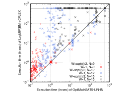
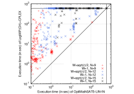
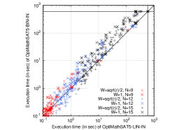
Figure 3: Table: results (# of solved instances, cumulative time in seconds for solved instances) for OptiMathSAT and GAMS (using LogMIP and JAMS) on 100 random instances (including “directly generated” and “encoded” benchmarks) each of the strip-packing problem for $N$ rectangles, where $N=9,12,15$, and width $W=\sqrt{N}/2$, $1$. (We use “OM” as shortcut for OptiMathSAT and omit “+Cplex” in the labels of GAMS tools.) Values highlighted in bold represent best performances. Scatter-plots: comparison of the best configuration of OptiMathSAT (OptiMathSAT-LIN-IN) against LogMIP(BM)+CPLEX (left), LogMIP(CH)+CPLEX (center) and OptiMathSAT-BIN-IN (right) on “directly generated” benchmarks.

Given a set of $N$ rectangles of different length $L_{i}$ and height $H_{i}$, $i\in 1,..,N$, and a strip of fixed width $W$ but unlimited length, the strip-packing problem aims at minimizing the length $L$ of the filled part of the strip while filling the strip with all rectangles, without any overlap and any rotation. (See Figure 2 left.)

The LGDP model provided by [Sawaya and Grossmann (2005)] is the following:

min $$L$$

s.t. $$L\geq x_{i}+L_{i} \forall i\in N$$ (21)

$$\Bigr{[}\begin{array}[]{c}Y^{1}_{ij}\\ x_{i}+L_{i}\leq x_{j}\\ \end{array}\Bigr{]}\vee\Bigr{[}\begin{array}[]{c}Y^{2}_{ij}\\ x_{j}+L_{j}\leq x_{i}\\ \end{array}\Bigr{]}$$

$$\vee\Bigr{[}\begin{array}[]{c}Y^{3}_{ij}\\ y_{i}-H_{i}\geq y_{j}\\ \end{array}\Bigr{]}\vee\Bigr{[}\begin{array}[]{c}Y^{4}_{ij}\\ y_{j}-H_{j}\geq y_{i}\\ \end{array}\Bigr{]} \forall i,j\in N,i<j$$

$$x_{i}\leq\mathsf{ub}-L_{i}\mbox{ } \forall i\in N$$

$$H_{i}\leq y_{i}\leq W\mbox{ } \forall i\in N$$

$$L,x_{i},y_{i}\in\mathbb{R}^{1}_{+},Y_{ij}^{1},Y_{ij}^{2},Y_{ij}^{3},Y_{ij}^{4}\in\{True,False\}$$

where $L$ corresponds to the objective function to minimize and every rectangle $j\in J$ is represented by the constants $L_{j}$ and $H_{j}$ (length and height respectively) and the variables $x_{j},y_{j}$ (the coordinates of the upper left corner in the 2-dimensional space). Every pair of rectangles $i,j\in N,i<j$ is constrained by a disjunction that avoids their overlapping (each disjunct represents the position of rectangle $i$ in relation to rectangle $j$). The size of the strip limits the position of each rectangle $j$: the width of the strip $W$ and the upper bound $\mathsf{ub}$ on the optimal solution bound the $y_{j}$-coordinate and the height $H_{j}$ bounds the $x_{j}$-coordinate. We express straightforwardly the LGDP model (5.2.1) into $\text{OMT}(\mathcal{LA}(\mathbb{Q}))$ as follows:

$$\textstyle\begin{array}[]{lll}\varphi&\stackrel{{\scriptstyle\text{\tiny def}}}{{=}}&({\sf cost}=L)\wedge\bigwedge_{i\in N}(L\geq x_{i}+L_{i})\\ &\wedge&\bigwedge_{i,j\in N,i<j}\Bigl{(}(x_{i}+L_{i}\leq x_{j})\vee(x_{j}+L_{j}\leq x_{i})\\ &&\vee(y_{i}-H_{i}\geq y_{j})\vee(y_{j}-H_{j}\geq y_{i})\Bigr{)}\\ &\wedge&\bigwedge_{i\in N}(x_{i}\leq\mathsf{ub}-L_{i})\wedge\bigwedge_{i\in N}(x_{i}\geq 0)\\ &\wedge&\bigwedge_{i\in N}(H_{i}\leq y_{i})\wedge\bigwedge_{i\in N}(W\geq y_{i})\wedge\bigwedge_{i\in N}(y_{i}\geq 0)\\ \end{array}$$ (32)

We randomly generated instances of the strip-packing problem according to a fixed width $W$ of the strip and a fixed number of rectangles $N$. For each rectangle $j\in N$, length $L_{j}$ and height $H_{j}$ are selected in the interval $]0,1]$ uniformly at random. The upper bound $\mathsf{ub}$ is computed with the same heuristic used by [Sawaya and Grossmann (2005)], which sorts the rectangles in non-increasing order of width and fills the strip by placing each rectangles in the bottom-left corner, and the lower bound $\mathsf{lb}$ is set to zero. We generated 100 samples each for $9$, $10$ and $11$ rectangles and for two values of the width $\sqrt{N}/2$ and $1$ (Notice that with $W=\sqrt{N}/2$ the filled strip looks approximatively like a square, whilst $W=1$ is half the average size of one rectangle. )

5.2.2 The zero-wait jobshop problem.

Procedure	Job-shop
	$I=9,$		$I=10,$		$I=11,$		$I=12,$		$I=11,$		$I=11,$		Total
	$J=8$		$J=8$		$J=8$		$J=8$		$J=9$		$J=10$
	#s.	time	#s.	time	#s.	time	#s.	time	#s.	time	#s.	time	#s.	time
Directly Generated Benchmarks
OM5-LIN-OF	100	386	100	1854	97	9396	57	14051	100	9637	99	10670	553	45995
OM5-LIN-IN	100	317	100	1584	100	8100	77	18046	100	7738	100	7433	577	43228
OM5-BIN-OF	100	726	100	3817	88	13222	38	12529	92	14183	90	13287	508	57764
OM5-BIN-IN	100	602	100	3270	97	12878	54	16234	96	13159	96	12350	543	58493
OM5-ADA-IN	100	596	100	3230	97	12262	53	14810	96	12805	96	12125	542	55828
JAMS(BM)	100	268	100	1113	100	4734	87	17067	100	4941	100	6122	587	34245
JAMS(CH)	84	23830	4	1596	0	0	0	0	0	0	1	363	89	25789
LogMIP(BM)	100	267	100	1114	100	4718	87	17108	100	4962	100	6174	587	34343
LogMIP(CH)	84	23871	4	1622	0	0	0	0	0	0	1	338	89	25831
lgdp2smt Encoded Benchmarks
OM5-LIN-IN	100	324	100	1571	100	7739	74	16494	100	7175	100	7504	574	40807
smt2lgdp1-lgdp2smt Encoded Benchmarks
OM5-LIN-IN	100	336	100	1578	100	7762	71	16589	100	7726	100	7706	571	41697
smt2lgdp2-lgdp2smt Encoded Benchmarks
OM5-LIN-IN	100	320	100	1533	100	7623	68	15120	100	7216	100	7598	568	39410
smt2lgdp1 Encoded Benchmarks
JAMS(BM)	100	239	100	1128	100	5516	84	19949	100	6667	100	4176	584	37675
JAMS(CH)	100	14527	46	17887	0	0	0	0	1	497	0	0	147	32911
LogMIP(BM)	100	240	100	1122	100	5510	83	19489	100	6684	100	4180	583	37225
LogMIP(CH)	100	14465	47	18206	0	0	0	0	1	495	0	0	148	33166
smt2lgdp2 Encoded Benchmarks
JAMS(BM)	100	319	100	1865	100	12470	45	15704	97	13189	96	15773	538	59320
JAMS(CH)	95	22435	18	8030	2	671	0	0	1	526	3	1043	119	32723
LogMIP(BM)	100	319	100	1871	100	12440	45	15747	98	13661	95	15102	538	59140
LogMIP(CH)	95	22401	18	7991	1	163	0	0	1	437	3	1020	118	32012

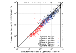
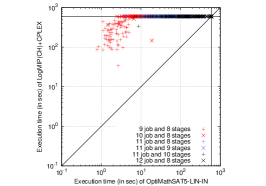
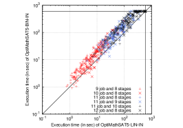
Figure 4: Table: results (# of solved instances, cumulative time in seconds for solved instances) for OptiMathSAT and GAMS on 100 random samples (including “directly generated” and “encoded” benchmarks) each of the job-shop problem for $I=9,10,11,12$ jobs and $J=8$ stages and for $I=11$ jobs and $J=9,10$ stage. (We use “OM” as shortcut for OptiMathSAT and omit “+Cplex” in the labels of GAMS tools.) Values highlighted in bold represent best performances. Scatter-plots: comparison of the best configuration of OptiMathSAT (OptiMathSAT-LIN-IN) against LogMIP(BM)+CPLEX (left), LogMIP(CH)+CPLEX (center) and OptiMathSAT-BIN-IN (right) on “directly generated” benchmarks.

Consider the scenario where there is a set $I$ of jobs which must be scheduled sequentially on a set $J$ of consecutive stages with zero-wait transfer between them. Each job $i\in I$ has a start time $s_{i}$ and a processing time $t_{ij}$ in the stage $j\in J_{i}$, $J_{i}$ being the set of stages of job $i$. The goal of the zero-wait job-shop scheduling problem is to minimize the makespan, that is the total length of the schedule. (See Figure 2 right.)

The LGDP model provided by [Sawaya and Grossmann (2005)] is:

min $$M$$

s.t. $$M\geq\sum_{j\in J_{i}}t_{ij} \forall i\in I$$ (35)

$$\Bigr{[}\begin{array}[]{c}Y^{1}_{ik}\\ s_{i}+\sum_{m\in J_{i},m\leq j}t_{im}\leq s_{k}+\sum_{m\in J_{k},m<j}t_{km}\\ \end{array}\Bigr{]}\vee$$

$$\Bigr{[}\begin{array}[]{c}Y^{2}_{ik}\\ s_{k}+\sum_{m\in J_{k},m\leq j}t_{km}\leq s_{i}+\sum_{m\in J_{i},m<j}t_{im}\\ \end{array}\Bigr{]} \forall j\in C_{ik},\forall i,k\in I,i<k$$

$$M,s_{i}\in\mathbb{R}_{+}^{1},Y^{1}_{ik},Y^{2}_{ik}\in\{True,False\} \forall i,k\in I,i<k$$

where $M$ corresponds to the objective function to minimize and every job $i\in I$ is represented by the variable $s_{i}$ (its start time) and the constant $t_{ij}$ (its processing time in stage $j\in J_{i}$). For each pair of jobs $i,k\in I$ and for each stage $j$ with potential clashes (i.e $j\in C_{ik}=\{J_{i}\cap J_{k}\}$), a disjunction ensures that no clash between jobs occur at any stage at the same time. We encoded the corresponding LGDP model (5.2.2) into $\text{OMT}(\mathcal{LA}(\mathbb{Q}))$ as follows:

$$\textstyle\begin{array}[]{lll}\varphi&\stackrel{{\scriptstyle\text{\tiny def}}}{{=}}&({\sf cost}=M)\wedge\bigwedge_{i\in I}(M\geq s_{i}+\sum_{j\in J_{i}}t_{ij})\wedge\bigwedge_{i\in I}(s_{i}\geq 0)\\ &\wedge&\bigwedge_{j\in C_{ik},\forall i,k\in I,i<k}\left((s_{i}+\sum_{m\in J_{i},m\leq j}t_{im}\leq s_{k}+\sum_{m\in J_{k},m<j}t_{km})\right.\\ &&\hskip 85.35826pt\vee\left.(s_{k}+\sum_{m\in J_{k},m\leq j}t_{km}\leq s_{i}+\sum_{m\in J_{i},m<j}t_{im})\right)\\ \end{array}-$$ (42)

We generated randomly instances of the zero-wait jobshop problem according to a fixed number of jobs $I$ and a fixed number of stages $J$. For each job $i\in I$, start time $s_{i}$ and processing time $t_{ij}$ of every job are selected in the interval $]0,1]$ uniformly at random. We consider a set of 100 samples each for 9, 10, 11, 12 jobs and 8 stages and for 11 jobs and 9, 10 stages. We set no value for $\mathsf{ub}$ and $\mathsf{lb}=0$.

5.2.3 Discussion

The table of Figure 3 shows the number of solved instances and their cumulative execution time for different configurations of OptiMathSAT and GAMS on “directly generated” and “encoded” benchmarks. The scatter-plots of Figure 3 compare the best-performing version of OptiMathSAT, OptiMathSAT-LIN-IN, against LogMIP+CPLEX with BM and CH reformulation (left and center respectively) and the two inline versions OptiMathSAT-LIN-IN and OptiMathSAT-BIN-IN (right) on “directly generated” benchmarks.

The table of Figure 4 shows the number of solved instances and their cumulative execution time for different configurations of OptiMathSAT and GAMS on “directly generated” and “encoded” benchmarks. The scatter-plots of Figure 4 compare, on “directly encoded” benchmarks, the best-performing version of OptiMathSAT, OptiMathSAT-LIN-IN, against LogMIP with BM and CH reformulation (left and center respectively); the figure also compares the two inline versions OptiMathSAT-LIN-IN and OptiMathSAT-BIN-IN (right).

The results on the LGDP problems in Figures 3, 4 suggest some considerations.

Comparing the different versions of OptiMathSAT, we notice that:

• the inline versions (-IN) behave pairwise uniformly better than the corresponding offline versions (-OF), which is not surprising;

• overall the -LIN options seems to perform a little better than the corresponding -BIN and -ADA options (although gaps are not dramatic).

Remark 5.3.

We notice that with LGDP problems binary search is not “obviously faster” than linear search, in compliance with what stated in point 6. in §4.1. This is further enforced by the fact that in strip-packing (32) [resp. job-shop (42)] encodings, the cost variables ${\sf cost}\stackrel{{\scriptstyle\text{\tiny def}}}{{=}}L$ [resp. ${\sf cost}\stackrel{{\scriptstyle\text{\tiny def}}}{{=}}M$] occurs only in positive unit clauses in the form $(L\geq\langle{term}\rangle)$ [resp. $(M\geq\langle{term}\rangle)$]; thus, learning $\neg({\sf cost}<\mathsf{pivot})$ as a result of the binary-search steps with unsat results produces no constraining effect on the variables in $\langle{term}\rangle$, and hence no substantial extra search-pruning effect due to the early-pruning technique of the SMT solver.

Comparing the different versions of the GAMS tools, we see that LogMIP and JAMS reformulations lead to substantially identical performance on both strip-packing and job-shop instances. For both reformulation tools, the BM versions uniformly outperform the CH ones, often dramatically.

Comparing the performances of the versions of OptiMathSAT against these of the GAMS tools, we notice that

• on strip-packing problems all versions of OptiMathSAT outperform all GAMS versions, regardless of the encoding used. E.g., the best OptiMathSAT version solved $\approx 30\%$ more formulas than the best GAMS version;

• on job-shop problems results are mixed. OptiMathSAT drastically outperforms the CH versions on all encodings and it slightly beats the BM ones on “smt2lgdp₂ encoded” benchmarks, whilst it is slightly beaten by the BM versions on “directly generated” and “smt2lgdp₁ encoded” benchmarks. E.g., the best OptiMathSAT version solved $\approx 2\%$ less formulas than the best GAMS version.

Overall, we can conclude that OptiMathSAT performances on these problems are comparable with, and most often significantly better than, those of GAMS tools.

We may wonder how these results are affected by the different encodings used. (We recall from the beginning of §5 that all solvers agreed on the results, regardless of the encoding.) In terms of performances, comparing the effects of the different encodings, we notice the following facts.

• On OptiMathSAT (-LIN-IN) the effects of the different encodings is substantially negligible, on both strip-packing and job-shop problems, since we have only very small variations in the number of solved instances between “directly generated” and “encoded” instances, in the various encoding combinations. From this reason, we conclude that OptiMathSAT is robust wrt. the encodings of these problems.

• On GAMS tools the effects of the different encodings are more relevant, although very heterogeneous: e.g., wrt. to “directly generated” instances, “smt2lgdp₁ encoded” solved formulas are slightly less with BM options, and up to much more with CH options; “smt2lgdp₂ encoded” solved formulas are slightly more on strip-packing and a little less on job-shop with BM options, slightly less on strip-packing and a much more on job-shop with CH options. For this reason, in next sections we always report the results with both encodings.

solving/total time ratio	minimization/total time ratio	certification/total time ratio

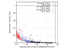
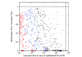
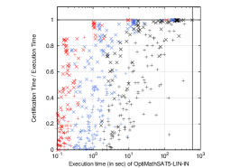
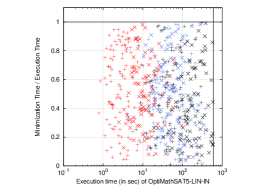
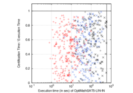
Figure 5: Scatter-plots comparing solving, minimization and certification time (left, center and right respectively) with the execution time of OptiMathSAT-LIN-IN on “directly generated” instances of strip-packing (top) and job-shop (bottom).

5.2.4 Analysis of OptiMathSAT performances.

We want to perform a more fine-grained analysis of the performances of the best version of OptiMathSAT, OptiMathSAT-LIN-IN. To this extent, we partition the total execution time taken on each problem into three consecutive components:

• solving time, i.e. the time spent on finding the first sub-optimal solution,

• minimization time, i.e. the time required to search for the optimal solution,

• and certification time, i.e. the time needed for checking there is no better solution.

Figure 5 reports, for all strip-packing (top) and job-shop (bottom) instances, the ratios of the three components above over total execution time. (Notice the log scale of the x axis and the linear scale on the y axis.) We notice a few facts:

• the solving time is nearly negligible, in particular on hardest problems. This tells us, among other facts, that $\text{OMT}(\mathcal{LA}(\mathbb{Q}))$ on these formulas is a much harder problem that plain $\text{SMT}(\mathcal{LA}(\mathbb{Q}))$ on the same formulas;

• the remaining time, on average, is either evenly shared between the minimization and the certification efforts (job-shop, bottom) or even it is mostly dominated by the latter, in particular on the hardest problem (strip-packing, top).

Overall, this suggests that on these instances OptiMathSAT-LIN-IN takes on average less than half of the total execution time to find the actual optimal solution, and more than half to prove that there is no better one.

5.3 Comparison on SMT-LIB problems

Procedure	SMT-LIB/QF_LRA formulas
	#inst.	#term.	#correct.	#err.msg.	#wrong	#unfeas.	time
OptiMathSAT5-LIN-IN	194	194	194	0	0	0	1604
OptiMathSAT5-BIN-IN	194	194	194	0	0	0	1449
OptiMathSAT5-ADA-IN	194	194	194	0	0	0	1618
LDGP-SMT-Encoded Benchmarks (smt2lgdp1-lgdp2smt)
OptiMathSAT5-LIN-IN	194	194	194	0	0	0	1820
LDGP-SMT-Encoded Benchmarks (smt2lgdp2-lgdp2smt)
OptiMathSAT5-LIN-IN	194	194	194	0	0	0	1597
LGDP-Encoded Benchmarks (smt2lgdp1)
JAMS(BM)+CPLEX	194	171	116	52	0	3	1561
JAMS(CH)+CPLEX	194	193	15	108	0	70	559
LogMIP(BM)+CPLEX	194	172	117	52	0	3	2152
LogMIP(CH)+CPLEX	194	193	15	108	0	70	576
LGDP-Encoded Benchmarks (smt2lgdp2)
JAMS(BM)+CPLEX	194	172	166	0	4	2	6839
JAMS(CH)+CPLEX	194	105	104	0	0	1	9912
LogMIP(BM)+CPLEX	194	171	165	0	4	2	4103
LogMIP(CH)+CPLEX	194	105	104	0	0	1	9649

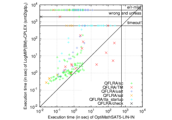
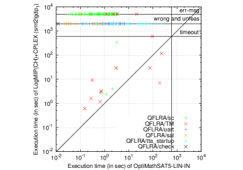
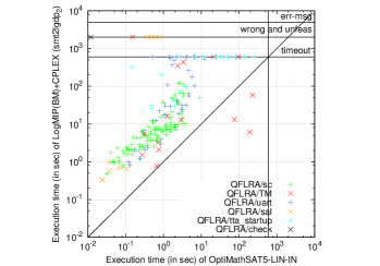
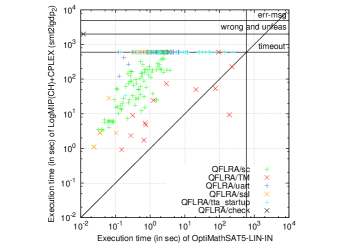
Figure 6: Table: Results for all the inline versions of OptiMathSAT and all the GAMS tools, on a subset of SMT-LIB $\mathcal{LA}(\mathbb{Q})$ satisfiable instances. The columns report respectively: # of instances considered, # of instances terminating within the timeout, # of instances terminating with correct solution, # of instances terminating with error messages, # of instances terminating returning a wrong minimum, # of instances terminating wrongly returning “unfeasible”. Scatter-plots: pairwise comparisons on the smt-lib $\mathcal{LA}(\mathbb{Q})$ satisfiable instances between OptiMathSAT-LIN-IN and the two versions of LogMIP+CPLEX. LGDP models are generated using smt2lgdp₁ (top) and smt2lgdp₂ (bottom).

As a second comparison, in Figure 6 we compare OptiMathSAT against the GAMS tools on the satisfiable $\mathcal{LA}(\mathbb{Q})$-formulas (QF_LRA) in the SMT-LIB, augmented with randomly-selected costs. (Hereafter we do not consider the -OF versions of OptiMathSAT.) These instances are all classified as “industrial”, because they come from the encoding of different real-world problems in formal verification, planning and optimization. They are divided into six categories, namely: sc, uart, sal, TM, tta_startup, and miplib. Notice that other SMT-LIB categories like spider_benchmarks and clock_synchro do not contain satisfiable instances and are thus not reported here.

Since we have no control on the origin of each problem and on the name and meaning of the variables, we selected iteratively one variable at random as ${\sf cost}$ variable, dropping it if the resulting minimum was $-\infty$. This forced us to eliminate a few instances, in particular all miplib ones. We used both smt2lgdp₁ and smt2lgdp₂ to encode these problems into LGDP.

As before, to check for both correctness and effectiveness of the encodings, we also encoded the problems into LGDP by each encoding and encoded then back, to be fed to OptiMathSAT-LIN-IN (4th and 5th row). We notice that this caused substantial difference in neither correctness nor efficiency.

We notice first that the results for GAMS tools are affected by correctness problems, with both encodings. Consider the encoding smt2lgdp₁. Out of 194 samples, both GAMS tools with the CH option returned “unfeasible” (i.e. inconsistent) on 70 samples and an error message (regarding some unsatisfied disjunctions) on 108 samples. The two versions with BM returned 3 unfeasible solutions and 52 solutions with error messages. Only 15 samples were solved correctly by GAMS tools with the CH option and $117$ (with LogMIP) or $116$ (with JAMS) samples with BM ones, whilst OptiMathSAT solved correctly all 194 samples. (We recall that all OptiMathSAT results were cross-checked, and that the four GAMS tools were fed with the same files.) With smt2lgdp₂ encoding the number of correctly-solved formulas increases, $104$ with CH option and $165$ (with LogMIP) or $166$ (with JAMS) with BM; there are no error messages and the number of unfeasible solutions of both GAMS tools with the BM and CH options decreases to 2 and 1 respectively, but the number of solutions with wrong minimum increases to 4 with the BM versions.

Importantly, with both encodings, the results for GAMS tools varied by modifying a couple of parameters from their default value, namely “eps” and “bigM Mvalue”. For example, on the above-mentioned sal instance with smt2lgdp₁, with the default values the BM versions returned a wrong minimum value “0”, the CH versions returned “unfeasible”, whilst OptiMathSAT returned the correct minimum value “2”; modifying eps and bigM Mvalue, the results become unfeasible also with BM options. This highlights the fact that there are indeed some correctness and robustness problems with the GAMS tools, regardless of the encodings used.  

solving/total time ratio	minimization/total time ratio	certification/total time ratio

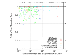
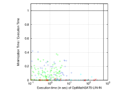
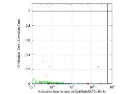
Figure 7: Scatter-plots comparing solving, minimization and certification time (left, center and right respectively) with the execution time of OptiMathSAT-LIN-IN on SMT-LIB instances.

5.3.1 Discussion

We conjecture that the problems with the GAMS tools may be caused, at least in part, by the fact that GAMS tools use floating-point rather than infinite-precision arithmetic, and they introduce internally an approximated representation of strict inequalities (see Remark 5.1). Notice that, unlike with the LGDP problems in §5.2, SMT-LIB problems do contain occurrences of strict [resp. non-strict] inequalities with positive [resp. negative] polarity.

From the perspective of the efficiency, all versions of OptiMathSAT solved correctly all problems within the timeout, the -BIN-IN version performing slightly better than the others; GAMS did not solve many samples (because of timeout, wrong solutions and solutions with error messages). Looking at the scatter-plots, we notice that, with the exception of a few samples, OptiMathSAT always outperforms the GAMS tools, often by more than one order magnitude. We notice that on these problems smt2lgdp₂ is generally more effective than smt2lgdp₁ and less prone to errors.

Finally, Figure 7 reports for all SMT-LIB instances the ratios of the solution, minimization and certification times over the total execution time for OptiMathSAT-LIN-IN. Unlike with Figure 5, we notice that here the solution time is dominating, the minimization time is significant, and the certification time is nearly negligible. This means that on these instances OptiMathSAT-LIN-IN takes on average more than half of its execution time to find the first solution, less than half to find the actual optimal solution, and very little time to prove that there is no better one. We conjecture that this is due to the fact that most satisfiable SMT-LIB instances come from the encoding of formal verification steps of bugged systems which, unlike with the LGDP problems of §5.2, have a limited number of solutions.

5.4 Comparison on SAL problems

Procedure	SAL formulas
	#inst.	#term.	#correct	#err. msg.	#wrong	#unfeas.	time
OptiMathSAT5-LIN-IN	392	385	385	0	0	0	44129
OptiMathSAT5-BIN-IN	392	382	382	0	0	0	45869
OptiMathSAT5-ADA-IN	392	381	381	0	0	0	44932
LGDP-Encoded Benchmarks (smt2lgdp1)
JAMS(BM)+CPLEX	392	24	4	19	1	0	1096
JAMS(CH)+CPLEX	392	46	0	0	0	46	0
LogMIP(BM)+CPLEX	392	24	4	19	1	0	1092
LogMIP(CH)+CPLEX	392	46	0	0	0	46	0
LGDP-Encoded Benchmarks (smt2lgdp2)
JAMS(BM)+CPLEX	392	28	14	0	14	0	1456
JAMS(CH)+CPLEX	392	31	2	0	0	29	122
LogMIP(BM)+CPLEX	392	28	14	0	14	0	1428
LogMIP(CH)+CPLEX	392	31	2	0	0	29	120

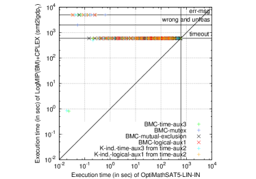
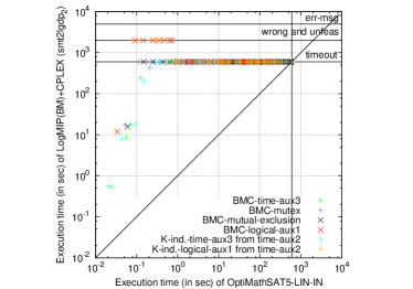
Figure 8: Table: Results for all the inline versions of OptiMathSAT and all the GAMS tools, on formulas generated from SAL models of Fisher’s protocol. The columns report respectively: # of instances considered, # of instances terminating within the timeout, # of instances terminating with correct solution, # of instances terminating with error messages (GAMS tools only), # of instances terminating returning a wrong minimum, # of instances terminating wrongly returning “unfeasible”. Scatter-plots: comparison of the best configuration of OptiMathSAT (OptiMathSAT-LIN-IN) against LogMIP(BM)+CPLEX on smt2lgdp₁ and smt2lgdp₂ encodings (left and right respectively).

As a third comparison, in Figure 8 we compare OptiMathSAT against the GAMS tools on $\mathcal{LA}(\mathbb{Q})$-formulas obtained by using the SAL Model Checker on a set of bounded verification problems — Bounded Model Checking (BMC) of invariants [Biere et al. (1999)] and K-Induction (K-ind) [Sheeran et al. (2000)] — of a well-known parametric timed system, Fisher’s Protocol .

BMC [resp. K-ind ] takes a Finite-State Machine $M$, an invariant property $\Psi$ and an integer bound $k$, and produces a propositional formula $\varphi$ which is satisfiable [resp. unsatisfiable] if and only if there exists a $k$-step execution violating $\Psi$ [resp. a $k$-step induction proof that $\Psi$ is always verified]. The approach leverages to real-time systems by producing $\text{SMT}(\mathcal{LA}(\mathbb{Q}))$ formulas rather than purely-propositional ones (see, e.g., [Audemard et al. (2002)]).

Fisher’s Protocol ensures mutual exclusion among $N$ processes using real-time clocks and a shared variable. The problem is parametric into two positive real values, $\delta_{1}$ and $\delta_{2}$, describing the delays of some actions. It is known that mutual exclusion, and other properties included in the SAL model, are verified if and only if $\delta_{1}<\delta_{2}$.

We have produced our $\text{OMT}(\mathcal{LA}(\mathbb{Q}))$ problems as follows. We fixed the value of $\delta_{2}$ (we chose $\delta_{2}=4$), and then we generated six groups of formulas according to the problem solved (BMC or K-ind) and the property addressed (called mutex, mutual-exclusion, time-aux3 and logical-aux1). For each group, for increasing values of $N\geq 2$ and for a set of sufficiently-big values of $k\geq k^{*}$,  we used SAL to produce the corresponding parametric $\text{SMT}(\mathcal{LA}(\mathbb{Q}))$ formulas, and asked the tool under test to find the minimum value of $\delta_{1}$ which made the resulting formula $\mathcal{LA}(\mathbb{Q})$-satisfiable (we knew in advance from the problem that, for $k$ big enough, this value is $\delta_{1}=\delta_{2}=4.0$). As before, we used both smt2lgdp₁ and smt2lgdp₂ to encode the $\text{OMT}(\mathcal{LA}(\mathbb{Q}))$ benchmarks into LGDP.

5.4.1 Discussion

The results are presented in Figure 8. The three versions of OptiMathSAT solved correctly 385, 382 and 381 out of the 392 samples respectively, OptiMathSAT-LIN-IN being the best performer.

Considering the GAMS tools with the encoding smt2lgdp₁, the two tools using BM solved on time and correctly only 4 samples over 392 and returned 19 solutions with error messages and 1 solution with wrong minimum, whilst the CH ones always returned “unfeasible”. (We recall that all GAMS tools and options are fed the same inputs.) Considering the encoding smt2lgdp₂, the GAMS tools solved more problems correctly (14 with BM tools and 2 with CH), but they returned wrong and unfeasible solutions (14 wrong solutions for BM versions and 29 unfeasible for CH ones). No solution with error messages was found.

The scatter-plots compare OptiMathSAT-LIN-IN with the best versions of GAMS, LogMIP(BM)+CPLEX, on both the encodings, showing that the former dramatically outperforms the latter, no matter the encoding used.

5.5 Comparison on pseudo-Boolean SMT problems

Procedure	MaxSMT $/$ SMT+PB problems
	#inst.	#term.	#correct.	#err.msg.	#wrong	#unfeas.	time
PB-MathSAT-LIN	675	636	636	0	0	0	19675
PB-MathSAT-BIN	675	632	632	0	0	0	13024
$\text{OMT}(\mathcal{LA}(\mathbb{Q}))$-Encoded Benchmarks
OptiMathSAT-LIN-IN	675	630	630	0	0	0	20744
OptiMathSAT-BIN-IN	675	634	634	0	0	0	16502
OptiMathSAT-ADA-IN	675	637	637	0	0	0	18588
LGDP-Encoded Benchmarks (smt2lgdp1)
JAMS(BM)+CPLEX	675	509	19	423	68	8	420
JAMS(CH)+CPLEX	675	642	0	233	41	377	0
LogMIP(BM)+CPLEX	675	510	19	424	68	8	403
LogMIP(CH)+CPLEX	675	642	0	233	41	377	0
LGDP-Encoded Benchmarks (smt2lgdp2)
JAMS(BM)+CPLEX	675	449	92	9	351	6	1575
JAMS(CH)+CPLEX	675	386	48	9	336	2	644
LogMIP(BM)+CPLEX	675	449	92	9	351	6	1650
LogMIP(CH)+CPLEX	675	383	48	9	333	2	674

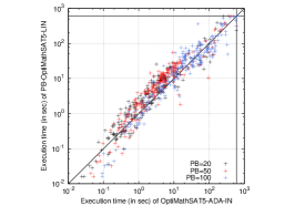
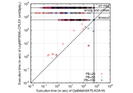
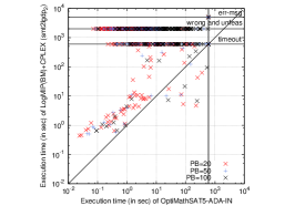
Figure 9: Table: Results for OptiMathSAT, PB-MathSAT and the GAMS tools, on the MaxSMT benchmarks from [Cimatti et al. (2010)]. The columns report respectively: # of instances considered, # of instances terminating within the timeout, # of instances terminating with correct solution, # of instances terminating with error messages (GAMS tools only), # of instances terminating returning a wrong minimum, # of instances terminating wrongly returning “unfeasible”. Scatter-plots: comparison of the best configuration of OptiMathSAT, OptiMathSAT-ADA-IN, against the best configuration of PB-MathSAT, PB-MathSAT-LIN (left) and the best configuration of GAMS tools, LogMIP(BM)+CPLEX, on smt2lgdp₁ and smt2lgdp₂ encodings (center and right respectively).

As a fourth comparison, in Figure 9 we evaluate OptiMathSAT on the problem sets used in [Cimatti et al. (2010)] against the usual GAMS tools and against a recent reimplementation on MathSAT5 of the tool in [Cimatti et al. (2010)], namely PB-MathSAT, for SMT with Pseudo-Boolean constraints (see §3). PB-MathSAT is tested with both linear search and binary search strategies (denoted with “-LIN” and “-BIN” respectively).

As described in [Cimatti et al. (2010)], the problems consists of partial weighted MaxSMT problems which are generated randomly starting from satisfiable $\mathcal{LA}(\mathbb{Q})$-formulas (QF_LRA) in the SMT-LIB, then converted into SMT problems with PB constraints, see (15) in §3. These problems are further encoded into $\text{OMT}(\mathcal{LA}(\mathbb{Q}))$ problems by means of the encoding (14) in §3, and hence into LGDP problems by means of the usual two encodings.

5.5.1 Discussion

The results are presented in Figure 9. The three versions of OptiMathSAT solved respectively 630, 634 and 637 problems out of 675 problems overall, whilst the two versions PB-MathSAT solved respectively 636 and 632. Thus, despite they are both implemented on top of the same SMT solver and PB-MathSAT is specialized for PB constraints, OptiMathSAT performances are analogous to these of the more-specialized tool. The various version of the GAMS tool perform drastically worse: with smt2lgdp₁ they solve correctly only a very small number of samples (19 with BM tools and even 0 with CH), returning error messages, unfeasible results or wrong minimum solutions on the remaining set of benchmarks; with smt2lgdp₂ more samples are solved correctly and no error message is produced, but most problems produce a wrong minimum solution.

Remark 5.4.

Notice that, unlike with LGDP problems (see Remark 5.3) and in part also with SMT-LIB and SAL problems, with Pseudo-Boolean problems the cost variables occurs in positive unit clauses in the form $({\sf cost}=\langle{term}\rangle)$; thus, learning $\neg({\sf cost}<\mathsf{pivot})$ as a result of the binary-search steps with unsat results produces a constraining effect on the variables in $\langle{term}\rangle$, and hence a pruning effect in the search due to the early-pruning technique of the SMT solver. This might explain in part the fact that, unlike with previous problems, here binary search performs a little better than linear search.

The scatter-plots in Figure 9 compare the best version of OptiMathSAT with these of PB-MathSAT and of the GAMS tools. We see that OptiMathSAT-ADA-IN performances are analogous to these of PB-MathSAT-LIN, and they are drastically superior to these of GAMS tools with both encodings.

As a side note, in [Cimatti et al. (2013a)] another empirical evaluation is performed on MaxSMT problems —although generated with a slightly different random method from SMT-LIB benchmarks— where OptiMathSAT performs equivalently better than PB-MathSAT and the novel specialized MaxSMT tool presented there. We refer the reader to [Cimatti et al. (2013a)] for details.

5.6 Comparison against GAMS with parallel Cplex on all problem sets

Procedure	#inst.	#term.	#correct	#err. msg.	#wrong	#unfeas.	time	average
								speedup
Strip-packing LGDP problems (Directly Generated Benchmarks)
OptiMathSAT-LIN-IN	600	568	568	0	0	0	12782	–
JAMS(BM)+CPLEX	600	432	432	0	0	0	22318	–
JAMS(BM)+CPLEX-4cores	600	472	472	0	0	0	17918	5.98
Job-shop LGDP problems (Directly Generated Benchmarks)
OptiMathSAT-LIN-IN	600	577	577	0	0	0	43228	–
JAMS(BM)+CPLEX	600	587	587	0	0	0	34245	–
JAMS(BM)+CPLEX-4cores	600	600	600	0	0	0	10465	9.54
SMT-LIB problems (LGDP-Encoded Benchmarks (smt2lgdp2))
OptiMathSAT5-LIN-IN	194	194	194	0	0	0	1604	–
JAMS(BM)+CPLEX	194	172	166	0	4	2	6839	–
JAMS(BM)+CPLEX-4cores	194	155	150	0	4	1	2990	2.36
SAL problems (LGDP-Encoded Benchmarks (smt2lgdp2))
OptiMathSAT5-LIN-IN	392	385	385	0	0	0	44129	–
JAMS(BM)+CPLEX	392	28	14	0	14	0	1456	–
JAMS(BM)+CPLEX-4cores	392	32	17	0	15	0	786	3.66
MaxSMT $/$ SMT+PB problems (LGDP-Encoded Benchmarks (smt2lgdp2))
OptiMathSAT-LIN-IN	675	630	630	0	0	0	20744	–
JAMS(BM)+CPLEX	675	449	92	9	351	6	1575	–
JAMS(BM)+CPLEX-4cores	675	479	95	9	367	6	4033	2.35

Strip-packing LGDP	Job-shop LGDP
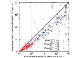
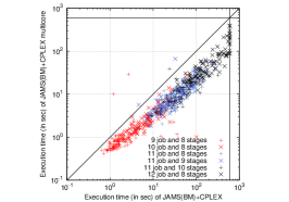
SMT-LIB	SAL	MaxSMT / SMT+PB

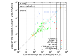
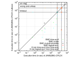
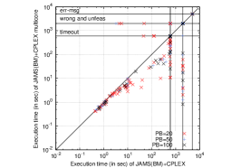
Figure 10: Table: comparison of OptiMathSAT-LIN-IN, JAMS(BM)+CPLEX and JAMS(BM)+CPLEX-4cores on the five problem sets. Last column: average speedup for JAMS(BM)+CPLEX-4cores wrt. JAMS(BM)+CPLEX. Scatterplots: pairwise comparison of JAMS(BM)+CPLEX-4cores vs. JAMS(BM)+CPLEX on the five problem sets.

As it is common practice in the SMT literature, in this paper we deal with single-core sequential procedures. In fact, despite a couple of attempts [Wintersteiger et al. (2009), Kalinnik et al. (2010)], the parallelization of SMT-solving procedures is still an open research issue. In particular MathSAT5, and hence OptiMathSAT, provide no support for parallelization. Thus, although the issue of efficiently parallelizing OMT is potentially a very interesting research topic, it is definitely not in the intended scope of this paper.

Unlike with MathSAT5 and OptiMathSAT, however, Cplex provides full support for multiple-core parallel solving. This is an important benefit, since it allows for exploiting the multiple-core CPUs of current PCs, reducing the elapsed time when searching for a solution. This gives GAMS a potential advantage wrt. OptiMathSAT which the previous tests could not reveal.

In order to investigate the actual relevance of this potential advantage, we have recently enriched our empirical investigation by running all the tests in §5.2-§5.5 also on another GAMS tool, namely JAMS(BM)+CPLEX-4cores: this is the best-performing GAMS GAMS tool in the tests, JAMS(BM)+CPLEX, which uses instead the most recent version of Cplex, v12.6, in parallel mode on four cores (options opportunistic parallelmode, 4 threads). Each of the four threads is given a timeout of 600s. Therefore JAMS(BM)+CPLEX-4cores is given four times the CPU time resources than its competitors.

5.6.1 Discussion

The results are displayed in Figure 10. In the table, for each group of benchmarks in §5.2-§5.5, we compare the performances of the best-performing OptiMathSAT tool, OptiMathSAT-LIN-IN, of the best-performing GAMS tool, JAMS(BM)+CPLEX, and of its parallel version, JAMS(BM)+CPLEX-4cores. The results for the former two tools are taken from Figures 3-9. In the last column we report the mean values of the speedup for JAMS(BM)+CPLEX-4cores wrt. JAMS(BM)+CPLEX over the problems for which both tools terminated within the timeout. In the scatterplots we compare pairwise the performances of JAMS(BM)+CPLEX-4cores and JAMS(BM)+CPLEX on the five problem sets.

From Figure 10 we notice the following facts.

• The usage of Cplex in parallel mode on the four cores pays off in terms of elapsed time: we notice a significant average speedup from JAMS(BM)+CPLEX to JAMS(BM)+CPLEX-4cores, ranging from $2.35$ to $9.54$ with the five problem sets.

• The speedup is high and reasonably regular for the two LGDP problem sets, it is lower and quite irregular for the other three problem sets.

• The speedup does not change the qualitative results of the evaluation in the previous sections: OptiMathSAT still performs better than all GAMS tools, including JAMS(BM)+CPLEX-4cores, on the Strip-packing, SMT-LIB, SAL and MaxSMT/SMT+PB problems sets, it performs worse on the Job-shop problem set.

Overall we can conclude that OptiMathSAT is very competitive with, and often outperforms, GAMS LGDP tools on the very-extensive set of problems we have used to evaluate them, despite the possibility of GAMS to use Cplex in parallel mode on multiple-core CPUs. This clearly demonstrates the potential of our novel OMT approach.

6 Related work.

The idea of optimization in SMT was first introduced by Nieuwenhuis & Oliveras [Nieuwenhuis and Oliveras (2006)], who presented a very-general logical framework of “SMT with progressively stronger theories” (e.g., where the theory is progressively strengthened by every new approximation of the minimum cost), and present implementations for MaxSMT based on this framework.

Cimatti et al. [Cimatti et al. (2010)] introduced the notion of “Theory of Costs” $\mathcal{C}$ to handle PB cost functions and constraints by an ad-hoc and independent “$\mathcal{C}$-solver” in the standard lazy SMT schema, and implemented a variant of MathSAT tool able to handle SMT with PB constraints and to minimize PB cost functions.

The SMT solvers Yices [Dutertre and Moura (2006)] and Z3 [de Moura and Bjørner (2008)] also provide support for MaxSMT, although there is no publicly-available document describing the procedures used there.

Ansótegui et al. [Ansótegui et al. (2011)] describe the evaluation of an implementation of a MaxSMT procedure based on Yices, although this implementation is not publicly available.

Cimatti et al. [Cimatti et al. (2013a)] presented a “modular” approach for MaxSMT, combining a lazy SMT solver with a MaxSAT solver, which can be used as blackboxes.

We recall that MaxSMT and SMT with PB functions can be encoded into each other, and that both are strictly less general than the problem addressed in this paper (§3).

Two other forms of optimization in SMT, which are quite different from the one presented in our work, have been proposed in the literature.

Dillig et al. [Dillig et al. (2012)] addressed the problem of finding partial models for quantified first-order formulas modulo theories, which minimize the number of free variables which are assigned a value from the domain.Quoting an example from [Dillig et al. (2012)], given the formula $\varphi\stackrel{{\scriptstyle\text{\tiny def}}}{{=}}(x+y+w>0)\vee(x+y+z+w<5)$, the partial assignment $\{z=0\}$ satisfies $\varphi$ because every total assignment extending it satisfies $\varphi$ and is minimum because there is no assignment satisfying $\varphi$ which assigns less then one variable. They proposed a general procedure addressing the problem for every theory $\mathcal{T}$ admitting quantifier elimination, and implemented a version for $\mathcal{LA}(\mathbb{Z})$ and $\mathcal{EUF}$ into the Mistral tool.

Manolios and Papavasileiou [Manolios and Papavasileiou (2013)] proposed the “ILP Modulo Theories” framework as an alternative to SAT Modulo Theories, which allows for combining Integer Linear Programming with decision procedures for signature-disjoint stably-infinite theories $\mathcal{T}$; they presented a general algorithm by integrating the Branch&Cut ILP method with $\mathcal{T}$-specific decision procedures, and implemented it into the Inez tool. Notice that the approach of [Manolios and Papavasileiou (2013)] cannot combine ILP with $\mathcal{LA}(\mathbb{Q})$, since $\mathcal{LA}(\mathbb{Z})$ and $\mathcal{LA}(\mathbb{Q})$ are not signature-disjoint. (See Definition 2 in [Manolios and Papavasileiou (2013)].) Also, the objective function is defined on the Integer domain.

We understand that neither of the above-mentioned works can handle the problem addressed in this paper, and vice versa. 

7 Conclusions and Future Work

In this paper we have introduced the problem of $\text{OMT}(\mathcal{LA}(\mathbb{Q})\cup\mathcal{T})$, an extension of $\text{SMT}(\mathcal{LA}(\mathbb{Q})\cup\mathcal{T})$ with minimization of $\mathcal{LA}(\mathbb{Q})$ terms, and proposed two novel procedures addressing it. We have described, implemented and experimentally evaluated this approach, clearly demonstrating all its potentials. We believe that $\text{OMT}(\mathcal{LA}(\mathbb{Q})\cup\mathcal{T})$ and its solving procedures propose as a very-promising tools for a variety of optimization problems.

This research opens the possibility for several interesting future directions. A short-term goal, which we are currently working at, is to extend the approach to $\mathcal{LA}(\mathbb{Z})$ and to mixed $\mathcal{LA}(\mathbb{Q})$/$\mathcal{LA}(\mathbb{Z})$, by exploiting the solvers which are already present in MathSAT [Griggio (2012)]. As it is implicitly suggested in §5.6, a medium-term goal is to investigate the parallelization of OMT procedures, so that to exploit the power of current multiple-core CPUs. A longer-term goal is to investigate the feasibility of extending the technique to deal with non-linear constraints, possibly using MINLP tools as $\mathcal{T}$-$\mathsf{Solver}$/$\mathsf{Minimize}$.

Appendix A Appendix: Proof of the Theorems

A.1 Proof of Theorem 3.6

We first need proving the following lemmas.

Lemma A.1.

Let $\varphi$ be a $\mathcal{LA}(\mathbb{Q})\cup\mathcal{T}$-satisfiable $\mathcal{LA}(\mathbb{Q})\cup\mathcal{T}$-formula and $\mathcal{E}\stackrel{{\scriptstyle\text{\tiny def}}}{{=}}\{\eta_{1},\ldots,\eta_{n}\}$ be the set of all total truth assignments propositionally satisfying $\varphi$. Then $\mathsf{min}_{\sf cost}(\varphi)=min_{\eta_{i}\in\mathcal{E}}\mathsf{min}_{\sf cost}(\eta_{i})$.

Proof A.2.

If $\varphi$ is $\mathcal{LA}(\mathbb{Q})\cup\mathcal{T}$-unsatisfiable, then $\mathsf{min}_{\sf cost}(\varphi)=min_{\eta_{i}\in\mathcal{E}}\mathsf{min}_{\sf cost}(\eta_{i})=+\infty.$ Otherwise, the thesis follows straightforwardly from the fact that the set of the models of $\varphi$ is the union of the sets of the models of the assignments in $\mathcal{E}$. ∎

Lemma A.3.

Let $\varphi$ be a $\mathcal{LA}(\mathbb{Q})\cup\mathcal{T}$-satisfiable $\mathcal{LA}(\mathbb{Q})\cup\mathcal{T}$-formula and $\mu$ be a $\mathcal{LA}(\mathbb{Q})\cup\mathcal{T}$-satisfiable partial assignment s.t. $\mu\models_{p}\varphi$. Then there exists at least one $\mathcal{LA}(\mathbb{Q})\cup\mathcal{T}$-satisfiable total assignment $\eta$ s.t. $\mu\subseteq\eta$, $\eta\models_{p}\varphi$, and $\mathsf{min}_{\sf cost}(\mu)=\mathsf{min}_{\sf cost}(\eta)$.

Proof A.4.

Let $\mathcal{I}$ be a model for $\mu$, and hence for $\varphi$. Then

$$\eta\stackrel{{\scriptstyle\text{\tiny def}}}{{=}}\bigwedge_{\stackrel{{\scriptstyle\psi_{i}\in Atoms(\varphi)}}{{\mathcal{I}\models\psi_{i}}}}\psi_{i}\wedge\bigwedge_{\stackrel{{\scriptstyle\psi_{i}\in Atoms(\varphi)}}{{\mathcal{I}\models\neg\psi_{i}}}}\neg\psi_{i}$$ (43)

By construction, $\eta$ is a total truth assignment for $\varphi$ and it is $\mathcal{LA}(\mathbb{Q})\cup\mathcal{T}$-satisfiable, $\mu\subseteq\eta$ and $\mathsf{min}_{\sf cost}(\eta)=\mathsf{min}_{\sf cost}(\mu)=\mathcal{I}({\sf cost})$. Since $\mu\subseteq\eta$, then $\eta\models_{p}\varphi$. ∎

The proof of Theorem 3.6 then follows.

Theorem 3.6 1

Let $\varphi$ be a $\mathcal{LA}(\mathbb{Q})\cup\mathcal{T}$-formula and let $\mathcal{M}\stackrel{{\scriptstyle\text{\tiny def}}}{{=}}\{\mu_{1},\ldots,\mu_{n}\}$ be a complete collection of (possibly partial) truth assignments propositionally satisfying $\varphi$. Then $\mathsf{min}_{\sf cost}(\varphi)=min_{\mu\in\mathcal{M}}\mathsf{min}_{\sf cost}(\mu)$.

Proof A.5.

If $\varphi$ is $\mathcal{LA}(\mathbb{Q})\cup\mathcal{T}$-unsatisfiable, then $\mathsf{min}_{\sf cost}(\varphi)=min_{\mu\in\mathcal{M}}\mathsf{min}_{\sf cost}(\mu)=+\infty$ by Definition 3.1 and Theorem 3.5. Otherwise, $\mathsf{min}_{\sf cost}(\varphi)<+\infty$. Then:

• By absurd, suppose exists $\mu\in\mathcal{M}$ s.t. $\mathsf{min}_{\sf cost}(\mu)<\mathsf{min}_{\sf cost}(\varphi)$. By Proposition 3.3, $\mu$ is $\mathcal{LA}(\mathbb{Q})\cup\mathcal{T}$ satisfiable. By Lemma A.3, there exists a $\mathcal{LA}(\mathbb{Q})\cup\mathcal{T}$-satisfiable total assignment $\eta$ s.t. $\mu\subseteq\eta$, $\eta\models_{p}\varphi$, and $\mathsf{min}_{\sf cost}(\mu)=\mathsf{min}_{\sf cost}(\eta)$. By lemma A.1, $\mathsf{min}_{\sf cost}(\eta)\geq\mathsf{min}_{\sf cost}(\varphi)$, and hence $\mathsf{min}_{\sf cost}(\mu)\geq\mathsf{min}_{\sf cost}(\varphi)$, contradicting the hypothesis.

• From Lemma A.1 we have that $\mathsf{min}_{\sf cost}(\varphi)=min_{\eta_{i}\in\mathcal{E}}\mathsf{min}_{\sf cost}(\eta_{i})$. Let $\eta\in\mathcal{E}$ s.t. $\mathsf{min}_{\sf cost}(\varphi)=\mathsf{min}_{\sf cost}(\eta)<+\infty$. Hence $\eta$ is $\mathcal{LA}(\mathbb{Q})\cup\mathcal{T}$-satisfiable. Thus, there exists $\mu\in\mathcal{M}$ s.t. $\mu\subseteq\eta$. $\mu$ is $\mathcal{LA}(\mathbb{Q})\cup\mathcal{T}$-satisfiable since $\eta$ is $\mathcal{LA}(\mathbb{Q})\cup\mathcal{T}$-satisfiable. From Proposition 3.3, $\mathsf{min}_{\sf cost}(\mu)\leq\mathsf{min}_{\sf cost}(\eta)$, hence $\mathsf{min}_{\sf cost}(\mu)\leq\mathsf{min}_{\sf cost}(\varphi)$. Thus the thesis holds.

A.2 Proof of Theorem 3.10

Theorem 3.10 2

Let $\mu$ be as in Definition 3.9. Then

• $\mathsf{min}_{\sf cost}(\mu)=min_{\eta\in{\mathcal{E}\mathcal{X}_{ed}(\mu)}}\mathsf{min}_{\sf cost}(\eta)$

• forall $\eta\in{\mathcal{E}\mathcal{X}_{ed}(\mu)}$,
  $\mathsf{min}_{\sf cost}(\eta)=\left\{\begin{array}[]{lll}+\infty&&\mbox{if $\mu_{\mathcal{T}}\wedge\mu_{ed}$ is $\mathcal{T}$-unsatisfiable or}\\ &&\mbox{if $\mu_{\mathcal{LA}(\mathbb{Q})}\wedge\mu_{ed}$ is $\mathcal{LA}(\mathbb{Q})$-unsatisfiable}\\ \mathsf{min}_{\sf cost}(\mu_{\mathcal{LA}(\mathbb{Q})}\wedge\mu_{ed})&&\mbox{otherwise.}\end{array}\right.$

Proof A.6.

• Let

  $$\mu^{\prime}\stackrel{{\scriptstyle\text{\tiny def}}}{{=}}\mu\wedge\bigwedge_{(x_{i}=x_{j})\in\mathcal{I}\mathcal{E}{(\mu)}}((x_{i}=x_{j})\vee\neg(x_{i}=x_{j})).$$

  $\mu$ and $\mu^{\prime}$ are obviously $\mathcal{LA}(\mathbb{Q})\cup\mathcal{T}$-equivalent, so that $\mathsf{min}_{\sf cost}(\mu)=\mathsf{min}_{\sf cost}(\mu^{\prime})$. By construction, $\mathcal{E}\mathcal{X}_{ed}(\mu)$ is the set of all total truth assignments propositionally satisfying $\mu^{\prime}$, so that $\mathsf{min}_{\sf cost}(\mu^{\prime})=min_{\eta\in{\mathcal{E}\mathcal{X}_{ed}(\mu)}}\mathsf{min}_{\sf cost}(\eta)$.

• By Theorem 3.8, $\eta$ is $\mathcal{LA}(\mathbb{Q})\cup\mathcal{T}$-satisfiable if and only if $\mu_{\mathcal{LA}(\mathbb{Q})}\wedge\mu_{ed}$ is $\mathcal{LA}(\mathbb{Q})$-satisfiable and $\mu_{\mathcal{T}}\wedge\mu_{ed}$ is $\mathcal{T}$-satisfiable. Thus,

  • if $\mu_{\mathcal{T}}\wedge\mu_{ed}$ is $\mathcal{T}$-unsatisfiable, then $\eta$ is $\mathcal{LA}(\mathbb{Q})\cup\mathcal{T}$-unsatisfiable, so that $\mathsf{min}_{\sf cost}(\eta)=+\infty$.

  • If $\mu_{\mathcal{T}}\wedge\mu_{ed}$ is $\mathcal{T}$-satisfiable and $\mu_{\mathcal{LA}(\mathbb{Q})}\wedge\mu_{ed}$ is $\mathcal{LA}(\mathbb{Q})$-unsatisfiable, then $\eta$ is $\mathcal{LA}(\mathbb{Q})\cup\mathcal{T}$-unsatisfiable, so that $\mathsf{min}_{\sf cost}(\eta)=\mathsf{min}_{\sf cost}(\mu_{\mathcal{LA}(\mathbb{Q})}\wedge\mu_{ed})=+\infty$.

  • If $\mu_{\mathcal{T}}\wedge\mu_{ed}$ is $\mathcal{T}$-satisfiable and $\mu_{\mathcal{LA}(\mathbb{Q})}\wedge\mu_{ed}$ is $\mathcal{LA}(\mathbb{Q})$-satisfiable, then $\eta$ is $\mathcal{LA}(\mathbb{Q})\cup\mathcal{T}$-satisfiable. We split the proof into two parts.

    • Let $c\in\mathbb{Q}$ be the value of $\mathsf{min}_{\sf cost}(\mu_{\mathcal{LA}(\mathbb{Q})}\wedge\mu_{ed})$. Let $\mu^{\prime}\stackrel{{\scriptstyle\text{\tiny def}}}{{=}}\mu\wedge({\sf cost}=c)$. Since $({\sf cost}=c)$ is a $\mathcal{LA}(\mathbb{Q})$-pure atom, then $\mu^{\prime}=\mu_{\mathcal{T}}^{\prime}\wedge\mu_{\mathcal{LA}(\mathbb{Q})}^{\prime}$ s.t. $\mu_{\mathcal{T}}^{\prime}=\mu_{\mathcal{T}}$ and $\mu_{\mathcal{LA}(\mathbb{Q})}^{\prime}=\mu_{\mathcal{LA}(\mathbb{Q})}\wedge({\sf cost}=c)$, which are respectively $\mathcal{T}$- and $\mathcal{LA}(\mathbb{Q})$-pure and $\mathcal{T}$- and $\mathcal{LA}(\mathbb{Q})$-satisfiable by construction. Let $\eta^{\prime}\stackrel{{\scriptstyle\text{\tiny def}}}{{=}}\eta\wedge({\sf cost}=c)$. Since $\mathcal{I}\mathcal{E}{(\mu)}$ =$\mathcal{I}\mathcal{E}{(\mu^{\prime})}$, then $\mu^{\prime}$, $\mu_{\mathcal{LA}(\mathbb{Q})}^{\prime}$, $\mu_{\mathcal{T}}^{\prime}$ and $\eta^{\prime}$ match the hypothesis of Theorem 3.8, from which we have that $\eta^{\prime}$ is $\mathcal{LA}(\mathbb{Q})\cup\mathcal{T}$-satisfiable, so that $\eta$ has a model $\mathcal{I}$ s.t. $\mathcal{I}({\sf cost})=c$. Thus, we have that $\mathsf{min}_{\sf cost}(\eta)\leq\mathsf{min}_{\sf cost}(\mu_{\mathcal{LA}(\mathbb{Q})}\wedge\mu_{ed})$.

    • Let $c\in\mathbb{Q}$ be the value of $\mathsf{min}_{\sf cost}(\eta)$. Then $\eta\wedge({\sf cost}=c)$ is $\mathcal{LA}(\mathbb{Q})\cup\mathcal{T}$-satisfiable. We define $\mu^{\prime}$, $\mu_{\mathcal{LA}(\mathbb{Q})}^{\prime}$, $\mu_{\mathcal{T}}^{\prime}$ and $\eta^{\prime}$ as in the “$\leq$” case. As before, they match the hypothesis of Theorem 3.8, from which we have that $\mu_{\mathcal{LA}(\mathbb{Q})}^{\prime}$ is $\mathcal{LA}(\mathbb{Q})$-satisfiable. Hence, $\mu_{\mathcal{LA}(\mathbb{Q})}$ has a model $\mathcal{I}$ s.t. $\mathcal{I}({\sf cost})=c$. Thus, we have that $\mathsf{min}_{\sf cost}(\eta)\geq\mathsf{min}_{\sf cost}(\mu_{\mathcal{LA}(\mathbb{Q})}\wedge\mu_{ed})$.

∎

A.3 Proof of Theorem 3.12

Theorem 3.12 3

Let $\mu$ be as in Definition 3.9. Then

• $\mu$ is $\mathcal{LA}(\mathbb{Q})\cup\mathcal{T}$-satisfiable iff some $\rho\in{\mathcal{E}\mathcal{X}_{edi}(\mu)}$ is $\mathcal{LA}(\mathbb{Q})\cup\mathcal{T}$-satisfiable.

• $\mathsf{min}_{\sf cost}(\mu)=min_{\rho\in{\mathcal{E}\mathcal{X}_{edi}(\mu)}}\mathsf{min}_{\sf cost}(\rho)$.

• forall $\rho\in{\mathcal{E}\mathcal{X}_{edi}(\mu)}$, $\rho$ is $\mathcal{LA}(\mathbb{Q})\cup\mathcal{T}$-satisfiable iff $\mu_{\mathcal{T}}\wedge\mu_{ed}$ is $\mathcal{T}$-satisfiable and $\mu_{\mathcal{LA}(\mathbb{Q})}\wedge\mu_{e}\wedge\mu_{i}$ is $\mathcal{LA}(\mathbb{Q})$-satisfiable.

• forall $\rho\in{\mathcal{E}\mathcal{X}_{edi}(\mu)}$,
  $\mathsf{min}_{\sf cost}(\rho)=\left\{\begin{array}[]{lll}+\infty&&\mbox{if $\mu_{\mathcal{T}}\wedge\mu_{ed}$ is $\mathcal{T}$-unsatisfiable or}\\ &&\mbox{if $\mu_{\mathcal{LA}(\mathbb{Q})}\wedge\mu_{e}\wedge\mu_{i}$ is $\mathcal{LA}(\mathbb{Q})$-unsatisfiable}\\ \mathsf{min}_{\sf cost}(\mu_{\mathcal{LA}(\mathbb{Q})}\wedge\mu_{e}\wedge\mu_{i})&&\mbox{otherwise.}\end{array}\right.$

Proof A.7.

Let

$$\mu^{*} \stackrel{{\scriptstyle\text{\tiny def}}}{{=}} \mu\wedge\bigwedge_{(x_{i}=x_{j})\in\mathcal{I}\mathcal{E}(\mu)}\left(\begin{array}[]{lll}&((x_{i}=x_{j})\vee(x_{i}<x_{j})\vee(x_{i}>x_{j}))\wedge\\ &(\neg(x_{i}=x_{j})\vee\neg(x_{i}<x_{j}))\wedge\\ &(\neg(x_{i}=x_{j})\vee\neg(x_{i}>x_{j}))\wedge\\ &(\neg(x_{i}<x_{j})\vee\neg(x_{i}>x_{j}))\end{array}\right)$$ (48)

All clauses in the right conjuncts in (48) are $\mathcal{LA}(\mathbb{Q})$-valid, hence $\mu$ and $\mu^{*}$ are $\mathcal{LA}(\mathbb{Q})\cup\mathcal{T}$-equivalent, so that $\mathsf{min}_{\sf cost}(\mu)=\mathsf{min}_{\sf cost}(\mu^{*})$. By construction, $\mathcal{E}\mathcal{X}_{edi}(\mu)$ is the set of all total truth assignments propositionally satisfying $\mu^{*}$.

• By Theorem 3.5, $\mu^{*}$ is $\mathcal{LA}(\mathbb{Q})\cup\mathcal{T}$-satisfiable iff some $\rho\in{\mathcal{E}\mathcal{X}_{edi}(\mu)}$ is $\mathcal{LA}(\mathbb{Q})\cup\mathcal{T}$-satisfiable, from which the thesis.

• $\mathsf{min}_{\sf cost}(\mu)=\mathsf{min}_{\sf cost}(\mu^{*})=min_{\rho\in{\mathcal{E}\mathcal{X}_{edi}(\mu)}}\mathsf{min}_{\sf cost}(\rho)$.

• We consider one $\rho\in{\mathcal{E}\mathcal{X}_{edi}(\mu)}$. $\rho=\mu_{\mathcal{T}}\wedge\mu_{\mathcal{LA}(\mathbb{Q})}\wedge\mu_{e}\wedge\mu_{d}\wedge\mu_{i}$. We notice that all literals in $\mu_{i}$ are $\mathcal{LA}(\mathbb{Q})$-pure, s.t. it is the $\mathcal{LA}(\mathbb{Q})$-pure part of $\rho$ (namely, $\rho_{\mathcal{LA}(\mathbb{Q})}$). Thus, by Theorem 3.8, $\rho$ is $\mathcal{LA}(\mathbb{Q})\cup\mathcal{T}$-satisfiable iff $\overbrace{\mu_{\mathcal{LA}(\mathbb{Q})}\wedge\mu_{i}}^{\rho_{\mathcal{LA}(\mathbb{Q})}}\wedge\overbrace{\mu_{e}\wedge\mu_{d}}^{\mu_{ed}}$ is $\mathcal{LA}(\mathbb{Q})$-satisfiable and $\mu_{\mathcal{T}}\wedge\overbrace{\mu_{e}\wedge\mu_{d}}^{\mu_{ed}}$ is $\mathcal{T}$-satisfiable. By construction, $\mu_{i}\models_{\mathcal{LA}(\mathbb{Q})}\mu_{d}$. Thus, $\mu_{\mathcal{LA}(\mathbb{Q})}\wedge\mu_{i}\wedge\mu_{e}\wedge\mu_{d}$ is $\mathcal{LA}(\mathbb{Q})$-satisfiable iff $\mu_{\mathcal{LA}(\mathbb{Q})}\wedge\mu_{i}\wedge\mu_{e}$ is $\mathcal{LA}(\mathbb{Q})$-satisfiable. Thus the thesis holds.

• We consider one $\rho\in{\mathcal{E}\mathcal{X}_{edi}(\mu)}$ and partition it as in point (c). From point (c), if $\mu_{\mathcal{T}}\wedge\mu_{ed}$ is $\mathcal{T}$-unsatisfiable or $\mu_{\mathcal{LA}(\mathbb{Q})}\wedge\mu_{i}\wedge\mu_{e}$ is $\mathcal{LA}(\mathbb{Q})$-unsatisfiable, then $\rho$ is $\mathcal{LA}(\mathbb{Q})\cup\mathcal{T}$-unsatisfiable, so that $\mathsf{min}_{\sf cost}(\rho)=+\infty$. Otherwise, $\rho$ is $\mathcal{LA}(\mathbb{Q})\cup\mathcal{T}$-satisfiable.

  • Let $c\in\mathbb{Q}$ be the value of $\mathsf{min}_{\sf cost}(\mu_{\mathcal{LA}(\mathbb{Q})}\wedge\mu_{e}\wedge\mu_{i})$. Let $\mu^{\prime}\stackrel{{\scriptstyle\text{\tiny def}}}{{=}}\mu\wedge({\sf cost}=c)$. Since $({\sf cost}=c)$ is a $\mathcal{LA}(\mathbb{Q})$-pure atom, then $\mu^{\prime}=\mu_{\mathcal{T}}^{\prime}\wedge\mu_{\mathcal{LA}(\mathbb{Q})}^{\prime}$ s.t. $\mu_{\mathcal{T}}^{\prime}=\mu_{\mathcal{T}}$ and $\mu_{\mathcal{LA}(\mathbb{Q})}^{\prime}=\mu_{\mathcal{LA}(\mathbb{Q})}\wedge({\sf cost}=c)$, which are respectively $\mathcal{T}$- and $\mathcal{LA}(\mathbb{Q})$-pure. Also, $\mu_{\mathcal{T}}^{\prime}\wedge\mu_{ed}$ is $\mathcal{T}$-satisfiable and $\mu_{\mathcal{LA}(\mathbb{Q})}^{\prime}\wedge\mu_{e}\wedge\mu_{i}$ is $\mathcal{LA}(\mathbb{Q})$-satisfiable by construction. Let $\rho^{\prime}\stackrel{{\scriptstyle\text{\tiny def}}}{{=}}\rho\wedge({\sf cost}=c)$. Since $\mathcal{I}\mathcal{E}{(\mu)}$ =$\mathcal{I}\mathcal{E}{(\mu^{\prime})}$, then also $\mu^{\prime}$, $\mu_{\mathcal{LA}(\mathbb{Q})}^{\prime}$, $\mu_{\mathcal{T}}^{\prime}$ and $\rho^{\prime}$ match the hypothesis of this theorem. Thus, by point (c), $\rho^{\prime}$ is $\mathcal{LA}(\mathbb{Q})\cup\mathcal{T}$-satisfiable, so that $\rho$ has a model $\mathcal{I}$ s.t. $\mathcal{I}({\sf cost})=c$. Therefore we have that $\mathsf{min}_{\sf cost}(\rho)\leq\mathsf{min}_{\sf cost}(\mu_{\mathcal{LA}(\mathbb{Q})}\wedge\mu_{e}\wedge\mu_{i})$.

  • Let $c\in\mathbb{Q}$ be the value of $\mathsf{min}_{\sf cost}(\rho)$. Then $\rho\wedge({\sf cost}=c)$ is $\mathcal{LA}(\mathbb{Q})\cup\mathcal{T}$-satisfiable. We define $\mu^{\prime}$, $\mu_{\mathcal{LA}(\mathbb{Q})}^{\prime}$, $\mu_{\mathcal{T}}^{\prime}$ and $\rho^{\prime}$ as in the “$\leq$” case. As before, they also match the hypothesis of this theorem, so that by point (c) $\mu_{\mathcal{LA}(\mathbb{Q})}^{\prime}\wedge\mu_{e}\wedge\mu_{i}$ is $\mathcal{LA}(\mathbb{Q})$-satisfiable. Thus, $\mu_{\mathcal{LA}(\mathbb{Q})}^{\prime}\wedge\mu_{e}\wedge\mu_{i}$ has a model $\mathcal{I}$ s.t. $\mathcal{I}({\sf cost})=c$. Therefore we have that $\mathsf{min}_{\sf cost}(\rho)\geq\mathsf{min}_{\sf cost}(\mu_{\mathcal{LA}(\mathbb{Q})}\wedge\mu_{e}\wedge\mu_{i})$.

∎

References

- Achterberg et al. (2008) Achterberg, T., Berthold, T., Koch, T., and Wolter, K. 2008. Constraint integer programming: a new approach to integrate CP and MIP. In Proc. CPAIOR’08. LNCS. Springer, 6–20.
- Ansótegui et al. (2011) Ansótegui, C., Bofill, M., Palahí, M., Suy, J., and Villaret, M. 2011. Satisfiability Modulo Theories: An Efficient Approach for the Resource-Constrained Project Scheduling Problem. In SARA.
- Audemard et al. (2005) Audemard, G., Bozzano, M., Cimatti, A., and Sebastiani, R. 2005. Verifying Industrial Hybrid Systems with MathSAT. In Proc. BMC 2004. ENTCS, vol. 119. Elsevier.
- Audemard et al. (2002) Audemard, G., Cimatti, A., Korniłowicz, A., and Sebastiani, R. 2002. SAT-Based Bounded Model Checking for Timed Systems. In Proc. FORTE’02. LNCS, vol. 2529. Springer.
- Balas (1983) Balas, E. 1983. Disjunctive programming and a hierarchy of relaxations for discrete optimization problems. Tech. Rep. DRC-7O-21-R3, Carnegie Mellon University. December. http://repository.cmu.edu/cgi/viewcontent.cgi?article=1949&context=tepp%er.
- Balas (1998) Balas, E. 1998. Disjunctive programming: Properties of the convex hull of feasible points. Discrete Applied Mathematics 89, 1-3, 3 – 44.
- Balas and Bonami (2007) Balas, E. and Bonami, P. 2007. New variants of lift-and-project cut generation from the lp tableau: Open source implementation and testing. In IPCO. 89–103.
- Barrett et al. (2009) Barrett, C., Sebastiani, R., Seshia, S. A., and Tinelli, C. 2009. Satisfiability Modulo Theories, Chapter 26, 825–885. In Biere et al. Biere et al. (2009).
- Barrett et al. (2002) Barrett, C. W., Dill, D. L., and Stump, A. 2002. A generalization of Shostak’s method for combining decision procedures. In Frontiers of Combining Systems (FROCOS). LNAI. Springer-Verlag. Santa Margherita Ligure, Italy.
- Biere et al. (1999) Biere, A., Cimatti, A., Clarke, E. M., and Zhu, Y. 1999. Symbolic Model Checking without BDDs. In Proc. TACAS’99. 193–207.
- Biere et al. (2009) Biere, A., Heule, M. J. H., van Maaren, H., and Walsh, T., Eds. 2009. Handbook of Satisfiability. Frontiers in Artificial Intelligence and Applications. IOS Press.
- Bozzano et al. (2006) Bozzano, M., Bruttomesso, R., Cimatti, A., Junttila, T. A., Ranise, S., van Rossum, P., and Sebastiani, R. 2006. Efficient Theory Combination via Boolean Search. Information and Computation 204, 10, 1493–1525.
- Brooke et al. (2011) Brooke, A., Kendrick, D., Meeraus, A., and Raman, R. 2011. GAMS - A User’s Guide. GAMS Development Corporation, Washington, DC, USA.
- Cavada et al. (2007) Cavada, R., Cimatti, A., Franzén, A., Kalyanasundaram, K., Roveri, M., and Shyamasundar, R. K. 2007. Computing Predicate Abstractions by Integrating BDDs and SMT Solvers. In FMCAD. IEEE Computer Society, 69–76.
- Cimatti et al. (2010) Cimatti, A., Franzén, A., Griggio, A., Sebastiani, R., and Stenico, C. 2010. Satisfiability modulo the theory of costs: Foundations and applications. In TACAS. LNCS, vol. 6015. Springer, 99–113.
- Cimatti et al. (2013a) Cimatti, A., Griggio, A., Schaafsma, B. J., and Sebastiani, R. 2013a. A Modular Approach to MaxSAT Modulo Theories. In International Conference on Theory and Applications of Satisfiability Testing, SAT. LNCS, vol. 7962.
- Cimatti et al. (2013b) Cimatti, A., Griggio, A., Schaafsma, B. J., and Sebastiani, R. 2013b. The MathSAT 5 SMT Solver. In Tools and Algorithms for the Construction and Analysis of Systems, TACAS’13. LNCS, vol. 7795. Springer, 95–109.
- Cimatti et al. (2010) Cimatti, A., Griggio, A., and Sebastiani, R. 2010. Efficient Generation of Craig Interpolants in Satisfiability Modulo Theories. ACM Transaction on Computational Logics 12, 1 (October).
- Cimatti et al. (2011) Cimatti, A., Griggio, A., and Sebastiani, R. 2011. Computing Small Unsatisfiable Cores in SAT Modulo Theories. Journal of Artificial Intelligence Research, JAIR 40, 701–728.
- de Moura and Bjørner (2008) de Moura, L. M. and Bjørner, N. 2008. Z3: An efficient smt solver. In TACAS. LNCS, vol. 4963. Springer, 337–340.
- Dillig et al. (2012) Dillig, I., Dillig, T., McMillan, K. L., and Aiken, A. 2012. Minimum Satisfying Assignments for SMT. In CAV. 394–409.
- Dutertre and de Moura (2006) Dutertre, B. and de Moura, L. 2006. A Fast Linear-Arithmetic Solver for DPLL(T). In CAV. LNCS, vol. 4144.
- Dutertre and Moura (2006) Dutertre, B. and Moura, L. D. 2006. The yices smt solver. Tech. rep., SRI.
- Eén and Sörensson (2004) Eén, N. and Sörensson, N. 2004. An extensible SAT-solver. In Theory and Applications of Satisfiability Testing (SAT 2003). LNCS, vol. 2919. Springer, 502–518.
- Griggio (2012) Griggio, A. 2012. A Practical Approach to Satisfiability Modulo Linear Integer Arithmetic. Journal on Satisfiability, Boolean Modeling and Computation - JSAT 8, 1–27.
- IBM (2010) IBM 2010. IBM ILOG CPLEX Optimizer. IBM. Available at http://www-01.ibm.com/software/integration/optimization/cplex-optimizer%/.
- Kalinnik et al. (2010) Kalinnik, N., Ábrahám, E., Schubert, T., Wimmer, R., and Becker, B. 2010. Exploiting Different Strategies for the Parallelization of an SMT Solver. In Proc. MBMV, Dresden, Germany, February 22-24, 2010. 97–106.
- Li and Manyà (2009) Li, C. M. and Manyà, F. 2009. MaxSAT, Hard and Soft Constraints, Chapter 19, 613–631. In Biere et al. Biere et al. (2009).
- Lodi (2009) Lodi, A. 2009. Mixed Integer Programming Computation. In 50 Years of Integer Programming 1958-2008. Springer-Verlag, 619–645.
- Lynce and Marques-Silva (2004) Lynce, I. and Marques-Silva, J. 2004. On Computing Minimum Unsatisfiable Cores. In 7th International Conference on Theory and Applications of Satisfiability Testing.