Postprocessing methods used in the search for continuous gravitational-wave signals from the Galactic Center

Abstract

The search for continuous gravitational-wave signals requires the development of techniques that can effectively explore the low-significance regions of the candidate set. In this paper we present the methods that were developed for a search for continuous gravitational-wave signals from the Galactic Center myobspaper . First, we present a data-selection method that increases the sensitivity of the chosen data set by 20%-30% compared to the selection methods used in previous directed searches. Second, we introduce postprocessing methods that reliably rule out candidates that stem from random fluctuations or disturbances in the data. In the context of [J. Aasi et al., Phys. Rev. D 88, 102002 (2013)] their use enabled the investigation of marginal candidates (three standard deviations below the loudest expected candidate in Gaussian noise from the entire search). Such low-significance regions had not been explored in continuous gravitational-wave searches before. We finally present a new procedure for deriving upper limits on the gravitational-wave amplitude, which is several times faster with respect to the standard injection-and-search approach commonly used.

I Introduction

The ultimate goal of every gravitational-wave (GW) search is the confident detection of a signal in the data. For most searches, when the initial analysis has not produced a significant candidate that can be confirmed as a confident detection, no further postprocessing can change this result. This is mainly the case for searches for transient signals. In contrast, for a continuous gravitational-wave (CW) signal the scientific potential of the data is not yet exhausted. Since a CW signal is present during the whole observation time, a more sensitive follow-up search on interesting candidates can be performed.

One of the factors that influences the final sensitivity of the whole search is the finite number of candidates that one can follow up with limited computational resources. An effective way to reduce the number of unnecessary follow-ups, and hence increase the sensitivity of the search, is to develop techniques that identify spurious low-significance candidates generated by common artifacts in the data.

The first CW search that systematically explored this low-significance region was the search myobspaper (from now on we will refer to it as the “GC search”) for CW signals from isolated rotating compact objects at the Galactic Center (GC). We refer the reader to myobspaper and references therein for the astrophysical motivation of such a search. While that paper focuses on the observational results, here we present the studies that support and characterize the postprocessing techniques developed to yield those search results. Such techniques have allowed the inspection of marginal candidates (i.e. with significances about three standard deviations below the expected significance of the maximum of the entire search in Gaussian noise). Even for such low-significance candidates we were able to discern whether they were disturbances or random fluctuations, or whether they were worth further investigation.

We also present in this paper two further techniques, first used in the GC search. One is a new and computationally efficient method to determine frequentist loudest-event upper limits. Our method is several times faster than the standard method used for many CW searches. The other is a data-selection criterion. We compare our method with three different data-selection approaches from the literature and illustrate the gain in sensitivity of our selection method.

This paper is structured as follows: we start in Sec. II with a short summary of the setup of the GC search and illustrate the data-selection criterion. In Sec. III we describe the different postprocessing steps which include a relaxed method (with respect to previously used methods) to clean the data from known artifacts (Sec. III.1); the clustering of candidates that can be ascribed to the same origin (Sec. III.2); the $\mathcal{F}$-statistic consistency veto that checks for consistent analysis results from different detectors (Sec. III.3); the selection of a significant subset of candidates (Sec. III.4); a veto based on the expected permanence of continuous GW signals (Sec. III.5); and a coherent follow-up search that identifies CW candidates with high confidence (Sec. III.6). In Sec. IV we present a semi analytic procedure to compute the frequentist loudest-event GW amplitude upper limits at highly reduced computational cost. In Sec. V we discuss the detection efficiency for an additional astrophysically relevant class of signals, which are not the target population for which the search was originally developed: namely, signals with a second-order frequency derivative. The paper ends with a discussion of the results in Sec. VI.

II The search

II.1 The parameter space

The GC search aimed to detect CW signals from the Galactic Center by searching for different CW wave shapes (i.e. different signal templates). These are defined by different frequency and spin-down (time derivative of the frequency) values and by a single sky position corresponding to the GC.

The search employed a semicoherent stack-slide method: 630 data segments of length $T_{\text{seg}}=11.5$ h are separately analyzed and the results are afterwards combined. The coherent analysis of each data segment is performed for every template using a matched filtering method jks ; Cutler:2005hc ; Prix:2006wm . The resulting detection statistic $2\mathcal{F}$ is a measure of how much more likely it is that a CW signal with the template parameters is present in the data rather than just Gaussian noise. If the detector noise is Gaussian, the $2\mathcal{F}$ values follow a $\chi^{2}$ distribution with four degrees of freedom and a noncentrality parameter that equals the squared signal-to-noise ratio (SNR), $\rho^{2}$ [see Eq. 70 of jks ]. The $\mathcal{F}$-statistic values are combined using techniques described in Brady1998b ; PhysRevD.70.082001 ; Pletsch2009 . The result is an average value $\langle 2\mathcal{F}\rangle$ for each template, where the angle brackets denote the average over segments. The combination of the template parameters $\{f,\dot{f},\alpha,\delta\}$ and $\langle 2\mathcal{F}\rangle$ will be referred to as a candidate.

The sky coordinates we targeted are those of Sagittarius A* (Sgr A*) which we use as synonym for the GC. Since there are no specific sources with known rotation frequency and spin-down to target at the GC, the GC search covered a large range in frequency and spin-down:

$$78\,\text{Hz}\leq f\leq 496\,\text{Hz}$$ (1)

in frequency $f$ and

$$0\leq-\dot{f}\leq\frac{f}{200\,\text{yr}}$$ (2)

in spin-down $\dot{f}$.

These ranges are tiled with discrete template banks which are different between the coherent and incoherent stages. The incoherent combination is performed on a grid that is finer in spin-down than the grid used for the coherent searches. The frequency grid is the same for both stages. The spacings of the template grids were:

$$\delta f=\frac{1}{T_{\text{seg}}}=2.4\times 10^{-5}\,\text{Hz},$$

$$\delta\dot{f}_{\text{coarse}}=\frac{1}{T_{\text{seg}}^{2}}=5.8\times 10^{-10}\,\text{Hz}/\text{s},\ \ \text{and}$$

$$\delta\dot{f}_{\text{fine}}=\frac{1}{\gamma T_{\text{seg}}^{2}}=1.8\times 10^{-13}\,\text{Hz}/\text{s},$$ (3)

where $\gamma=3225$ is the refinement factor (following Pletsch2009 .

A GW signal will in general have parameters that lie between the template grid points. This gives rise to a loss in detection efficiency with respect to a search done with an infinitely fine template grid. The mismatch $m$ is defined as the fractional loss in SNR² due to the offset between the actual signal and the template parameters:

$$m=\frac{\rho^{2}_{\text{perfect match}}-\rho^{2}_{\text{mismatched}}}{\rho^{2}_{\text{perfect match}}},$$ (4)

where $\rho^{2}_{\text{perfect match}}$ is the SNR² obtained for a template that has exactly the signal parameters and $\rho^{2}_{\text{mismatched}}$ is the SNR² obtained from a template whose parameters are mismatched with respect to those of the signal.

The mismatch distribution for the grid spacings given in Eq. II.1 was obtained by a Monte Carlo study in which $5\,000$ realizations of fake data are created, each containing a CW signal (and no noise) with uniformly randomly distributed signal parameters (frequency $f$, spin-down $\dot{f}$, intrinsic phase $\phi_{0}$, polarization angle $\psi$ and cosine of the inclination angle, $\cos\iota$) within the searched parameter space and right ascension and declination values randomly distributed within a disk of radius $R=10^{-3}$ rad around Sgr A*. The data set used in the GC search and the fake data have the same timestamps.

The fake data are then analyzed targeting the sky location of Sgr A* with the original search template grid in $f$ and $\dot{f}$, restricted to a small ($100\times 100$ grid points) region around the injection, and the largest value $\rho^{2}_{\text{mismatched}}$ is identified. A second analysis is performed targeting the exact injection parameters to obtain $\rho^{2}_{\text{perfect match}}$. Figure 1 shows the normalized distribution of the $5\,000$ mismatch values that are obtained with the described procedure. The average mismatch is found to be $\langle m\rangle\approx 0.15$; only in a small fraction of cases ($\lesssim 1\%$) can the loss be as high as $40\%$.

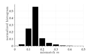
Figure 1: The histogram shows the mismatch distribution for the search template grid of Eq. II.1. The average mismatch is $\langle m\rangle\approx 15\%$.

The parameter space searched by the GC search comprises $\sim 4.4\times 10^{12}$ templates and is split into 10 678 smaller compute jobs, each of which reports the most significant 100 000 candidates, yielding a total of $10^{9}$ candidates to postprocess.

II.2 Comparison to metric grid construction

We can try to estimate the expected mismatch for this template bank using the analytic phase metric [e.g. see Eq.(10) in Wette2008 ] and combining fine- and coarse-grid mismatches (assuming a $\mathbb{Z}_{2}$-like grid structure) by summing them according to Eq.(22) of PrixShaltev:2012 . This naive estimate, however, yields an average mismatch of $\langle m\rangle\approx 0.56$, overestimating the measured value by nearly a factor of 4. One reason for this is the well-known inaccuracy of the metric approximation (particularly the phase metric) for short coherent-search times $\lesssim\mathcal{O}(\text{days})$; see Prix:2006wm ; Wette:2013wza . The second reason stems from the nonlinear effects that start to matter for mismatches $\gtrsim 0.2$ (e.g. see Fig. 10 in Prix:2006wm and Fig. 7 in Wette:2013wza ). A more detailed metric simulation of this template bank, using the average-$\mathcal{F}$ metric (instead of phase metric) and folding in the empirical nonlinear behavior puts the expected average mismatch at $\langle m\rangle\approx 0.2$.

Despite the quantitative discrepancy of the simple phase metric, using it to guide template-bank construction (followed by Monte Carlo testing) would still have been useful. For example, the simplest metric grid construction of a square lattice aiming for an average mismatch of $\sim 0.15$ would result in grid spacings

$$\delta f^{\prime}=\frac{0.37}{T_{\text{seg}}}\,,\;\;\delta\dot{f}^{\prime}_{\text{coarse}}=\frac{2.86}{T_{\text{seg}}^{2}}\,,$$ (5)

and $\delta\dot{f}^{\prime}_{\text{fine}}=\delta\dot{f}^{\prime}_{\text{coarse}}/\gamma$. This corresponds to a $\sim 6\%$ reduction in computing cost compared to the original search, and results in a measured mismatch distribution with an average $\langle m\rangle\approx 0.09$, which corresponds to an improvement in sensitivity. Relaxing those spacings by a factor $1.7$, namely

$$\delta f^{\prime\prime}=\frac{0.63}{T_{\text{seg}}}\,,\;\;\delta\dot{f}^{\prime\prime}_{\text{coarse}}=\frac{4.87}{T_{\text{seg}}^{2}}\,,$$ (6)

and $\delta\dot{f}^{\prime\prime}_{\text{fine}}=\delta\dot{f}^{\prime\prime}_{\text{coarse}}/\gamma$, results in a measured average mismatch of $\langle m\rangle\approx 0.14$, i.e. similar to the original setup, but at a total computing cost reduced by about a factor of $\sim 3.1$. Such large gains are possible here due to the fact that the original search grid of Eq. (II.1) deviates strongly from a square lattice in the metric sense: namely the frequency spacing is about $\sim 80$ times larger in mismatch than the spin-down spacing.

II.3 Data selection

The data used in the GC search come from two of the three initial LIGO detectors, H1 and L1, and were collected at the time of the fifth science run (S5) Abbott2009e . The recorded data were calibrated to produce a GW strain $h(t)$ time series Abbott2009d ; Abbott2009e ; Abadie:2010px which was then broken into $T_{\text{sft}}=1800\,\text{s}$ long stretches, high-pass filtered above 40 Hz, Tukey windowed, and Fourier transformed to form short Fourier transforms (SFTs) of $h(t)$.

Based on constraints stemming from the available computing power, 630 segments, each spanning $T_{\text{seg}}=11.5$ h and generally comprising data from both detectors, were used in the GC search. These data cover a period of 711.4 days which is 98.6% of the total duration of S5. The segments were not completely filled with data from both detectors: the total amount of data (from both detectors) corresponds to 447.1 days, which means an average fill level per detector per segment of $\sim 74\%$.

Different approaches exist for selecting the segments to search from a given data set. We compare different selection criteria by studying the sensitivity of different sets of S5 segments chosen according to the different criteria. We start by creating a set $\mathcal{S}$ comprising all possible segments of fixed length. We then pick 630 nonoverlapping segments from this set according to each criterion.

Set $\mathcal{S}$ is constructed as follows: each segment covers a time $T_{\text{seg}}$ and neighboring segments overlap each other by $T_{\text{seg}}$ - 30 min. The first segment starts at the timestamp of the first SFT of S5. All SFTs that lie entirely within $T_{\text{seg}}$ are assigned to that segment. The second segment starts half an hour later, and so on.

The different sets of segments are constructed as follows: every criterion assigns a different figure of merit to each segment in $\mathcal{S}$. For each criterion we then select the segment with the highest value of the corresponding figure of merit while all overlapping segments are removed from $\mathcal{S}$. From the remaining list, the segment with the next-highest value of the figure of merit is selected, and again all overlapping segments are removed. This is repeated until 630 segments are selected. Since we consider four different criteria this procedure generates four different sets of segments labeled $\mathcal{A}$, $\mathcal{B}$, $\mathcal{C}$ and $\mathcal{D}$. The four different criteria reflect data-selection choices made in past searches, including the one specifically developed for the GC search, which we describe in the following.

The figures of merit are computed at a single fixed frequency. This is possible because the relative performance of the different selection criteria in Gaussian noise does not depend on the actual value of the frequency of the signal. Hence we choose 150 Hz which is in a spectral area that does not contain known disturbances and is representative of the noise in the large majority of the data set.

The first selection criterion is solely based on the fill level of data per segment, as was done in Abbott2009a ; Abbott2009d . The corresponding figure of merit is the number of SFTs in each segment, namely

$$Q_{\mathcal{A}}=N_{\text{seg}}^{\text{SFT}}\,.$$ (7)

The resulting data set is referred to as set $\mathcal{A}$.

The second criterion was used in the first coherent search for CWs from the central object in the supernova remnant Cassiopeia A, where the data were selected based on the noise level of the data in addition to the fill level Wette2010 . The figure of merit is defined as the harmonic sum in each segment of the noise power spectral density at 150 Hz $S_{\mathrm{h}}$ Wette2010 :

$$Q_{\mathcal{B}}=\sum_{k=1}^{N_{\text{seg}}^{\text{SFT}}}\frac{1}{S_{\mathrm{h}}^{k}}\,.$$ (8)

The sum is over all SFTs in the appropriate segment. The resulting data set is referred to as set $\mathcal{B}$.

The third criterion is the first to take into account not only the amount of data in each segment, $N_{\text{seg}}^{\text{SFT}}$, and the quality of the data, expressed in terms of the strain noise $S_{\mathrm{h}}$, but also the quality of the data, expressed in terms of the strain noise $S_{\mathrm{h}}$, and the sensitivity of the detector network to signals from a certain sky position at the time when the data were recorded. This criterion was used for the fully coherent search for CW signals from Scorpius X-1, using 6 h of data from LIGO’s second science run [Eq. 36 in Abbott2007a ]. We define an equivalent figure of merit as

$$Q_{\mathcal{C}}=N_{\text{seg}}^{\text{SFT}}\frac{\sum_{k=1}^{N_{\text{seg}}^{\text{SFT}}}\mathcal{P}^{k}}{\sum_{k=1}^{N_{\text{seg}}^{\text{SFT}}}S_{\mathrm{h}}^{k}},$$ (9)

where $\mathcal{P}^{k}=(F_{+}^{k})^{2}+(F_{\times}^{k})^{2}$ depends on the antenna pattern functions ${F_{+}^{k}}$ and ${F_{\times}^{k}}$ jks , computed at the midtime of each SFT $k$ in the considered segment. The data set that we obtain with this method is referred to as set $\mathcal{C}$.

The fourth criterion is the one used in the GC search. The figure of merit is the average expected detection statistic:

$$Q_{\mathcal{D}}=\overline{\mathrm{E}[2\mathcal{F}]}\,,$$ (10)

where the average denoted by $\overline{\phantom{{}2F{}}}$ is over a signal population with a fixed GW amplitude $h_{0}$ and random polarization parameters ($\cos\iota$ and $\psi$) and where $\mathrm{E}[]$ denotes the expectation value over noise realizations. The resulting data set is referred to as set $\mathcal{D}$.

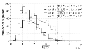
Figure 2: The distributions of the average expected detection statistic over segments, $\overline{\mathrm{E}[2\mathcal{F}]}$. $\overline{\phantom{{}2F{}}}$ denotes the average over a population of signals with a fixed fiducial GW amplitude and random polarization parameters ($\cos\iota$ and $\psi$). The figure shows that a large fraction of the segments in set $\mathcal{D}$ has high $\overline{\mathrm{E}[2\mathcal{F}]}$ values compared to the other sets. We also compare for each set the average value of $\overline{\mathrm{E}[2\mathcal{F}]}$ over the 630 segments, $\langle\overline{\mathrm{E}[2\mathcal{F}]}\rangle$. The higher that number, the more sensitive the data set is.

In order to compare the sensitivity of searches carried out on these different data sets we compute the expected $\mathcal{F}$-statistic value for a signal coming from the GC for the single segments in each of the data sets. Figure 2 shows distributions of the average value of the expected $2\mathcal{F}$ for a population of sources at the GC with a fixed fiducial GW amplitude (and averaged over the polarization parameters $\cos\iota$ and $\psi$) for each segment in sets $\mathcal{A},~{}\mathcal{B},~{}\mathcal{C}$ or $\mathcal{D}$. The integral of each histogram is the number of segments, 630. By construction, sets $\mathcal{A}$, $\mathcal{B}$ and $\mathcal{C}$ cannot be more sensitive than $\mathcal{D}$, but here we quantify the differences: The data set used for the GC search ($\mathcal{D}$) results in an average $2\mathcal{F}$ value (over segments and over a population of signals) that is about 1.5 times higher than that of set $\mathcal{C}$. This translates into a gain of roughly 20%-30% in minimum detectable GW amplitude for set $\mathcal{D}$ with respect to set $\mathcal{C}$. The ratio of the average $2\mathcal{F}$ value between sets $\mathcal{C}$, $\mathcal{B}$ and $\mathcal{A}$ does not exceed 1.1.

An interesting property of the selected data in set $\mathcal{D}$ is that the segments were recorded at times when the detectors had especially favorable orientation with respect to the GC. We can clearly see this from the zoom of Fig. 3 and by comparing the average antenna patterns $\overline{\mathcal{P}(\mathcal{X})}=(1/N^{\mathcal{X}}_{\text{sft}})\sum_{k\in\mathcal{X}}\mathcal{P}_{k}$ for the SFTs $k$ in the data sets $\mathcal{X}=\mathcal{A},\,\mathcal{B},\,\mathcal{C},\,\mathcal{D}$:

$$\overline{\mathcal{P}(\mathcal{A})}=0.38,~{}~{}\overline{\mathcal{P}(\mathcal{B})}=0.37,\overline{\mathcal{P}(\mathcal{C})}=0.50,~{}~{}\overline{\mathcal{P}(\mathcal{D})}=0.56.$$ (11)

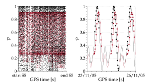
Figure 3: The antenna pattern functions $\mathcal{P}(t_{k})=F_{+}(t_{k})^{2}+F_{\times}(t_{k})^{2}$ at the midtime $t_{k}$ of each SFT of set $\mathcal{D}$ ($k$ indicates the order number of the SFTs and $t_{k}$ is on the x axis). Red color shows the values for H1, black those for L1. The right plot is a zoom of the left plot for a duration of $2.9$ days within the first weeks of S5. As described above, the segments are selected to maximize the expected $2\mathcal{F}$ value which explains the distribution of points along the solid curves. The maximum and minimum values of $\mathcal{P}(t)$ for the Hanford detector, just above 0.9 and just below 0.08, are due to the fact that at the latitude of Hanford ($46^{\circ}17^{\prime}8^{\prime\prime}$) the GC (which has a declination of $-29^{\circ}0^{\prime}28^{\prime\prime}$) can never reach the zenith.

III Postprocessing

III.1 Known-lines cleaning

Terrestrial disturbances affect GW searches in undesired ways. Some disturbances originate from the detectors themselves, like the ac power line harmonics or some mechanical resonances of the apparatus. These (quasi)stationary spectral lines affect the analysis results by generating suspiciously large $\langle 2\mathcal{F}\rangle$ values. Over the last years, knowledge about noise sources has been collected, mostly by searching for correlations between the GW channel of the detector and other auxiliary channels. However, only rarely can those noise sources be mitigated and hence we need to deal with candidates that we suspect are due to disturbances. One of the approaches taken so far consisted of removing candidates that lie within disturbed frequency bands. This can happen both by excluding up front certain frequency bands from the search or by so-called “known-lines cleaning procedures,” two variants of which are discussed below.

III.1.1 The “strict” known-lines cleaning

This cleaning procedure, as it has been used in past all-sky searches (see, for example Aasi:2012fw ), removes all candidates whose value of the detection statistic may have had contributions from data contaminated by known disturbances. In order to determine whether data from frequency bins in a corrupted band have contributed to the detection statistic at a given parameter-space point $\{f,\dot{f}\}$, one has to determine the frequency evolution of the GW signal as observed at the detector during the observation time and see if there is any overlap with the disturbed band. If there is, the candidate from that parameter-space point is not considered. The method actually used is even coarser, since the sky position of the candidate is ignored and the span of the instantaneous frequency is assumed to be the absolute maximum possible over a year, independently of sky position.

Had this method been applied in the GC search, the large spin-down values searched and the regular occurrence of the $1\,\text{Hz}$ harmonics in the S5 data (see Tables VI and VII in Aasi:2012fw ) would have resulted in a huge loss of $\sim 88.6\%$ of all candidates. Such loss is unnecessary as is shown below, and a more relaxed variation on this veto scheme can be used.

III.1.2 The “relaxed” known-lines cleaning

The reason for the above-mentioned loss is twofold: the regular occurrence of 1 Hz harmonics and the large spin-down values searched in the GC search. If a signal has a large spin-down magnitude $|\dot{f}|$, its intrinsic frequency changes rapidly over time and hence it “sweeps” quickly through a large range in frequency. Most templates have spin-down values large enough to enter one of the 1 Hz frequency bands at some point, but they also sweep through the contaminated bands quickly. Consider for instance a contaminated band from the $1\,\text{Hz}$ harmonic at $496\,\text{Hz}$, where the intrinsic width of the $1\,\text{Hz}$ harmonic is maximal and reaches $\Delta f=0.08\,\text{Hz}$. A signal with a spin-down of magnitude $|\dot{f}_{\text{av}}|=5.9\times 10^{-8}\,\text{Hz}/\text{s}$ (the average spin-down value searched in the GC search) sweeps through such a band in $\Delta t=\Delta f/|\dot{f}_{\text{av}}|\simeq 16$ days. Since one data segment spans only about half a day, this means that at most about 32 of the 630 segments contribute data to the detection statistic that may be affected by that artifact, which is only about $\sim 5\%$. This means that only a very small percentage of the data used for the analysis of high spin-down templates is potentially contaminated by a $1\,\text{Hz}$ line.

Based on this, we relax the known-lines cleaning procedure and allow for a certain amount of data to be potentially contaminated by a 1 Hz harmonic. Since the 1 Hz lines are the only artifacts with such a major impact on the number of surviving candidates, the other known spectral lines are still vetoed “strictly.” In the GC search, all candidates with frequency and spin-down values such that no more than $30\%$ of the data used for the analysis of the candidate are potentially contaminated by a 1 Hz line are kept. One could easily argue for a larger threshold than $30\%$, given the negligible impact of the spectral lines. As a measure of safety, all candidates which pass this procedure only due to the relaxation of the line cleaning are labeled. Further investigations can then fold in that information, if necessary.

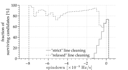
Figure 4: The histograms illustrate the effect of the relaxed known-lines cleaning procedure in the context of the GC search: the black, dashed histogram contains the fraction of candidates that pass the strict known-lines cleaning, the gray, solid histogram shows the fraction of candidates that pass the relaxed known-lines cleaning.

After applying the relaxed known-lines cleaning in the GC search, $83\%$ of the candidates survive. Figure 4 shows the fraction of surviving candidates as a function of their spin-down values for both the strict and the relaxed known-lines cleaning procedure.

III.2 Clustering of candidates

A GW signal that produces a significant value of the detection statistic at the template with the closest parameter match will also produce elevated detection statistic values at templates neighboring the best-match template. This will also happen for a large class of noise artifacts in the data. The clustering procedure groups together candidates around a local maximum, ascribing them to the same physical cause and diminishing the multiplicity of candidates to be considered in the following steps. The clustering is performed based on the putative properties of the signals: assuming a local maximum of the detection statistic due to a signal, the cluster would contain with high probability all the parameter-space points around the peak with values of the detection statistic within at least half of the peak value.

The cluster is constructed as a rectangle in frequency and spin-down. We choose to use the bin size of Eq. II.1 as a measure for the cluster box dimension. The cluster box size is determined by Monte Carlo simulations in which 200 different realizations of CW signals randomly distributed within the ranges given in Table 1 and without noise are created and the data searched. The search grid is randomly mismatched with respect to the signal parameters for every injection. Figure 5a shows the average detection statistic values, each normalized to the value of the maximum for each search, as a function of the frequency and spin-down distance from the location of the maximum. The average is over the 200 searches. Figure 5b shows the standard deviation of the normalized detection statistic averaged in order to determine Fig. 5a.

Figure 6 shows the distribution of the distances in frequency and spin-down bins for average normalized detection statistic values greater than 0.5. Within the neighboring two frequency bins on either sides of the frequency of the maximum, we find $>99\%$ of the templates with average normalized detection statistic values larger than half of the maximum. Of order $95\%$ of the templates that lie within 25 spin-down bins of the spin-down value of the maximum have average normalized detection statistic values larger than half of the maximum. Therefore, we pick the cluster size to be

$$\Delta f_{\text{cluster}}=\pm 2\ \delta f\ \simeq\ 4.8\times 10^{-5}\,\text{Hz}$$

$$\Delta\dot{f}_{\text{cluster}}=\pm 25\ \delta\dot{f}_{\text{fine}}\ \simeq\ 4.5\times 10^{-12}\,\text{Hz}/\text{s}$$ (12)

on either side of the parameter values of the representative candidate.

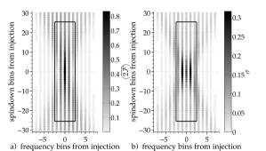
Figure 5: The left plot shows the averaged outcome of 200 searches that were performed on fake data with parameters randomly distributed over the search parameter space. As explained in the text, the detection statistic values are all normalized to the maximum of their respective search and then averaged over the 200 searches in each grid point. The grid points represent distances from the maximum. The right plot gives the standard deviation for each data point of the left plot. The black box denotes the cluster box. All candidates within this box are ascribed to the loudest representative candidate in the center by the clustering procedure.

The clustering procedure is implemented as follows: from the list of all candidates surviving the known-lines cleaning the candidate with the largest $\langle 2\mathcal{F}\rangle$ value is chosen to be the representative for the first cluster. All candidates that lie within the cluster size in frequency and spin-down are associated with this cluster. Those candidates are removed from the list. Among the remaining candidates the one with the largest $\langle 2\mathcal{F}\rangle$ value is identified and taken as the representative of the second cluster. Again, all candidates within the cluster size are associated to that cluster and removed from the list. This procedure is repeated until all candidates have either been chosen as representatives or are associated to a cluster.

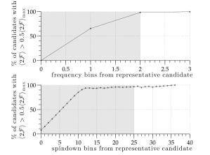
Figure 6: The plot shows the fraction of candidates with $\langle 2\mathcal{F}\rangle$ values larger than half of maximum as a function of distance in frequency (top) and spin-down (bottom), from the maximum. The gray shaded areas denote the boundaries of the cluster box in each dimension.

After applying the clustering procedure to the list of candidates in the context of the GC search, the total number of candidates left for further postprocessing checks is reduced to $\sim 33\%$ of what it was before the clustering procedure.

III.3 The $\mathcal{F}$-statistic consistency veto

The $\mathcal{F}$-statistic consistency veto provides a powerful test of local disturbances by testing for consistency between the multidetector detection-statistic results and the single-detector results. Local disturbances are more likely to affect the data of only one detector and appear more clearly in the single-detector results than in the multidetector results. In contrast, GWs will be better visible when the combined data set is used. The veto which has already been used in past CW searches Aasi:2012fw ; Abbott2009d is simple: for each candidate the single-interferometer values $\langle 2\mathcal{F}\rangle_{\text{H1,L1}}$ are computed. The results are compared with the multi-interferometer $\langle 2\mathcal{F}\rangle$ result. If any of the single-interferometer values is higher than the multi-interferometer value, we conclude that its origin is local and the associated candidate is discarded.

While designing the different steps to be as effective as possible in rejecting disturbances, it is important to make sure that a real GW signal would pass the applied vetoes with high probability. To this end the vetoes are tested on a set of simulated data with signal injections and the false-dismissal rate is estimated. In particular, we create $500$ different data sets consisting of Gaussian noise and signals with parameters randomly distributed within the search parameter space of the GC search. An overview of the injection parameter ranges is given in Table 1. The SFT start times of the test data set equal those of the real data set. Unless stated otherwise, the same procedure is used whenever injection studies are reported throughout the paper. The data are searched with the same template grid as used in the original search, in a small region around the signal parameters, and the maximum from that search is taken as the resulting candidate.

Parameter		Range
Signal strength		$h_{0}^{\text{injected}}=h_{0}^{90\%}(f)$ of the GC search
Sky position [rad]		$\lvert\Delta\alpha\rvert+\lvert\Delta\delta\rvert\leq 10^{-3}\,\text{rad}$
		with $\Delta\{\alpha,\delta\}=\{\alpha,\delta\}_{\text{inj}}-\{\alpha,\delta\}_{\text{GC}}$
Frequency [Hz]		$150\,\text{Hz}\leq f\leq 152\,\text{Hz}$
Spin-down [Hz/s]		$-f/200\ \text{yr}\leq\dot{f}\leq 0$
Polarization angle		$0\leq\psi\leq 2\pi$
Initial phase constant		$0\leq\phi_{0}\leq 2\pi$
Inclination angle		$-1\leq\cos\iota\leq 1$

Table 1: Parameters of the fake signal injections performed for the false-dismissal studies. Unless explicitly stated in the text, $500$ signals are injected into fake Gaussian noise.

The $\mathcal{F}$-statistic consistency veto is found to be very safe against false-dismissals: none of the $500$ signal injections is vetoed, which implies a false-dismissal rate of $\lesssim 0.2\%$ for the tested population of signals.

In the GC search, this veto removes $12\%$ of the tested candidates.

III.4 The significance threshold

At some point in most CW searches, a significance threshold is established below which candidates are not considered. This threshold limits the ultimate sensitivity of the search. Where one sets this threshold depends on the available resources for veto and follow-up studies. If no resources are available beyond the ones used for the main search, this detection threshold will be based solely on the results from that first search. If there are computing resources available to devote to follow-up studies, the threshold should be the lowest such that candidates at that threshold level would not be falsely discarded by the next stage and such that the follow-up of all resulting candidates is feasible. From these considerations follows a significance threshold of $\langle 2\mathcal{F}\rangle\geq 4.77$ for the GC search myobspaper . This reduces the number of candidates to follow up to a number of 27 607 which, after the next veto and excluding the candidates that we can associate to fake signals present in the data stream for validation purposes, becomes manageable for a sensitive enough follow-up. In the absence of surviving candidates at any threshold one can always set upper limits based on the loudest surviving candidate below the threshold, assuming that it is due to a putative signal.

III.5 The permanence veto

Until now we have not required the searched GW signals to have any specific characteristics other than having consistent properties among the two detectors used for the analysis. To further reduce the number of candidates to follow-up (and hence attain a higher sensitivity) we now restrict our search to strictly continuous signals and use their assumed permanence during the observation time to define the next veto. We stress that GW signals such as strong transient GW signals prixetal2011:_transientCW ; 2011PhRvD..83h3004T lasting a few days or weeks which might have survived up to this point would be dismissed by this veto. With this step we trade breadth of search in favor of depth.

In a stack-slide search the detection statistic $\langle 2\mathcal{F}\rangle$ is the average of the $2\mathcal{F}$ values computed for each of the segments and we expect that the SNR of a signal to be comparable in every segment. However, in the final result the relative contribution of the different segments to this average is “invisible.” This information is important, though, because a strong-enough disturbance can cause a large $\langle 2\mathcal{F}\rangle$ value, even though only a few segments effectively contribute to it. The following veto aims to uncover behavior of this type and discard the associated candidates.

In the context of the GC search we found that in most cases it is only a single segment which contributes a large $\langle 2\mathcal{F}\rangle$ value. This observation inspired the definition of the simple veto that was used: for each candidate the values of $2\mathcal{F}$ for each of the $630$ data segments are determined. The highest value is removed and a new average over the remaining $629$ segments is computed. If this value is below the significance threshold (see Sec. III.4), the candidate is vetoed.

The permanence veto was highly effective in the GC search where it ruled out about 96% of the candidates from the previous stage. At the same time it is very safe, with a false-dismissal rate of only $\simeq 0.6\%$ for the given signal population (see Table 1). Figure 7 shows the distribution of the $\langle 2\mathcal{F}\rangle$ values before and after removing the loudest segment contribution. One can clearly see that removing the loudest contribution shifts the distribution from above to below the threshold for most of the candidates that were tested with this veto in the context of the GC search (7a), but does not change the distribution when applied to a set of signal injections (7b).

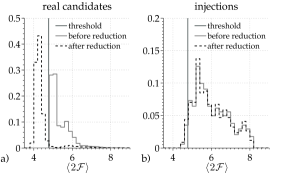
Figure 7: The distribution of $\langle 2\mathcal{F}\rangle$ values before and after removing the contribution from the loudest among the different segments (a) for real candidates and (b) for a set of signal injections. Removing the contribution of the loudest segment shifts the distribution of $\langle 2\mathcal{F}\rangle$ values from just above to below the significance threshold at $\langle 2\mathcal{F}\rangle=4.77$ (vertical line). This clearly shows that most candidates have significant $\langle 2\mathcal{F}\rangle$ values only due to a single segment that contributes an extremely large $2\mathcal{F}$ value. The distribution of $\langle 2\mathcal{F}\rangle$ values from a set of continuous signal injections does not change: the contribution of all segments to the average value is comparable.

III.6 Coherent follow-up search and veto

The semicoherent technique used in the GC search is a powerful way to search a large parameter space, but this benefit comes at the cost of reduced sensitivity: a semicoherent analysis does not recover weak signals with the same significance as a coherent search technique could do on the same data set and with comparable mismatch distributions, and it does not estimate the parameters of a signal as precisely as a coherent analysis would. We recall that the advantage of using semicoherent techniques is that they allow the probing of large parameter-space volumes, over large data sets with realistic amounts of computing power.

A coherent follow-up search can now be used on a subset of the original parameter space identified as significant by the previous stages (see Fig. 8). By appropriately choosing the coherent observation time, we ensure that this search rules out with high confidence candidate signals that fall short of a projected detection statistic value.

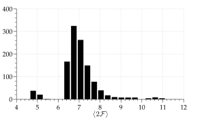
Figure 8: The histogram shows the distribution of the $\langle 2\mathcal{F}\rangle$ values of the 1 138 candidates that are investigated in the follow-up search. All candidates with values larger than 6 can be ascribed to a pulsar signal hardware injection that was performed during S5.

The process of determining the optimal coherent observation time, under constraints on computing power and on the precision of the candidate signals’ parameters, is iterative. In the GC search a setup was determined that was able to coherently follow up the remaining 1 138 candidates, having allocated on average 10 h of computing time for each candidate. The chosen data set spanned $T_{\text{coh}}=90$ days and yielded a moderate computing cost of the order of a day on several hundred compute nodes of the ATLAS cluster.

In the following we detail a single-stage follow-up procedure with this coherent observation time, illustrate the condition used to test the candidates after the follow-up and demonstrate its effectiveness.

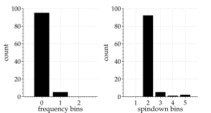
Figure 9: The two histograms show the distances (absolute value) between the parameters of the loudest template and the parameters of the injected signal measured in frequency and spin-down bins of the initial search [i.e. with the spacing of Eq. II.1]. The counts refer to values of the distances between the right and left edges of each bin.

III.6.1 The search volume

The parameters of the candidates are only approximations to the real signal’s parameters. In order to establish the parameter-space region that we need to search around each candidate in the follow-up search, we have studied the distribution of distances between the injection parameters and the recovered parameters for a population of fake signals designed to simulate the outcome of the original search.

In particular, we have performed a Monte Carlo study over $100$ fake signals with parameters distributed as described in Table 1 without noise. The data are searched with the template grid resolution of the GC search in a box of $50$ frequency bins and $100$ spin-down bins, placed around each injection. Then the distance in frequency and spin-down between the loudest candidate and the injection is evaluated. The distributions of these distances are shown in the histograms in Fig. 9. In all cases, the distance is smaller or equal to two frequency and five spin-down bins. Consequently, the frequency and spin-down ranges for the coherent follow-up search are set to be:

$$\Delta f=\pm 2\ \delta f\rightarrow 1.2\times 10^{-4}\,\text{Hz}$$

$$\Delta\dot{f}=\pm 5\ \delta\dot{f}_{\text{fine}}\rightarrow 2.0\times 10^{-12}\,\text{Hz}/\text{s}.$$ (13)

In order to keep the computational cost of the follow-up stage within the set bounds we restrict the search sky region to a distance of 3 pc around the GC.

III.6.2 The grid spacings

The frequency-spin-down region in parameter space around each candidate defined by Eq. III.6.1 is covered by a template grid refined with respect to the original one of Eq. II.1, as follows:

$$\delta f_{\text{coh}}=(2\ T_{\text{coh}})^{-1}=6.4\times 10^{-8}\,\text{Hz}$$

$$\delta\dot{f}_{\text{coh}}=(2\ T_{\text{coh}}^{2})^{-1}=8.3\times 10^{-15}\,\text{Hz}/\text{s}.$$ (14)

The sky region to be searched is covered by a $6\,\times\,6$ rectangular grid in right ascension and declination, across $7.2\times 10^{-4}$ rad in each dimension.

With all these choices the resulting mismatch distribution over 1 000 trials in Gaussian noise is shown in Fig. 10. It has an average of $\langle m_{\text{coh}}\rangle=1\%$ and reaches 4.7% in $\lesssim 1\%$ of the cases.

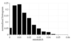
Figure 10: This histogram shows the mismatch distribution of the follow-up search. The average value is $\langle m_{\text{coh}}\rangle=1\%$. Only in a small fraction of cases ($\lesssim 1\%$) can the mismatch be as high as 4.7%.

III.6.3 The expected highest $2\mathcal{F}$ in Gaussian noise

The follow-up of the region of parameter space around each candidate defined in Eq. III.6.1 and covered by the grids defined in Eq. III.6.2 results in a total of $N_{\text{coh}}=N_{f}\times N_{\dot{f}}\times N_{\text{sky}}\sim 16\times 10^{6}$ templates. The expected largest $2\mathcal{F}$ value for Gaussian noise and for $N_{\text{coh}}$ independent trials is $E[2\mathcal{F}^{\ast}_{\text{coh, G}}]=40$ myobspaper with a standard deviation $\sigma_{G}=4$. However, this is an overestimate since the templates in our grids are not all independent of one another. We estimate the effective number of independent templates through the actual measured distribution. This is obtained by a Monte Carlo study in which $1\,000$ different realizations of Gaussian noise are analyzed, using the search box and the template setup of the coherent follow-up search. The loudest detection statistic value from each search is recorded. Figure 11 shows the distribution of such largest $2\mathcal{F}^{\ast}_{\text{coh,G}}$ values. The measured mean value is $35$ and the measured standard deviation is $3$. We superimpose the analytic expression for the expectation value [see Wette2010 , Eq. 7] for an effective number of templates $N_{\text{eff}}\sim 0.1\ N_{\text{coh}}$. The analytic estimate with $N_{\text{eff}}$ has a mean value of 36 and a standard deviation of 3.

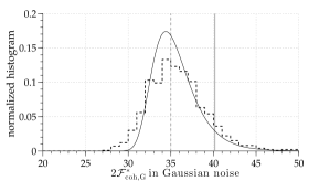
Figure 11: This histogram shows the distribution of the maximum $2\mathcal{F}^{\ast}_{\text{coh,G}}$ resulting from a coherent follow-up search. A thousand searches with grids defined by Eq. III.6.2 were performed, with different realizations of pure Gaussian noise (black dashed line). The mean value measured on this distribution is $35\pm 3$ (dashed gray line). Based on the total number of templates $N_{\text{coh}}$, the predicted mean is $E[2\mathcal{F}^{\ast}_{\text{coh, G}}]=40\pm 4$ (solid gray line). From the simulation data the number of effective independent templates can be estimated to $N_{\text{eff}}\sim 0.1\ N_{\text{coh}}$ (black line). The solid black line is the estimated probability density function for the maximum under the assumption of $N_{\text{eff}}$ independent templates.

III.6.4 The expected detection statistic for signals

In the presence of a signal the coherent detection statistic $2\mathcal{F}$ follows a $\chi^{2}$ distribution with four degrees of freedom and a noncentrality parameter $\rho^{2}$ which depends on the noise floor and on the signal amplitude parameters and scales linearly with the coherent observation time. The expected value of $2\mathcal{F}$ is $\mathrm{E}[2\mathcal{F}]=4+\rho^{2}$.

For every candidate the $\langle 2\mathcal{F}\rangle$ value can be expressed in terms of the $\langle\rho^{2}_{\text{cand}}\rangle$ associated with that candidate: $\langle\rho^{2}_{\text{cand}}\rangle=\langle 2\mathcal{F}\rangle_{\text{cand}}-4$. Based on $\langle\rho^{2}_{\text{cand}}\rangle$ we then estimate the expected detection statistic of a coherent follow-up with $T_{\text{coh}}$ data simply as

$$2\mathcal{F}^{\text{cand}}_{\text{coh}}=\kappa\left(\langle\rho^{2}_{\text{cand}}\rangle\frac{T_{\text{coh}}}{T_{\text{seg}}}\right)+4,$$ (15)

where $\kappa$ is the ratio between the sum over the antenna pattern functions for each SFT $i$ used by the coherent follow-up search and the SFTs $j$ of the original search, respectively:

$$\kappa=\frac{\sum_{i}\left(F_{+}^{2}+F_{\times}^{2}\right)_{i,\text{coh}}}{\sum_{j}\left(F_{+}^{2}+F_{\times}^{2}\right)_{j,\text{orig}}}.$$ (16)

This antenna pattern correction $\kappa$ is important, because it accounts for intrinsic differences in sensitivity to a source at the GC between the data set of the original search and the data set used for the follow-up. For the original search, a data-selection procedure was used to construct the segments at times when the detectors were particularly sensitive to the GC. In contrast, $T_{\text{coh}}$ spans many weeks and also comprises data that were recorded when the orientation between the detector and the GC was less favorable. For this reason, a simple extrapolation of the $\langle 2\mathcal{F}\rangle_{\text{cand}}$ values from the original search to estimate the result of the follow-up search without such a correction, folding in implicitly the assumption that the antenna pattern values for the data of the original search data set are equivalent to those of the follow-up search data set, would result in significantly wrong predictions.

The chosen data set of the follow-up search comprised data from the H1 and L1 detectors and spanned 90 days in the time between February 1, 2007, at 15:02 GMT and May 2, 2007, at 15:02 GMT. It contained a total of $6\,522$ SFTs ($3\,489$ from H1 and $3\,033$ from L1) which is an average of $67.9$ days from each detector (fill level of 75.5%). The antenna pattern correction for this data set and the one used in the original search can be computed with Eq. 16 and results in $\kappa=0.68$. The fact that $\kappa<1$ shows the effect of having chosen data segments for the original search that were recorded at times with favorable orientation between the detectors and the GC, whereas in a contiguous data stretch as long as 90 days the antenna patterns average out.

III.6.5 The $\mathcal{R}$ veto

The expected $2\mathcal{F}^{\text{cand}}_{\text{coh}}$ for each candidate is computed. A follow-up search is performed as specified in the previous sections and the resulting highest value $2\mathcal{F}^{\ast}_{\text{coh}}$ is identified. We define the ratio

$$\mathcal{R}:=\frac{2\mathcal{F}^{\ast}_{\text{coh}}}{2\mathcal{F}^{\text{cand}}_{\text{coh}}}.$$ (17)

A threshold $\mathcal{R}_{\text{thr}}$ is set on $\mathcal{R}$ and candidates with $\mathcal{R}<\mathcal{R}_{\text{thr}}$ are ruled out as GW candidates: their measured detection statistic value after the follow-up falls short of the predictions. The threshold is obtained empirically with a Monte Carlo study with $1\,000$ signal injections in Gaussian noise. The signal parameters are uniformly randomly distributed within the ranges given in Table 1. Two separate data sets are created for this study: one that matches the original data set (in terms of SFT start times) and one that matches the $90$-days coherent data set. Figure 12 shows the distribution of the corresponding values of $\mathcal{R}$. The peak of the distribution of $\mathcal{R}$ is slightly above 1. This means that we slightly underestimate the outcome of the coherent follow-up search.

We place the threshold at $\mathcal{R}_{\text{thr}}=0.5$. The plot shows that $\mathcal{R}<0.5$ for only four out of the $1\,000$ injected signals. This implies a false-dismissal rate of $\sim 0.4\%$.

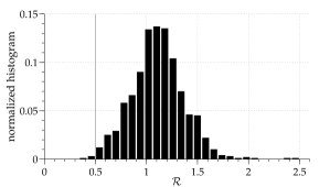
Figure 12: False dismissal: The plot shows the distribution of $\mathcal{R}$ for $1\,000$ different realizations of CW signals in Gaussian noise with parameters randomly distributed within the search parameter space. The threshold is set to $\mathcal{R}_{\text{thr}}=0.5$ (gray line). Only four of the $1\,000$ signals have $\mathcal{R}<\mathcal{R}_{\text{thr}}$, implying a false-dismissal rate of $0.4\%$.

Although a candidate that would pass the coherent follow-up $\mathcal{R}$ veto would still need to undergo further checks to be confirmed as a GW signal, it would all the same be exciting. To estimate the chance of a false-alarm event in Gaussian noise, a Monte Carlo study is performed on purely Gaussian data. We assume that the candidates have an original $\langle 2\mathcal{F}\rangle$ value at the significance threshold $\langle 2\mathcal{F}\rangle=4.77$ which translates into $\rho^{2}_{\text{cand}}\approx 0.77$. Such a candidate represents the lowest $\langle 2\mathcal{F}\rangle$ values considered in this search and will thus yield the highest false alarm. The expected $2\mathcal{F}^{0.77}_{\text{coh}}$ value for the coherent follow-up search for such candidates is $2\mathcal{F}^{0.77}_{\text{coh}}=105.83$. Now, $1\,000$ different realizations of pure Gaussian noise are created and searched with the coherent follow-up search setup. In each of these the loudest candidate is identified and $\mathcal{R}$ is computed. Figure 13 shows the resulting distribution. None of the values exceeds the threshold, yielding a Gaussian false-alarm rate for this veto of $\leq 0.1\%$. Of course the actual false-alarm rate would need to be measured on noise that is a more faithful representation of the actual data rather than simple Gaussian noise. This is not trivial because one would need to characterize the coherence properties of very weak disturbances in the data, which has never been done.

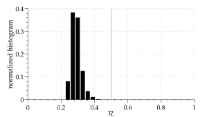
Figure 13: False alarm: The least significant candidates that are considered in the follow-up have $2\mathcal{F}$ values at the significance threshold. Those candidates are expected to result in a value of $2\mathcal{F}^{0.77}_{\text{coh}}=105.83$ in the follow-up search if they are due to a CW. This plot shows the distribution of $\mathcal{R}$ values resulting from a follow-up search on 1 000 different realizations of Gaussian noise. None of the candidates satisfied the condition $2\mathcal{F}^{\ast}_{\text{coh}}>52.9$, which implies a Gaussian false-alarm rate of $\leq 0.1\%$.

Six of the 1 138 tested candidates pass this veto in the GC search, and all of them can be ascribed to a hardware injection performed during S5 hardwareinjections ; beritthesis .

IV Upper limits

No GW search to date has yet resulted in a direct detection. For CW searches a null result is typically used to place upper limits on the amplitude of the signals with parameters covered by the search. In wide parameter-space searches these are typically standard frequentist upper limits (as they were reported in Abbott:2003yq ; Abbott2005a ; Abbott2007a ; Abbott2008a ; Abbott2009c ; Aasi:2012fw ) based on the so-called “loudest event.” In most searches they are derived through intensive Monte Carlo procedures. Only one search has used a numerical estimation procedure to obtain upper-limit values Wette2008 . In the GC search a new, very cost-effective analytic procedure was used which we describe here.

IV.1 The constant-$\eta$ sets

Generally, the search frequency band is divided into smaller sets and a separate upper limit is derived for a population of signals with frequencies within each of these. The partitioning of the parameter space can be done in different ways, with different advantages and disadvantages. Past searches have often divided the parameter space into equally sized frequency bands. For example, the Einstein@Home all-sky searches have divided the frequency band into $0.5$ Hz-wide subbands, e.g. Aasi:2012fw . For a search like the GC search, where the spin-down range grows with frequency, such an approach would lead to significantly larger portions of parameter space for sets at higher frequencies. Therefore, a slightly different approach is followed which divides the parameter space into sets containing an approximately constant number of templates. The main advantage of this approach is the approximately constant false-alarm rate over all sets. The total number of templates $N$ is divided into $3\,000$ sets of $\sim\eta$ templates by subdividing the total frequency range covered by the search into smaller subbands. This results in sets small enough that the noise spectrum of the detectors is about constant over the frequency band of each set. The number of templates in a set that spans a range $\Delta f=f_{\text{max}}-f_{\text{min}}$ in frequency and $\Delta\dot{f}=\dot{f}_{\text{max}}-\dot{f}_{\text{min}}$ in spin-down is calculated with

$$\eta =\eta_{f}\times\eta_{\dot{f}}=\frac{\Delta f}{\delta f}\times\frac{\Delta\dot{f}}{\delta\dot{f}}$$ (18)

where the spacings are given in Eq. II.1. Hence, for a given minimum frequency $f_{\text{min}}$, the maximum frequency $f_{\text{max}}$ associated with a set is

$$f_{\text{max}} =\frac{f_{\text{min}}}{2}+\sqrt{\left(\frac{-f_{\text{min}}}{2}\right)^{2}+\eta\ (200\ \text{yr})\ \delta f\ \delta\dot{f}}.$$ (19)

The total number of templates searched in the GC search, $N\simeq 4.4\times 10^{12}$, is in this way divided into the $3\,000$ sets, each containing $\eta\simeq 1.5\times 10^{9}$ templates.

Because of known detector artifacts in the data (see Sec. III.1), not each of these sets is assigned an upper-limit value. Some sets entirely comprise frequency bands excluded from the postprocessing by the known-lines cleaning procedure. We cannot make a statement about the existence of a GW signal in such sets and, hence, no upper-limit value is assigned to those sets. Other sets are only partially affected by the known artifacts and an upper-limit value can still be assigned on the considered part of the parameter space. However, in order to keep the parameter-space volume associated with each set about constant, upper-limit values are assigned only on sets with a relatively low fraction of the excluded parameter space, as will be explained below.

Figure 14 gives an overview of the excluded parameter space per set. Each black data point denotes the amount of excluded parameter space for one set. The additional red lines mark the known spectral artifacts of the detector that are vetoed strictly (the 1 Hz lines are not shown). The $60$ Hz power lines are clearly visible, as well as, for example, the calibration line at $393.1$ Hz (compare Tables VI and VII in Aasi:2012fw ). The effect of the presence of the $1\,\text{Hz}$ harmonics is visible throughout the whole frequency range.

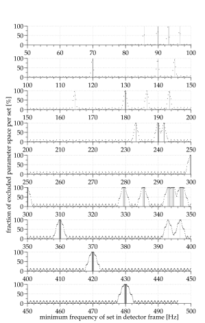
Figure 14: Here we show the percentage of excluded parameter space per upper-limit set as a function of frequency. The gray vertical lines denote the frequencies that host known detector artifacts and which are cleaned strictly. The 1 Hz lines are not shown. The periodical variations of the excluded parameter space are due to the $1\,\text{Hz}$ harmonics. We remind the reader that the searched frequency band starts at $78$ Hz and ends at $496$ Hz.

An upper-limit value is assigned to all sets for which the excluded parameter space is not more than $13\%$ of the total. Figure 15 shows the cumulative distribution of the excluded parameter space of the $3\,000$ sets. The shape of the distribution clearly suggests picking the threshold at $13\%$, which keeps the maximum number of segments while minimizing the excluded parameter space per segment. As a result, an upper-limit value is placed on $2\,549$ sets.

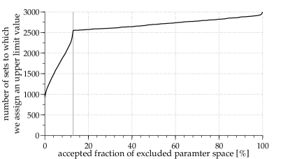
Figure 15: The cumulative distribution of the excluded parameter space per set (black line). The distribution shows a steep increase towards the $13\%$ threshold (gray line). After reaching that threshold, the distribution has a shallow knee up to the $100\%$ loss. As explained in the text, the shape of this distribution simplifies the choice of the threshold.

IV.2 The CW loudest-candidate upper limit

The standard frequentist upper limit is the intrinsic gravitational-wave amplitude such that a high fraction (90% or 95%) of the population of signals being searched, at that amplitude, would have yielded a value of the detection statistic higher than the highest one that was produced by the search (including any postprocessing). The direct way to determine the upper limit value consists of injecting a certain number [$\mathcal{O}(100)$] of signals into the original data set used for the search. The injected signals have parameters randomly distributed within the searched parameter space. All signals are injected at fixed amplitude $h_{0}$. A small region around the injections in frequency and spin-down (and for the all-sky searches also in sky) is analyzed and the loudest candidate is identified. This candidate then undergoes the complete postprocessing pipeline. If it survives all vetoes, and if its $\langle 2\mathcal{F}\rangle$ value exceeds the $\langle 2\mathcal{F}\rangle$ of the most significant surviving candidate from the search, then such an injection is counted as recovered. The fraction of all recovered injections to the total number of injections gives the confidence value $C(h_{0})$. The $h_{0}$ value associated with, say, $90\%$ confidence is $h_{0}^{90\%}$. If a signal of that strength had been present in the data, $90\%$ of the possible signal realizations would have resulted in a more significant candidate than the loudest that was measured. Thus, the presence of a signal of strength $h_{0}^{90\%}$ or louder in the data set is excluded and $h_{0}^{90\%}$ is the $90\%$ confidence upper-limit value on the GW amplitude.

A different $h_{0}^{90\%}$ can be assigned to different portions of the searched parameter space. It will depend on the loudest candidate from that portion of parameter space, on the noise in that spectral region and on the extent of the parameter space. In general, in order to derive the upper limit for each portion of parameter space, several injection sets at different $h_{0}$ values have to be carried out in order to bracket the desired confidence level. Ultimately, an interpolation can be utilized to estimate $h_{0}^{C}$. This standard approach is extremely time consuming because it requires the production and search of several hundred fake data sets for each portion of parameter space on which an upper limit is placed.

IV.3 Semianalytic upper limits

The basic idea is that it is not necessary to sample the different $h_{0}$ values with different realizations of the noise and polarization parameters. Instead, the same noise and signal realizations can be reused for different $h_{0}$ values to sample at virtually no cost the $C(h_{0})$ function and find the upper-limit value at the desired confidence level.

The relation between the measured $\langle 2\mathcal{F}\rangle$ value and the injection strength $h_{0}$ can to good approximation be described by the following relation:

$$\langle 2\mathcal{F}\rangle\simeq\langle\mathcal{N}\rangle+\langle\mathcal{G}\rangle h_{0}^{2},$$ (20)

where $\langle\mathcal{N}\rangle$ represents the average contribution of the noise to the detection statistic value for a given putative signal and $\langle\mathcal{G}\rangle$ is proportional to the average contribution of the signal and depends on the signal parameters, on the timestamps of the data and on the noise-floor level. We fix the parameters that define a signal and we obtain $\langle\mathcal{N}\rangle$ and $\langle\mathcal{G}\rangle$ from the $\langle 2\mathcal{F}\rangle$ values measured by injecting two signals with a different $h_{0}$ value, keeping all other parameters fixed. With this information it is possible to estimate $\langle 2\mathcal{F}\rangle$ for any value of $h_{0}$ for that particular combination of signal parameters and data set. With two sets of $N_{t}$ injections and searches we produce $N_{t}$ $\{\langle\mathcal{N}\rangle,\langle\mathcal{G}\rangle\}$ couples, corresponding to $N_{t}$ signals. We use these $\{\langle\mathcal{N}\rangle,\langle\mathcal{G}\rangle\}$ couples to predict $N_{t}$ values of $\langle 2\mathcal{F}\rangle$ for any $h_{0}$ with Eq. 20. From these the confidence is immediately estimated by simply counting how many exceed the loudest measured one, without further injection-and-search studies.

This semianalytic upper-limit procedure requires only two cycles through the injection-and-search procedure per signal, corresponding to two different signal strengths, namely $5\times 10^{-25}$ and $7\times 10^{-25}$ for the GC search. With $2\,549$ upper-limit sets, each requiring $N_{t}=100$ signals, this results in $509\,800$ injections. In some especially noisy sets, more than $100$ injections are performed amounting to a total of $796\,400$ injections. Each job needs about 20 min to create and search the data. Assuming $\sim 1\,000$ jobs running in parallel on the ATLAS compute cluster, the whole procedure takes a few days up to a week. This is significantly less than the time needed by the standard approach (days as opposed to weeks).

The main advantage of our method is that the injections can be made with arbitrary signal amplitudes, while the standard approach requires an educated guess of $h_{0}$ to start with. The standard injection-and-search procedure is then repeated for different $h_{0}$ values until the 90% confidence upper limit-value is found. In principle, once the first $h_{0}^{90\%}$ value is found, one can rescale it by the noise level to estimate the $h_{0}$ upper limit of neighboring sets. But these values are oftentimes not correct, because of noise fluctuations in the data within one set. Experience has shown that at least five to ten different $h_{0}$ values need to be explored for each band, resulting in a computational effort several times larger than that of our semianalytic procedure.

To estimate the uncertainty on the upper-limit values we use a linear approximation to the curve $C(h_{0})$ in the neighborhood of $h_{0}^{90\%}$. Figure 16 shows $C(h_{0})$ in that region for a set at about $150$ Hz. The $1\sigma$ uncertainty in $C(h_{0})$ based on the binomial distribution for $100$ trials with single-trial probability of success $90\%$, is $3\%$. As illustrated in Fig. 16, this corresponds to an uncertainty of $\lesssim 5\%$ on $h_{0}^{90\%}$.

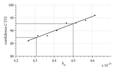
Figure 16: The plot shows $C(h_{0})$ for different $h_{0}$ values for one example set. By fitting a straight line to the data points in a small enough region around the $90\%$ confidence value the $3\%$ error on the confidence can be translated into an uncertainty of $\lesssim 5\%$ on $h_{0}^{90\%}$.

The choice of $N_{t}=100$ allows significant savings with respect to the standard upper-limit procedure and also yields statistical uncertainties which are acceptable ($5\%$ is less than the typical uncertainty in the calibration amplitude which is typically $\sim 10\%$). However, one may still wonder whether 100 signals are a representative sample of the signal population in the parameter-space volume that the upper limit refers to. To prove this we have compared the results of the semianalytic upper-limit procedure for different numbers of trials from $N_{t}=10$ to $N_{t}=1\,000$. The results of this study confirm the 5% error on $h_{0}^{90\%}$. A larger number of trials leads to a reduced uncertainty, like $\sim 2\%$ for $N_{t}=200$ and $<1\%$ for $N_{t}=1\,000$.

Finally, we validate the results of the semianalytic procedure using the standard injection-and-search procedure on a sample of sets. For this we inject 100 signals corresponding to the signal population described in Table 1 into the original search data set. The data are analyzed in a small template grid around the injection (a subset of the original grid) and the loudest candidate is identified. The confidence value is obtained by counting in what fraction of the 100 trials this candidate has a higher $\langle 2\mathcal{F}\rangle$ value than the loudest remaining candidate in that set. Table 2 shows the results for ten different, randomly chosen sets. In all but two cases the measured confidence lies within $1\sigma$ statistical uncertainty value based on 100 trials. In the other two sets the confidence is larger than $90\%$ plus one standard deviation.

Set ID	$~{}f_{\text{min}}^{\text{set}}$[Hz]	$h_{0}^{90\%}[\times 10^{-25}]~{}$	Threshold	$~{}~{}C(h_{0}^{90\%})$[%]
$57$	$103.12$	$5.85$	$4.7523$	$93$
$254$	$162.42$	$3.67$	$4.7098$	$92$
$363$	$187.34$	$3.80$	$4.7098$	$88$
$631$	$237.77$	$4.50$	$4.7394$	$92$
$1025$	$296.74$	$5.52$	$4.7497$	$90$
$1586$	$364.61$	$7.13$	$4.7446$	$90$
$1672$	$373.93$	$6.75$	$4.6984$	$90$
$2302$	$436.16$	$7.77$	$4.7218$	$93$
$2695$	$470.83$	$8.49$	$4.7303$	$94$
$2972$	$493.81$	$11.8$	$4.7170$	$100$

Table 2: Validation of the $h_{0}^{90\%}$ values obtained with the semianalytic procedure for ten sample sets. For each set $100$ GW signals have been injected at the $h_{0}^{90\%}$ level into the search data set. The confidence is the fraction of these injections that was recovered with a higher $\langle 2\mathcal{F}\rangle$ value than that of the loudest surviving candidate of that set.

We note that in the upper-limit procedure we do not subject the injections to any of the postprocessing vetoes (including the follow-up) that we apply to the search. This is because of the very low false-dismissal rate of these vetoes. In $98.1\%$ of all cases in which a signal candidate is not recovered, it is because the candidate fails the comparison with the loudest surviving candidate from the search in that set. Only in $0.2\%$ of the cases is it the $\mathcal{F}$-statistic consistency veto that discards the candidate and in $1.7\%$ the candidate is lost at the permanence veto step. This systematic loss of detection efficiency was neglected in the GC search and it would have resulted in a 3% increase in the upper-limit values, as can be seen from Fig. 16.

V Second-order spin-down

All methods described in the previous sections have been assessed on a population of signals without second-order spin-down. However, if the observation time is of the order of years, the second-order spin-down has an impact in the incoherent combination of the single-segment results. The minimum second-order spin-down signal that is necessary to move the signal by a frequency bin $\delta f$ within an observation time $T_{\text{obs}}$ is

$$\ddot{f}_{\text{min}}=\frac{\delta f}{T_{\text{obs}}^{2}}.$$ (21)

In case of the GC search this value is $\sim 6\times 10^{-21}\,\text{Hz}/\text{s}^{2}$.

To quantify the false-dismissal for signals with second-order spin-down we perform an injection-and-search Monte Carlo study where we inject signals with a second-order spin-down and search for them and perform postprocessing as described above, namely without taking account of a second-order spin-down. A set of $500$ signal injections is created with the parameters given in Table 1 and with an additional second-order spin-down value in the range $0\leq\ddot{f}\leq n\dot{f}^{2}/f$ Palomba:1999su with a braking index of $n=5$ Wette2010 . Since the second-order spin-down values are drawn from a uniform random distribution, most of them fall in the higher range ($\ddot{f}\sim 10^{-17}\,\text{Hz}/\text{s}^{2}$) and this study is representative of the worst case (high second-order spin-down) scenario. The data are analyzed using the original template setup of the corresponding job of the search and the highest $\langle 2\mathcal{F}\rangle$ value within a region as large as the cluster size around the injection is recovered. The 36 signals would not have been recovered by the original search because they would not have been included in the top 100 000 that were recorded. Of the remaining $464$ candidates from the injections 458 survive the $\mathcal{F}$-statistic consistency veto, which implies a false-dismissal rate of $\sim 1.3\%$. The next step is the selection of the most significant subset with a significance threshold at $\langle 2\mathcal{F}\rangle\geq 4.77$. A total of 322 ($\sim 70.3\%$) of the signals are above this threshold. Then, the permanence veto is applied and nine signals are lost, corresponding to a false-dismissal rate of $\sim 2.8\%$. Overall, the postprocessing steps up to the coherent follow-up amount to a loss of signals of about 37%, mostly due to the application of the significance threshold. However, as mentioned above, this loss is the result of a worst case study. We find empirically that at $\ddot{f}\leq 5\times 10^{-20}\,\text{Hz}/\text{s}^{2}$ the additional second-order spin-down component does not change the false-dismissal rates and upper-limit results reported above (for the targeted signal population).

Obtaining the false-dismissal rates for a variety of different second-order spin-down values for the $\mathcal{R}$ veto in the coherent follow-up search is computationally very demanding. Therefore, we restrict our study to a few second-order spin-down values. The false-dismissal remains very low for second-order spin-down signals with values lower or equal to $5\times 10^{-20}\,\text{Hz}/\text{s}^{2}$. In a study over $1\,000$ injections no candidate was lost, hence, the false-dismissal rate is $\leq 0.1\%$. In contrast, the false-dismissal rate for a signal population with second-order spin-down values of $4\times 10^{-17}\,\text{Hz}/\text{s}^{2}\leq\ddot{f}\leq 5\times 10^{-17}\,\text{Hz}/\text{s}^{2}$ is about $82\%$. Based on this, we expect our search to be significantly less sensitive for signals with a second order spin down larger than $5\times 10^{-20}\,\text{Hz}/\text{s}^{2}$. We find that the 90%-confidence upper limit values for a population with second-order spin-down values of order $\sim 10^{-17}\,\text{Hz}/\text{s}^{2}$ are about a factor of $2$ higher than the upper-limit values presented in the GC search.

VI Discussion

The final sensitivity of a search depends on the applied search methods, on the searched parameter space and on the data set used. In order to be able to quantify and compare the sensitivity of different searches, independently of the quality and sensitivity of data used, we introduce the sensitivity depth $\mathcal{D}^{\text{C}}$ of a search as

$$\mathcal{D}^{C}(f)\equiv\frac{\sqrt{S_{\mathrm{h}}(f)}}{h^{C}_{0}(f)},$$ (22)

where ${h^{\text{C}}_{0}(f)}$ is the upper limit (or amplitude sensitivity estimate) of confidence $C$ and $S_{\mathrm{h}}(f)$ is the noise power spectral density at frequency $f$. The average sensitivity depth of the GC search is found as $\mathcal{D}^{90\%}\simeq 75\,\text{Hz}^{-1/2}$ in the band between 100 and 420 Hz and drops somewhat at higher and lower frequencies. For comparison, the sensitivity depth of the last Einstein@Home search Aasi:2012fw was $28\,\text{Hz}^{-1/2}\leq\mathcal{D}^{90\%}\leq 31\,\text{Hz}^{-1/2}$ and that of the coherent search Wette2010 for signals from the compact source in Cassiopeia A was $\mathcal{D}^{95\%}\simeq 37\,\text{Hz}^{-1/2}$.

The high sensitivity depth of the GC search compared to these searches is related to the amount of data used, the fact that it is a directed search, and the particular search setup and postprocessing. In this paper we present the search setup and postprocessing techniques developed to achieve such high sensitivity. In the following we briefly summarize and discuss the main results.

We present a data-selection criterion that has not been used in previous GW searches. We compare this selection criterion with three other methods from the literature and show that, for a search like the GC search, our selection criterion results in the most sensitive data set, improving the overall sensitivity by $20\%-30\%$ with respect to the next best data-selection criterion (used in the Scorpius X-1 search Abbott2007a ). An analytical estimator exists for our criterion which avoids the numerical simulation of signals with different polarization parameters, namely,

$$Q_{\mathcal{D}}=\frac{2}{5}h_{0}^{2}\,Q_{\mathcal{D}^{\prime}}+4$$ (23)

with

$$Q_{\mathcal{D}^{\prime}}=\sum_{k=1}^{N_{\text{seg}}^{\text{SFT}}}\frac{\mathcal{P}^{k}}{S_{\mathrm{h}}^{k}}.$$ (24)

The techniques to remove nonsignal candidates presented in this paper have allowed us to probe the GC search candidates associated with values of the detection statistic that are marginal over the parameter space of the original search. These techniques drastically reduce the number of candidates, while at the same time they are safe against falsely dismissing real signals. We have presented the various techniques in the order that they were applied. This order was principally dictated by trying to optimize the depth of the search (i.e. maximize the number of candidates that could be meaningfully followed up) at a constrained computational cost. An overview of the effectiveness in the example of the GC search is given in Table 3 and Fig. 17 and below we review the main steps. In the GC search, six candidates survive the whole postprocessing. They can all be ascribed to a hardware injection that was performed during S5.

• At first, we remove candidates that could stem from known detector artifacts. This technique has been used in past searches. Here we introduce a variant, namely, a relaxed cleaning procedure, in order to deal with the frequent occurrence of the $1\,\text{Hz}$ line harmonics. Recently, a generalization of the $\mathcal{F}$ statistic has been developed, which is more robust against noncoincident lines in multiple detectors Keitel:2013wga than the $\mathcal{F}$ statistic. It will be interesting to compare the performance of these different approaches.

• Candidates that can be ascribed to the same tentative signal are combined and only a single representative candidate is kept. With this clustering procedure the computational effort of the subsequent steps is reduced (by reducing the number of candidates to investigate). A further development of this clustering scheme consists of computing a representative point in parameter space by weighting the statistical significance of the candidates within a cluster box, instead of picking the loudest. This approach is currently being developed for the clustering of candidates from all-sky Einstein@Home searches.

  Applied veto	Candidates left		[%]
  Analyzed number of templates	$4.4\times 10^{12}$		100
  Reported candidates	$1\times 10^{9}$		$0.024$
  Known-lines cleaning	$8.9\times 10^{8}$		$83$
  Clustering	$2.9\times 10^{8}$		$33$
  $\mathcal{F}$-statistic consistency veto	$2.6\times 10^{8}$		$88$
  Significance threshold	$27\,607$		$0.01$
  Permanence veto	$1\,138$		$4$
  Coherent follow-up search	$6$		$0.5$

  Table 3: The number of candidates at each stage of the search. The first column indicates the name of the stage, the second column shows the number of candidates surviving that stage; the third column gives the fraction of candidates that survive a particular stage with respect to the number of candidates that survived the previous stage.

  

  Figure 17: The plot shows the distributions of the $\langle 2\mathcal{F}\rangle$ values of the surviving candidates after each of the postprocessing steps. The vertical solid line denotes the significance threshold at $4.77$. The dotted line denotes the candidates that survive the known-lines cleaning. The clustering (solid, dark gray) lowers the histogram evenly over the different $\langle 2\mathcal{F}\rangle$ values, as one would expect it. The $\mathcal{F}$-statistic consistency veto (bold, gray) removes high $\langle 2\mathcal{F}\rangle$ outliers and lowers the right tail. The application of the permanence veto removes many of the low-significance candidates. All candidates with $\langle 2\mathcal{F}\rangle$ values above $\sim 6$ survive this step. However, these can all be ascribed to a hardware injection that was performed during S5. The remaining group of $59$ “real” CW candidates are then ruled out by the coherent follow-up search and the $\mathcal{R}$ veto. Six of the candidates that can be ascribed to the hardware injection would pass this veto.

• The $\mathcal{F}$-statistic consistency veto removes candidates whose multidetector $\mathcal{F}$-statistic value is lower than any of the single-detector values. This procedure has already been used on former searches (see, for example Aasi:2012fw ) and also generalized in Keitel:2013wga .

• Permanence veto: Candidates that display an accumulation of significance in a very short time rather than a constant rate of accumulation over the entire observing time are removed from the list of possible CW signals. This veto has not been used in former searches and shows high effectiveness and a low false-dismissal rate for strictly continuous GW signals. We note however that there may be transient CW signals in the data, lasting days to weeks, that this step might dismiss. A follow-up on the dismissed candidates, specifically targeting transient CW signals, is an interesting future project.

• A coherent follow-up search is performed with fine template grids (and low mismatch) around each candidate and over a time span of $90$ days. This is a different and simpler approach than the one taken in Aasi:2012fw and detailed in shaltev:2014 which uses two stages and a nondeterministic coherent follow-up strategy. The simple criterion chosen to discard candidates based on the outcome of the coherent follow-up is illustrated and its effectiveness and safety are demonstrated.

The analytical upper-limit procedure described in this paper significantly reduces the computational effort with respect to the standard frequentist upper-limit procedure. For most upper-limit subsets of the parameter space only two inject-and-search cycles with $N_{t}=100$ are necessary. Only if the data used in a set is particularly noisy are higher values of $N_{t}$ necessary in order to adequately characterize the possible outcomes of the search in that set. The upper-limit derivation of the GC search took only about a week on $\sim 1\,000$ nodes of the ATLAS compute cluster, which is significantly less than the standard procedure (see, for example, reference Abbott:2003yq ).

- [1] J. Aasi et al. Directed search for continuous gravitational waves from the Galactic center. Phys. Rev. D, 88:102002, 2013.
- [2] LIGO Scientific Collaboration. Lal/lalapps software suite. http://www.lsc-group.phys.uwm.edu/daswg/projects/lalsuite.html. Accessed: 06/03/2013.
- [3] Piotr Jaranowski, Andrzej Królak, and Bernard F. Schutz. Data analysis of gravitational-wave signals from spinning neutron stars: The signal and its detection. Phys. Rev. D, 58(6):063001, 1998.
- [4] Curt Cutler and Bernard F. Schutz. The Generalized -statistic: Multiple detectors and multiple GW pulsars. Phys. Rev. D, 72:063006, 2005.
- [5] R. Prix. Search for continuous gravitational waves: Metric of the multidetector -statistic. Phys. Rev. D, 75(2):023004, 2007.
- [6] Patrick R. Brady and Teviet Creighton. Searching for periodic sources with LIGO. II: Hierarchical searches. Phys. Rev. D, 61:082001, 2000.
- [7] Badri Krishnan, Alicia M. Sintes, Maria Alessandra Papa, Bernard F. Schutz, Sergio Frasca, and Cristiano Palomba. Hough transform search for continuous gravitational waves. Phys. Rev. D, 70:082001, 2004.
- [8] Holger J. Pletsch and Bruce Allen. Exploiting large-scale correlations to detect continuous gravitational waves. Phys. Rev. Lett., 103(18):181102, 2009.
- [9] K. Wette et al. Searching for gravitational waves from Cassiopeia A with LIGO. Class. Quant. Grav., 25(23):235011, 2008.
- [10] Reinhard Prix and Miroslav Shaltev. Search for Continuous Gravitational Waves: Optimal StackSlide method at fixed computing cost. Phys. Rev. D, 85:084010, 2012.
- [11] Karl Wette and Reinhard Prix. Flat parameter-space metric for all-sky searches for gravitational-wave pulsars. Phys. Rev. D, 88:123005, 2013.
- [12] B.P. Abbott et al. LIGO: The Laser Interferometer Gravitational-wave Observatory. Rept. Prog. Phys., 72:076901, 2009.
- [13] B. Abbott et al. Einstein@Home search for periodic gravitational waves in early S5 LIGO data. Phys. Rev. D, 80(4):042003, 2009.
- [14] J. Abadie et al. Calibration of the LIGO Gravitational Wave Detectors in the Fifth Science Run. Nucl. Instrum. Meth., A624:223–240, 2010.
- [15] B. Abbott et al. Einstein@Home search for periodic gravitational waves in LIGO S4 data. Phys. Rev. D, 79(2):022001, 2009.
- [16] J. Abadie et al. First search for gravitational waves from the youngest known neutron star. Astrophys. J., 722:1504–1513, 2010.
- [17] B. Abbott et al. Searches for periodic gravitational waves from unknown isolated sources and Scorpius X-1: Results from the second LIGO science run. Phys. Rev. D, 76(8):082001, 2007.
- [18] J. Aasi et al. Einstein@Home all-sky search for periodic gravitational waves in LIGO S5 data. Phys. Rev. D, 87:042001, 2013.
- [19] Reinhard Prix, Stefanos Giampanis, and Chris Messenger. Search method for long-duration gravitational-wave transients from neutron stars. Phys. Rev. D, 84:023007, 2011.
- [20] E. Thrane, S. Kandhasamy, C. D. Ott, W. G. Anderson, N. L. Christensen, M. W. Coughlin, S. Dorsher, S. Giampanis, V. Mandic, A. Mytidis, T. Prestegard, P. Raffai, and B. Whiting. Long gravitational-wave transients and associated detection strategies for a network of terrestrial interferometers. Phys. Rev. D, 83(8):083004, 2011.
- [21] V. Mandic and P. Shawhan. S5 hardware injections. LIGO Document LIGO-G060435-00-D, 2006.
- [22] Berit Behnke. A directed search for continuous gravitational waves from unknown isolated neutron stars at the galactic center. PhD thesis, Leibniz Universität Hannover, http://edok01.tib.uni-hannover.de/edoks/e01dh13/752172840l.pdf, 2013.
- [23] B. Abbott et al. Setting upper limits on the strength of periodic gravitational waves using the first science data from the GEO 600 and LIGO detectors. Phys. Rev. D, 69:082004, 2004.
- [24] B. Abbott et al. First all-sky upper limits from LIGO on the strength of periodic gravitational waves using the Hough transform. Phys. Rev. D, 72(10):102004, 2005.
- [25] B. Abbott et al. All-sky search for periodic gravitational waves in LIGO S4 data. Phys. Rev. D, 77(2):022001, 2008.
- [26] B. Abbott et al. All-sky LIGO search for periodic gravitational waves in the early fifth-science-run data. Phys. Rev. Lett., 102(11):111102, 2009.
- [27] C. Palomba. Pulsars ellipticity revised. A&A, 354:163–168, 2000.
- [28] David Keitel, Reinhard Prix, Maria Alessandra Papa, Paola Leaci, and Maham Siddiqi. Search for continuous gravitational waves: improving robustness versus instrumental artifacts. Phys. Rev. D, 89:064023, 2014.
- [29] M. Shaltev, P. Leaci, M. A. Papa, and R. Prix. Fully coherent follow-up of continuous gravitational-wave candidates: An application to Einstein@Home results. Phys. Rev. D, 89(12):124030, 2014.