Fractional diffusion on a fractal grid comb

Abstract

A grid comb model is a generalization of the well known comb model, and it consists of $N$ backbones. For $N=1$ the system reduces to the comb model where subdiffusion takes place with the transport exponent $1/2$. We present an exact analytical evaluation of the transport exponent of anomalous diffusion for finite and infinite number of backbones. We show that for an arbitrarily large but finite number of backbones the transport exponent does not change. Contrary to that, for an infinite number of backbones, the transport exponent depends on the fractal dimension of the backbone structure.

I Introduction

The comb-like models have been introduced to investigate anomalous diffusion in low-dimensional percolation clusters white ; weiss ; havlin ; arkhincheev . It means that the mean square displacement (MSD) has power-law dependence on time $\left\langle x^{2}(t)\right\rangle\simeq t^{\alpha}$ metzler report . An elegant form of equation which describes the diffusion on a comb-like structure was introduced by arkhincheev

$$\frac{\partial}{\partial t}P(x,y,t) =\mathcal{D}_{x}\delta(y)\frac{\partial^{2}}{\partial x^{2}}P(x,y,t)+\mathcal{D}_{y}\frac{\partial^{2}}{\partial y^{2}}P(x,y,t),$$

where $P(x,y,t)$ is the probability distribution function (PDF), $\mathcal{D}_{x}\delta(y)$ is the diffusion coefficient in the $x$ direction with physical dimension $[\mathcal{D}_{x}]=\mathrm{m}^{3}/\mathrm{s}$, and $\mathcal{D}_{y}$ is the diffusion coefficient in the $y$ direction with physical dimension $[\mathcal{D}_{y}]=\mathrm{m}^{2}/\mathrm{s}$. The $\delta$ function in the diffusion coefficient in the $x$ direction implies that the diffusion along the $x$ direction occurs only at $y=0$. Thus, this equation can be used to describe diffusion in the backbone (at $y=0$) where the teeth play the role of traps.

Nowadays, comb models have many applications. They have been used for the understanding of continuous arkhincheev chaos ; iomin prl2004 ; da silva and discrete cassi non-Markovian random walks. There are generalizations of this equation by introducing time fractional derivatives and integrals in (I) mendez ; iomin . Such generalized comb-like models have been used to describe anomalous diffusion in spiny dendrites, where the MSD along the $x$ direction has a power-law dependence on time mendez ; iomin , or for describing subdiffusion on a fractal comb iomin2 , the mechanism of superdiffusion of ultra-cold atoms in a one dimensional polarization optical lattice iomin3 as a phenomenology of experimental study sagi , and to describe diffusion processes on a backbone structure lenzi . Different generalizations of the comb model have been shown to represent more realistic models for describing transport properties in discrete systems, such as porous discrete media maex , electronic transport in semiconductors with a discrete distribution of traps, cancer development with definitely fractal structure of the spreading front sokolov ; gouyet , infiltration of diffusing particles from one material to another korabel , description of diffusion of active species in porous media AKB , etc. Furthermore, in iomin pre2005 it is shown that in a comb-like model a negative superdiffusion occurs due to the presence of an inhomogeneous convection flow.

In this paper we consider a generalization of Eq.(I) where we allow that diffusion along the $x$ direction may occur on many backbones, located at $y=l_{j}$, $j=1,2,\dots,N$, $0\leq l_{1}<l_{2}<\dots<l_{N}$. This means that we have a comb grid where $N$ can be arbitrarily large, even infinity. The governing equation for such a structure is given by

$$\frac{\partial}{\partial t}P(x,y,t)= \mathcal{D}_{x}\sum_{j=1}^{N}w_{j}\delta(y-l_{j})\frac{\partial^{2}}{\partial x^{2}}P(x,y,t)$$ (2)

$$+\mathcal{D}_{y}\frac{\partial^{2}}{\partial y^{2}}P(x,y,t),$$

where $w_{j}$ are structural constants such that $\sum_{j=1}^{N}w_{j}=1$. The initial condition is given by

$$P(x,y,t=0)=\delta(x)\delta(y),$$ (3)

and the boundary conditions for $P(x,y,t)$ and $\frac{\partial}{\partial q}P(x,y,t)$, $q=\{x,y\}$ are set to zero at infinity, $x=\pm\infty$, $y=\pm\infty$. One can easily verify that for $l_{1}=0$, $w_{1}=1$, and $w_{2}=w_{3}=\dots=w_{N}=0$ Eq.(2) becomes (I). The physical dimensions of $\mathcal{D}_{x}$ and $\mathcal{D}_{y}$ for a finite number of backbones are the same as those in Eq.(I). The case of a fractal structure of backbones will be described by an appropriate generalization of Eq.(2). The motivation to introduce such a model is to describe the diffusion of solvents in thin porous films Shamiryan . Such a product structure of backbones times comb is an idealization of more complex comb-like fractal networks, as they may appear, e.g., in certain anisotropic porous media or anisotropic biological tissue.

The paper is organized as follows. In Sec. II we analyze the PDF and the MSD in both directions for the force free case. Anomalous diffusive behavior $\left\langle x^{2}(t)\right\rangle\simeq t^{1/2}$ appears in the $x$ direction due to the comb structure of the system. General results for the MSD in the case of a finite number of backbones $N$ are presented. We also investigate the effects of an external constant force, applied along the backbones, on the particle behavior. In Sec. III we consider an infinite number of backbones. It is shown that an infinite number of backbones, different from the case of a finite number of backbones, changes the transport exponent. Deviations from the standard MSD $\left\langle x^{2}(t)\right\rangle\simeq t^{1/2}$ were observed recently in combs with ramified teeth as well, due to teeth with a fractal structure barkai . The summary is given in Sec. IV.

II Finite number of backbones. MSD

We apply a Laplace transform ($\mathcal{L}[f(t)]=\hat{f}(s)$) to Eq.(2), and then a Fourier transform with respect to the $x$ ($\mathcal{F}_{x}[f(x)]=\tilde{f}(\kappa_{x})$) and $y$ ($\mathcal{F}_{y}[f(y)]=\bar{f}(\kappa_{y})$) variables. Thus, we obtain

$$\bar{\tilde{\hat{P}}}(\kappa_{x},\kappa_{y},s)= \frac{\bar{\tilde{P}}(\kappa_{x},\kappa_{y},t=0)}{s+\mathcal{D}_{y}\kappa_{y}^{2}}$$

$$-\frac{\sum_{j=1}^{N}w_{j}\tilde{\hat{P}}(\kappa_{x},y=l_{j},s)\exp\left(i\kappa_{y}l_{j}\right)}{s+\mathcal{D}_{y}\kappa_{y}^{2}}\mathcal{D}_{x}\kappa_{x}^{2},$$

where $\bar{\tilde{P}}(\kappa_{x},\kappa_{y},t=0)=1$. From relation (II), the inverse Fourier transform with respect to $\kappa_{y}$ yields

$$\tilde{\hat{P}}(\kappa_{x},y,s)=\frac{\exp\left(-\sqrt{\frac{s}{\mathcal{D}_{y}}}|y|\right)}{2\sqrt{\mathcal{D}_{y}}s^{1/2}}$$

$$-\frac{\mathcal{D}_{x}\kappa_{x}^{2}\sum_{j=1}^{N}w_{j}\tilde{\hat{P}}(\kappa_{x},y=l_{j},s)\exp\left(-\sqrt{\frac{s}{\mathcal{D}_{y}}}|y-l_{j}|\right)}{2\sqrt{\mathcal{D}_{y}}s^{1/2}}.$$

In the setting of a comb model, the nontrivial and interesting motion is along the backbones, i.e., along the $x$ direction, while the $y$ direction is an auxiliary subspace. Therefore, integrating the motion in the $y$ direction, we analyze the PDF $p_{1}(x,t)=\int_{-\infty}^{\infty}dyP(x,y,t)$. By integration of Eq.(2) with respect to $y$ and performing the Laplace transform with respect to time $t$, and the Fourier transform with respect to $x$, one obtains

$$\tilde{\hat{p}}_{1}(\kappa_{x},s)=\frac{1}{s}\left[1-\mathcal{D}_{x}\kappa_{x}^{2}\sum_{j=1}^{N}w_{j}\tilde{\hat{P}}(\kappa_{x},y=l_{j},s)\right].$$ (6)

From the PDF (6) we calculate the MSD along the $x$ direction by the following formula:

$$\left\langle x^{2}(t)\right\rangle=\mathcal{L}^{-1}\left.\left[-\frac{\partial^{2}}{\partial\kappa_{x}^{2}}\tilde{\hat{p}}_{1}(\kappa_{x},s)\right]\right|_{\kappa_{x}=0}.$$ (7)

From relations (II)-(7) for the MSD we derive

$$\left\langle x^{2}(t)\right\rangle =\frac{\mathcal{D}_{x}}{\sqrt{\mathcal{D}_{y}}}\mathcal{L}^{-1}\left[s^{-3/2}\sum_{j=1}^{N}w_{j}e^{-\sqrt{\frac{s}{\mathcal{D}_{y}}}|l_{j}|}\right]$$ (8)

$$=\frac{\mathcal{D}_{x}}{\sqrt{\mathcal{D}_{y}}}\sum_{j=1}^{N}w_{j}\left[\frac{2}{\sqrt{\pi}}t^{1/2}e^{-\frac{|l_{j}|^{2}}{4\mathcal{D}_{y}t}}\right.$$

$$\left.-\frac{|l_{j}|}{\sqrt{\mathcal{D}_{y}}}\mathrm{erfc}\left(\frac{|l_{j}|}{\sqrt{4\mathcal{D}_{y}t}}\right)\right],$$

where $\mathrm{erfc}(x)$ is the complementary error function $\mathrm{erfc}(x)=\frac{2}{\sqrt{\pi}}\int_{x}^{\infty}due^{-u^{2}}$ erdelyi .

For $l_{1}=0$ it follows that

$$\left\langle x^{2}(t)\right\rangle= \frac{2w_{1}\mathcal{D}_{x}}{\sqrt{\mathcal{D}_{y}}}\frac{t^{\frac{1}{2}}}{\Gamma\left(\frac{1}{2}\right)}+\frac{\mathcal{D}_{x}}{\sqrt{\mathcal{D}_{y}}}$$ (9)

$$\times\sum_{j=2}^{N}w_{j}\left[\frac{2}{\sqrt{\pi}}t^{1/2}e^{-\frac{|l_{j}|^{2}}{4\mathcal{D}_{y}t}}\right.$$

$$\left.-\frac{|l_{j}|}{\sqrt{\mathcal{D}_{y}}}\mathrm{erfc}\left(\frac{|l_{j}|}{\sqrt{4\mathcal{D}_{y}t}}\right)\right].$$

For the long time scale when $\frac{|l_{j}|}{\sqrt{\mathcal{D}_{y}t}}\ll 1$, $j=2,3,\dots,N$, the MSD reads

$$\left\langle x^{2}(t)\right\rangle=\frac{2\sum_{j=1}^{N}w_{j}\mathcal{D}_{x}}{\sqrt{\mathcal{D}_{y}}}\frac{t^{\frac{1}{2}}}{\Gamma\left(\frac{1}{2}\right)},$$ (10)

which means that all backbones contribute in the MSD. In contrast to this, on a short time scale, when $\frac{|l_{j}|}{\sqrt{\mathcal{D}_{y}t}}\gg 1$, $j=2,3,\dots,N$, one finds that the main contribution in the MSD is due to the first backbone, i.e.,

$$\left\langle x^{2}(t)\right\rangle\simeq\frac{2w_{1}\mathcal{D}_{x}}{\sqrt{\mathcal{D}_{y}}}\frac{t^{\frac{1}{2}}}{\Gamma\left(\frac{1}{2}\right)},$$ (11)

This result is expected since for short times the particles move mainly in the first backbone because they had not enough time to reach the other ones by diffusion in the $y$ direction. This can be easily verified by considering diffusion along the $y$ direction. We analyze the PDF $p_{2}(y,t)=\int_{-\infty}^{\infty}dxP(x,y,t)$, for which we find that

$$\bar{\hat{p}}_{2}(\kappa_{y},s)=\frac{1}{s+\mathcal{D}_{y}\kappa_{y}^{2}},$$ (12)

i.e., $p_{2}(y,t)=\frac{1}{\sqrt{4\pi\mathcal{D}_{y}t}}\exp\left(-\frac{y^{2}}{4\mathcal{D}_{y}t}\right)$. For the MSD along the $y$ direction one finds a linear dependence on time $\left\langle y^{2}(t)\right\rangle=2\mathcal{D}_{y}t$, i.e., normal diffusion along the $y$ direction. Therefore, the probability to find the particle at the first backbone is $p_{2,1}(y,t)=\frac{1}{\sqrt{4\pi\mathcal{D}_{y}t}}$ ($l_{1}=0$), while at the second backbone it is $p_{2,2}(y,t)=\frac{1}{\sqrt{4\pi\mathcal{D}_{y}t}}\exp\left(-\frac{l_{2}^{2}}{4\mathcal{D}_{y}t}\right)$, and so on. Since for the short time scales, $p_{2,1}(y,t)\gg p_{2,2}(y,t)\gg\dots$, we conclude that the main contribution in the MSD for short times is due to the displacements in the first backbone.

From relation (9) for $w_{1}=1$, $w_{2}=w_{3}=\dots=w_{N}=0$, and $l_{1}=0$ (which means one backbone) we obtain the MSD for the comblike model (I)

$$\left\langle x^{2}(t)\right\rangle=\frac{2\mathcal{D}_{x}}{\sqrt{\mathcal{D}_{y}}}\frac{t^{\frac{1}{2}}}{\Gamma\left(\frac{1}{2}\right)}.$$ (13)

These results are supported by graphical representation in Fig. 1 of the MSD in the case of two backbones and five backbones. It is assumed that the first backbone is at $y=0$ and all the other backbones are at distances equal to $L$, $2L$, $3L$, $4L$.

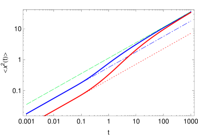
Figure 1: (Color online) Graphical representation of the MSD (9) on log-log scale. The blue solid line (upper solid line) corresponds to the MSD in the case of two backbones, $l_{1}=0$, $l_{2}=L=1$, and $w_{1}=w_{2}=1/2$. The blue dot-dashed line describes the asymptotic behavior of the MSD for short times, given by (11). The red solid line (lower solid line) corresponds to the MSD in case of five backbones, $l_{j}=(j-1)L$, $j=1,2,\dots,5$, $L=1$, $w_{j}=1/5$. The red dotted line corresponds to its asymptotic behavior for short times, given by (11). The MSDs in both cases have the same asymptotic in the long time limit given by (10), i.e. $\left\langle x^{2}(t)\right\rangle=\frac{2\mathcal{D}_{x}}{\sqrt{\mathcal{D}_{y}}}\frac{t^{1/2}}{\Gamma\left(1/2\right)}$ (green dashed line). Diffusion coefficients are set to 1; $\mathcal{D}_{x}=\mathcal{D}_{y}=1$.

From relations (10) and (11) we conclude that any finite number of backbones does not change the transport exponent in the short and long time limit. In the intermediate times there is more complicated behavior of the MSD given by relation (9). The crossover time scales separating the behavior at short, intermediate, and long times are given by $t_{short}=\min\{l_{j}^{2},j>1\}/2\mathcal{D}_{y}=l_{2}^{2}/2\mathcal{D}_{y}$ and $t_{long}=\max\{l_{j}^{2}\}/2\mathcal{D}_{y}=l_{N}^{2}/2\mathcal{D}_{y}$.

In the presence of a constant external force $F$ along the backbones we arrive at the following Fokker-Planck equation

$$\frac{\partial}{\partial t}P(x,y,t)= \sum_{j=1}^{N}w_{j}\delta(y-l_{j})\left[-\eta F\frac{\partial}{\partial x}+\mathcal{D}_{x}\frac{\partial^{2}}{\partial x^{2}}\right]$$ (14)

$$\times P(x,y,t)+\mathcal{D}_{y}\frac{\partial^{2}}{\partial y^{2}}P(x,y,t),$$

where $\eta$ is the mobility. One can compute the first moment as a function of time,

$$\left\langle x(t)\right\rangle_{F}=\frac{\eta F}{2\sqrt{\mathcal{D}_{y}}}\mathcal{L}^{-1}\left[s^{-3/2}\sum_{j=1}^{N}w_{j}e^{-\sqrt{\frac{s}{\mathcal{D}_{y}}}|l_{j}|}\right],$$

where by comparing it with relation (8) we conclude that the generalized Einstein relation is fulfilled metzler report ,

$$\left\langle x(t)\right\rangle_{F}=\frac{F}{2k_{B}T}\left\langle x^{2}(t)\right\rangle_{F=0},$$ (16)

where $\eta k_{B}T=\mathcal{D}_{x}$.

III Fractal structure of backbones

To introduce a fractal structure of the backbones we go back to Eq.(2) and replace the summation $\sum_{j=1}^{N}w_{j}\delta(y-l_{j})$ with summation over a fractal set $\mathcal{S}_{\nu}$, i.e., $\sum_{l_{j}\in\mathcal{S}_{\nu}}\delta(y-l_{j})$, which means that the backbones are at positions $y$ which belong to the fractal set $\mathcal{S}_{\nu}$ with fractal dimension $0<\nu<1$.

A simple toy example, which corresponds to an infinite fractal set, can be treated as follows. In relation (8) we calculate $\sum_{j=1}^{N}w_{j}e^{-\sqrt{\frac{s}{\mathcal{D}_{y}}}|l_{j}|}\rightarrow\sum_{l_{j}\in\mathcal{S}_{\nu}}e^{-\sqrt{\frac{s}{\mathcal{D}_{y}}}|l_{j}|}$. One should recognize that fractal sets (like a Cantor set) are uncountable. Therefore, the last expression is purely formal and its mathematical realization corresponds to integration to fractal measure $\mu_{\nu}\sim l^{\nu}$ such that $\sum_{l_{j}\in\mathcal{S}_{\nu}}\delta(l-l_{j})=\frac{1}{\Gamma(\nu)}l^{\nu-1}$ is the fractal density SKM book ; tarasov , and $d\mu_{\nu}=\frac{1}{\Gamma(\nu)}l^{\nu-1}dl$. Here we note that $\mathcal{D}_{x}$ is a generalized diffusion coefficient with physical dimension $[\mathcal{D}_{x}]=\mathrm{m}^{3-\nu}/\mathrm{s}$ that absorbs the dimension of fractal volume or measure $\mu_{\nu}$. That finally yields the following integration:

$$\frac{1}{\Gamma(\nu)}\int_{0}^{\infty}dl\,l^{\nu-1}e^{-\sqrt{\frac{s}{\mathcal{D}_{y}}}l}=\left(\frac{\mathcal{D}_{y}}{s}\right)^{\nu/2}.$$ (17)

For the MSD, we obtain from (8)

$$\left\langle x^{2}(t)\right\rangle=\frac{\mathcal{D}_{x}}{\mathcal{D}_{y}^{\frac{1-\nu}{2}}}\frac{t^{\frac{1+\nu}{2}}}{\Gamma\left(1+\frac{1+\nu}{2}\right)},$$ (18)

i.e., anomalous diffusive behavior with the transport exponent equal to $\frac{1}{2}<\frac{1+\nu}{2}<1$. Thus, the fractal set $\mathcal{S}_{\nu}$ of the infinite number of backbones changes the transport exponent, from $1/2$ to $\frac{1+\nu}{2}$. For $\nu=1$ the MSD becomes $\left\langle x^{2}(t)\right\rangle\simeq t$, which is consistent with expectations, and for $\nu=0$, we are back to the finite-$N$ case. Indeed, the fractal dimension of any finite number of discrete points is $\nu=0$.

We further consider a random fractal set $\mathcal{S}_{\nu}\in[a,b]$, with finite limits. From relation (8), in the same way as in (17), for a finite integration in $[0,L]$, one finds a result in the form of an incomplete $\gamma$ function $\gamma(a,x)=\int_{0}^{x}dt\,t^{a-1}e^{-t}$ erdelyi ,

$$\frac{1}{\Gamma(\nu)}\int_{0}^{L}dl\,l^{\nu-1}e^{-\sqrt{\frac{s}{\mathcal{D}_{y}}}l}=\left(\frac{\mathcal{D}_{y}}{s}\right)^{\nu/2}\frac{\gamma(\nu,L)}{\Gamma(\nu)}.$$ (19)

Thus, the MSD becomes

$$\left\langle x^{2}(t)\right\rangle=\frac{\mathcal{D}_{x}}{\mathcal{D}_{y}^{\frac{1-\nu}{2}}}\frac{\gamma(\nu,L)}{\Gamma(\nu)}\frac{t^{\frac{1+\nu}{2}}}{\Gamma\left(1+\frac{1+\nu}{2}\right)}.$$ (20)

Again, for $\nu=1$ the normal diffusive behavior along the $x$ direction appears, i.e., $\left\langle x^{2}(t)\right\rangle\simeq t$.

Here we note that the result for the MSD (18) can be obtained in the framework of fractional integration as well. By integration of Eq.(2) over $y$ and using the summation on the fractal set as above in this section, for the PDF $p_{1}(x,t)$ one obtains

$$\frac{\partial}{\partial t}p_{1}(x,t)=\mathcal{D}_{x}\sum_{l_{j}\in\mathcal{S}_{\nu}}\frac{\partial^{2}}{\partial x^{2}}p(x,y=l_{j},t).$$ (21)

The Laplace transform to (21) yields

$$s\hat{p}_{1}(x,s)-p_{1}(x,t=0)=\mathcal{D}_{x}\sum_{l_{j}\in\mathcal{S}_{\nu}}\frac{\partial^{2}}{\partial x^{2}}\hat{p}(x,y=l_{j},s).$$ (22)

By representing the solution $p(x,y,s)$ in the following way: $\hat{p}(x,y,s)=\hat{g}(x,s)e^{-\sqrt{\frac{s}{\mathcal{D}_{y}}}|y|}$, i.e., $\hat{p}(x,y=l_{j},s)=\hat{g}(x,s)e^{-\sqrt{\frac{s}{\mathcal{D}_{y}}}|l_{j}|}$, for the $\hat{p}_{1}(x,s)$ we find

$$\hat{p}_{1}(x,s)=\int_{-\infty}^{\infty}dyp(x,y,s)=2\hat{g}(x,s)\sqrt{\frac{\mathcal{D}_{y}}{s}}.$$ (23)

From the other side, by using the previous approach of summation, we have

$$\sum_{l_{j}\in\mathcal{S}_{\nu}}\hat{p}(x,y=l_{j},s) =\hat{g}(x,s)\frac{1}{\Gamma(\nu)}\int_{0}^{\infty}dll^{\nu-1}e^{\sqrt{\frac{s}{\mathcal{D}_{y}}}l}$$ (24)

$$=\hat{g}(x,s)\left(\frac{\mathcal{D}_{y}}{s}\right)^{\nu/2}$$

$$=\frac{1}{2\mathcal{D}_{y}^{\frac{1-\nu}{2}}}s^{\frac{1-\nu}{2}}\hat{p}_{1}(x,s).$$

By substituting relation (24) in (22), we obtain

$$s^{\frac{1+\nu}{2}}\hat{p}_{1}(x,s)-s^{\frac{1+\nu}{2}-1}p_{1}(x,t=0)$$

$$=\frac{\mathcal{D}_{x}}{2\mathcal{D}_{y}^{\frac{1-\nu}{2}}}\frac{\partial^{2}}{\partial x^{2}}\hat{p}_{1}(x,s).$$ (25)

From this, the inverse Laplace transform yields the following time fractional diffusion equation:

$$\frac{\partial^{\frac{1+\nu}{2}}}{\partial t^{\frac{1+\nu}{2}}}p_{1}(x,t)=\frac{\mathcal{D}_{x}}{2\mathcal{D}_{y}^{\frac{1-\nu}{2}}}\frac{\partial^{2}}{\partial x^{2}}p_{1}(x,t),$$ (26)

where $\frac{\partial^{\frac{1+\nu}{2}}}{\partial t^{\frac{1+\nu}{2}}}$ is the Caputo time fractional derivative of order $\frac{1}{2}<\frac{1+\nu}{2}<1$ Caputo ; caputo derivative . From here we easily obtain the MSD $\left\langle x^{2}(t)\right\rangle=\int_{-\infty}^{\infty}dxx^{2}p_{1}(x,t)$ that is of form (18). The solution for the PDF $p_{1}(x,t)$ can be represented in terms of the Fox $H$ function $H_{p,q}^{m,n}(z)$ saxena book ; sandev jpa2011 ,

$$p_{1}(x,t)=\frac{1}{2|x|}H_{1,1}^{1,0}\left[\left.\frac{|x|}{\sqrt{\mathcal{D}_{\nu}t^{(1+\nu)/2}}}\right|\begin{array}[]{c l}(1,(1+\nu)/4)\\ (1,1)\end{array}\right],$$ (27)

where $\mathcal{D}_{\nu}=\mathcal{D}_{x}/2\mathcal{D}_{y}^{\frac{1-\nu}{2}}$ is the generalized diffusion coefficient with physical dimension $[\mathcal{D}_{\nu}]=\mathrm{m}^{2}/\mathrm{s}^{(1+\nu)/2}$. Therefore, as shown, the infinite number of backbones changes the transport exponent.

The asymptotic behavior of $p_{1}(x,t)$ (27) for $\frac{|x|}{\sqrt{\mathcal{D}_{\nu}t^{(1+\nu)/2}}}\gg 1$ is of the form metzler report ; sandev jpa2011 :

$$p_{1}(x,t)\simeq \frac{1}{\sqrt{2(3-\nu)\pi}}\left(\frac{1+\nu}{4}\right)^{\frac{\nu-1}{3-\nu}}|x|^{\frac{\nu-1}{3-\nu}}\left(\mathcal{D}_{\nu}t^{\frac{1+\nu}{2}}\right)^{-\frac{1}{3-\nu}}$$ (28)

$$\times\exp\left[-\frac{3-\nu}{4}\left(\frac{1+\nu}{4}\right)^{\frac{1+\nu}{3-\nu}}|x|^{\frac{4}{3-\nu}}\left(\mathcal{D}_{\nu}t^{\frac{1+\nu}{2}}\right)^{-\frac{2}{3-\nu}}\right],$$

i.e., it has non-Gaussian behavior. For $\nu=1$ it turns to Gaussian behavior as it is expected and as it was shown by analysis of the MSD.

Additionally to the MSD we calculate the $q$th moment $\left\langle|x|^{q}\right\rangle=2\int_{0}^{\infty}dx\,x^{q}p_{1}(x,t)$, for which one finds metzler report ; sandev jpa2011

$$\left\langle|x|^{q}\right\rangle=\left(\mathcal{D}_{\nu}t^{\frac{1+\nu}{2}}\right)^{q/2}\frac{\Gamma(1+q)}{\Gamma\left(1+\frac{1+\nu}{2}\frac{q}{2}\right)}.$$ (29)

Thus for the fourth moment it follows that

$$\left\langle|x|^{4}\right\rangle=24\mathcal{D}_{\nu}^{2}\frac{t^{1+\nu}}{\Gamma(2+\nu)}=6\frac{\mathcal{D}_{x}^{2}}{\mathcal{D}_{y}^{1-\nu}}\frac{t^{1+\nu}}{\Gamma(2+\nu)}.$$ (30)

The calculation of the fourth moment is useful to discriminate subdiffusive processes with identical MSDs, e.g., subdiffusion due to different fractal structures or different mechanisms spanner (see also metzler pccp ). For the even moments we obtain

$$\left\langle|x|^{2n}\right\rangle=(2n)!\frac{\mathcal{D}_{\nu}^{n}t^{\frac{(1+\nu)n}{2}}}{\Gamma\left(1+\frac{(1+\nu)n}{2}\right)},$$ (31)

from which we can find the following interesting relation:

$$\sum_{n=0}^{\infty}\frac{\left\langle|x|^{2n}\right\rangle}{(2n)!}=\sum_{n=0}^{\infty}\frac{\mathcal{D}_{\nu}^{n}t^{\frac{(1+\nu)n}{2}}}{\Gamma\left(1+\frac{(1+\nu)n}{2}\right)}=E_{(1+\nu)/2}\left(\mathcal{D}_{\nu}t^{\frac{1+\nu}{2}}\right),$$

where $E_{\alpha}(z)=\sum_{n=0}^{\infty}\frac{z^{n}}{\Gamma(\alpha n+1)}$ is the one parameter Mittag-Leffler function saxena book .

IV Weierstrass function and fractional Riesz derivative

Finally, we show how the fractal structure $\mathcal{S}_{\nu}$ relates to the fractional Riesz derivative SKM book . Let us consider the fractal structure of backbones in Eq.(2) separately. In the Fourier-Fourier $\left(\kappa_{x},\kappa_{y}\right)$ space it reads

$$-\mathcal{D}_{x}\kappa_{x}^{2}\sum_{j=1}^{\infty}w_{j}e^{i\kappa_{y}l_{j}}\bar{\tilde{P}}(\kappa_{x},y=l_{j},t)$$

$$=-\mathcal{D}_{x}\kappa_{x}^{2}\sum_{j=1}^{\infty}w_{j}e^{i\kappa_{y}l_{j}}\frac{1}{2\pi}\int_{-\infty}^{\infty}d\kappa_{y}{{}^{\prime}}\bar{\tilde{P}}(\kappa_{x},\kappa_{y}{{}^{\prime}},t)e^{-i\kappa_{y}{{}^{\prime}}l_{j}}$$

$$=-\mathcal{D}_{x}\kappa_{x}^{2}\frac{1}{2\pi}\int_{-\infty}^{\infty}d\kappa_{y}{{}^{\prime}}\Psi\left(\kappa_{y}-\kappa_{y}{{}^{\prime}}\right)\bar{\tilde{P}}(\kappa_{x},\kappa_{y}{{}^{\prime}},t),$$ (33)

where $\Psi\left(\kappa_{y}-\kappa_{y}{{}^{\prime}}\right)$ is the Weierstrass function berry . It can be obtained by the following procedure shlesinger : Let us use $w_{j}=\frac{l-b}{b}\left(\frac{b}{l}\right)^{j}$, where $l,b>1$, $l-b\ll b$. Thus

$$\sum_{j=1}^{\infty}w_{j}=\frac{l-b}{l}\sum_{j=0}^{\infty}\left(\frac{b}{l}\right)^{j}=1.$$ (34)

Now $l$ and $b$ are dimensionless scale parameters. Therefore

$$\Psi(z)=\frac{l-b}{b}\sum_{j=1}^{\infty}\left(\frac{b}{l}\right)^{j}\exp\left(i\frac{z}{l^{j}}\right),$$ (35)

where $l_{j}=L/l^{j}$, and $z=\left(\kappa_{y}-\kappa_{y}{{}^{\prime}}\right)L$, and for convenience, we choose $l_{1}=L$. From here one obtains

$$\Psi(z/l)=\frac{l}{b}\Psi(z)-\frac{l-b}{b}\exp\left(i\frac{z}{l}\right).$$ (36)

Neglecting the last term since $l-b\ll b$, therefore the scaling

$$\Psi(z/l)\simeq\frac{l}{b}\Psi(z),$$ (37)

means that $\Psi(z)\sim\frac{1}{z^{1+\nu}}$, where $\nu=\ln\frac{1}{b}/\ln{l}$ is the fractal dimension. Thus, for relation (IV) we have

$$-\mathcal{D}_{x}\kappa_{x}^{2}\frac{L^{-1-\nu}}{2\pi}\int_{-\infty}^{\infty}d\kappa_{y}{{}^{\prime}}|\kappa_{y}-\kappa_{y}{{}^{\prime}}|^{-1-\nu}\bar{\tilde{P}}(\kappa_{x},\kappa_{y}{{}^{\prime}},t).$$

This integration is the Riesz fractional derivative SKM book .

V Summary

In this paper we introduce a diffusion equation for a comb structure where the displacements in the $x$ direction are possible along many backbones, even an infinite number of backbones, and we call this system by grid comb. We analyze the MSD and we show that by adding a finite number of backbones, the transport exponent in the long time limit does not change. Differently from that, an infinite number of backbones changes the transport exponent. Considering a fractal structure of backbones with fractal dimension $\nu$ we obtained the dependence of the transport exponent on $\nu$. We stress that the performed analysis is exact–more precisely, that the evaluation of the contribution of the fractal structure $\mathcal{S}_{\nu}$ to anomalous diffusion is exact. Note that the first attempt to take into account a fractal structure of traps was performed in iomin2 in the framework of a coarse graining procedure of the Fokker-Planck equation that leads to the fractional differentiation in the real space. In contrast to that, in the present analysis we are able to perform an exact analysis for the fractal structure $\mathcal{S}_{\nu}$. This also relates to exact fractional differentiation in the reciprocal Fourier space.

In conclusion, it should be admitted that a comb model is a toy model that can be solved exactly and establishes a relation between geometry and the transport exponent. As is recently found it also corresponds to the real physical realization in experiments on calcium transport in spiny dendrites (see mendez ; iomin and references therein). The grid-comb model, suggested here as the generalization of the comb model, establishes an exact relation between a complicated fractal geometry and the transport exponent as well. Another strong motivation of the model, also related to the result, is that in the framework of this model it is possible to infer an exactly fractional derivative related to fractal geometry. All these points are important for the understanding of anomalous transport in heterogeneous material, in particular to describe diffusion of solvents in thin porous films Shamiryan , or in another two-dimensional material like graphene ruzicka .

References

• (1) S.R. White and M. Barma, J. Phys. A: Math. Gen. 17, 2995 (1984).
• (2) G.H. Weiss and S. Havlin, Physica A 134, 474 (1986).
• (3) O. Matan, S. Havlin, and D. Staufler, J. Phys. A: Math. Gen. 22, 2867 (1989).
• (4) V.E. Arkhincheev and E.M. Baskin, Sov. Phys. JETP 73, 161 (1991).
• (5) R. Metzler and J. Klafter, Phys. Rep. 339, 1 (2000); J. Phys. A: Math. Gen. 37, R161 (2004).
• (6) V.E. Arkhincheev, Chaos, 17, 043102 (2007).
• (7) E. Baskin and A. Iomin, Phys. Rev. Lett. 93, 120603 (2004).
• (8) L.R. da Silva, A.A. Tateishi, M.K. Lenzi, E.K. Lenzi, and P.C. da Silva, Braz. J. Phys. 39, 483 (2009).
• (9) D. Cassi and S. Regina, Phys. Rev. Lett. 76, 2914 (1996); G. Baldi, R. Burioni, and D. Cassi, Phys. Rev. E 70, 031111 (2004).
• (10) V. Mendez and A. Iomin, Chaos Solitons Fractals 53, 46 (2013).
• (11) A. Iomin and V. Mendez, Phys. Rev. E 88, 012706 (2013).
• (12) A. Iomin, Phys. Rev. E 83, 052106 (2011).
• (13) A. Iomin, Phys. Rev. E 86, 032101 (2012).
• (14) Y. Sagi, M. Brook, I. Almog, and N. Davidson, Phys. Rev. Lett. 108, 093002 (2012).
• (15) E.K. Lenzi, L.R. da Silva, A.A. Tateishi, M.K. Lenzi, and H.V. Ribeiro, Phys. Rev. E 87, 012121 (2013).
• (16) K. Maex, M.R. Baklanov, D. Shamiryan, F. Lacopi, S.H. Brongersma, and Z.S. Yanovitskaya, J. Appl. Phys. 93, 8793 (2003).
• (17) I.M. Sokolov, in Encyclopedia of Complexity and Systems Science, edited by R.A. Mayers (Springer-Verlag, New York, 2009), p. 309.
• (18) J.-F. Gouyet, Physics and Fractal Structures (Masson, Paris, 1996).
• (19) N. Korabel and E. Barkai, Phys. Rev. Lett. 104, 170603 (2010).
• (20) V.E. Arkhincheev, E. Kunnen, and M.R. Baklanov, Microelectron. Eng. 88, 694 (2011).
• (21) A. Iomin and E. Baskin, Phys. Rev. E 71, 061101 (2005).
• (22) D. Shamiryan, M.R. Baklanov, P. Lyons, S. Beckx, W. Boullart, and K. Maex, Colloids Surf., A 300, 111 (2007).
• (23) A. Rebenshtok and E. Barkai, Phys. Rev. E 88, 052126 (2013).
• (24) A. Erdelyi, W. Magnus, F. Oberhettinger and F.G. Tricomi, Higher Transcedential Functions, (McGraw-Hill, New York, 1955), Vol. 3.
• (25) S.G. Samko, A.A. Kilbas, and O.I. Marichev, Fractional Integrals and Derivatives: Theory and Applications (Taylor and Francis, London, 1993).
• (26) V.E. Tarasov, Chaos 14, 123 (2004).
• (27) M. Caputo, Elasticita e Dissipazione (Zanichelli, Bologna) 1969.
• (28) The Caputo fractional derivative of order $0<\mu<1$ is defined by $\frac{\partial^{\mu}}{\partial t^{\mu}}f(t)=\frac{1}{\Gamma(1-\mu)}\int_{0}^{t}\mathrm{d}\tau(t-\tau)^{-\mu}\frac{d}{d\tau}f(\tau)$ Caputo . Its Laplace transform is given by $\mathcal{L}\left[\frac{\partial^{\mu}}{\partial t^{\mu}}f(t)\right](s)=s^{\mu}\mathcal{L}\left[f(t)\right](s)-s^{\mu-1}f(0+)$.
• (29) A.M. Mathai, R.K. Saxena and H.J. Haubold, The $H$-function: Theory and Applications (Springer, New York, 2010).
• (30) T. Sandev, R. Metzler, and Z. Tomovski, J. Phys. A: Math. Theor. 44, 255203 (2011).
• (31) M. Spanner, F. Höfling, G. Schröder-Turk, K. Mecke, and T. Franosch, J. Phys.: Condens. Matter 23, 234120 (2011).
• (32) R. Metzler, J.-H. Jeon, A.G. Cherstvy, and E. Barkai, Phys. Chem. Chem. Phys. 16, 24128 (2014).
• (33) M.V. Berry and Z.V. Lewis, Proc. R. Soc. London Ser. A 370, 459 (1980).
• (34) M.F. Shlesinger, J. Stat. Phys. 10, 421 (1974).
• (35) B.A. Ruzicka, S. Wang, L.K. Werake, B. Weintrub, K.P. Loh, and H. Zhao, Phys. Rev. B 82, 195414 (2010).