The high-order Euler method and the spin-orbit model
A fast algorithm for solving differential equations with small, smooth nonlinearity

Abstract

We present an algorithm for the rapid numerical integration of smooth, time-periodic differential equations with small nonlinearity, particularly suited to problems with small dissipation. The emphasis is on speed without compromising accuracy and we envisage applications in problems where integration over long time scales is required; for instance, orbit probability estimation via Monte Carlo simulation. We demonstrate the effectiveness of our algorithm by applying it to the spin-orbit problem, for which we have derived analytical results for comparison with those that we obtain numerically. Among other tests, we carry out a careful comparison of our numerical results with the analytically predicted set of periodic orbits that exists for given parameters. Further tests concern the long-term behaviour of solutions moving towards the quasi-periodic attractor, and capture probabilities for the periodic attractors computed from the formula of Goldreich and Peale. We implement the algorithm in standard double precision arithmetic and show that this is adequate to obtain an excellent measure of agreement between analytical predictions and the proposed fast algorithm.

1 Motivation

In this paper, we discuss an algorithm for the rapid numerical solution of smooth, nonlinear, non-autonomous, time-periodic, dissipative differential equations, with reference to a particular example, known as the spin-orbit equation. The spin-orbit ordinary differential equation (ODE) describes the coupling, in the presence of tidal friction, between the orbital and rotational motion of an ellipsoidal satellite orbiting a primary, and many authors have studied it since the original work of [Danby (1962)] and [Goldreich and Peale (1966)]; see also [Murray and Dermott (1999)], [Celletti (2010)] and [Correia and Laskar (2004)]. In cases of interest, both the nonlinear and the dissipative terms are multiplied by small parameters, and as the dissipation parameter decreases, the ODE possesses an ever-increasing number of co-existing periodic orbits, with the initial conditions selecting which one is observed. In this sense, the problem is not simple, despite the fact that the nonlinearity is small: small dissipation coupled with small nonlinearity leads here to non-trivial dynamics.

One interesting application of the spin-orbit equation is as a model of the orbit of Mercury, whose primary is considered to be the Sun; other applications come to mind with the discovery of extra-solar planetary systems. The orbit of Mercury appears to be unique in the solar system, since it rotates three times on its own axis for every two orbits of the Sun: all other regular satellites for which we have data are in a one-to-one resonance with their primaries. See for instance [Noyelles et al. (2013)] for a recent survey offering a new perspective on the problem.

In order to estimate numerically the probability of capture of a satellite in a given orbit, one possibility is to use a Monte Carlo approach, in which the spin-orbit ODE is integrated forward in time, starting from many uniformly-distributed random initial conditions. The time-asymptotic behaviour, that is, the solution after any transient has decayed, is determined for each of these initial conditions, and the probability of capture by each of the possible attractors is thereby estimated. The challenges of this approach are (a) that realistic values of the dissipation parameter $\gamma$ are small, so transient times, which are $O(1/\gamma)$ — see [Bartuccelli et al. (2012)] for an argument in a similar case — are long; and (b), in order to obtain low-error estimates of capture probabilities, a large number $I$ of initial conditions must be considered: in fact, the width of the 95% confidence interval for the probabilities is proportional to $I^{-1/2}$ — see equation (10). In interesting cases, that is when $\gamma$ is small, (a) and (b) force one to carry out a large number of simulations of orbit dynamics, each one over a long time interval, which, using traditional numerical ODE solvers, requires prohibitively long computation times. For a problem such as this, we therefore conclude that a fast ODE solving algorithm is a necessity and not a luxury.

Many problems in mathematical physics boil down to solving an ODE for which no closed-form solution exists. For simulations in such cases, there is no alternative but to approximate solutions numerically. Also, the solutions to nonlinear problems can display sensitive dependence to initial conditions. This raises questions as to how good a representation of what we casually refer to as ‘the solution’ to an initial value problem, is actually obtainable numerically. Contrast a finite precision numerical solution to the notional ‘true solution’ — one which is computed to infinitely high precision, but the computation of which can be done in a finite time. Clearly the latter is unattainable with real computing hardware, with its finite memory and speed. Hence, in practice, the best we can do is to use finite-precision, usually double precision (typically 16–17 significant figures) algorithms, to model, approximately, the true solution.

Although software for arbitrary-precision arithmetic is available, we want to show here what can be achieved using only double precision (with one exception). The question then becomes: how might we construct a practical algorithm to approximate the true solution, using standard double precision arithmetic, while also bearing in mind the need to obtain solutions quickly?

We describe in this paper an algorithm that speeds up the solution process by a factor of at least 7 compared to ‘traditional’ numerical ODE solvers, such as standard algorithms like Runge-Kutta [Press et al. (1992), Asher and Petzold (1998)] and symplectic numerical methods, for instance the Yoshida algorithm [Yoshida (1990), Celletti (2010), Appendix F]. The latter has been used to solve the spin-orbit problem in the past, for example in [Celletti and Chierchia (2008)]. These algorithms and many more like them are general-purpose methods that work for a wide variety of problems. By contrast, our algorithm is specific to a particular problem, but, since it is set up by computer algebra, only small changes need to be made to the set-up code in order to modify it for a different problem; with this proviso, our algorithm is also general-purpose.

Our algorithm works well for problems like the spin-orbit ODE, for which we carry out a careful comparison of our numerical results with those obtained analytically, via perturbation theory, as well as published results on attractor probabilities, in order to validate our work. Setting up the algorithm relies on computer algebra, and running the algorithm at speed requires a low-level computer language; the interplay between these two forms of computation is a theme in the paper.

The rest of the paper is organised as follows. The spin-orbit ODE is given and a fast solution algorithm is described in Sect. 2. Details on setting up the algorithm and some practical data are given in Sect. 3, and verification is reported in Sect. 4. In Sect. 5, we give details of the speed and the robustness of the algorithm, and in Sect. 6 we draw some conclusions. The perturbation theory calculations which underpin the verifications are carried out in the Appendix, which also contains some further supplementary material.

2 The ODE and a fast solution algorithm

We consider the spin-orbit ODE:

$$\begin{cases}\dot{x}=y,\\ \dot{y}=-\varepsilon\,G(x,t)-\gamma\alpha\left(y-\omega\right).\end{cases}$$ (1)

where $\alpha,\varepsilon,\gamma,\omega>0$ and $x\in\mathds{T}=\mathds{R}/\pi\mathds{Z}$, so that the phase space is $\mathds{T}\times\mathds{R}$. Here $\varepsilon$ is a small parameter, related to the asymmetry of the equatorial moments of inertia of the satellite, and $e$ is the eccentricity of the orbit [Goldreich and Peale (1966), Murray and Dermott (1999)]. From here onwards we set $\dot{x}=y$. We follow [Goldreich and Peale (1966), Celletti and Chierchia (2008), Celletti and Chierchia (2009)] in setting $\omega=\nu(e)=\overline{N}(e)/\overline{L}(e)$; we also write $\overline{L}(e)=\alpha$, where

$$\overline{L}(e)=\frac{1+3e^{2}+3e^{4}/8}{(1-e^{2})^{9/2}}\;\;\;\mbox{ and }\;\;\;\overline{N}(e)=\frac{1+15e^{2}/2+45e^{4}/8+5e^{6}/16}{(1-e^{2})^{6}}.$$

Furthermore,

$$G(x,t)=\sum_{k\in\mathcal{K}}A_{k}(e)\sin(2x-kt),\;\;\;\mbox{ where }\;\;\;\mathcal{K}=\{-3,-2,-1,1,2,3,4,5,6,7\}$$ (2)

and

$$A_{-3}={\frac{81}{1280}}\,{e}^{5} A_{-2}=\frac{1}{24}\,{e}^{4}$$

$$A_{-1}={\frac{1}{48}}\,{e}^{3}+{\frac{11}{768}}\,{e}^{5} A_{1}=-\frac{1}{2}\,e+\frac{1}{16}\,{e}^{3}-{\frac{5}{384}}\,{e}^{5}$$

$$A_{2}=1-\frac{5}{2}\,{e}^{2}+{\frac{13}{16}}\,{e}^{4} A_{3}=\frac{7}{2}\,e-\frac{123}{16}\,e^{3}+{\frac{489}{128}}\,e^{5}$$

$$A_{4}={\frac{17}{2}}\,{e}^{2}-{\frac{115}{6}}\,{e}^{4} A_{5}={\frac{845}{48}}\,{e}^{3}-{\frac{32525}{768}}\,{e}^{5}$$

$$A_{6}={\frac{533}{16}}\,{e}^{4} A_{7}={\frac{228347}{3840}}\,{e}^{5}.$$

The expressions for $\overline{L}(e)$ and $\overline{N}(e)$ have been obtained by averaging, and those for $A_{k}(e)$ have been derived by solving the Kepler relations up to $O(e^{6})$ [Celletti and Chierchia (2008)], truncation at this order leading to the neglect of all harmonics outside the set $\mathcal{K}$.

The dissipation model in equation (1) is known as MacDonald’s tidal torque [MacDonald (1964), Murray and Dermott (1999)]. It has been widely studied since the pioneering work of Goldreich and Peale [Goldreich and Peale (1966)], even though its validity has recently been questioned; see for instance [Noyelles et al. (2013)] and references therein, and also the comments at the end of Sect. 6. It should be noted that the probability of capture will be affected by the choice of dissipation model.

The algorithm to solve (1) that we propose in this paper is essentially the usual Euler method, extended so that the series solution is computed to $O(h^{N})$, where $h$ is the timestep and $N\gg 1$. That is, we advance a solution by one timestep via the truncated Taylor expansion

$$\mathbf{x}(t_{i})=\mathbf{H}(\mathbf{x}(t_{i-1}),t_{i-1})=\mathbf{x}(t_{i-1})+\sum_{j=1}^{N}\frac{h^{j}}{j!}\,\mathbf{f}_{j}(\mathbf{x}(t_{i-1}),t_{i-1}),$$ (3)

where $t_{i}=t_{0}+ih$, ${\bf x}(t)=(x(t),y(t))$ and the functions ${\bf f}_{j}$ can be computed explicitly from the differential equation, which allows one to compute, recursively, the derivatives of $x(t)$ and $y(t)$ of all orders at $t=t_{i-1}$, in terms of the initial conditions, $x(t_{i-1})$, $y(t_{i-1})$. The standard Euler method can be recovered by setting $N=1$.

With a judicious choice of $N$ and $h$, we demonstrate that for our problem, one can use (3) to compute solutions to the ODE in relatively large, equal timesteps. Furthermore, the size of the timestep used is fixed throughout, so the algorithm is not even adaptive. Such an approach might be thought to be of limited practical use, but it is one purpose of this paper to show that, for some problems, this is not the case. In particular, the computational cost of solving an ODE using the proposed method turns out to be lower than all other algorithms against which it was compared.

We draw a parallel here between this work and that of, for instance, [Saari (1970), Chang and Corliss (1980)], in which a series approach is also used to solve ODEs. There are however important differences between the approach of Chang and Corliss and ours: first, the series used by them are computed, numerically, at each timestep; and second, they use appropriate variations on the standard ratio test for convergence, to estimate the size of each timestep — so their method is adaptive. By contrast, in this work, the timesteps are fixed and all series required are pre-computed and stored: this approach can significantly speed up the algorithm by reducing the computational overheads. Both methods are, however, essentially numerical analytical continuation.

In setting up our algorithm, we use computer algebra (CA) to generate code in a low-level language (LL), once only for each set of parameters, which computes the functions appearing on the right-hand side of equation (3). This LL code is in turn compiled and executed in order to produce results. It might be thought that the LL step can be omitted, and the CA program can be used to carry out the whole task. It can; this approach would lead to a significant decrease in speed however, since CA software is generally designed for algebraic manipulation and is not optimised for numerical computation. As an example, consider the sum

$$S(n)=\sum_{i=1}^{n}\frac{(i+1)(i+3)}{i(i+2)(i+4)(i+6)},\;\;\;\mbox{ where }\;\;\;\lim_{n\rightarrow\infty}S(n)=\frac{9}{32},$$ (4)

whose evaluation requires $6n-1$ addition and $5n$ multiplication/division operations, and which we use later for timing purposes. The obvious experiment shows that numerical evaluation of $S(n)$, for $n$, say, $10^{6}$, using 17 significant figures, takes about 260 times longer using CA compared with LL. This increase in speed comes at a cost however: standard LL codes using in-built mathematical operations, although relatively fast, will always carry out arithmetic to fixed precision — double precision is standard, which equates to about 16–17 s.f. On the other hand, CA can in principle be used to evaluate numerical expressions to any specified precision, the upper limit being set only by memory and time constraints. This implied trade-off between accuracy and speed guides us in setting up the algorithm in practice. The compromise we have to make is encapsulated in:

Find the smallest integer $N$ and the largest fixed timestep $h$, such that the pair of power series of degree $N$, which advance the solution $\mathbf{x}(t)$ of (1) from $t=ih$ to $t=(i+1)h$, using (3), for all $i\in\mathds{N}$, both do so to within a given tolerance.

Increasing $h$ increases speed, since larger timesteps are used, and increasing $N$ and/or decreasing $h$ both increase accuracy in principle, but the exact relationship between these parameters is not straightforward, since rounding errors come into play. It is clear, though, that since the differential equation (1) is $2\pi$-periodic in $t$, we need to find the smallest integer $M$, where $h=2\pi/M$, such that a suitable error criterion is met for the finite set $i=1,\ldots,M$, for all initial conditions $\mathbf{x}(0)$ in some subset $\mathcal{Q}$ of $\mathds{R}^{2}$, in order for it to be met for all $i\in\mathds{N}$.

In order to quantify numerical error, we compare estimates of the state vector $\mathbf{x}(t)=(x(t),y(t))$ at a time $t=T_{1}$, computed from the state vector at $t=T_{0}$, where $T_{1}>T_{0}$, with the computation being carried out in two ways: using a high-precision numerical ODE solver (which we denote with the subscript ‘num’), and our high-order Euler method (which we label ‘hem’).

Hence, the requirements of the computer algebra software are:

1. efficient series manipulation;

2. ability to translate arbitrary algebraic expressions into a low-level language;

3. ability to carry out floating point arithmetic to any given precision;

4. a selection of algorithms for purely numerical solution of differential equations.

Items (3) and (4) above are necessary for making error estimates. The numerical algorithm chosen was a Gear single-step extrapolation method using Bulirsch-Stoer rational extrapolation [Press et al. (1992)], which is good for computing high-accuracy solutions to smooth problems. We make the assumption that results produced by this algorithm, for $h\in[0,2\pi]$, $t_{0}\in[0,2\pi]$ and initial conditions in $\mathcal{Q}$, are both accurate (that is, close to the true solution) and precise (that is, correct to a large number of significant figures). In fact, using 30 significant figures for computation, and relative and absolute error parameters of $10^{-20}$, we believe that numerical solutions accurate to about 20 s.f. can be obtained, and it is against these that our algorithm is compared.

The computer algebra software Maple has all the necessary attributes and was used for this work; the low-level language used was C.

The approach we adopt is partly experimental, in that we show that the power series we obtain meet the error criterion described in Sect. 3, by comparing high-accuracy numerical solutions from CA with those produced by our algorithm, implemented in LL, and then using the results to choose optimal values of $N$, the series truncation order, and $M$, the number of timesteps per period of $2\pi$.

In more detail, the computation of $\mathbf{f}_{i}$ in (3) is carried out as follows. The method of Frobenius assumes that the solution to an ODE, expanded about the point $t=t_{0}$, can be written as an infinite series, so that $x(t)=\sum_{i=0}^{\infty}a_{i}(t-t_{0})^{i}$. Substituting this into (1) gives a recursion formula for $a_{i+1}$ in terms of $a_{j},\,j=0\ldots i$. Hence, given $a_{0}$ and $a_{1}$, which correspond to the two initial conditions $x_{0}=x(t_{0})$ and $y_{0}=\dot{x}(t_{0})$, we can find $a_{j}$ for $j=2\ldots N$, where $N$ can in principle be as large as desired.

Since the ODE (1) is nonlinear, so is the recursion formula, and the closed-form expressions for $a_{i}(e,\varepsilon,\gamma,x_{0},y_{0},t_{0})$, as polynomials in the six arguments, quickly become large as $i$ increases. Hence, practical considerations, principally memory and computer time constraints, (a) force us to minimise the number of unevaluated parameters — we use the minimum, just two, $x_{0}$ and $y_{0}$, substituting numerical values for the others — and (b) bound the value of $N$. For the specific case of the spin-orbit problem, it has been found to be feasible to use $N$ up to at least 20. This part of the computation is carried out by CA.

Our ultimate goal is to estimate the relative areas of the basins of attraction of each of the attractive periodic solutions to equation (1), for given values of the parameters $\varepsilon$ and $\gamma$. A Monte Carlo approach is one possible way to do this. For the case at hand, this approach requires us first to compute $\mathbf{x}_{j}=(x_{j},y_{j})=\left(x(2j\pi),y(2j\pi)\right)$, $j=1\ldots J$ for a sufficiently large $J$ that any transient behaviour has effectively decayed away, and for a large number $I$ of uniformly-distributed random initial conditions $\mathbf{x}_{0}=(x_{0},y_{0})$ in a given set $\mathcal{Q}$. From now on, we drop the subscript 0 on the initial conditions where this does not lead to confusion. Clearly we need an efficient means for computing the Poincaré map $\mathbf{P}:\mathbb{R}^{2}\mapsto\mathbb{R}^{2}$ generated by (1), which is defined by $\mathbf{x}_{k+1}=\mathbf{P}(\mathbf{x}_{k})$. In practice, $\mathbf{P}$ cannot be computed from the series solution in $M=1$ step: this would require $h=2\pi/M=2\pi$ in the series for $x(t)$ and $y(t)$, and this is certainly too large. Moveable singularities of the solution in complex-time would prevent the series from converging for such a timestep. Hence, we split $\mathbf{P}$ into $M$ ‘sub-maps’ so that $\mathbf{P}(\mathbf{x})=\mathbf{p}_{M}\circ\mathbf{p}_{M-1}\circ\ldots\circ\mathbf{p}_{1}(\mathbf{x})$, where $\mathbf{p}_{i}(\mathbf{x})=(X_{i}(\mathbf{x}),Y_{i}(\mathbf{x}))$, with $X_{i}$ advancing $x$ from $t=(i-1)h$ to $t=ih$ and $Y_{i}$ advancing $y$ over the same interval. In terms of the function $\mathbf{H}$ in equation (3), we set $t_{0}=0$ and $\mathbf{x}=\mathbf{x}(t_{i-1})$, from which $\mathbf{p}_{i}(\mathbf{x})=\mathbf{H}(\mathbf{x},t_{i-1})$.

With $h=2\pi/M$, we have

$$X_{i}(\mathbf{x})=\sum_{j=0}^{N}a_{i,j}(\mathbf{x})\,h^{j}+O\left(h^{N+1}\right)\;\;\;\mbox{ and }\;\;\;Y_{i}(\mathbf{x})=\sum_{j=0}^{N-1}(j+1)a_{i,j+1}(\mathbf{x})\,h^{j}+O\left(h^{N}\right),$$ (5)

where $i=1,\ldots,M$. Also, $\mathbf{x}=(x(t_{i-1}),y(t_{i-1}))$ is the solution and its derivative at $t_{i-1}=(i-1)h$; and $a_{i,j}(\mathbf{x})$ are polynomials in $y,\,\cos 2x,\,\sin 2x$ if $j>0$, with an additional linear term in $x$ if $j=0$. We designate this algorithm the high-order Euler method (HEM).

In practice, the expressions for $X_{i}(\mathbf{x})$ and $Y_{i}(\mathbf{x})$, $i=1,\ldots,M$, are computed for particular numerical values of $e$, $\varepsilon,\gamma,N$ and $h$. The fact that the spin-orbit equation (1) is also $\pi$-periodic in $x$ implies that the functions $X$ and $Y$, for fixed $M$ and $N$ and with numerical values for $e$, $\varepsilon,\gamma$ and $h$, can be written in one of two forms. The first of these is the Fourier form

$$X_{i}(\mathbf{x}) = x+A_{i,0}(y)+\sum_{j=1}^{F}\varepsilon^{j}\left[A_{i,j}(y)\cos 2jx+B_{i,j}(y)\sin 2jx\right],$$

$$Y_{i}(\mathbf{x}) = C_{i,0}(y)+\sum_{j=1}^{F}\varepsilon^{j}\left[C_{i,j}(y)\cos 2jx+D_{i,j}(y)\sin 2jx\right],$$ (6)

where $F$ is a positive integer and $A_{i,j},\ldots D_{i,j}$ are polynomials in $y$, $h$ and the parameters of the problem. Both $F$ and the degree of the polynomials depend on our accuracy requirements and on $N$; typically, we find $F\approx 3$ for $\varepsilon\leq 10^{-3}$. The fact that $A_{i,j}(y),\ldots D_{i,j}(y)$ always have a common factor of $\varepsilon^{j}$ is explained in Appendix D. The second (polynomial) form is equivalent to the Fourier form and is

$$X_{i}(\mathbf{x})=x+\sum_{i,j,k}\alpha_{i,j,k}\varepsilon^{j+k}y^{i}c^{j}s^{k},\;\;\;\;Y_{i}(\mathbf{x})=\sum_{i,j,k}\beta_{i,j,k}\varepsilon^{j+k}y^{i}c^{j}s^{k},$$ (7)

where $\alpha_{i,j,k},\,\beta_{i,j,k}$ are constants, and from here onwards, we set $c=\cos 2x$, $s=\sin 2x$. In practice, we use CA to compute $X_{i}$ and $Y_{i},\,i=1,\ldots,M$ in the polynomial form, to convert these into Horner form [Press et al. (1992)] for efficient evaluation, and then to translate the result into LL. There turns out to be very little difference in the computational effort required to evaluate these expressions in the Fourier and polynomial forms, and in this work we choose the latter.

3 Setting up the algorithm

We now study a pair of cases in more detail. Throughout this section, we let $\mathcal{Q}=[0,\pi]\times[0,y_{\mathrm{max}}]$ be the set of initial conditions, with $y_{\mathrm{max}}=5$. The first component of the initial condition need only be in the range $0$ – $\pi$ because the spin-orbit equation is $\pi$-periodic in $x$. We also follow [Celletti and Chierchia (2008)] in fixing $e=0.2056$, the value appropriate to Mercury, so that $\omega\approx 1.25584$; $\varepsilon=10^{-3}$; and $\gamma=10^{-5}$ and $10^{-6}$, giving $\gamma\alpha\approx 1.36937\times 10^{-5}$ and $1.36937\times 10^{-6}$ respectively. All numerical computations in CA are carried out to 30 s.f. We refer to these parameter values, with $\gamma$ excluded, as the default parameters. The default value of $e$ and the other parameter values are chosen because we can then compare our results using HEM directly with results published in [Celletti and Chierchia (2008)], which were obtained using a Yoshida symplectic integrator [Yoshida (1990)], [Celletti (2010), Appendix F].

$N$	$M$	Total no. of	Total $+/\times$ ops.	(Max $e_{x}$, Max $e_{y}$), $\times 10^{-14}$	(Max $e_{x}$, Max $e_{y}$), $\times 10^{-14}$
		terms in $\mathbf{P}(\mathbf{x})$	(Horner form)	$\gamma=10^{-5}$	$\gamma=10^{-6}$
18	18	6698	4597/4650	2582.6, 464.1	2586.9, 464.2
	19	6914	4821/4866	734.2, 55.6	734.2, 55.7
	20	7109	4994/5112	267.0, 21.1	267.0, 21.1
	22	7433	5314/5400	46.0, 3.7	46.0, 3.6
	25	7994	5872/5949	5.9, 0.54	5.4, 0.56
	28	8396	6359/6455	4.1, 0.45	4.4, 0.52
	31	8780	6780/6807	3.8, 0.54	4.2, 0.45
19	22	7992	5685/5779	11.7, 0.98	10.0, 0.86
	25	8526	6270/6350	3.8, 0.47	4.1, 0.46
	28	8906	6750/6870	3.5, 0.51	4.4, 0.60
20	19	7967	5492/5608	44.6, 2.5	43.0, 2.8
	20	8153	5715/5824	16.3, 1.0	14.0, 1.1
	21	8346	5888/6067	6.9, 0.56	6.6, 0.63
	22	8512	6042/6170	4.6, 0.45	3.8, 0.50
	25	9042	6666/6741	4.3, 0.47	5.0, 0.50

Table 1: How the number of arithmetical operations required to compute one iteration of the Poincaré map, and the approximate maximum error obtained when using the high-order Euler Method, vary with $N$ and $M$. The maximum error is an estimate of $\max_{\mathbf{x}_{0}\in\mathcal{Q}}(e_{x}(\mathbf{x}_{0}),e_{y}(\mathbf{x}_{0}))$.

We first use CA to set up the functions $\mathbf{p}_{i}(\mathbf{x})$ and then translate them into LL. A priori, we have no idea what values of $M$ and $N$ to choose, and a compromise between high accuracy, which tends to increase $M$ and $N$, and speed of the HEM, which increases with decreasing $M$, must be found. Additionally, finite computer memory puts a bound on $N$, since the expressions for $a_{i,j}(\mathbf{x})$ in equation (5) grow rapidly in size with $j$. Furthermore, the fact that these expressions will eventually be evaluated using finite-precision arithmetic means that increasing $N$ and $M$ too much can result in a less accurate approximation to the Poincaré map, owing to the fact that more operations are required to evaluate the expressions, potentially leading to increased rounding errors.

We define our measure of error as follows. Letting $\mathbf{x}_{0}=\mathbf{x}(t_{0})$, we define the error vector $\mathbf{e}(\mathbf{x}_{0})=(e_{x},e_{y})$ by

$$e_{x}=\left|x_{\mathrm{num}}(\mathbf{x}_{0},t_{0}+2\pi)-x_{\mathrm{hem}}(\mathbf{x}_{0},t_{0}+2\pi)\right|,\;\;e_{y}=\left|y_{\mathrm{num}}(\mathbf{x}_{0},t_{0}+2\pi)-y_{\mathrm{hem}}(\mathbf{x}_{0},t_{0}+2\pi)\right|.$$ (8)

In practice, we estimate the maximum values of $e_{x}(\mathbf{x}_{0})$ and $e_{y}(\mathbf{x}_{0})$, with $t_{0}=0$, as $\mathbf{x}_{0}$ ranges over a grid of uniformly-spaced points in $\mathcal{Q}$. The points used are $\{\mathbf{x}_{0}=(i\,\Delta x,j\,\Delta y),\,i,j=0\ldots L\}$ with $\Delta x=\pi/L$ and $\Delta y=y_{\mathrm{max}}/L$, and $L=25$.

We now establish good values of $M$ and $N$. Table 1 gives data to guide the choice of values that represents a compromise between accuracy and speed. The total number of terms and operation count data, which are almost the same for both $\gamma=10^{-5}$ and $10^{-6}$, are given to enable us to judge the relative speed, and the $e_{x},e_{y}$ values indicate the accuracy.

The main point to note is that for fixed $N$, the maximum error varies little with $M$ for $M\geq M_{\mathrm{crit}}$, but for $M<M_{\mathrm{crit}}$, the error increases rapidly: there is a ‘knee’ in the error curve at $M=M_{\mathrm{crit}}$. From several possible candidates, we choose $N=18$ and $M=28$, which represents a good speed/accuracy compromise both for $\gamma=10^{-5}$ and $10^{-6}$.

Description	$\gamma=10^{-5}$	$\gamma=10^{-6}$
1. Total CPU time for computing $X_{i}(\mathbf{x})$, $Y_{i}(\mathbf{x})$,
$i=1,\ldots M$, using CA. Without error check.	255 CPU-sec	262 CPU-sec
2. As 1., but with error check.	3143 CPU-sec	2550 CPU-sec
3. Total no. of terms in $\mathbf{P}(\mathbf{x})$, before/after pruning	20578/8396
4. Number of $+/\times$ operations (pruned, not Horner)	6349/55550
5. Number of $+/\times$ operations (pruned, Horner form)	6359/6455
6. $\mbox{[Maximum value of $(e_{x},e_{y})$]}\times 10^{-14}$	$(4.1,0.45)$	$(4.4,0.52)$

Table 2: Data on the computer algebra set-up of the low-level language code to compute the Poincaré map.

Table 2 gives some data on setting up $\mathbf{P}(\mathbf{x})$ with $N=18$ and $M=28$. Points to note, with numbers in the list corresponding to line numbers in the table, are:

1. The timings are given here in units of seconds of CPU time on a particular computer. For comparison, the LL-evaluation of $S(6\times 10^{7})$ defined in equation (4), using the same computer, takes about 1 CPU-sec.

2. The error check is an estimate of the maximum values of $e_{x}(\mathbf{x}_{0})$ and $e_{y}(\mathbf{x}_{0})$, defined in equation (8), with $t_{0}=0$, as $\mathbf{x}_{0}$ ranges over a grid of uniformly-spaced points in $\mathcal{Q}$, as defined immediately following equation (8). We set $L=25$, so that $\Delta x=\pi/25$ and $\Delta y=0.2$.

3. The total number of terms in the expressions for $X_{i}(\mathbf{x})$, $Y_{i}(\mathbf{x})$, $i=1,\ldots,M$ in the polynomial form — equation (7) — is given in row 3 in the table. A ‘term’ is a single product of the form $\alpha_{i,j,k}y^{i}c^{j}s^{k}$ appearing in equation (7).

   ‘Pruning’ is a way of cutting down the number of terms retained by removing the negligible ones. Specifically, any terms for which $|\alpha_{i,j,k}\,y_{\mathrm{max}}^{i}|<T_{\mathrm{max}}$ are deleted, with $T_{\mathrm{max}}=10^{-18}$. This value of $T_{\mathrm{max}}$ was chosen because the final expressions will be computed in in LL using double precision arithmetic (equivalent to about 17 s.f.). Pruning with $T_{\mathrm{max}}=10^{-18}$ reduces the number of terms in $\mathbf{P}(\mathbf{x})$ by about a half.

4. This row gives a measure of the computational cost — the total number of addition and multiplication operations — of evaluating $\mathbf{P}(\mathbf{x})$ in the polynomial form. Evaluating a term $y^{k}$ is assumed to take $k-1$ multiplications.

5. The total number of multiplication operations is reduced by a factor of about eight when the expressions are converted to Horner form.

6. For the given parameters, the maximum difference between one iteration of the Poincaré map computed using (a) HEM and (b) a high-precision numerical ODE solver, is of order $10^{-14}$. The values given are an approximation to $\max_{\mathbf{x}_{0}\in\mathcal{Q}}\left(e_{x}(\mathbf{x}_{0}),e_{y}(\mathbf{x}_{0})\right)$, as defined in equation (8) with $t_{0}=0$.

4 Verification

We now verify the HEM in three ways. In the first of these, we check that the set of periodic and quasi-periodic solutions obtained numerically via the HEM corresponds with those that can be proved to exist analytically, for example by perturbation theory. In the second verification, the probability of obtaining the different attractors is estimated, again using the HEM, and these probabilities are compared with the results published in [Celletti and Chierchia (2008)] — here, we are of course comparing one numerical algorithm (HEM), against another (a Yoshida symplectic integrator). We also compare attractor probabilities given by the formula of Goldreich and Peale [Goldreich and Peale (1966)] with those obtained from HEM. In the third verification, we compute $\omega^{\prime}$ (defined in the Appendix and discussed below) numerically, using the HEM, and compare this value with that given by perturbation theory.

All the verifications relate to the default parameters, which are listed at the start of Sect. 3. The probability computations using HEM are carried out in the standard way: $I$ uniformly-distributed random initial conditions in $\mathcal{Q}$ are selected and the Poincaré map is iterated $n_{\mathrm{pre}}$ times, starting from each one. Since the transient time is $O(1/\gamma)$ [Bartuccelli et al. (2012)], we use $n_{\mathrm{pre}}=10^{6}$ for $\gamma=10^{-5}$ and $n_{\mathrm{pre}}=5\times 10^{7}$ for $\gamma=10^{-6}$. For the other values of $\gamma$ used later in the paper, we also choose $n_{\mathrm{pre}}=m/\gamma$, with $m\approx 10$ being chosen such that, after integrating for a time $2\pi n_{\mathrm{pre}}$, any transients have decayed to the point where the solution can be identified.

4.1 Which attractors exist?

As shown in the Appendix, for $\gamma=10^{-5}$, the quasi-periodic solution and periodic solutions with $p/q=1/2,\,1/1,\,5/4,\,3/2,\,2/1,\,5/2$ and $3/1$ exist according to a second order analysis, and no others. For $\gamma=10^{-6}$, these solutions remain, and additional solutions with $p/q=3/4,\,7/4$ and $7/2$ also exist. All of these, and only these solutions are observed when using the HEM, although only two out of the $I=32000$ random initial conditions were attracted to the $p/q=3/4$ solution. Since the threshold for this solution is $\gamma=1.058\times 10^{-6}$, we would expect the probability of observing it to be very small. A posteriori we expect that higher order periodic solutions do not arise for the chosen values of the parameters — or, at worst, are irrelevant.

4.2 The quasi-periodic solution

A quasi-periodic solution to (1) can also exist, as discussed in the Appendix. This solution has a mean growth rate, $\omega^{\prime}$, which, for small $\varepsilon$, is close to $\omega$. Equation (24) implies a formula for estimating $\omega^{\prime}$, which is

$$\omega^{\prime}=\lim_{t\rightarrow\infty}\left[\frac{x(t)-x(0)}{t}\right]=\lim_{n\rightarrow\infty}\left[\frac{x(2\pi n)-x(0)}{2\pi n}\right].$$ (9)

The second version is appropriate here, since we use the HEM to compute iterations of the Poincaré map, and so only have access to values of $(x(t),\dot{x}(t))$ at $t=2n\pi$, $n=0,1,2,\ldots$.

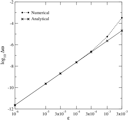
Figure 1: Comparison of analytical and numerical computations of $\Delta\omega=\omega-\omega^{\prime}$ for various values of $\varepsilon$. For small $\varepsilon$, the values of $\Delta\omega$ are seen to agree, thereby validating the HEM, which was used to produce the numerical results.

Starting from equation (42) in the Appendix, we have that

$$\omega^{\prime}=\omega-\varepsilon^{2}\mu^{(2)}(\omega^{\prime})+O(\varepsilon^{3})=\omega-\varepsilon^{2}\mu^{(2)}(\omega)+O(\varepsilon^{3}),$$

where we have used the fact that, since $\omega^{\prime}$ and $\omega$ differ by $O(\varepsilon^{2})$, replacing $\mu^{(2)}(\omega^{\prime})$ with $\mu^{(2)}(\omega)$ makes a difference $O(\varepsilon^{4})$, which can be neglected. From equation (39) we compute $\mu^{(2)}(\omega)=2.284502$. In Fig. 1 we plot the analytical estimate of $\Delta\omega=\omega-\omega^{\prime}=\varepsilon^{2}\mu^{(2)}(\omega)$ and the numerical estimate from (9), using LL, for $n=10^{8}$, $\gamma=10^{-5}$ and $\varepsilon\in\{10^{-5},3\times 10^{-5},10^{-4},3\times 10^{-4},10^{-3},3\times 10^{-3}\}$. Additionally, we estimate $\Delta\omega$ for $\varepsilon=10^{-6}$, but in this case, double precision arithmetic is inadequate — this the single case, referred to in Sect. 1, where we do not use double precision. Details of this computation are given in Sect. C of the Appendix.

This is very different kind of test of the HEM compared to that described in the previous section. Here, we check that the long-term average rate of increase of $x$ implied by equation (9) is as predicted by the analytical computation.

4.3 Estimated attractor probabilities

We estimate the probability $P(p/q)$ that integrating forward in time from a randomly-selected initial condition $\mathbf{x}\in\mathcal{Q}$ leads to a period-$p/q$ orbit. If several periodic orbits with a given $p$, $q$ exist, then their combined probability is computed.

	Probability, $P(p/q)$, %
$p/q$	$\gamma=10^{-5}$		$\gamma=10^{-6}$
	From CC	This work	From CC	This work
1/2	NO	$0.50\pm 0.08$	NO	$0.62\pm 0.09$
3/4	NE	NE	NO	$0.0063(\pm 0.009)$
1/1	$4.7\pm 1.3$	$4.58\pm 0.23$	$4.6\pm 1.3$	$4.77\pm 0.23$
5/4	$8.4\pm 1.7$	$7.31\pm 0.29$	$5.1\pm 1.4$	$7.50\pm 0.29$
$\omega^{\prime}$	$69.8\pm 2.9$	$71.65\pm 0.49$	$73.4\pm 2.7$	$70.22\pm 0.50$
3/2	$12.6\pm 2.1$	$12.05\pm 0.36$	$14.0\pm 2.2$	$11.94\pm 0.36$
7/4	NE	NE	NO	$0.094\pm 0.03$
2/1	$2.9\pm 1.0$	$2.72\pm 0.18$	$2.5\pm 0.97$	$3.01\pm 0.19$
5/2	$1.1\pm 0.7$	$0.97\pm 0.11$	$0.2(\pm 0.28)$	$1.13\pm 0.12$
3/1	$0.5\pm 0.4$	$0.22\pm 0.05$	$0.2(\pm 0.28)$	$0.48\pm 0.08$
7/2	NE	NE	NO	$0.24\pm 0.05$

Table 3: Attractor probabilities with their 95% confidence intervals, determined using $I=1000$ points, taken from CC [Celletti and Chierchia (2008)]; and 32000 points (this work). NO: attractor exists but was not observed; NE: attractor non-existent for these parameters. The 95% confidence interval in parentheses is not reliable since for this case, $\widehat{p}I<5$. The Poincaré map was iterated a total of about $1.6\times 10^{12}$ times to produce the probability data for $\gamma=10^{-6}$.

We also compute the 95% confidence interval for these probabilities, using the formula for the standard error of a proportion [Walpole et al. (1998)]. This states that if a number $I$ of initial conditions is considered; $\widehat{p}$ is the number of those initial conditions that end up on a given attractor $A$, divided by $I$; and $Z_{c/2}$ is defined by

$$\frac{1}{\sqrt{2\pi}}\int_{-Z_{c/2}}^{Z_{c/2}}e^{-z^{2}/2}\,dz=c,\;\;\;\mbox{ where $c\in[0,1]$};$$

then a $c\times 100\%$ confidence interval for the actual proportion $p$ of initial conditions going to $A$ is

$$p\in\left[\widehat{p}-Z_{c/2}\sqrt{\frac{\widehat{p}(1-\widehat{p})}{I}},\;\widehat{p}+Z_{c/2}\sqrt{\frac{\widehat{p}(1-\widehat{p})}{I}}\right].$$ (10)

This estimate is reliable provided that $I\widehat{p}\geq 5$ [Walpole et al. (1998)]. Setting $c=0.95$ corresponds to a 95% confidence interval and gives $Z_{0.475}\approx 1.96$. Clearly, the width of the confidence interval is proportional to $I^{-\frac{1}{2}}$, as stated in Sect. 1.

Note that the simulations reported in [Celletti and Chierchia (2008)] do not find all possible periodic orbits. Take the case $p/q=1/2$ for $\gamma=10^{-5}$. From Table 3, we have $P(1/2)\in[4.2\times 10^{-3},\,5.8\times 10^{-3}]$ with 95% confidence. From the binomial distribution, one can compute that the probability of this orbit not being observed at all in 1000 simulations is less than $0.015$.

The periodic orbit probabilities for $\gamma=10^{-5}$ and $10^{-6}$ are given in Table 3. Note that the results for $\gamma=10^{-6}$ in [Celletti and Chierchia (2008)] were obtained by polynomial extrapolation from larger $\gamma$ values and the 95% confidence intervals, added by us, were computed assuming that $I=1000$. Extrapolation in a case like this can be risky, because when taking smaller values of $\gamma$ the orbit probabilities do not increase indefinitely, but tend to settle around a constant value; this has been observed numerically in [Bartuccelli et al. (2012)] for a system with cubic nonlinearity, but we believe this to be a general phenomenon. In our case, $\varepsilon=10^{-3}$ with $e=0.2056$, the value of $\gamma$ where this appears to happen is around $\gamma=10^{-5}$, and the constant value of $P(3/2)$ for $\gamma<10^{-5}$ is about 12%.

There is a further check that we can carry out, based on the formula of Goldreich and Peale [Goldreich and Peale (1966)]. Using an averaging technique, this formula approximates the probability of capture in a particular $p:q$ resonance, with $q=2$, as follows:

$$P_{GP}(p)=\frac{2}{1+\frac{\pi(p/2-\omega)}{2\sqrt{2\varepsilon A_{p}(e)}}},$$

where $A_{p}(e)$ is defined straight after equation (2). The formula can be seen to be $\gamma$-independent, but, for small enough $\gamma$, gives probability estimates in good agreement with those given by HEM, as shown in Table 4.

		Probability, $P(3/2)$, %
$\epsilon$	$\gamma$		$y\in[1.5,2]$		$y\in[1.5,5]$
		G & P	HEM, all terms	HEM, $A_{3}$ only	HEM, all terms	HEM, $A_{3}$ only
	$10^{-8}$	7.70	$9.17\pm 0.48$	$9.56\pm 0.44$	$7.82\pm 0.41$	$8.34\pm 0.42$
	$10^{-7}$	7.70	$9.84\pm 0.48$	$9.16\pm 0.33$	$7.43\pm 0.47$	$7.84\pm 0.38$
$1.8\times 10^{-4}$	$10^{-6}$	7.70	$9.28\pm 0.37$	$9.49\pm 0.45$	$7.92\pm 0.34$	$7.88\pm 0.42$
	$10^{-5}$	7.70	$9.02\pm 0.36$	$8.77\pm 0.36$	$7.48\pm 0.37$	$7.48\pm 0.33$
	$10^{-4}$	7.70	$5.73\pm 0.29$	$5.61\pm 0.29$	$4.61\pm 0.27$	$4.62\pm 0.27$
	$10^{-7}$	17.24	$20.3\pm 0.47$		$16.0\pm 0.43$
	$10^{-6}$	17.24	$20.6\pm 0.42$		$16.6\pm 0.27$
$1.0\times 10^{-3}$	$10^{-5}$	17.24	$20.2\pm 0.28$		$16.3\pm 0.47$
	$10^{-4}$	17.24	$19.0\pm 0.34$		$15.8\pm 0.46$
	$10^{-3}$	17.24	$8.59\pm 0.36$		$6.80\pm 0.32$

Table 4: Comparison of the probability of capture by the 3:2 orbit, for $x\in[0,\pi],y\in[1.5,2]$ and $y\in[1.5,5]$, as computed by G&P, the formula of Goldreich and Peale [Goldreich and Peale (1966)] and also by the high-order Euler method, HEM. The $\pm$ quantities after the HEM probabilities are the width of the 95% confidence interval. These are given to two significant figures so that, $I$, the number of initial conditions used, can be deduced if required, by using equation (10).

The Goldreich and Peale formula is obtained under a series of approximations, one of which consists in assuming that the solution is close to a given resonance. That is, the formula computes the probability of capture for a solution passing near the given resonance and the possibility that the solution is captured by other resonances is neglected. Since, on physical grounds, we are interested in trajectories in which the speed of rotation decreases with time, it might be expected that the best choice would be to take the initial data above the resonance 3:2 and below the next higher resonance, i.e. $y\in[1.5,2]$. However, as Table 4 shows, the Goldreich and Peale formula better describes the behaviour of trajectories starting in the full phase space above the resonance. The presence of the other resonances apparently does not affect the probability of capture by the 3:2 resonance. We also considered a modified model of the form (1), where only the harmonic with $k=3$ is kept in $G(x,t)$. Here we found that the probability of capture in the 3:2 resonance is essentially the same as for the full spin-orbit model; apparently the basins of attraction of the other resonances are formed at the expense of the basin of attraction of the quasi-periodic attractor, leaving that of the 3:2 resonance unaffected.

5 Performance of the high-order Euler method

5.1 Speed

The HEM was developed as a fast numerical solver for the spin-orbit ODE and problems like it. Hence, we now compare the timings for solving (1) using HEM, with those from two other numerical methods. We choose an explicit Runge-Kutta method due to Dormand and Price, as described in [Hairer et al. (1993)], and an adaptive Taylor series method due to Jorba and Zou (TSM) [Jorba and Zou (2005)].

Parameters	Tolerance	HEM time,	Ratio (DOP853)	Ratio (Taylor
		CPU-sec		series method)
$\rule[-1.72218pt]{0.0pt}{12.91663pt}\varepsilon=1.2\times 10^{-4}$, $\gamma=10^{-7}$	$3.6\times 10^{-15}$	17.22	21.1	11.7
$\rule[-1.72218pt]{0.0pt}{12.91663pt}\varepsilon=1.8\times 10^{-4}$, $\gamma=10^{-8}$	$4.4\times 10^{-15}$	18.86	19.0	11.0
$\rule[-1.72218pt]{0.0pt}{12.91663pt}\varepsilon=10^{-3}$, $\gamma=5\times 10^{-6}$	$4.5\times 10^{-14}$	19.04	14.2	7.97
$\rule[-1.72218pt]{0.0pt}{12.91663pt}\varepsilon=10^{-3}$, $\gamma=10^{-6}$	$2.1\times 10^{-14}$	20.93	16.3	9.05
$\rule[-1.72218pt]{0.0pt}{12.91663pt}\varepsilon=3\times 10^{-3}$, $\gamma=10^{-5}$	$4.2\times 10^{-14}$	24.44	12.6	6.92

Table 5: Comparison of timings for the high-order Euler method (HEM) versus a Runge-Kutta code (DOP853) and a Taylor series method. The timings are the mean from three computations, in each of which the Poincaré map was iterated 50 000 times starting from each of 50 random initial conditions — hence $2.5\times 10^{6}$ iterations for each computation. For HEM, the actual time in CPU-sec is given; the last two columns give the ratio of the time taken by the named algorithm to the time taken by HEM.

The results are summarised in Table 5, in which we compare the data on the time taken for each of the algorithms to perform $2.5\times 10^{6}$ iterations of the Poincaré map. Specifically, if we define the test problem as ‘iterate the Poincaré map 50 000 times starting from each of 50 random initial conditions in $\mathcal{Q}$’, then the time used to produce Table 5 is the mean of the time taken to run the test problem three times, using a different set of initial conditions on each occasion. Note that the figure in the ‘HEM time’ column is a number of CPU-sec, where 1 CPU-sec is the time taken to compute $S(6\times 10^{7})$, defined in equation (4). By contrast, the figures in the two ‘Ratio’ columns are the ratios of the times taken by the named algorithms to the time taken by HEM.

We have been at pains to make the comparisons as fair as possible, which is why the tolerance is different for each of the five sets of parameters: the values chosen correspond closely to the estimated tolerance in the HEM method for those parameters. We take this precaution because the time taken by both Runge-Kutta and TSM depends sensitively on the value of tolerance used.

It can be seen from Table 5 that HEM outpaces both the algorithms against which it has been tested by a factor of at least 6.9:1, with the factor depending on the parameters. It is noteworthy that the time taken by HEM is not strongly correlated with the value of $\gamma$, with, in particular, the smaller (and physically more interesting) values of dissipation not significantly slowing down the computation: in fact, there is evidence that smaller values of $\gamma$ lead to a relative increase in speed of HEM compared to the other algorithms.

It may be thought surprising that HEM is noticeably faster than TSM, since both are based on analytical continuation. A quick experiment for the first set of parameters in Table 5 shows that, typically, the TSM takes about 15.5 timesteps to advance a solution of the spin-orbit ODE by a time $2\pi$, which is comparable with $M$, the number used in HEM ($M\approx 20-30$). Hence, the likely reason for the difference in speed is that, since TSM is an adaptive algorithm, the Taylor series for the solution must be re-computed at every timestep. This results in a larger computational overhead compared to HEM, where the series are computed once only, saved, and then merely evaluated as required in order to compute the Poincaré map.

5.2 Robustness

We now give some results that illustrate the robustness of the computation of attractor probabilities using HEM. We deliberately choose sub-optimal values of $M$ that result in higher maximum values of $(e_{x},e_{y})$, the absolute error per iteration of the Poincaré map. The data are given in Table 6, from which it can be concluded that the probabilities computed with all three values of $M$ agree at the 95% confidence level in the cases considered.

	Probability, $P(p/q)$, %
$p/q$	$M=28$	$M=20$	$M=19$	$M=18$
	$\mathbf{E}=(4.1,0.45)$	$\mathbf{E}=(267,21)$	$\mathbf{E}=(734,56)$	$\mathbf{E}=(2583,464)$
1/2	$0.50\pm 0.08$	$0.48\pm 0.08$	$0.42\pm 0.07$	$0.47\pm 0.08$
1/1	$4.58\pm 0.23$	$4.60\pm 0.23$	$4.76\pm 0.23$	$4.79\pm 0.23$
5/4	$7.31\pm 0.29$	$7.53\pm 0.29$	$7.39\pm 0.29$	$7.61\pm 0.29$
$\omega^{\prime}$	$71.65\pm 0.49$	$71.06\pm 0.50$	$71.02\pm 0.50$	$70.73\pm 0.50$
3/2	$12.05\pm 0.36$	$12.35\pm 0.36$	$12.18\pm 0.36$	$12.07\pm 0.36$
2/1	$2.72\pm 0.18$	$2.72\pm 0.18$	$2.87\pm 0.18$	$3.05\pm 0.19$
5/2	$0.97\pm 0.11$	$0.99\pm 0.11$	$1.08\pm 0.11$	$1.03\pm 0.11$
3/1	$0.22\pm 0.05$	$0.27\pm 0.06$	$0.28\pm 0.06$	$0.24\pm 0.05$

Table 6: Demonstration of the robustness of the computation of attractor probabilities when $\gamma=10^{-5}$, $N=18$ and the other parameters take the default values. For comparison, the $M=28$ column repeats the results in Table 3. The error estimates are $\mathbf{E}=\max_{\mathbf{x}_{0}\in\mathcal{Q}}(e_{x},e_{y})\times 10^{-14}$, and are taken from Table 1. For all solutions and all values of $M$, the 95% confidence intervals overlap.

6 Discussion and Conclusions

Weierstrass’ Approximation Theorem [Handscomb (1966)] (real, multivariate polynomial version) states:

If $f$ is a continuous real-valued function defined on the set $[a,b]\times[c,d]$ and $\delta>0$, then there exists a polynomial function $p$ in two variables such that $|f(x,y)-p(x,y)|<\delta$ for all $x\in[a,b]$ and $y\in[c,d]$.

In the light of this, it is not surprising that, for large enough degree $N$, and number of timesteps per $2\pi$, $M$, the Frobenius method can give very good approximations to the functions $X_{i}(\mathbf{x})$, $Y_{i}(\mathbf{x})$, $i=1,\ldots,M$, that go to build up the Poincaré map, $\mathbf{P}(\mathbf{x})$, and hence, to $\mathbf{P}(\mathbf{x})$ itself. Less obvious is how effective a numerical ODE solver based on such series approximations — the high-order Euler method (HEM) as we call it — can be in practice.

In this paper, we have applied the HEM to a particular problem, the spin-orbit problem, to illustrate its effectiveness in solving this nonlinear ODE. We maintain that this is a non-trivial problem, in the sense that the set of solutions can consist of many coexisting periodic orbits as well as one quasi-periodic solution. We show here that not only is the HEM capable of finding all the solutions predicted by perturbation theory, and finds none that are not so predicted, but it also enables us to compute accurately the mean frequency of the quasi-periodic solution and to make estimates of the probabilities of the various coexisting attractors which agree with published results and the Goldreich-Peale formula (where it applies). Additionally, compared to standard numerical techniques, not only does HEM find all anticipated solutions, but it is also about 40 times faster. All this is achieved by using standard double precision arithmetic.

This increased speed comes at the cost of setting up the functions $X_{i}(\mathbf{x})$, $Y_{i}(\mathbf{x})$, which map the solution and its derivative forward by a time $h$, where $h=2\pi/M$ is a timestep which is relatively large since in practice $M\sim 25$. Before the advent of computer algebra this approach would have been impracticable for anything more than very small $N$ — in fact, too small, given our accuracy requirements — but such software is readily available nowadays and the process of setting up these functions is easily automated.

It would be useful to be able to define the class of ODEs for which HEM is a good numerical algorithm. It not straightforward to define such a class, although it is clear that all functions appearing in the ODE must be sufficiently many times differentiable, in order for the Frobenius method to work. When the dissipation is large, any standard ODE solver would work; however, HEM comes into its own for problems with small dissipation. Additionally, if the nonlinearity is multiplied by a small parameter, conjecturally that may help to improve convergence — see equations (6) and (7).

Further work is needed to investigate whether, for the spin-orbit problem at least, the range of $y$-values can be extended. In fact, we have carried out computations which show that the HEM works for at least $y\in[-5,10]$, although at the cost of increasing $M$ to 35–40. For $y$-values outside this range, we envisage that the polynomials $A_{i,j}(y)\ldots D_{i,j}(y)$ in equation (7) might be better replaced by a rational form, by using, for example, a Padé approximation [Press et al. (1992)].

Of interest too is the possibility that the technique described in [Saari (1970)], which uses a conformal transformation of the independent variable to extend the radius of convergence of a power series solution to an ODE, might be applied to the spin-orbit problem, thereby allowing us to decrease $M$ and so further speed up our algorithm. Another question for investigation is whether there exists a form in which the Poincaré map can be represented that can be computed in significantly fewer arithmetical operations than we have used here.

Recently, it has been argued that MacDonald’s model does not provide a realistic description of the tidal torque and leads to inconsistencies [Makarov (2012), Williams and Efroimsky (2012), Noyelles et al. (2013)]. In this paper, we have used MacDonald’s torque model in equation (1) both for purposes of comparison with existing literature — in particular, [Celletti and Chierchia (2008), Goldreich and Peale (1966)] — and because its simplicity makes it particularly suitable for analytical calculations. It would be interesting to investigate to what extent our method could be applied to more general situations, such as those envisaged in the papers quoted above.

Acknowledgements

The Authors wish to acknowledge the helpful comments received from the anonymous reviewers, which have strengthened the paper by bringing to our attention the freely available software (DOP853 and the adaptive Taylor series method) with which our algorithm has been compared in Section 5.1.

Appendix: perturbation theory computations

Appendix A Perturbation theory: periodic attractors

We carry out here the perturbation theory computations necessary to establish thresholds for the periodic and quasi-periodic solutions which we observe numerically. Details concerning this type of computation can be found in [Coddington and Levinson (1955), Verhulst (1990), Gentile (2006), Gentile (2009)].

A.1 First order computation

We consider (1) with $\gamma=\varepsilon\,C_{1}+\varepsilon^{2}C_{2}+O(\varepsilon^{3})$ and look for a solution $\mathbf{x}(t)=(x(t),\,y(t))$ in the form of a power series in $\varepsilon$, that is $\mathbf{x}(t)=\mathbf{x}^{(0)}(t)+\varepsilon\,\mathbf{x}^{(1)}(t)+\varepsilon^{2}\mathbf{x}^{(2)}(t)+\ldots$, where $\mathbf{x}^{(0)}(t)=(x_{0}+\omega_{0}t,\omega_{0})$, with $\omega_{0}=p/q$, and $\mathbf{x}^{(k)}(t)=(x^{(k)}(t),\,y^{(k)}(t))$ to be determined by requiring that $\mathbf{x}(t)$ be periodic in $t$ with period $2\pi q$.

A first order analysis gives

$$\begin{cases}\dot{x}^{(1)}=y^{(1)},&\cr\dot{y}^{(1)}=-G(x_{0}+\omega_{0}t,t)-C_{1}\alpha\left(\omega_{0}-\omega\right).\end{cases}$$ (11)

By introducing the Wronskian matrix

$$W(t)=\left(\begin{matrix}1&t\\ 0&1\end{matrix}\right),$$

we can write $\mathbf{x}^{(1)}(t)$ as

$$\left(\begin{matrix}x^{(1)}(t)\\ y^{(1)}(t)\end{matrix}\right)=W(t)\left(\begin{matrix}\bar{x}^{(1)}\\ \bar{y}^{(1)}\end{matrix}\right)+W(t)\int_{0}^{t}{\rm d}\tau\,W^{-1}(\tau)\left(\begin{matrix}0\\ -G(x_{0}+\omega_{0}\tau,\tau)-C_{1}\alpha\left(\omega_{0}-\omega\right)\end{matrix}\right),$$

with $\bar{x}^{(1)}=0$ and $\bar{y}^{(1)}$ to be fixed, so that

$$x^{(1)}(t)=\bar{x}^{(1)}+\bar{y}^{(1)}t-\int_{0}^{t}{\rm d}\tau\int_{0}^{\tau}{\rm d}\tau^{\prime}\left[G(x_{0}+\omega_{0}\tau^{\prime},\tau^{\prime})+C_{1}\alpha\left(\omega_{0}-\omega\right)\right],$$ (12)

whereas $y^{(1)}(t)=\dot{x}^{(1)}(t)$. For (12) to be periodic we have to require first of all that

$$M_{1}(x_{0}):=\frac{1}{2\pi q}\int_{0}^{2\pi q}{\rm d}t\left[G(x_{0}+\omega_{0}t,t)+C_{1}\alpha\left(\omega_{0}-\omega\right)\right]=0,$$ (13)

then fix $\bar{y}^{(1)}$ in such a way that the terms linear in $t$ in (12) cancel out.

Inserting (2) into (13) leads to

$$-\frac{1}{2\pi q}\sum_{k\in{\mathcal{K}}}A_{k}\int_{0}^{2\pi q}{\rm d}t\,\sin(2x_{0}+2\omega_{0}t-kt)=C_{1}\alpha\left(\omega_{0}-\omega\right)$$

and hence

$$A_{k(p/q)}\sin 2x_{0}=C_{1}\alpha\Big{(}\frac{p}{q}-\omega\Big{)},\qquad k(p/q)=\frac{2p}{q}.$$ (14)

Since $A_{k}\neq 0$ only for $k\in{\mathcal{K}}$, we have two possibilities:

1. if $\omega_{0}$ is of the form $\omega_{0}=p/2$, with $p\in{\mathcal{K}}$, then for any $|C_{1}|<K_{1}(p)$, with

   $$K_{1}(p):=\frac{2|A_{p}|}{\alpha\,|p-2\omega|},$$ (15)

   one can fix $x_{0}$ in such a way that (14) is satisfied;

2. for all other values of $\omega_{0}$ one must require $C_{1}=0$.

A.2 Second order computation

The equations of motion to second order are

$$\begin{cases}\dot{x}^{(2)}=y^{(2)},&\cr\dot{y}^{(2)}=-\partial_{x}G(x_{0}+\omega_{0}t,t)\,x^{(1)}(t)-C_{1}\alpha y^{(1)}(t)-C_{2}\alpha\left(\omega_{0}-\omega\right),\end{cases}$$ (16)

so that

$$x^{(2)}(t)=\bar{x}^{(2)}+\bar{y}^{(2)}t-\int_{0}^{t}{\rm d}\tau\int_{0}^{\tau}{\rm d}\tau^{\prime}\left[\partial_{x}G(x_{0}+\omega_{0}\tau^{\prime},\tau^{\prime})\,x^{(1)}(\tau^{\prime})+C_{1}\alpha\dot{x}^{(1)}(\tau^{\prime})+C_{2}\alpha\left(\omega_{0}-\omega\right)\right],$$ (17)

where

$$\partial_{x}G(x,t)=\sum_{k\in{\mathcal{K}}}2A_{k}\cos(2x-kt)$$ (18)

and $x^{(1)}(t)$ is obtained from (12). An explicit calculation gives

$$x^{(1)}(t)=\bar{x}^{(1)}+\sum_{k\in{\mathcal{K}}}\frac{A_{k}}{(2\omega_{0}-k)^{2}}\sin\left(2x_{0}+(2\omega_{0}-k)t\right)-\sin(2x_{0})\sum_{k\in{\mathcal{K}}}\frac{A_{k}}{(2\omega_{0}-k)^{2}},$$ (19)

provided $\bar{y}^{(1)}$ is fixed in such a way that

$$\bar{y}^{(1)}-\cos(2x_{0})\sum_{k\in{\mathcal{K}}}\frac{A_{k}}{2\omega_{0}-k}=0.$$

Again for (17) to be periodic we need that

$$M_{2}(x_{0}):=\frac{1}{2\pi q}\int_{0}^{2\pi q}{\rm d}t\left[\partial_{x}G(x_{0}+\omega_{0}\tau^{\prime},\tau^{\prime})\,x^{(1)}(\tau^{\prime})+C_{1}\alpha\dot{x}^{(1)}(\tau^{\prime})+C_{2}\alpha\left(\omega_{0}-\omega\right)\right]=0,$$ (20)

If $\omega_{0}=p/2$, with $p\in{\mathcal{K}}$, this simply produces a second order correction $\varepsilon^{2}C_{2}$ to the leading order computed in the previous section. On the contrary, if $\omega_{0}$ is not of such form then $C_{1}=0$ (by the analysis in Sect. A.1) and (20) becomes

$$M_{2}(x_{0}):=\frac{1}{2\pi q}\int_{0}^{2\pi q}{\rm d}t\left[\partial_{x}G(x_{0}+\omega_{0}\tau^{\prime},\tau^{\prime})\,x^{(1)}(\tau^{\prime})+C_{2}\alpha\left(\omega_{0}-\omega\right)\right]=0,$$ (21)

By inserting (19) into (21) we find

$$\frac{1}{2\pi q}\sum_{k,k^{\prime}\in{\mathcal{K}}}\frac{2A_{k}A_{k^{\prime}}}{(2\omega_{0}-k)^{2}}\int_{0}^{2\pi q}{\rm d}t\,\cos\left(2x_{0}+(2\omega_{0}-k^{\prime})t\right)\sin\left(2x_{0}+(2\omega_{0}-k)t\right)=C_{2}\alpha\left(\omega_{0}-\omega\right),$$

which implies

$$\sum_{\begin{subarray}{c}k,k^{\prime}\in{\mathcal{K}}\\ k+k^{\prime}=4\omega_{0}\end{subarray}}\frac{A_{k}A_{k^{\prime}}}{(2\omega_{0}-k)^{2}}\sin\left(4x_{0}\right)=C_{2}\alpha\left(\omega_{0}-\omega\right).$$ (22)

Therefore, if $\omega_{0}$ is not of the form $\omega_{0}=p/2$, $p\in{\mathcal{K}}$, two possibilities arise:

1. if $\omega_{0}$ is of the form $\omega_{0}=p/4$, with $p$ odd such that $p=k+k^{\prime}\in{\mathcal{K}}$, then, defining

   $$K_{2}(p):=\frac{16}{\alpha\,|p-4\omega|}\Biggl{|}\sum_{k=k_{1}(p)}^{k_{2}(p)}\frac{A_{k}A_{p-k}}{(p-2k)^{2}}\Biggr{|}$$ (23)

   with $k_{1}(p)=\max\{-3,p-7\}$ and $k_{2}(p)=\min\{7,p+3\}$, one has that for any $|C_{2}|<K_{2}(p)$ one can fix $x_{0}$ in such a way that (22) is satisfied;

2. for all other values of $\omega$ one must require $C_{2}=0$.

A.3 Threshold values

In the case of Mercury, one has $e=0.2056$ and hence $\bar{L}(e)=1.36937$, $\bar{N}(e)=1.71971$, giving $\omega=1.25584$. For comparison, in the case of the Moon, whose orbit is less eccentric, one has $e=0.0549$ and hence $\bar{L}(e)=1.02285$, $\bar{N}(e)=1.04135$, giving $\omega=1.01809$.

Consider now the Sun-Mercury (S-M) system and, for comparison, the Earth-Moon (E-M) system. To first order one finds the threshold values in Table 7, while to second order the threshold values are as in Table 8. For negative values of $p$, the values of the constants are less than $10^{-6}$ for E-M and less than $10^{-5}$ for S-M in Table 7, less than $10^{-9}$ for E-M and less than $10^{-6}$ for S-M in Table 8.

  $p$ 1 2 3 4 5 6 7 E-M $\scriptstyle 5.178\times 10^{-2}$ $\scriptstyle 53.64$ $\scriptstyle 3.872\times 10^{-1}$ $\scriptstyle 2.533\times 10^{-2}$ $\scriptstyle 1.908\times 10^{-3}$ $\scriptstyle 1.493\times 10^{-4}$ $\scriptstyle 1.168\times 10^{-5}$ S-M $\scriptstyle 9.880\times 10^{-2}$ $\scriptstyle 2.557$ $\scriptstyle 1.956$ $\scriptstyle 3.190\times 10^{-1}$ $\scriptstyle 8.067\times 10^{-2}$ $\scriptstyle 2.492\times 10^{-2}$ $\scriptstyle 7.109\times 10^{-3}$  

Table 7: Values of the constants $K_{1}(p)$ for $\alpha=\bar{L}(e)$ and $\omega=\nu(e)$.

  $p$ 1 3 5 7 9 11 13 E-M $\scriptstyle 3.909\times 10^{-6}$ $\scriptstyle 7.945\times 10^{-1}$ $\scriptstyle 6.386$ $\scriptstyle 5.531\times 10^{-2}$ $\scriptstyle 5.154\times 10^{-4}$ $\scriptstyle 4.331\times 10^{-6}$ $\scriptstyle 3.145\times 10^{-8}$ S-M $\scriptstyle 1.200\times 10^{-4}$ $\scriptstyle 1.058$ $\scriptstyle 585.2$ $\scriptstyle 2.673$ $\scriptstyle 2.925\times 10^{-1}$ $\scriptstyle 3.507\times 10^{-2}$ $\scriptstyle 3.810\times 10^{-3}$  

Table 8: Values of the constants $K_{2}(p)$ for $\alpha=\bar{L}(e)$ and $\omega=\nu(e)$.

For $e=0.2056$ (Sun-Mercury system) and $\varepsilon=10^{-3}$, the threshold values corresponding to the resonances appearing in Tables 7 and 8 are given in Table 9.

  $\omega_{0}$ 1/2 1 3/2 2 5/2 3 7/2 $\scriptstyle 9.880\times 10^{-5}$ $\scriptstyle 2.557\times 10^{-3}$ $\scriptstyle 1.1956\times 10^{-3}$ $\scriptstyle 3.190\times 10^{-4}$ $\scriptstyle 8.067\times 10^{-5}$ $\scriptstyle 2.492\times 10^{-5}$ $\scriptstyle 7.109\times 10^{-6}$ $\omega_{0}$ 1/4 3/4 5/4 7/4 9/4 11/4 13/4 $\scriptstyle 1.200\times 10^{-10}$ $\scriptstyle 1.058\times 10^{-6}$ $\scriptstyle 5.852\times 10^{-4}$ $\scriptstyle 2.673\times 10^{-6}$ $\scriptstyle 2.926\times 10^{-7}$ $\scriptstyle 3.507\times 10^{-8}$ $\scriptstyle 3.810\times 10^{-9}$  

Table 9: S-M threshold values corresponding to the resonances listed in Tables 7 and 8 for $\varepsilon=10^{-3}$.

Therefore, for the system Sun-Mercury with $\varepsilon=10^{-3}$, if $\gamma=10^{-5}$ the existing resonances are: 1:2, 1:1, 5:4, 3:2, 2:1, 5:2 and 3:1; if $\gamma=10^{-6}$ the existing resonances are the same plus the further resonances 7:2, 3:4 and 7:4.

Appendix B Perturbation theory: quasi-periodic attractors

We also look for a quasi-periodic solution of the form

$$x(t)=x_{0}+\omega^{\prime}t+h(x_{0}+\omega^{\prime}t,\varepsilon),\qquad h(\psi,\varepsilon)=\varepsilon\,h^{(1)}(\psi)+\varepsilon^{2}h^{(2)}(\psi)+\ldots$$ (24)

where $\omega^{\prime}$ close to $\omega$ is to be determined.

The idea is to fix $\omega^{\prime}$ and look for a solution of the form (24) to (1) with $\omega=\omega^{\prime}+\mu(\omega^{\prime},\varepsilon)$ for a suitable $\mu(\omega^{\prime},\varepsilon)=\varepsilon\mu^{(1)}(\omega^{\prime})+\varepsilon^{2}\mu^{(2)}(\omega^{\prime})+\ldots$. However, in (1) $\omega$ is a fixed parameter. So, one should find the function $\mu(\omega^{\prime},\varepsilon)$ and then try to solve the implicit function problem $\omega^{\prime}+\mu(\omega^{\prime},\varepsilon)=\omega$. Unfortunately, the function $\omega^{\prime}\mapsto\mu(\omega^{\prime},\varepsilon)$ is not smooth: a careful analysis shows that the function is defined only for $\omega^{\prime}$ satisfying a Diophantine condition. Nevertheless we do not address this problem here; we confine ourselves to a third order analysis, neglecting any convergence problems; see Sect. B.4 for further comments.

B.1 First order computation

As in Sect. A we write the differential equation (1), with $\omega=\omega^{\prime}+\mu$ and $\gamma=C\varepsilon$, as an integral equation

$$x(t)=\bar{x}+\bar{y}\,t-\varepsilon\int_{0}^{t}{\rm d}\tau\int_{0}^{\tau}{\rm d}\tau^{\prime}\left[G(x(\tau^{\prime}),\tau^{\prime})+C\alpha\bigl{(}\dot{x}(\tau^{\prime})-\omega^{\prime}-\mu\bigr{)}\right],$$ (25)

We look for a solution of the form (24) and set $x^{(k)}(t)=h^{(k)}(x_{0}+\omega^{\prime}t)$ for $k\geq 1$.

Then to first order we obtain

$$x^{(1)}(t)=\bar{x}^{(1)}+\bar{y}^{(1)}t-\int_{0}^{t}{\rm d}\tau\int_{0}^{\tau}{\rm d}\tau^{\prime}\,G(x_{0}+\omega^{\prime}\tau^{\prime},\tau^{\prime}),$$ (26)

which, after integration, gives

$$x^{(1)}(t)=\tilde{x}^{(1)}+\sum_{k\in{\mathcal{K}}}\tilde{A}_{k}\sin\left(2x_{0}+(2\omega^{\prime}-k)t\right),$$ (27)

where

$$\tilde{x}^{(1)}:=\bar{x}^{(1)}-\sin(2x_{0})\sum_{k\in{\mathcal{K}}}\tilde{A}_{k},\qquad\tilde{A}_{k}:=\frac{A_{k}}{(2\omega^{\prime}-k)^{2}},$$ (28)

provided that $\bar{y}^{(1)}$ is fixed so as to satisfy

$$\bar{y}^{(1)}-\cos(2x_{0})\sum_{k\in{\mathcal{K}}}\frac{A_{k}}{2\omega^{\prime}-k}=0.$$

B.2 Second order computation

To second order (25) becomes

$$x^{(2)}(t)=\bar{x}^{(2)}+\bar{y}^{(2)}t-\int_{0}^{t}{\rm d}\tau\int_{0}^{\tau}{\rm d}\tau^{\prime}\left(\partial_{x}G(x_{0}+\omega^{\prime}\tau^{\prime},\tau^{\prime})\,x^{(1)}(\tau^{\prime})+C\alpha\dot{x}^{(1)}(\tau^{\prime})-C\alpha\mu^{(1)}(\omega^{\prime})\right).$$ (29)

By using (18) and (27) we can write in (29)

$$\partial_{x}G(x_{0}+\omega^{\prime}t,t)\,x^{(1)}(t)=\sum_{k\in{\mathcal{K}}}2A_{k}\tilde{x}^{(1)}\cos(2x_{0}+(2\omega^{\prime}-k)t)$$

$$\qquad\qquad+\sum_{k,k^{\prime}\in{\mathcal{K}}}2A_{k^{\prime}}\tilde{A}_{k}\cos(2x_{0}+(2\omega^{\prime}-k^{\prime})t)\,\sin(2x_{0}+(2\omega^{\prime}-k)t).$$

Then, writing

$$\cos(2x_{0}+(2\omega^{\prime}-k^{\prime})t)\,\sin(2x_{0}+(2\omega^{\prime}-k)t)=\frac{1}{2}\Bigl{(}\sin(4x_{0}+(4\omega^{\prime}-k-k^{\prime})t)+\sin((k^{\prime}-k)t)\Bigr{)},$$

we find

$$\int_{0}^{\tau}{\rm d}\tau^{\prime}\partial_{x}G(x_{0}+\omega^{\prime}\tau^{\prime},\tau^{\prime})\,x^{(1)}(\tau^{\prime})=\sum_{k\in{\mathcal{K}}}2A_{k}\tilde{x}^{(1)}\,\frac{\sin(2x_{0}+(2\omega^{\prime}-k)\tau)-\sin(2x_{0})}{2\omega^{\prime}-k}$$

$$\qquad-\sum_{k,k^{\prime}\in{\mathcal{K}}}A_{k^{\prime}}\tilde{A}_{k}\,\frac{\cos(4x_{0}+(4\omega^{\prime}-k-k^{\prime})\tau)-\cos(4x_{0})}{4\omega^{\prime}-k-k^{\prime}}-\sum_{\begin{subarray}{c}k,k^{\prime}\in{\mathcal{K}}\\ k\neq k^{\prime}\end{subarray}}A_{k^{\prime}}\tilde{A}_{k}\,\frac{\cos((k^{\prime}-k)\tau)-1}{k^{\prime}-k}$$

and hence in (29)

$$-\int_{0}^{t}{\rm d}\tau\int_{0}^{\tau}{\rm d}\tau^{\prime}\partial_{x}G(x_{0}+\omega^{\prime}\tau^{\prime},\tau^{\prime})\,x^{(1)}(\tau^{\prime})=\sum_{k\in{\mathcal{K}}}2\tilde{A}_{k}\tilde{x}^{(1)}\left(\cos(2x_{0}+(2\omega^{\prime}-k)t)-\cos(2x_{0})\right)$$

$$\qquad+\sum_{k,k^{\prime}\in{\mathcal{K}}}A_{k^{\prime}}\tilde{A}_{k}\,\frac{\sin(4x_{0}+(4\omega^{\prime}-k-k^{\prime})t)-\sin(4x_{0})}{(4\omega^{\prime}-k-k^{\prime})^{2}}+\sum_{\begin{subarray}{c}k,k^{\prime}\in{\mathcal{K}}\\ k\neq k^{\prime}\end{subarray}}A_{k^{\prime}}\tilde{A}_{k}\,\frac{\sin((k^{\prime}-k)t)}{(k^{\prime}-k)^{2}}$$

$$\qquad+\,t\,\Biggl{(}\sum_{k\in{\mathcal{K}}}\frac{2A_{k}\tilde{x}^{(1)}\sin(2x_{0})}{2\omega^{\prime}-k}-\sum_{k,k^{\prime}\in{\mathcal{K}}}A_{k^{\prime}}\tilde{A}_{k}\,\frac{\cos(4x_{0})}{4\omega^{\prime}-k-k^{\prime}}-\sum_{\begin{subarray}{c}k,k^{\prime}\in{\mathcal{K}}\\ k\neq k^{\prime}\end{subarray}}A_{k^{\prime}}\tilde{A}_{k}\,\frac{1}{k^{\prime}-k}\Biggr{)}.$$

Furthermore in (29)

$$-\int_{0}^{t}{\rm d}\tau\int_{0}^{\tau}{\rm d}\tau^{\prime}\,C\alpha\dot{x}^{(1)}(\tau^{\prime})=-C\alpha\int_{0}^{t}{\rm d}\tau\left(x^{(1)}(\tau)-x^{(1)}(0)\right)$$

$$\qquad=-\,C\alpha\sum_{k\in{\mathcal{K}}}\tilde{A}_{k}\int_{0}^{t}{\rm d}\tau\,\left(\sin(2x_{0}+(2\omega^{\prime}-k)\tau)-\sin(2x_{0})\right)$$

$$\qquad=C\alpha\sum_{k\in{\mathcal{K}}}\tilde{A}_{k}\,\frac{\cos(2x_{0}+(2\omega^{\prime}-k)t)-\cos(2x_{0})}{2\omega^{\prime}-k}+t\,C\,\alpha\sin(2x_{0})\sum_{k\in{\mathcal{K}}}\tilde{A}_{k},$$

where (27) has been used. The coefficient $\mu^{(1)}(\omega^{\prime})$ in (29) has to be fixed so as to cancel out any term linear in $\tau$ produced by the $\tau^{\prime}$-integration, if such a term exists. Since there is no such term, we set $\mu^{(1)}(\omega^{\prime})=0$. Therefore, if we also set

$$\bar{y}^{(2)}+\sin(2x_{0})\sum_{k\in{\mathcal{K}}}\frac{2A_{k}\tilde{x}^{(1)}}{2\omega^{\prime}-k}-\cos(4x_{0})\sum_{k,k^{\prime}\in{\mathcal{K}}}\frac{A_{k^{\prime}}\tilde{A}_{k}}{4\omega^{\prime}-k-k^{\prime}}-\sum_{\begin{subarray}{c}k,k^{\prime}\in{\mathcal{K}}\\ k\neq k^{\prime}\end{subarray}}\frac{A_{k^{\prime}}\tilde{A}_{k}}{k^{\prime}-k}+C\alpha\sin(2x_{0})\sum_{k\in{\mathcal{K}}}\tilde{A}_{k}=0,$$

we obtain

$$x^{(2)}(t)=\tilde{x}^{(2)}+\sum_{k\in{\mathcal{K}}}\tilde{B}_{k}\cos(2x_{0}+(2\omega^{\prime}-k)t)$$

$$\qquad\qquad+\sum_{k,k^{\prime}\in{\mathcal{K}}}\tilde{C}_{k,k^{\prime}}\sin(4x_{0}+(4\omega^{\prime}-k-k^{\prime})t)+\sum_{\begin{subarray}{c}k,k^{\prime}\in{\mathcal{K}}\\ k\neq k^{\prime}\end{subarray}}\tilde{D}_{k,k^{\prime}}\sin((k^{\prime}-k)t),$$ (30)

where we have defined

$$\tilde{x}^{(2)}=\bar{x}^{(2)}-\cos(2x_{0})\sum_{k\in{\mathcal{K}}}\tilde{B}_{k}-\sin(4x_{0})\sum_{k,k^{\prime}\in{\mathcal{K}}}\tilde{C}_{k,k^{\prime}},$$

$$\tilde{B}_{k}:=2\tilde{A}_{k}\tilde{x}^{(1)}+\frac{C\alpha\tilde{A}_{k}}{2\omega^{\prime}-k},\qquad\tilde{C}_{k,k^{\prime}}:=\frac{A_{k^{\prime}}\tilde{A}_{k}}{(4\omega^{\prime}-k-k^{\prime})^{2}},\qquad\tilde{D}_{k,k^{\prime}}:=\frac{A_{k^{\prime}}\tilde{A}_{k}}{(k^{\prime}-k)^{2}}.$$ (31)

B.3 Third order computation

To third order we have

$$x^{(3)}(t)=\bar{x}^{(3)}+\bar{y}^{(3)}t-\int_{0}^{t}{\rm d}\tau\int_{0}^{\tau}{\rm d}\tau^{\prime}\Bigl{(}\partial_{x}G(x_{0}+\omega^{\prime}\tau^{\prime},\tau^{\prime})\,x^{(2)}(\tau^{\prime})$$

$$\qquad\qquad\qquad\,+\;\frac{1}{2}\partial_{x}^{2}G(x_{0}+\omega^{\prime}\tau^{\prime},\tau^{\prime})\,(x^{(1)}(\tau^{\prime}))^{2}+C\alpha\dot{x}^{(2)}(\tau^{\prime})-C\alpha\mu^{(2)}(\omega^{\prime})\Bigr{)},$$ (32)

where once more $\mu^{(2)}(\omega^{\prime})$ has to be fixed in such a way that the $\tau^{\prime}$-integration does not produce any term linear in $\tau$.

If we only want to determine $\mu(\omega^{\prime},\epsilon)$ to second order, then we do not need to compute $x^{(3)}(t)$ — which would be needed to compute $\mu^{(3)}(\omega^{\prime})$ — and we have only to single out the terms linear in $\tau$ arising from

$$\int_{0}^{\tau}{\rm d}\tau^{\prime}\Bigl{(}\partial_{x}G(x_{0}+\omega^{\prime}\tau^{\prime},\tau^{\prime})\,x^{(2)}(\tau^{\prime})+\frac{1}{2}\partial_{x}^{2}G(x_{0}+\omega^{\prime}\tau^{\prime},\tau^{\prime})\,(x^{(1)}(\tau^{\prime}))^{2}\Bigr{)},$$ (33)

where we have also used the fact that no term linear in $\tau$ is produced by the integration of $C\dot{x}^{(2)}(\tau^{\prime})$.

We have in (B.3)

$$\partial_{x}G(x_{0}+\omega^{\prime}t,t)\,x^{(2)}(t)+\frac{1}{2}\partial_{x}^{2}G(x_{0}+\omega^{\prime}t,t)\,(x^{(1)}(t))^{2}=\sum_{k\in{\mathcal{K}}}2A_{k}\tilde{x}^{(2)}\cos(2x_{0}+(2\omega^{\prime}-k)t)$$

$$\qquad+\;\sum_{k,k^{\prime}\in{\mathcal{K}}}2A_{k^{\prime}}\tilde{B}_{k}\cos(2x_{0}+(2\omega^{\prime}-k^{\prime})t)\cos(2x_{0}+(2\omega^{\prime}-k)t)$$

$$\qquad+\;\sum_{k,k^{\prime},k^{\prime\prime}\in{\mathcal{K}}}2A_{k^{\prime\prime}}\tilde{C}_{k,k^{\prime}}\cos(2x_{0}+(2\omega^{\prime}-k^{\prime\prime})t)\sin(4x_{0}+(4\omega^{\prime}-k-k^{\prime})t)$$

$$\qquad+\;\sum_{\begin{subarray}{c}k,k^{\prime},k^{\prime\prime}\in{\mathcal{K}}\\ k\neq k^{\prime}\end{subarray}}2A_{k^{\prime\prime}}\tilde{D}_{k,k^{\prime}}\cos(2x_{0}+(2\omega^{\prime}-k^{\prime\prime})t)\sin((k^{\prime}-k)t)$$ (34)

$$\qquad-\;\sum_{k\in{\mathcal{K}}}2A_{k}(\tilde{x}^{(1)})^{2}\sin(2x_{0}+(2\omega^{\prime}-k)t)$$

$$\qquad-\;\sum_{k,k^{\prime}\in{\mathcal{K}}}4A_{k^{\prime}}\tilde{x}^{(1)}\tilde{A}_{k}\sin(2x_{0}+(2\omega^{\prime}-k^{\prime})t)\sin(2x_{0}+(2\omega^{\prime}-k)t)$$

$$\qquad-\;\sum_{k,k^{\prime},k^{\prime\prime}\in{\mathcal{K}}}2A_{k^{\prime\prime}}\tilde{A}_{k}\tilde{A}_{k^{\prime}}\sin(2x_{0}+(2\omega^{\prime}-k^{\prime\prime})t)\sin(2x_{0}+(2\omega^{\prime}-k)t)\sin(2x_{0}+(2\omega^{\prime}-k^{\prime})t),$$

where both (27) and (B.2) have been used.

If we use the trigonometric identities

$$\cos\alpha\cos\beta=\frac{1}{2}\Bigl{(}\cos(\alpha+\beta)+\cos(\alpha-\beta)\Bigr{)},\;\;\;\;\cos\alpha\sin\beta=\frac{1}{2}\Bigl{(}\sin(\alpha+\beta)+\sin(\beta-\alpha)\Bigr{)},$$

$$\sin\alpha\sin\beta=\frac{1}{2}\Bigl{(}\cos(\alpha-\beta)-\cos(\alpha+\beta)\Bigr{)},$$

$$\sin\alpha\sin\beta\sin\gamma=\frac{1}{4}\Bigl{(}\sin(\alpha-\beta+\gamma)+\sin(\gamma-\alpha+\beta)-\sin(\alpha+\beta+\gamma)-\sin(\gamma-\alpha-\beta)\Bigr{)},$$

we realise immediately that only the second and sixth lines in (B.3) produce terms linear in $\tau$ after integration. Indeed one has in (B.3)

$$\sum_{k,k^{\prime}\in{\mathcal{K}}}2A_{k^{\prime}}\tilde{B}_{k}\cos(2x_{0}+(2\omega^{\prime}-k^{\prime})t)\cos(2x_{0}+(2\omega^{\prime}-k)t)$$

$$\qquad\qquad=\;\sum_{k,k^{\prime}\in{\mathcal{K}}}A_{k^{\prime}}\tilde{B}_{k}\cos(4x_{0}+(4\omega^{\prime}-k-k^{\prime})t)+\sum_{k,k^{\prime}\in{\mathcal{K}}}A_{k^{\prime}}\tilde{B}_{k}\cos((k^{\prime}-k)t),$$ (35)

so that the term with $k=k^{\prime}$ in the second sum in (B.3) gives

$$\int_{0}^{\tau}{\rm d}\tau^{\prime}\sum_{k\in{\mathcal{K}}}A_{k}\tilde{B}_{k}=\tau\sum_{k\in{\mathcal{K}}}A_{k}\tilde{B}_{k}.$$ (36)

and, analogously, in (B.3), one has

$$-\sum_{k,k^{\prime}\in{\mathcal{K}}}4A_{k^{\prime}}\tilde{x}^{(1)}\tilde{A}_{k}\sin(2x_{0}+(2\omega^{\prime}-k^{\prime})t)\sin(2x_{0}+(2\omega^{\prime}-k)t)$$

$$\qquad\qquad=\;-\sum_{k,k^{\prime}\in{\mathcal{K}}}2A_{k^{\prime}}\tilde{x}^{(1)}\tilde{A}_{k}\cos((k^{\prime}-k)t)+\sum_{k,k^{\prime}\in{\mathcal{K}}}2A_{k^{\prime}}\tilde{x}^{(1)}\tilde{A}_{k}\cos(4x_{0}+(4\omega^{\prime}-k-k^{\prime})t),$$ (37)

so that the term with $k=k^{\prime}$ in the first sum in (B.3) gives

$$\int_{0}^{\tau}{\rm d}\tau^{\prime}\Biggl{(}-\sum_{k\in{\mathcal{K}}}2A_{k}\tilde{x}^{(1)}\tilde{A}_{k}\Biggr{)}=-\tau\sum_{k\in{\mathcal{K}}}2A_{k}\tilde{x}^{(1)}\tilde{A}_{k}.$$ (38)

By collecting together the contributions (36) and (38) with that arising from the term in $\mu^{(2)}(\omega^{\prime})$ in (B.3), we find

$$\tau\Biggl{(}\;\sum_{k\in{\mathcal{K}}}\bigl{(}A_{k}\tilde{B}_{k}-2A_{k}\tilde{x}^{(1)}\tilde{A}_{k}\bigr{)}-C\alpha\mu^{(2)}(\omega^{\prime})\Biggr{)}.$$

By (B.2) we have

$$A_{k}\tilde{B}_{k}-2A_{k}\tilde{x}^{(1)}\tilde{A}_{k}=2A_{k}\tilde{A}_{k}\tilde{x}^{(1)}+\frac{C\alpha A_{k}\tilde{A}_{k}}{2\omega^{\prime}-k}-2A_{k}\tilde{x}^{(1)}\tilde{A}_{k}=\frac{C\alpha A_{k}\tilde{A}_{k}}{2\omega^{\prime}-k}.$$

so that one has to fix

$$\mu^{(2)}(\omega^{\prime})=\sum_{k\in{\mathcal{K}}}\frac{A_{k}\tilde{A}_{k}}{2\omega^{\prime}-k}=\sum_{k\in{\mathcal{K}}}\frac{A_{k}^{2}}{(2\omega^{\prime}-k)^{3}}.$$ (39)

An explicit computation gives, in the case of Mercury, $\mu^{(2)}(\omega)=2.284502$ and, in the case of the Moon, $\mu^{(2)}(\omega)=7.040139$.

B.4 Conclusions

By requiring $\omega^{\prime}$ to satisfy a Diophantine condition such as

$$\left|\omega^{\prime}\nu_{1}+\nu_{2}\right|\geq\frac{\gamma_{0}}{(|\nu_{1}|+|\nu_{2}|)^{\tau_{0}}},$$ (40)

where $\nu_{1}$ and $\nu_{2}$ are integers, and with $\gamma_{0}>0$ and $\tau_{0}>1$, the analysis can be pushed to any perturbation order. The series for $\mu(\omega^{\prime},\varepsilon)$ can then be proved to converge to a function $\mu(\omega^{\prime},\varepsilon)=\varepsilon^{2}\mu^{(2)}(\omega^{\prime})+O(\varepsilon^{3})$ depending analytically on $\varepsilon$. In fact, this has been proved in [Celletti and Chierchia (2009)] — it could also be proved directly, by using diagrammatic techniques (see for instance [Gentile (2010)] for a review) to show that, to any perturbation order $k$, the functions $x^{(k)}(t)$ and the coefficients $\mu^{(k)}(\omega^{\prime})$ are bounded above proportionally to a constant to the power $k$. Moreover, both the solution (24) and the function $\mu(\omega^{\prime},\varepsilon)$ are not smooth in $\omega^{\prime}$: in fact they are defined on a Cantor set $\Omega$. However, the function admits a Whitney extension [Whitney (1934), Chierchia and Gallavotti (1982), Pöschel (1982)] to a $C^{\infty}$ function, so that one can consider the implicit function problem

$$\omega^{\prime}+\mu(\omega^{\prime},\varepsilon)=\omega.$$ (41)

Such an equation admits a solution

$$\omega^{\prime}=\omega-\varepsilon^{2}\mu^{(2)}(\omega^{\prime})+O(\varepsilon^{3}),$$ (42)

so that, if for a fixed $\varepsilon$ the corresponding $\omega^{\prime}$ is Diophantine, then we have a quasi-periodic attractor of the form (24).

For $\varepsilon_{0}>0$ and $\omega$ Diophantine, the set of values $\varepsilon\in[0,\varepsilon_{0}]$ such that $\omega^{\prime}$ is Diophantine has full measure in $[0,\varepsilon_{0}]$. However the convergence of the series requires for $\varepsilon\gamma_{0}^{2}$ to be small, so that the set of values of $\varepsilon$ for which the quasi-periodic attractor exists has large, but not full measure. So, for fixed $\omega$, it is a non-trivial problem to understand whether a smooth quasi-periodic attractor can exist. Indeed, for fixed $\omega$ and $\varepsilon$ one has first to compute the solution $\omega^{\prime}$ to the implicit equation (41) and then to check whether such a solution satisfies the Diophantine condition (40).

Appendix C Computation of $\Delta\omega$ for $\varepsilon=10^{-6}$

For $\varepsilon=10^{-6}$, double precision arithmetic is inadequate to estimate $\Delta\omega$: in this case, we are after all attempting to find a difference of order $10^{-12}$ between two numbers, $\omega$ and $\omega^{\prime}$, both of order unity. Furthermore, this difference can only be estimated by iterating many times a (HEM-approximated) Poincaré map, in which the error per iteration is $O(10^{-14})$. In fact, we estimate $\Delta\omega\approx 5.7\times 10^{-12}$ using double precision arithmetic and $10^{8}$ iterations. Thus, use of a higher-accuracy computation is indicated.

We therefore use a HEM with $M=25,N=20$, for which the maximum value of $e_{x}\approx 2.6\times 10^{-21}$ when we iterate it using CA with 35 significant figures. Since this accurate CA implementation is about 8000 times slower that the equivalent LL computation, we reduce the number of iterations $n$ to $10^{6}$ in equation (9). Also, convergence to $\omega^{\prime}$ is quite slow, so we extrapolate to estimate the limit as $n\rightarrow\infty$.

In order to illustrate this convergence and extrapolation, we include Fig. 2, which is a plot of $\Delta\omega_{i}=[x(2\pi iB)-x(0)]/(2\pi iB)$ against $i$ with $B=200$. Superimposed on the plot are the peak and trough values, shown as filled circles, and a least squares fit curve (dashed line) through just these values. The curve is of the form $y=a_{0}+a_{1}/i+a_{2}/i^{2}+a_{3}/i^{3}$ and for the peak values, $a_{0}=2.278\times 10^{-12}$; for the trough values, $a_{0}=2.284\times 10^{-12}$. We therefore estimate $\Delta\omega\approx 2.28\times 10^{-12}$ for $\varepsilon=10^{-6}$. This value should be compared with that given by perturbation theory, which is $2.284\times 10^{-12}$.

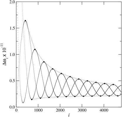
Figure 2: A plot of $\Delta\omega_{i}$, defined in the text, against $i$, showing convergence to the asymptotic value, $\Delta\omega$. The dashed lines show the least squares fit curves through the peaks and troughs of the plot of $\Delta\omega_{i}$.

Appendix D The Fourier form of the expressions for $X_{i}(\mathbf{x}),\,Y_{i}(\mathbf{x})$

We start by expanding the sine terms in $G(x,t)$ in equation (2) in the spin-orbit ODE to obtain

$$\begin{cases}\dot{x}=y,\\ \dot{y}=-\varepsilon[a(t)\cos 2x+b(t)\sin 2x]-\gamma\alpha\left(y-\omega\right)\end{cases}$$ (43)

where $a(t),\,b(t)$ are Fourier polynomials in $t$. We wish to show that, formally, we can write

$$x(t_{0}+h)=x_{0}+A_{i,0}(y_{0})+\sum_{j=1}^{\infty}\varepsilon^{j}\left[A_{i,j}(y_{0})\cos 2jx_{0}+B_{i,j}(y_{0})\sin 2jx_{0}\right]$$ (44)

where $x_{0}=x(t_{0})$, $y_{0}=y(t_{0})$ and $A_{i,j},\,B_{i,j}$ are polynomials in $y_{0}$, $h$ and the parameters in the ODE, but not $x_{0}$. We refer to this as the Fourier series form. The point we wish to make here is that the $j$-th coefficient in the expansion of $x(t_{0}+h)$ in this form always has a factor of $\varepsilon^{j}$. That is not to say that, for small $\varepsilon$, the Fourier coefficients themselves decrease exponentially with increasing $j$, because we do not prove that $A_{i,j},\,B_{i,j}$ grow more slowly than exponentially.

To show that $x(t_{0}+h)$ can be written in the form (44), we start with the Taylor series expansion

$$x(t_{0}+h)=x_{0}+hy_{0}+\sum_{i=2}^{\infty}\frac{h^{i}}{i!}y_{0}^{(i-1)},$$

where $y_{0}^{(i)}$ is the $i$-th derivative of $y(t)=\dot{x}(t)$ at $t=t_{0}$. Using the fact that the ODE (43) supplies us with a means for substituting for the first — and hence, recursively, for all — derivatives of $y$, then $y^{(i)}(t)$ can be written as a sum of terms each of which is a product of the form

$$T(t)=\nu^{\prime}p(t)y(t)^{k}c^{d-l}s^{l},$$

where $\nu^{\prime}$ is a numerical constant; $p(t)$ is a combination of $a(t)$ and $b(t)$ and their derivatives; integer $k\geq 0$; $c=\cos(2x(t)),\,s=\sin(2x(t))$; and $d\geq l\geq 0$. We wish to prove that all terms have a factor of $\varepsilon^{d}$, so that we can always write $\nu^{\prime}=\nu\varepsilon^{d}$, where $\nu$ is another constant; from this, equation (44) will follow.

Let us define the degree of the term $T$ as the integer $d$, so that the degree of $T$ is the sum of the powers of $c$ and $s$ appearing in $T$.

Differentiating $T$ with respect to $t$, we obtain

$$(\nu^{\prime})^{-1}\,\dot{T}(t)=\dot{p}y^{k}c^{d-l}s^{l}+2py^{k+1}\left[-(d-l)c^{d-l-1}s^{l+1}+lc^{d-l+1}s^{l-1}\right]+kpy^{k-1}\dot{y}c^{d-l}s^{l}.$$

As it stands, this expression consists of four terms each of degree $d$, but using (43) to replace $\dot{y}$, the last term becomes

$$kpy^{k-1}\left[-\varepsilon ac-\varepsilon bs-\gamma\alpha y+\gamma\alpha\omega\right]c^{d-l}s^{l}=-\varepsilon kpy^{k-1}\left[ac^{d-l+1}s^{l}+bc^{d-l}s^{l+1}\right]+kpy^{k-1}\gamma\alpha(-y+\omega)c^{d-l}s^{l}.$$

This expression consists of two terms of degree $d+1$, both of which are multiplied by $\varepsilon$, and two terms of degree $d$, neither of which are multiplied by $\varepsilon$. Hence, differentiation of a term of degree $d$, followed by substitution of $\dot{y}$, if present, leads to an expression of the form $\varepsilon\times[\mbox{sum of terms of degree $(d+1)$}]+[\mbox{sum of terms of degree $d$}]$. Since differentiation and substitution are the only processes by which $y^{(i)}$ is generated, by induction all terms in $y^{(i)}$ of degree $d$ have a factor of $\varepsilon^{d}$. Furthermore, any expression $c^{d-l}s^{l}$ is equal to a sum of terms of the form $\sin 2ix$, $\cos 2ix$, with $i=0,\ldots,d$; and from this, the form (44) follows.

Numerical evidence suggests that $A_{i,j}$ and $B_{i,j}$ actually decrease faster than $\varepsilon^{j}$, at least for $j=2,\,3$ — see Fig. 3.

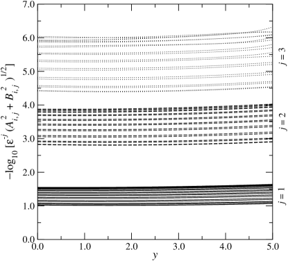
Figure 3: A logarithmic plot of $\varepsilon^{-j}\sqrt{A_{i,j}(y)^{2}+B_{i,j}(y)^{2}}$, $i=1,\ldots M=20$ and $j=1,2,3$, against $y$, where the polynomials $A_{i,j}$ and $B_{i,j}$ are defined in equation (44). Only the first three Fourier coefficients are needed to meet the error criterion explained in Sect. 3. The polynomials were computed for $\epsilon=1.2\times 10^{-4}$, $K=10^{-4}$ and $e=0.2056$. The figure shows that, for these parameters at least, $A_{i,j}$ and $B_{i,j}$ decrease faster than than $\varepsilon^{j}$ for all $i$.

References

- [Asher and Petzold (1998)] U.M. Asher and L.R. Petzold, Computer Methods for Ordinary Differential Equations and Differential-Algebraic Equations, ISBN 0-89871-412-5, SIAM, Philadelphia (1998)
- [Bartuccelli et al. (2012)] M.V. Bartuccelli, J.H.B. Deane, G. Gentile, Attractiveness of periodic orbits in parametrically forced systems with time-increasing friction, J. Math. Phys. 53, no. 10, 102703, 27 pp (2012)
- [Celletti and Chierchia (2008)] A. Celletti, L. Chierchia, Measures of basins of attraction in spin-orbit dynamics, Celestial Mech. Dynam. Astronom. 101, no. 1-2, 159–170 (2008)
- [Celletti and Chierchia (2009)] A. Celletti, L. Chierchia, Quasi-periodic attractors in celestial mechanics Arch. Ration. Mech. Anal. 191, no. 2, 311–345 (2009)
- [Celletti (2010)] A. Celletti, Stability and chaos in celestial mechanics, ISBN 978-3-540-85145-5, Springer Verlag, Berlin (2010)
- [Chang and Corliss (1980)] Y.F. Chang and G. Corliss, Ratio-like and recurrence relation test for convergence of series, J. Inst. Math. Appl. 25, 349–359 (1980)
- [Chierchia and Gallavotti (1982)] L. Chierchia, G. Gallavotti, Smooth prime integrals for quasi-integrable Hamiltonian systems, Nuovo Cimento B 67, no. 2, 277-295 (1982)
- [Coddington and Levinson (1955)] E.A. Coddington and N. Levinson, Theory of ordinary differential equations, ISBN 978-0-89874-755-3, McGraw-Hill, New York (1955)
- [Correia and Laskar (2004)] A.C.M. Correia, J. Laskar, Mercury’s capture into the 3/2 spin-orbit resonance as a result of its chaotic dynamics Nature 429, 848–850 (2004)
- [Danby (1962)] J.M.A. Danby, Fundamentals of Celestial Mechanics, Macmillan, New York (1962)
- [Gentile (2006)] G. Gentile, Diagrammatic techniques in perturbation theory, Encyclopedia of Mathematical Physics, Eds. J.-P. Françoise, G.L. Naber and T. Sh. Tsun, Elsevier, Oxford, 2, 54–60, (2006)
- [Gentile et al. (2007)] G. Gentile, M.V. Bartuccelli, J.H.B. Deane, Bifurcation curves of subharmonic solutions and Melnikov theory under degeneracies, Rev. Math. Phys. 19, no. 3, 307–348 (2007)
- [Gentile (2009)] G. Gentile, Diagrammatic methods in classical perturbation theory, Encyclopedia of Complexity and System Science, Ed. R.A. Meyers, Springer, Berlin, 2, 1932–1948 (2009)
- [Gentile (2010)] G. Gentile, Quasiperiodic motions in dynamical systems: review of a renormalization group approach, J. Math. Phys. 51, no. 1, 015207, 34 pp. (2010)
- [Goldreich and Peale (1966)] P. Goldreich, S. Peale, Spin-orbit coupling in the solar system, Astronom. J. 71, no. 6, 425–438 (1966)
- [Hairer et al. (1993)] E. Hairer, S.P. Nørsett and G. Wanner, Solving Ordinary Differential Equations I. Nonstiff problems, ISBN 978-3-540-56670-0, Second Revised Edition, Springer Series in Computational Mathematics, Springer-Verlag, Berlin and Heidelberg (1993)
- [Handscomb (1966)] D.C. Handscomb (Ed.), Methods of Numerical Approximation, Pergamon Press, Oxford (1966)
- [Jorba and Zou (2005)] À. Jorba and M. Zou, A software package for the numerical integration of ODE by means of high-order Taylor methods, Experimental Mathematics 14, pp. 99–117 (2005)
- [MacDonald (1964)] G.J.F. MacDonald, Tidal Friction, Rev. Geophys. 2, 467–541 (1964)
- [Makarov (2012)] V.V. Makarov, Conditions of passage and entrapment of terrestrial planets in spin-orbit resonances, Astrophys. J., 752, no. 1, 73 (2012)
- [Murray and Dermott (1999)] C.D. Murray and S.F. Dermott Solar System Dynamics, ISBN 0-521-57295-9, Cambridge University Press, Cambridge, UK (1999)
- [Noyelles et al. (2013)] B. Noyelles, J. Frouard, V.V. Makarov and M. Efroimsky, Spin-orbit evolution of Mercury revisited, pre-print; arXiv:1307.0136 (2013)
- [Pöschel (1982)] J. Pöschel, Integrability of Hamiltonian systems on Cantor sets, Comm. Pure Appl. Math. 35, no. 5, 653–696 (1982)
- [Press et al. (1992)] W.H. Press, S.A. Teukolsky, W.T. Vetterling and B.P. Flannery, Numerical Recipes in C, ISBN 0-521-43108-5, Cambridge University Press, Cambridge, UK (1992)
- [Saari (1970)] D. Saari, Power series solutions, Celestial Mechanics, 1, 331–342 (1970)
- [Verhulst (1990)] F. Verhulst, Nonlinear differential equations and dynamical systems, ISBN 978-3-54-050628-7, Springer, Berlin (1990)
- [Walpole et al. (1998)] R.E. Walpole, R.H. Myers and S.L. Myers, Probability and Statistics for Engineers and Scientists ISBN 0-13-840208-9, Prentice Hall, Upper Saddle River, NJ (1998)
- [Whitney (1934)] H. Whitney, Analytic extensions of differential functions defined in closed sets, Trans. Amer. Math. Soc. 36, no. 1, 63–89 (1934)
- [Williams and Efroimsky (2012)] J.G. Williams and M. Efroimsky, Bodily tides near the 1:1 spin-orbit resonance: correction to Goldreich’s dynamical model, Celestial Mech. Dynam. Astronom. 114, 387–414 (2012)
- [Yoshida (1990)] H. Yoshida, Construction of higher order symplectic integrators, Phys. Lett. A 150, 262–269 (1990)