A unified approach to linear probing hashing with buckets

Abstract.

We give a unified analysis of linear probing hashing with a general bucket size. We use both a combinatorial approach, giving exact formulas for generating functions, and a probabilistic approach, giving simple derivations of asymptotic results. Both approaches complement nicely, and give a good insight in the relation between linear probing and random walks. A key methodological contribution, at the core of Analytic Combinatorics, is the use of the symbolic method (based on $q$-calculus) to directly derive the generating functions to analyze.

1. Motivation

Linear probing hashing, defined below, is certainly the simplest “in place” hashing algorithm [25].

• A table of length $m$, $T[1\,.\,.\,m]$, with buckets of size $b$ is set up, as well as a hash function $h$ that maps keys from some domain to the interval $[1\,.\,.\,m]$ of table addresses. A collection of $n$ keys with $n\leqslant bm$ are entered sequentially into the table according to the following rule: Each key $x$ is placed at the first bucket that is not full starting from $h(x)$ in cyclic order, namely the first of $h(x),h(x)+1,\ldots,m,1,2,\ldots,h(x)-1$.

In [26] Knuth motivates his paper in the following way: “The purpose of this note is to exhibit a surprisingly simple solution to a problem that appears in a recent book by Sedgewick and Flajolet [36]:

Exercise 8.39  Use the symbolic method to derive the EGF of the number of probes required by linear probing in a successful search, for fixed $M$.”

Moreover, at the end of the paper in his personal remarks he declares: “None of the methods available in 1962 were powerful enough to deduce the expected square displacement, much less the higher moments, so it is an even greater pleasure to be able to derive such results today from other work that has enriched the field of combinatorial mathematics during a period of 35 years.” In this sense, he is talking about the powerful methods based on Analytic Combinatorics that has been developed for the last decades, and are presented in [16].

In this paper we present in a unified way the analysis of several random variables related with linear probing hashing with buckets, giving explicit and exact trivariate generating functions in the combinatorial model, together with generating functions in the asymptotic Poisson model that provide limit results, and relations between the two types of results. We consider also the parking problem version, where there is no wrapping around and overflow may occur from the last bucket. Linear probing has been shown to have strong connections with several important problems (see [26; 15; 7] and the references therein). The derivations in the asymptotic Poisson model are probabilistic and use heavily the relation between random walks and the profile of the table. Moreover, the derivations in the combinatorial model are based in combinatorial specifications that directly translate into multivariate generating functions. As far as we know, this is the first unified presentation of the analysis of linear probing hashing with buckets based on Analytic Combinatorics (“if you can specify it, you can analyze it”).

We will see that results can easily be translated between the exact combinatorial model and the asymptotic Poisson model. Nevertheless, we feel that it is important to present independently derivations for the two models, since the methodologies complement very nicely. Moreover, they heavily rely in the deep relations between linear probing and other combinatorial problems like random walks, and the power of Analytic Combinatorics.

The derivations based on Analytic Combinatorics heavily rely on a lecture presented by Flajolet whose notes can be accessed in [12]. Since these ideas have only been partially published in the context of the analysis of hashing in [16], we briefly present here some constructions that lead to $q$-analogs of their corresponding multivariate generating functions.

2. Some previous work

The main application of linear probing is to retrieve information in secondary storage devices when the load factor is not too high, as first proposed by Peterson [33]. One reason for the use of linear probing is that it preserves locality of reference between successive probes, thus avoiding long seeks [29].

The first published analysis of linear probing was done by Konheim and Weiss [28]. In addition, this problem also has a special historical value since the first analysis of algorithms ever performed by D. Knuth [24] was that of linear probing hashing. As Knuth indicates in many of his writings, the problem has had a strong influence on his scientific carreer. Moreover, the construction cost to fill a linear probing hash table connects to a wealth of interesting combinatorial and analytic problems. More specifically, the Airy distribution that surfaces as a limit law in this construction cost is also present in random trees (inversions and path length), random graphs (the complexity or excess parameter), and in random walks (area), as well as in Brownian motion (Brownian excursion area) [26; 15; 22].

Operating primarily in the context of double hashing, several authors [4; 1; 18] observed that a collision could be resolved in favor of any of the keys involved, and used this additional degree of freedom to decrease the expected search time in the table. We obtain the standard scheme by letting the incoming key probe its next location. So, we may see this standard policy as a first-come-first-served (FCFS) heuristic. Later Celis, Larson and Munro [5; 6] were the first to observe that collisions could be resolved having variance reduction as a goal. They defined the Robin Hood heuristic, in which each collision occurring on each insertion is resolved in favor of the key that is farthest away from its home location. Later, Poblete and Munro [34] defined the last-come-first-served (LCFS) heuristic, where collisions are resolved in favor of the incoming key, and others are moved ahead one position in their probe sequences. These strategies do not look ahead in the probe sequence, since the decision is made before any of the keys probes its next location. As a consequence, they do not improve the average search cost, although the variance of this random variable is different for each strategy.

For the FCFS heuristic, if $A_{m,n}$ denotes the number of probes in a successful search in a hash table of size $m$ with $n$ keys (assuming all keys in the table are equally likely to be searched), and if we assume that the hash function $h$ takes all the values in $0\ldots m-1$ with equal probabilities, then we know from [25; 17]

$${\operatorname{\mathbb{E}{}}}[A_{m,n}] =\frac{1}{2}(1+Q_{0}(m,n-1)),$$ (2.1)

$${\operatorname{Var}}[A_{m,n}] =\frac{1}{3}Q_{2}(m,n-1)-\frac{1}{4}Q_{0}(m,n-1)^{2}-\frac{1}{12}.$$ (2.2)

where

$$Q_{r}(m,n)=\sum_{k=0}^{n}\binom{k+r}{k}\frac{n^{\underline{k}}}{m^{k}}$$

and $n^{\underline{k}}$ defined as $n^{\underline{k}}=n(n-1)\ldots(n-k+1)$ for real $n$ and integer $k\geq 0$ is the $k$:th falling factorial power of $n$. The function $Q_{0}(m,n)$ is also known as Ramanujan’s $Q$-function [13].

For a table with $n=\alpha m$ keys, and fixed $\alpha<1$ and $n,m\rightarrow\infty$, these quantities depend (essentially) only on $\alpha$:

$${\operatorname{\mathbb{E}{}}}[A_{m,\alpha m}] =\frac{1}{2}\left(1+\frac{1}{1-\alpha}\right)-\frac{1}{2(1-\alpha)^{3}m}+O\left(\frac{1}{m^{2}}\right),$$

$${\operatorname{Var}}[A_{m,\alpha m}] =\frac{1}{3(1-\alpha)^{3}}-\frac{1}{4(1-\alpha)^{2}}-\frac{1}{12}-\frac{1+3\alpha}{2(1-\alpha)^{5}m}+O\left(\frac{1}{m^{2}}\right).$$

For a full table, these approximations are useless, but the properties of the $Q$ functions can be used to obtain the following expressions, reproved in Corollary 12.5,

$${\operatorname{\mathbb{E}{}}}[A_{m,m}] =\frac{\sqrt{2\pi m}}{4}+\frac{1}{3}+\frac{1}{48}\sqrt{\frac{2\pi}{m}}+O\left(\frac{1}{m}\right),$$ (2.3)

$${\operatorname{Var}}[A_{m,m}] =\frac{\sqrt{2\pi m^{3}}}{12}+\left(\frac{1}{9}-\frac{\pi}{8}\right)m+\frac{13\sqrt{2\pi m}}{144}-\frac{47}{405}-\frac{\pi}{48}+O\left(\frac{1}{\sqrt{m}}\right).$$ (2.4)

As it can be seen the variance is very high, and as a consequence the Robin Hood and LCFS heuristics are important in this regard. It is proven in [5; 6] that Robin Hood achieves the minimum variance among all the heuristics that do not look ahead at the future, and that LCFS has an asymptotically optimal variance [35]. This problem appears in the simulations presented in Section 13, and as a consequence even though the expected values that we present are very informative, there is still a disagreement with the experimental results.

Moreover, in [21] and [39], a distributional analysis for the FCFS, LCFS and Robin Hood heuristic is presented. These results consider a hash table with buckets of size 1. However, very little is known when we have tables with buckets of size $b$.

In [3], Blake and Konheim studied the asymptotic behavior of the expected cost of successful searches as the number of keys and buckets tend to infinity with their ratio remaining constant. Mendelson [30] derived exact formulae for the same expected cost, but only solved them numerically. These papers consider the FCFS heuristic. Moreover, in [41] an exact analysis of a linear probing hashing scheme with buckets of size $b$ (working with the Robin Hood heuristic) is presented. The first complete distributional analysis of the Robin Hood heuristic with buckets of size $b$ is presented in [40], where an independent analysis of the parking problem presented in [37] is also proposed.

In the present paper we consider an arbitrary bucket size $b\geqslant 1$. The special case $b=1$ has been studied in many previous works. In this case, many of our results reduce to known results, see e.g. [21] and [39] and the references given there.

3. Some notation

We study tables with $m$ buckets of size $b$ and $n$ keys, where $b\geqslant 1$ is a constant. We often consider limits as $m,n\to\infty$ with $n/bm\to\alpha$ with $\alpha\in(0,1)$. We consider also the Poisson model with $n\sim\operatorname{Po}(\alpha bm)$, and thus $\operatorname{Po}(b\alpha)$ keys hashed to each bucket; in this model we can also take $m=\infty$ which gives a natural limit object, see Sections 6–7.

A cluster or block is a (maximal) sequence of full buckets ended by a non-full one. An almost full table is a table consisting of a single cluster.

The tree function [16, p. 127] is defined by

$$T(z):=\sum_{n=1}^{\infty}\frac{n^{n-1}}{n!}z^{n},$$ (3.1)

which converges for $|z|\leqslant e^{-1}$; $T(z)$ satisfies $T(e^{-1})=1$ and

$$z=T(z)e^{-T(z)}.$$ (3.2)

In particular, note that (3.2) implies that $T(z)$ is injective on $|z|\leqslant e^{-1}$. Recall also the well-known formula (easily obtained by taking the logarithmic derivative of (3.2))

$$T^{\prime}(z)=\frac{T(z)}{z(1-T(z))}.$$ (3.3)

(The tree function is related to the Lambert $W$-function $W(z)$ [31, §4.13] by $T(z)=-W(-z)$.)

Let $\omega=\omega_{b}:=e^{2\pi\mathrm{i}/b}$ be a primitive $b$:th unit root.

For $\alpha$ with $0<\alpha<1$, we define

$$\zeta_{\ell}(q)=\zeta_{\ell}(q;\alpha):=T\bigl{(}\omega^{\ell}\alpha e^{-\alpha}q^{1/b}\bigr{)}/\alpha$$ (3.4)

and

$$\zeta_{\ell}:=\zeta_{\ell}(1)=T\bigl{(}\omega^{\ell}\alpha e^{-\alpha}\bigr{)}/\alpha.$$ (3.5)

Note that

$$\zeta_{0}=T\bigl{(}\alpha e^{-\alpha}\bigr{)}/\alpha=1,$$ (3.6)

cf. (3.2) (with $z=\alpha e^{-\alpha}$). We note the following properties of these numbers.

Lemma 3.1.

Let $0<\alpha<1$. Then (3.4) defines $b$ numbers $\zeta_{\ell}(q)$, $\ell=0,\dots,b-1$, for every $q$ with $|q|\leqslant R:=(e^{\alpha-1}/\alpha)^{b}>1$. If furthermore $q\neq 0$, then these $b$ numbers are distinct.

If $|q|\leqslant 1$, then the $b$ numbers $\zeta_{\ell}(q)$, $\ell=0,\dots,b-1$, satisfy $|\zeta_{\ell}(q)|\leqslant 1$, and they are the $b$ roots in the unit disc of

$$\zeta^{b}=e^{\alpha b(\zeta-1)}q.$$ (3.7)

Proof.

Note first that

$$|\alpha e^{-\alpha}\omega^{\ell}q^{1/b}|\leqslant e^{-1}$$ (3.8)

is equivalent to

$$|q|\leqslant R:=(e^{\alpha-1}/\alpha)^{b}>1,$$ (3.9)

so all $\zeta_{\ell}(q)$ are defined for $|q|\leqslant R$. If also $q\neq 0$, then $\zeta_{0}(q),\dots,\zeta_{b-1}(q)$ are distinct, because $T$ is injective by (3.2). Furthermore, for $|q|\leqslant 1$, using (3.4), the fact that (3.1) has positive coefficients, and (3.6),

$$|\zeta_{\ell}(q)|\leqslant\alpha^{-1}T\bigl{(}\alpha e^{-\alpha}\bigr{)}=1.$$ (3.10)

Moreover, (3.4) and (3.2) imply

$$\alpha\zeta_{\ell}(q)e^{-\alpha\zeta_{\ell}(q)}=\alpha e^{-\alpha}\omega^{\ell}q^{1/b}$$ (3.11)

which by taking the $b$:th powers yields (3.7). Since the derivative of $e^{\alpha b(r-1)}-r^{b}$ at $r=1$ is $\alpha b-b<0$, we can find $r>1$ such that $e^{\alpha b(r-1)}<r^{b}$, and then Rouché’s theorem shows that, for any $q$ with $|q|\leqslant 1$, $\zeta^{b}-e^{\alpha b(\zeta-1)}q$ has exactly $b$ roots in $|\zeta|<r$; thus, the $b$ roots $\zeta_{0}(q),\dots,\zeta_{b-1}(q)$ are the only roots of (3.7) in $|\zeta|<r$. (The case $q=0$ is trivial.) ∎

Remark 3.2.

In order to define an individual $\zeta_{\ell}(q)$, we have to fix a choice of $q^{1/b}$ in (3.4). It is thus impossible to define each $\zeta_{\ell}(q)$ as a continuous function in the entire unit disc; they rather are different branches of a single, multivalued, function, with a branch point at $0$. Nevertheless, it is only the collection of all of them together that matters, for example in (10.8), and this collection is uniquely defined.

We denote convergence in distribution of random variables by $\overset{\mathrm{d}}{\longrightarrow}$.

4. Combinatorial characterization of linear probing

As a combinatorial object, a non-full linear probing hash table is a sequence of almost full tables (or clusters) [26; 15; 40]. As a consequence, any random variable related with the table itself (like block lengths, or the overflow in the parking problem) or with a random key (like its search cost) can be studied in a cluster (that we may assume to be the last one in the sequence), and then use the sequence construction. Figure 1 presents an example of such a decomposition.

We briefly recall here some of the definitions presented in [3; 40]. Let $F_{bi+d}$ be the number of ways to construct an almost full table of length $i+1$ and size $bi+d$ (that is, there are $b-d$ empty slots in the last bucket). Define also

$$F_{d}(u):=\sum_{i\geq 0}F_{bi+d}\frac{u^{bi+d}}{(bi+d)!}, N_{d}(z,w):=\sum_{s=0}^{b-1-d}w^{b-s}F_{s}(zw),\quad 0\leq d\leq b-1.$$ (4.1)

In this setting $N_{d}(z,w)$ is the generating function for the number of almost full tables with more than $d$ empty locations in the last bucket. More specifically $N_{0}(z,w)$ is the generating function for the number of all the almost full tables. (Our generating functions use the weight $w^{bm}z^{n}/n!$ for a table of length $m$ and $n$ keys; they are thus exponential generating functions in $n$ and ordinary generating functions in $m$.) We present below some basic identities.

Lemma 4.1.

$$F(bz,x) :=\sum_{d=0}^{b-1}F_{d}(bz)x^{d}=x^{b}-\prod_{j=0}^{b-1}\left(x-\frac{T(\omega^{j}z)}{z}\right),$$ (4.2)

$$\sum_{d=0}^{b-1}N_{d}(bz,w)x^{d} =\frac{\displaystyle{\prod_{j=0}^{b-1}\left(1-x\frac{T(\omega^{j}zw)}{z}\right)-\prod_{j=0}^{b-1}\left(1-\frac{T(\omega^{j}zw)}{z}\right)}}{1-x},$$ (4.3)

$$\sum_{d=0}^{b-1}N_{d}(b\alpha,e^{-\alpha})x^{d} =\prod_{j=1}^{b-1}\left(1-x\frac{T(\omega^{j}\alpha e^{-\alpha})}{\alpha}\right).$$ (4.4)

Proof.

Equation (4.2) can be derived from Lemma 2.3 in [3].

Moreover, from equation (4.1),

$$\sum_{d=0}^{b-1}N_{d}(bz,w)x^{d} =\sum_{d=0}^{b-1}x^{d}\sum_{s=0}^{b-1-d}w^{b-s}F_{s}(bzw)=\sum_{s=0}^{b-1}w^{b-s}F_{s}(bzw)\sum_{d=0}^{b-1-s}x^{d}$$

$$=\frac{\displaystyle{\sum_{s=0}^{b-1}w^{b-s}F_{s}(bzw)-\sum_{s=0}^{b-1}(wx)^{b-s}F_{s}(bzw)}}{1-x}$$

$$=\frac{\displaystyle{w^{b}F\left(bzw,\frac{1}{w}\right)-(wx)^{b}F\left(bzw,\frac{1}{wx}\right)}}{1-x}.$$

Then (4.3) follows from (4.2).

Finally (4.4) follows from (4.3), and since $T(\alpha e^{-\alpha})=\alpha$ the factor for $j=0$ cancels the second product, and gives the factor $(1-x)$ in the first one that cancels with the denominator. ∎

Corollary 4.2.

$$N_{d}(bz,w)=[x^{d}]\frac{\displaystyle{\prod_{j=0}^{b-1}\left(1-x\frac{T(\omega^{j}zw)}{z}\right)-\prod_{j=0}^{b-1}\left(1-\frac{T(\omega^{j}zw)}{z}\right)}}{1-x},$$ (4.5)

and more specifically (formula (3.8) in [3]),

$$N_{0}(bz,w)=1-\prod_{j=0}^{b-1}\left(1-\frac{T(\omega^{j}zw)}{z}\right).$$ (4.6)

Moreover (Lemma 5 in [40]),

$$N_{d}(b\alpha,e^{-\alpha})=\left[x^{d}\right]\prod_{j=1}^{b-1}\left(1-x\frac{T(\omega^{j}\alpha e^{-\alpha})}{\alpha}\right).$$ (4.7)

Let also $Q_{m,n,d}$, for $0\leqslant d\leqslant b-1$, be the number of ways of inserting $n$ keys into a table with $m$ buckets of size $b$, so that a given (say the last) bucket of the table contains more than $d$ empty slots. (We include the empty table, and define $Q_{0,0,d}=1$.) In this setting, by a direct application of the sequence construction as presented in [16] (sequence of almost full tables) we derive a result presented in [3]:

$$\Lambda_{0}(bz,w):=\sum_{m\geq 0}\sum_{n\geq 0}Q_{m,n,0}\frac{(bz)^{n}}{n!}w^{bm}=\frac{1}{1-N_{0}(bz,w)}=\frac{1}{\prod_{j=0}^{b-1}\left(1-\frac{T(\omega^{j}zw)}{z}\right)},$$ (4.8)

where $\Lambda_{0}(bz,w)$ is the generating function for the number of ways to construct hash tables such that their last bucket is not full, and more generally

$$\Lambda_{d}(bz,w):=\sum_{m\geq 0}\sum_{n\geq 0}Q_{m,n,d}\frac{(bz)^{n}}{n!}w^{bm}=1+\frac{N_{d}(bz,w)}{1-N_{0}(bz,w)}.$$ (4.9)

Moreover $O_{d}(bz,w)$, the generating function for the number of ways to construct hash tables such that their last bucket has exactly $d\leqslant b-1$ keys, is

$$O_{d}(bz,w):=\frac{F_{d}(bzw)w^{b-d}}{1-N_{0}(bz,w)}.$$ (4.10)

   

Figure 1. A decomposition for $b=3$ and $d=2$.

Consider a hash table of length $m$ and $n$ keys, where collisions are resolved by linear probing. Let $P$ be a non-negative integer-valued property (e.g. cost of a successful search or block length), related with the last cluster of the sequence, or with a random key inside it. Let $p_{bi+d}(q)$ be the probability generating function of $P$ calculated in the cluster of length $i+1$ and with $bi+d$ keys (as presented in Figure 1). We may express $p_{m,n}(q)$, the generating function of $P$ for a table of length $m$ and $n$ keys with at least one empty spot in the last bucket, as the sum of the conditional probabilities:

$$p_{m,n}(q)=\sum_{d=0}^{b-1}\sum_{i\geqslant 0}\#\{\text{tables where last cluster has size $i+1$ and $bi+d$ keys}\}~{}p_{bi+d}(q).$$

There are $Q_{m-i-1,n-bi-d,0}$ ways to insert $n-bi-d$ keys in the leftmost hash table of length $m-i-1$, leaving their rightmost bucket not full. Moreover, there are $F_{bi+d}$ ways to insert $bi+d$ keys in the almost full table of length $i+1$. Furthermore, there are $\binom{n}{bi+d}$ ways to choose which $bi+d$ keys go to the last cluster. Therefore,

$$p_{m,n}(q)=\sum_{d=0}^{b-1}\sum_{i\geq 0}\binom{n}{bi+d}{Q_{m-i-1,n-bi-d,0}~{}F_{bi+d}}~{}~{}p_{bi+d}(q).$$

Then, the trivariate generating function for $p_{m,n}(q)$ is

$$P(z,w,q) :=\sum_{m,n\geq 0}p_{m,n}(q)~{}w^{bm}\frac{z^{n}}{n!}=\Lambda_{0}(z,w)\hat{N}_{0}(z,w,q),$$ (4.11)

with

$$\hat{N}_{0}(z,w,q) :=\sum_{i\geq 0}w^{b(i+1)}\sum_{d=0}^{b-1}F_{bi+d}~{}\frac{z^{bi+d}}{(bi+d)!}~{}p_{bi+d}(q),$$ (4.12)

which could be directly derived with the sequence construction [16]. In this setting, $w$ marks the total capacity ($b(i+1)$) while $z$ marks the number of keys in the table ($bi+d$ with $0\leq d<b$). Equation (4.11) can be interpreted as follows: to analyze a property in a linear probing hash table, do the analysis in an almost full table (giving the factor $\hat{N}_{0}(z,w,q)$), and then use the sequence construction (giving the factor $\Lambda_{0}(z,w)$).

Notice that, as expected, $\hat{N}_{0}(z,w,1)=N_{0}(z,w)$ and $P(z,w,1)=\Lambda_{0}(z,w)-1$, since we consider only $m\geq 1$ (we have a last, non-filled bucket).

Remark 4.3.

We have here, for simplicity, assumed that each $p_{bi+d}(q)$ is a probability generating function, corresponding to a single property $P$ of the last cluster. However, the argument above generalizes to the case when $p_{bi+d}(q)$ is a generating function corresponding to several values of a property $P$ for each cluster; (4.11) and (4.12) still hold, although we no longer have $p_{bi+d}(1)=1$ and thus not $\hat{N}_{0}(z,w,1)=N_{0}(z,w)$ (in general). We use this in Sections 11 and 12.

4.1. The Poisson Transform

There are two standard models that are extensively used in the analysis of hashing algorithms: the exact filling model and the Poisson filling model. Under the exact model, we have a fixed number of keys, $n$, that are distributed among $m$ buckets of size $b$, and all $m^{n}$ possible arrangements are equally likely to occur.

Under the Poisson model, we assume that each location receives a number of keys that is Poisson distributed with parameter $b\alpha$ (with $0\leq\alpha<1$) , and is independent of the number of keys going elsewhere. This implies that the total number of keys, $N$, is itself a Poisson distributed random variable with parameter $b\alpha m$:

$$\Pr\left[N=n\right]=\frac{e^{-b\alpha m}(b\alpha m)^{n}}{n!},\qquad n\ =\ 0,1,\ldots$$

(For finite $m$, there is an exponentially small probability that $N>bm$; this possibility can usually be ignored in the limit $m,n\to\infty$. For completeness we assume either that we consider the parking problem where overflow may occur, or that we make some special definition when $N>bm$. See also the infinite Poisson model in Section 7, where this problem disappears.) This model was first considered in the analysis of hashing, for a somewhat different problem, by Fagin et al [10] in 1979.

The results obtained under the Poisson filling model can be interpreted as an approximation of those one would obtain under the exact filling model when $n=b\alpha m$. For most situations and applications, this approximation is satisfactory for large $m$ and $n$. (However, it cannot be used when we have a full, or almost full, table, so $\alpha$ is very close to 1.) We give a detailed statement of one general limit theorem (Theorem 7.4) later, but give a brief sketch here. We begin with some algebraic identities.

Consider a hash table of size $m$ with $n$ keys, in which conflicts are resolved by open addressing using some heuristic. Let the variable $P$ be a non-negative integer-valued property of the table (e.g. the block length of a random cluster), or of a random key of the table (e.g., the cost of a successful search), and let $f_{m,n}$ be the result of applying a linear operator $f$ (e.g., an expected value) to the probability generating function of $P$ for the exact filling model. Let ${\bf{P}}_{m}[f_{m,n};b\alpha]$ be the result of applying the same linear operator $f$ to the probability generating function of $P$ computed using the Poisson filling model. Then

$${\bf{P}}_{m}[f_{m,n};b\alpha] =\sum_{n\geq 0}\Pr\left[N=n\right]f_{m,n}=e^{-bm\alpha}\sum_{n\geq 0}\frac{(bm\alpha)^{n}}{n!}f_{m,n}.$$ (4.13)

In this context, ${\bf{P}}_{m}[f_{m,n};b\alpha]$ is called the Poisson transform of $f_{m,n}$.

In particular, let $P_{m,n}(q)$ be the generating function of a variable $P$ in a hash table of size $m$ with $n$ keys, and let $p_{m,n}(q)=P_{m,n}(q)/m^{n}$ be the corresponding probability generating function of $P$ regarded as a random variable (with all $m^{n}$ tables equally likely). Define the trivariate generating function

$$P(z,w,q):=\sum_{m\geq 0}w^{bm}\sum_{n\geq 0}{P_{m,n}(q)}\frac{z^{n}}{n!}=\sum_{m\geq 0}w^{bm}\sum_{n\geq 0}p_{m,n}(q)\frac{(mz)^{n}}{n!}.$$

Then, for a fixed $0\leq\alpha<1$, using (4.13),

$$\begin{split}P(b\alpha,y^{1/b}e^{-\alpha},q)&=\sum_{m\geq 0}y^{m}\left(e^{-bm\alpha}\sum_{n\geq 0}{p_{m,n}(q)}\frac{(bm\alpha)^{n}}{n!}\right)\\ &=\sum_{m\geq 0}y^{m}{\bf P}_{m}\left[{p_{m,n}(q)};b\alpha\right].\end{split}$$ (4.14)

In other words, $P(b\alpha,y^{1/b}e^{-\alpha},q)$ is the generating function of ${\bf P}_{m}[p_{m,n}(q);b\alpha]$.

Asymptotic results for the probability generating function in the Poisson model, can thus be found by singularity analysis [14; 16] from $P(b\alpha,y^{1/b}e^{-\alpha},q)$. In our problems, the dominant singularity is a simple pole at $y=1$. Furthermore, asymptotic results for the exact model can be found by de-Poissonization; we give a probabilistic proof of one such result in Theorem 7.4(i).

The same formulas without the variable $q$ hold if $P_{m,n}$ is the number of hash tables with a certain Boolean property, and $p_{m,n}=P_{m,n}/m^{n}$ is the corresponding probability that a random hash table has this property. In this case, the trivariate generating function (4.14) is replaced by the bivariate

$$\begin{split}P(b\alpha,y^{1/b}e^{-\alpha})&=\sum_{m\geq 0}y^{m}e^{-bm\alpha}\sum_{n\geq 0}{p_{m,n}}\frac{(bm\alpha)^{n}}{n!}.\end{split}$$ (4.15)

For example, from equation (4.8), $\Lambda_{0}(b\alpha,y^{1/b}e^{-\alpha})$ has a dominant simple pole at $y=1$ originated by the factor with $j=0$, since $T(\alpha e^{-\alpha})/\alpha=1$. More precisely, using (3.3),

$$\frac{1}{1-\frac{T\left(y^{1/b}\alpha e^{-\alpha}\right)}{\alpha}}\quad^{~{}\displaystyle{\sim}}_{y\to 1}~{}\frac{b(1-\alpha)}{1-y}.$$

and the residue of $\Lambda_{0}(b\alpha,y^{1/b}e^{-\alpha})$ at $y=1$ is

$$T_{0}(b\alpha):=\frac{b(1-\alpha)}{\prod_{j=1}^{b-1}\left(1-\frac{T(\omega^{j}\alpha e^{-\alpha})}{\alpha}\right)}.$$ (4.16)

Then the following result presented in ([3; 40]) is rederived, see also Theorem 7.4(ii)(iii):

$$\lim_{m\to\infty}{\mathbf{P}}_{m}[Q_{m,n,0}/m^{n};b\alpha]=T_{0}(b\alpha).$$ (4.17)

Moreover, from (4.11) we similarly obtain, for a property $P$,

$$\lim_{m\to\infty}\mathbf{P}_{m}[p_{m,n}(q)/m^{n};b\alpha] =T_{0}(b\alpha)\hat{N}_{0}(b\alpha,e^{-\alpha},q).$$ (4.18)

By de-Poissonization, we further find asymptotics for $Q_{m,n,0}$ and (for suitable properties $P$) $p_{m,n}(q)$, see Theorem 7.4(i).

Even though by equations (4.14) and (4.18) the results in the exact model can be directly translated into their counterpart in the Poisson model, in this paper we present derivations for both approaches. We feel this is very important to present a unified point of view of the problem. Furthermore, the deriviations made in each model are also unified. For the exact model, a direct approach using the symbolic method and the powerful tools from Analytic Combinatorics [16] is presented, while for the Poisson model, a unified approach using random walks is used. Presenting both related but independently derived analyses, helps in the better understanding of the combinatorial, analytic and probabilistic properties of linear probing.

5. A $q$-calculus to specify random variables

All the generating functions in this paper are exponential in $n$ and ordinary in $m$. Moreover, the variable $q$ marks the value of the random variable at hand. As a consequence all the labelled constructions in [16] and their respective translation into EGF can be used. However, to specify the combinatorial properties related with the analysis of linear probing hashing, new constructions have to be added. These ideas have been presented by Flajolet in [12], but they do not seem to have been published in the context of hashing. As a consequence, we briefly summarize them in this section.

Marking a position $\mapsto$ $\partial_{w}$	$C_{bn+d}=(n+1)A_{bn+d}$
$\mathcal{C}=\operatorname{Pos}(\mathcal{A}$)	$C(z,w)=\frac{w}{b}\frac{\partial}{\partial w}(A(z,w))$
Adding a key $\mapsto$ $\int$	$C_{bn+d}=A_{{bn+d}-1}$
$\mathcal{C}=\operatorname{Add}(\mathcal{A}$)	$C(z,w)=\int_{0}^{z}A(u,w)du$
Bucketing $\mapsto$ $\exp$	$C_{m,n}=\delta(m,1)$
$\mathcal{C}=\operatorname{Bucket}(\mathcal{Z}$)	$C(z,w)=w^{b}\exp(z)$
Marking a key $\mapsto$ $\partial_{z}$	$C_{m,n}=nA_{m,n}$
$\mathcal{C}=\operatorname{Mark}(\mathcal{A}$)	$C(z,w)=z\frac{\partial}{\partial z}A(z,w)$

Figure 2. Constructions used in hashing

We first concentrate in counting generating functions ($q=1$), and we generalize these constructions in Section 5.1 for distributional results where their $q$-analogue counterparts are presented. Figure 2 presents a list of combinatorial constructions used in hashing and their corresponding translation into EGF, where $\mathcal{Z}$ is an atomic class comprising a single key of size 1. We motivate these constructions that are specifically defined for this analysis.

Because of the sequence interpretation of linear probing, insertions are done in an almost full table with $n+1$ buckets of size $b$ (total capacity $b(n+1)$) and $bn+d$ keys. As it is seen in (4.12) in $\hat{N}_{0}(z,w,q)$ the variable $w$ marks the total capacity, while $z$ marks the number of keys. So, in this context all the generating functions to be used for the first two constructions have the form

$$A(z,w)=\sum_{n\geq 0}w^{b(n+1)}.\sum_{d=0}^{b-1}A_{bn+d}~{}\frac{z^{bn+d}}{(bn+d)!}.$$

To help in fixing ideas, we may think (as an analogue with equation (4.12)) that $A_{bn+d}=F_{bn+d}~{}p_{bn+d}(1)$.

To insert a key, a position is first chosen, and then the key is inserted. Both actions can be formally specified using the symbolic method.

• Marking a position.

  Given an almost full table with $n+1$ buckets (the last one with $d$ keys, $0\leq d<b$), a new key can hash in $n+1$ different places. As a consequence, we have the counting relation $C_{bn+d}=(n+1)A_{bn+d}$, leading to the $\partial_{w}$ relation in their respective multivariate generating functions.

  Notice that the key has not been inserted yet, only a position is chosen, and so the total number of keys in the table does not change.

• Adding a key.

  Once a position is chosen, then a key is added. In this setting $C_{bn+d}=A_{bn+d-1}$, leading to the $\int$ relation. No further calculations are needed, since it only specifies that the number of keys has been increased by 1 (all the other calculations were done when marking the position).

Other constructions are also useful to analyze linear probing hashing.

• Bucketing.

  When considering a single bucket, it has capacity $b$, giving the factor $w^{b}$ in the generating function. Moreover, for each $n$, there is only one way to hash $n$ keys in this bucket (all these key have this hash position). Since the generating functions are exponential in $n$, this gives the factor $e^{z}$ (reflecting the fact that $C_{m,n}=1$ for $n\geq 0$ and $m=1$ since there is only one bucket). In this context $\delta$ is the Dirac’s $\delta$ function ($\delta(a,b)=1$ if $a=b$ and $0$ otherwise).

  This construction is used for general hash tables with $m$ buckets and $n$ keys (not necessarily almost full) in Sections 8 and 9.

• Marking a key.

  In some cases, we need to choose a key among $n$ keys that hash to some specific location. The $q$-analogue of this construction is used in Section 9. The counting relation $C_{m,n}=nA_{m,n}$ leads to the $\partial_{z}$ relation in their respective multivariate generating functions.

5.1. The $q$-calculus.

In an almost full table with $n+1$ buckets, there are $n+1$ places where a new key can hash. However, if a distributional analysis is done, its displacement depends on the place where it has hashed: it is $i$ if the key hashes to bucket $n+1-i$ with $1\leq i\leq n+1$. In this context, to keep track of the distribution of random variables (e.g. the displacement of a new inserted key), we need generalizations of the constructions above that belong to the area of $q$-calculus (equations (5.2) and (5.3)).

The same happens to the $\operatorname{Mark}$ construction We rank the $n$ keys by the labels $0,\dots,n-1$ (in arbitrary order), and give the key with label $k$ the weight $q^{k}$ (equations (5.4) and (5.5)).

We present below some of these translations, where the variable $q$ marks the value of the random variable at hand. Moments result from using the operators $\partial_{q}$ (differentiation w.r.t. $q$) and $\mathsf{U}_{q}$ (setting $q=1$).

$$n \mapsto[n]:=1+q+q^{2}+\ldots+q^{n-1}=\frac{1-q^{n}}{1-q},$$ (5.1)

$$\sum_{n\geq 0}(n+1)w^{b(n+1)} \cdot\sum_{d=0}^{b-1}A_{bn+d}~{}\frac{z^{bn+d}}{(bn+d)!}$$

$$\mapsto\sum_{n\geq 0}[n+1]w^{b(n+1)}\cdot\sum_{d=0}^{b-1}A_{bn+d}(q)~{}\frac{z^{bn+d}}{(bn+d)!},$$ (5.2)

$$\frac{w}{b}\frac{\partial}{\partial w}A(z,w) \mapsto\mathsf{H}[A(z,w)]:=\frac{A(z,w)-A(z,wq^{\frac{1}{b}})}{1-q},$$ (5.3)

$$\sum_{m\geq 0}w^{m}\cdot\sum_{n\geq 0}nA_{m,n}~{}\frac{z^{n}}{n!} \mapsto\sum_{m\geq 0}w^{m}\cdot\sum_{n\geq 0}[n]A_{m,n}(q)~{}\frac{z^{n}}{n!},$$ (5.4)

$$z\frac{\partial}{\partial z}A(z,w) \mapsto\hat{\mathsf{H}}[A(z,w)]:=\frac{A(z,w)-A(qz,w)}{1-q}.$$ (5.5)

6. Probabilistic method: finite and infinite hash tables

In general, consider a hash table, with locations (“buckets”) each having capacity $b$; we suppose that the buckets are labelled by $i\in\mathfrak{T}$, for a suitable index set $\mathfrak{T}$. Let for each bucket $i\in\mathfrak{T}$, $X_{i}$ be the number of keys that have hash address $i$, and thus first try bucket $i$. We are mainly interested in the case when the $X_{i}$ are random, but in this section $X_{i}$ can be any (deterministic or random) non-negative integers; we consider the random case further in the next section.

Moreover, let $H_{i}$ be the total number of keys that try bucket $i$ and let $Q_{i}$ be the overflow from bucket $i$, i.e., the number of keys that try bucket $i$ but fail to find room and thus are transferred to the next bucket. We call the sequence $H_{i}$, $i\in\mathfrak{T}$, the profile of the hash table. (We will see that many quantities of interest are determine by the profile.) These definitions yield the equations

$$H_{i} =X_{i}+Q_{i-1},$$ (6.1)

$$Q_{i} =(H_{i}-b)_{+}.$$ (6.2)

The final number of keys stored in bucket $i$ is $Y_{i}:=H_{i}\wedge b:=\min(H_{i},b)$; in particular, the bucket is full if and only if $H_{i}\geqslant b$.

Remark 6.1.

The equations (6.1)–(6.2) are the same as in queuing theory, with $Q_{i}$ the queuing process generated by the random variables $X_{i}-b$, see [11, Section VI.9, in particular Example (c)].

Standard hashing is when the index set $\mathfrak{T}$ is the cyclic group $\mathbb{Z}_{m}$. Another standard case is the parking problem, where $\mathfrak{T}$ is an interval $\{1,\dots,m\}$ for some integer $m$; in this case the $Q_{m}$ keys that try the last bucket but fail to find room there are lost (overflow), and (6.1)–(6.2) use the initial value $Q_{0}:=0$.

In the probabilistic analysis, we will mainly study infinite hash tables, either one-sided with $\mathfrak{T}=\mathbb{N}:=\{1,2,3,\dots\}$, or two-sided with $\mathfrak{T}=\mathbb{Z}$; as we shall see, these occur naturally as limits of finite hash tables. In the one-sided case, we again define $Q_{0}:=0$, and then, given $(X_{i})_{1}^{\infty}$, $H_{i}$ and $Q_{i}$ are uniquely determined recursively for all $i\geqslant 1$ by (6.1)–(6.2). In the doubly-infinite case, it is not obvious that the equations (6.1)–(6.2) really have a solution; we return to this question in Lemma 6.2 below.

In the case $\mathfrak{T}=\mathbb{Z}_{m}$, we allow (with a minor abuse of notation) also the index $i$ in these quantities to be an arbitrary integer with the obvious interpretation; then $X_{i}$, $H_{i}$ and so on are periodic sequences defined for $i\in\mathbb{Z}$.

We can express $H_{i}$ and $Q_{i}$ in $X_{i}$ by the following lemma, which generalizes (and extends to infinite hashing) the case $b=1$ treated in [25, Exercise 6.4-32], [8, Proposition 5.3], [20, Lemma 2.1].

Lemma 6.2.

Let $X_{i}$, $i\in\mathfrak{T}$, be given non-negative integers.

1. If $\mathfrak{T}=\{1,\dots,m\}$ or $\mathbb{N}$, then the equations (6.1)–(6.2), for $i\in\mathfrak{T}$, have a unique solution given by, considering $j\geqslant 0$,

   $$H_{i} =\max_{j<i}\sum_{k=j+1}^{i}(X_{k}-b)+b,$$ (6.3)

   $$Q_{i} =\max_{j\leqslant i}\sum_{k=j+1}^{i}(X_{k}-b).$$ (6.4)

2. If $\mathfrak{T}=\mathbb{Z}_{m}$, and moreover $n:=\sum_{1}^{m}X_{i}<bm$, then the equations (6.1)–(6.2), for $i\in\mathfrak{T}$, have a unique solution given by (6.3)–(6.4), now with $j\in\mathbb{Z}$. Furthermore, there exists $i_{0}\in\mathfrak{T}$ such that $H_{i_{0}}<b$ and thus $Q_{i_{0}}=0$.

3. If $\mathfrak{T}=\mathbb{Z}$, assume that

   $$\sum_{i=0}^{N-1}(b-X_{-i})\to\infty\qquad\text{as ${N\to\infty}$}.$$ (6.5)

   Then the equations (6.1)–(6.2), for $i\in\mathfrak{T}$, have a solution given by (6.3)–(6.4), with $j\in\mathbb{Z}$. This is the minimal solution to (6.1)–(6.2), and, furthermore, for each $i\in\mathfrak{T}$ there exists $i_{0}<i$ such that $H_{i_{0}}<b$ and thus $Q_{i_{0}}=0$. Conversely, this is the only solution such that for every $i$ there exists $i_{0}<i$ with $Q_{i_{0}}=0$.

In the sequel, we will always use this solution of (6.1)–(6.2) for hashing on $\mathbb{Z}$ (assuming that (6.5) holds); we can regard this as a definition of hashing on $\mathbb{Z}$.

Before giving the proof, we introduce the partial sums $S_{k}$ of $X_{i}$; these are defined by $S_{0}=0$ and $S_{k}-S_{k-1}=X_{k}$, where for the four cases above we let $S_{k}$ be defined for $k\in\{0,\dots,m\}$ when $\mathfrak{T}=\{1,\dots,m\}$, $k\geqslant 0$ when $\mathfrak{T}=\mathbb{N}$, $k\in\mathbb{Z}$ when $\mathfrak{T}=\mathbb{Z}_{m}$ or $\mathfrak{T}=\mathbb{Z}$. Explicitly, for such $k$, (with an empty sum defined as 0)

$$S_{k}:=\begin{cases}\sum_{i=1}^{k}X_{i},&k\geqslant 0,\\ -\sum_{i=k+1}^{0}X_{i},&k<0.\end{cases}$$ (6.6)

Note that in a finite hash table with $\mathfrak{T}=\mathbb{Z}_{m}$ or $\{1,\dots,m\}$, the total number $n$ of keys is $S_{m}$. (For $\mathfrak{T}=\mathbb{Z}_{m}$, note also that $S_{k+m}=S_{k}+n$ for all $k\in\mathbb{Z}$, so $S_{k}$ is not periodic.)

In terms of $S_{k}$, (6.3)–(6.4) can be written

$$H_{i} =\max_{j<i}\bigl{(}S_{i}-S_{j}-b(i-j)+b\bigr{)}$$ (6.7)

$$=S_{i}-bi-\min_{j<i}(S_{j}-bj)+b,$$ (6.8)

$$Q_{i} =\max_{j\leqslant i}\bigl{(}S_{i}-S_{j}-b(i-j)\bigr{)}$$ (6.9)

$$=S_{i}-bi-\min_{j\leqslant i}(S_{j}-bj).$$ (6.10)

Remark 6.3.

In the doubly-infinte Poisson model discussed further in Section 7, the $X_{i}$ are i.i.d. with $X_{i}\sim\operatorname{Po}(b\alpha)$. Thus $S_{i}-bi$ is a random walk with negative drift $\operatorname{\mathbb{E}{}}X_{i}-b=-b(1-\alpha)$. We can interpret (6.8) and (6.10) as saying that $H_{i}$ and $Q_{i}$ are two variants of the corresponding reflected random walk, i.e., this random walk forced to stay non-negative.

of Lemma 6.2.

(i): Here the maxima in (6.3)–(6.4) are over finite sets (and thus well-defined), since we consider only $j\geqslant 0$. It is clear by induction that the equations (6.1)–(6.2) have a unique solution with $Q_{0}=0$. Furthermore, (6.1)–(6.2) yield

$$Q_{i}=(Q_{i-1}+X_{i}-b)_{+}=\max(Q_{i-1}+X_{i}-b,0)$$ (6.11)

and (6.4) follows by induction for all $i\geqslant 0$. (Note that the term $j=i$ in (6.4) is $\sum_{i+1}^{i}(X_{k}-b)=0$, by definition of an empty sum.) Then (6.3) follows by (6.1).

(iii): The assumption (6.5) implies that the maxima in (6.3)–(6.4) are well defined, since the expressions tend to $-\infty$ as $j\to-\infty$. If we define $H_{i}$ and $Q_{i}$ by these equations, then (6.3)–(6.4) imply $H_{i}=Q_{i-1}+X_{i}$, i.e., (6.1). Furthermore, (6.4) implies (6.11), and thus also (6.2). Hence $H_{i}$ and $Q_{i}$ solve (6.1)–(6.2). We denote temporarily this solution by $H_{i}^{*}$ and $Q_{i}^{*}$.

Suppose that $H_{i},Q_{i}$ is any other solution of (6.1)–(6.2). Then

$$Q_{i}=(H_{i}-b)_{+}\geqslant H_{i}-b=Q_{i-1}+X_{i}-b$$ (6.12)

and thus by induction, for any $j\leqslant i$,

$$Q_{i}\geqslant Q_{j}+\sum_{k=j+1}^{i}(X_{k}-b)\geqslant\sum_{k=j+1}^{i}(X_{k}-b).$$ (6.13)

Taking the maximum over all $j\leqslant i$ we find $Q_{i}\geqslant Q_{i}^{*}$, and thus by (6.1) also $H_{i}\geqslant H_{i}^{*}$. Hence, $H_{i}^{*},Q_{i}^{*}$ is the minimal solution to (6.1)–(6.2).

Furthermore, since $S_{j}-bj\to\infty$ as $j\to-\infty$ by (6.5), for any $i$ there exists $i_{0}<i$ such that $\min_{j<i_{0}}(S_{j}-bj)>S_{i_{0}}-bi_{0}$, and hence, by (6.8), $H^{*}_{i_{0}}<b$, which implies $Q^{*}_{i_{0}}=0$ by (6.2).

Conversely, if $H_{i},Q_{i}$ is any solution and $Q_{i_{0}}=0$ for some $i_{0}\leqslant i$, let $i_{0}$ be the largest such index. Then $Q_{j}>0$ for $i_{0}<j\leqslant i$, and thus by (6.2) and (6.1), $Q_{j}=H_{j}-b=Q_{j-1}+X_{j}-b$. Consequently,

$$Q_{i}=Q_{i_{0}}+\sum_{j=i_{0}+1}^{i}(X_{j}-b)=\sum_{j=i_{0}+1}^{i}(X_{j}-b)\leqslant Q_{i}^{*}.$$ (6.14)

On the other hand, we have shown that $Q_{i}\geqslant Q_{i}^{*}$ for any solution. Hence $Q_{i}=Q_{i}^{*}$. If this holds for all $i$, then also $H_{i}=H_{i}^{*}$ by (6.1).

(ii): Solutions of (6.1)–(6.2) with $i\in\mathbb{Z}_{m}$ can be regarded as periodic solutions of (6.1)–(6.2) with $i\in\mathbb{Z}$ (with period $m$), with the same $X_{i}$. The assumption $S_{m}<bm$ implies (6.5), as is easily seen. (If $N=k+\ell m$, then $bN+S_{-N}=bk+S_{-k}+\ell(bm-S_{m})$.) Hence we can use (iii) (for hashing on $\mathbb{Z}$) and see that (6.3)–(6.4) yield a periodic solution to (6.1)–(6.2).

Conversely, suppose that $H_{i},Q_{i}$ is a periodic solution to (6.1)–(6.2). Suppose first that $H_{i}\geqslant b$ for all $i$. Then, by (6.2) and (6.1), $Q_{i}=H_{i}-b=Q_{i-1}+X_{i}-b$, and by induction

$$Q_{m}=Q_{0}+\sum_{j=1}^{m}(X_{j}-b)=Q_{0}+S_{m}-bm<Q_{0},$$

which contradicts the fact that $Q_{m}=Q_{0}$. (This just says that with fewer than $bm$ keys, we cannot fill every bucket.) Consequently, every periodic solution must have $H_{i}<b$ and $Q_{i}=0$ for some $i$, and thus by (iii) the periodic solution is unique. ∎

Remark 6.4.

In case (iii), there exists other solutions, with $Q_{i}>0$ for all $i<-M$ for some $M$. These solutions have $H_{i}\to\infty$ and $Q_{i}\to\infty$ as $i\to-\infty$. They correspond to hashing with an infinite number of keys entering from $-\infty$, in addition to the $X_{i}$ keys at each finite $i$; these solutions are not interesting for our purpose.

In case (ii), we have assumed $n=S_{m}<bm$. There is obviously no solution if $n>bm$, since then the $n$ keys cannot fit in the $m$ buckets. If $n=S_{m}=bm$, so the $n$ keys fit precisely, it is easy to see that (6.3)–(6.4) still yield a solution; this is the unique solution with $Q_{j}=0$ for some $j$. (We have $H_{i}\geqslant b$, so $Q_{i}=H_{i}-b$ and $Y_{i}=b$ for all $i$.) There are also other solutions, giving by adding a positive constant to all $H_{i}$ and $Q_{i}$; these correspond to hashing with some additional keys eternally circling around the completely filled hash table, searching in vain for a place; again these solutions are not interesting.

7. Convergence to an infinite hash table

In the exact model, we consider hashing on $Z_{m}$ with $n$ keys having independent uniformly random hash addresses; thus $X_{1},\dots,X_{m}$ have a multinomial distribution with parameters $n$ and $(1/m,\allowbreak\dots,1/m)$. We denote these $X_{i}$ by $X_{m,n;i}$, and denote the profile of the resulting random hash table by $H_{m,n;i}$, where as above $i\in Z_{m}$ but we also can allow $i\in\mathbb{Z}$ in the obvious way.

We consider a limit with $m,n\to\infty$ and $n/bm\to\alpha\in(0,1)$. The appropriate limit object turns out to be an infinite hash table on $\mathbb{Z}$ with $X_{i}=X_{\alpha;i}$ that are independent and identically distributed (i.i.d.) with the Poisson distribution $X_{i}\sim\operatorname{Po}(\alpha b)$; this is an infinite version of the Poisson model defined in Section 4.1. Note that $\operatorname{\mathbb{E}{}}X_{i}=\alpha b<b$, so $\operatorname{\mathbb{E}{}}(b-X_{i})>0$ and (6.5) holds almost surely by the law of large numbers; hence this infinite hash table is well-defined almost surely (a.s.). We denote the profile of this hash table by $H_{\alpha;i}$.

Remark 7.1.

We will use subscripts $m,n$ and $\alpha$ in the same way for other random variables too, with $m,n$ signifying the exact model and $\alpha$ the infinite Poisson model. However, we often omit the $\alpha$ when it is clear from the context.

We claim that the profile $(H_{m,n;i})_{i=-\infty}^{\infty}$, regarded as a random element of the product space $\mathbb{Z}^{\mathbb{Z}}$, converges in distribution to the profile $(H_{\alpha;i})_{i=-\infty}^{\infty}$. By the definition of the product topology, this is equivalent to convergence in distribution of any finite vector $(H_{m,n;i})_{-M}^{N}$ to $(H_{\alpha;i})_{-M}^{N}$.

Lemma 7.2.

Let $m,n\to\infty$ with $n/bm\to\alpha$ for some $\alpha$ with $0\leqslant\alpha<1$. Then $(H_{m,n;i})_{i=-\infty}^{\infty}\overset{\mathrm{d}}{\longrightarrow}(H_{\alpha;i})_{i=-\infty}^{\infty}$.

Proof.

We note first that each $X_{m,n;i}$ has a binomial distribution, $X_{m,n;i}\sim\operatorname{Bin}(n,1/m)$. Since $1/m\to 0$ and $n/m\to b\alpha$, it is well-known that then each $X_{m,n;i}$ is asymptotically Poisson distributed; more precisely, $X_{m,n;i}\overset{\mathrm{d}}{\longrightarrow}\operatorname{Po}(b\alpha)$. Moreover, this extends to the joint distribution for any fixed number of $i$’s; this well-known fact is easily verified by noting that for every fixed $M\geqslant 1$ and $k_{1},\dots,k_{M}\geqslant 0$, for $m\geqslant M$ and with $K:=k_{1}+\dots+k_{M}$,

$$\begin{split}\Pr\bigl{(}X_{m,n;i}=k_{i},i=1,\dots,M\bigr{)}&=\binom{n}{k_{1},\dots,k_{M},n-K}\cdot\prod_{i=1}^{M}\Bigl{(}\frac{1}{m}\Bigr{)}^{k_{i}}\cdot\Bigl{(}1-\frac{M}{m}\Bigr{)}^{n-K}\\ &=\bigl{(}1+o(1)\bigr{)}\prod_{i=1}^{M}\frac{1}{k_{i}!}\Bigl{(}\frac{n}{m}\Bigr{)}^{k_{i}}\cdot e^{-Mn/m}\\ &\to\prod_{i=1}^{M}\frac{(b\alpha)^{k_{i}}}{k_{i}!}\cdot e^{-Mb\alpha}=\prod_{i=1}^{M}\Pr\bigl{(}X_{i;\alpha}=k_{i}\bigr{)}.\end{split}$$

Hence, using also the translation invariance, for any $M_{1},M_{2}\geqslant 0$,

$$\bigl{(}X_{m,n;i}\bigr{)}_{i=-M_{1}}^{M_{2}}\overset{\mathrm{d}}{\longrightarrow}\bigl{(}X_{\alpha;i}\bigr{)}_{i=-M_{1}}^{M_{2}}.$$ (7.1)

Next, denote the overflow $Q_{i}$ for the finite exact model and the infinite Poisson model by $Q_{m,n;i}$ and $Q_{\alpha;i}$, respectively. We show first that $Q_{m,n;i}\overset{\mathrm{d}}{\longrightarrow}Q_{\alpha;i}$ for each fixed $i$. By translation invariance, we may choose $i=0$.

Recall that by Lemma 6.2, $Q_{0}$ is given by (6.4) for both models. We introduce truncated versions of this: For $L\geqslant 0$, let

$$Q_{m,n;0}^{(L)} :=\max_{-L\leqslant j\leqslant 0}\sum_{k=j+1}^{0}(X_{m,n;k}-b), Q_{\alpha;0}^{(L)} :=\max_{-L\leqslant j\leqslant 0}\sum_{k=j+1}^{0}(X_{\alpha;k}-b).$$

Then (7.1) implies

$$Q_{m,n;0}^{(L)}\overset{\mathrm{d}}{\longrightarrow}Q_{\alpha;0}^{(L)}$$ (7.2)

for any fixed $L$.

Almost surely (6.5) holds, and thus $Q_{\alpha;0}^{(L)}=Q_{\alpha;0}$ for large $L$; hence

$$\Pr\bigl{(}Q_{\alpha;0}\neq Q_{\alpha;0}^{(L)}\bigr{)}\to 0\qquad\text{as $L\to\infty$}.$$ (7.3)

Moreover, since $X_{m,n;i}$ is periodic in $i$ with period $m$, and the sum over a period is $n<bm$, the maximum in (6.4) is attained for some $j\leqslant 0$ with $j>-m$. Hence, $Q_{m,n;0}=Q_{m,n;0}^{(m)}$, and furthermore, $Q_{m,n;0}\neq Q_{m,n;0}^{(L)}$ only if $L<m$ and the maximum is attained for some $j\in[-m,\dots,-L-1]$. Hence, for any $L\geqslant 0$,

$$\Pr\bigl{(}Q_{m,n;0}\neq Q_{m,n;0}^{(L)}\bigr{)}\leqslant\sum_{j=-m}^{-L-1}\Pr\left(\sum_{k=j+1}^{0}(X_{m,n;k}-b)>0\right).$$ (7.4)

Moreover, for $j\leqslant 0$ and $J:=|j|$,

$$\Pr\left(\sum_{k=j+1}^{0}(X_{m,n;k}-b)>0\right)=\Pr\left(\sum_{k=1-J}^{0}X_{m,n;k}>Jb\right).$$ (7.5)

Here, for $m\geqslant J$, $\sum_{k=1-J}^{0}X_{m,n;k}\sim\operatorname{Bin}(n,J/m)$, and a simple Chernoff bound [23, Remark 2.5] yields

$$\Pr\left(\sum_{k=1-J}^{0}X_{m,n;k}>Jb\right)\leqslant\exp\left(-\frac{2(Jb-Jn/m)^{2}}{J}\right)=\exp\bigl{(}-{2J(b-n/m)^{2}}\bigr{)}.$$ (7.6)

By assumption, $b-n/m\to b-b\alpha=(1-\alpha)b>0$, and thus, for sufficiently large $m$, $b-n/m>0.9(1-\alpha)b$ and then (7.4)–(7.6) yield

$$\Pr\left(Q_{m,n;0}\neq Q_{m,n;0}^{(L)}\right)\leqslant\sum_{J=L+1}^{m}\exp\bigl{(}-J(1-\alpha)^{2}b^{2}\bigr{)}\leqslant\sum_{J=L+1}^{\infty}\exp\bigl{(}-J(1-\alpha)^{2}b^{2}\bigr{)}.$$ (7.7)

It follows from (7.3) and (7.7) that given any $\varepsilon>0$, we can find $L$ such that, for all large $m$, $\Pr\left(Q_{m,n;0}\neq Q_{m,n;0}^{(L)}\right)<\varepsilon$ and $\Pr\left(Q_{\alpha;0}\neq Q_{\alpha;0}^{(L)}\right)<\varepsilon$. Hence, for any $k\geqslant 0$,

$$\bigl{|}\Pr(Q_{m,n;0}=k)-\Pr(Q_{\alpha;0}=k)\bigr{|}<\bigl{|}\Pr(Q_{m,n;0}^{(L)}=k)-\Pr(Q_{\alpha;0}^{(L)}=k)\bigr{|}+2\varepsilon,$$ (7.8)

which by (7.2) is $<3\varepsilon$ if $m$ is large enough. Thus $\Pr(Q_{m,n;0}=k)\to\Pr(Q_{\alpha;0}=k)$ for every $k$, i.e.,

$$Q_{m,n;0}\overset{\mathrm{d}}{\longrightarrow}Q_{\alpha;0}.$$ (7.9)

Moreover, the argument just given extends to the vector $(Q_{0},X_{1},X_{2}\dots,X_{N})$ for any $N\geqslant 0$; hence also

$$\bigl{(}Q_{m,n;0},X_{m,n;1},\dots,X_{m,n;N}\bigr{)}\overset{\mathrm{d}}{\longrightarrow}\bigl{(}Q_{\alpha;0},X_{\alpha;1},\dots,X_{\alpha;N}\bigr{)}.$$ (7.10)

Since $H_{1},\dots,H_{N}$ by (6.1)–(6.2) are determined by $Q_{0},X_{1},\dots,X_{N}$, (7.10) implies

$$\bigl{(}H_{m,n;1},\dots,H_{m,n;N}\bigr{)}\overset{\mathrm{d}}{\longrightarrow}\bigl{(}H_{\alpha;1},\dots,H_{\alpha;N}\bigr{)}.$$ (7.11)

By translation invariance, this yields also $(H_{m,n;i})_{i=-M}^{N}\overset{\mathrm{d}}{\longrightarrow}(H_{\alpha;i})_{i=-M}^{N}$ for any fixed $M$ and $N$, which completes the proof. ∎

For future use, we note also the following uniform estimates.

Lemma 7.3.

Suppose that $\alpha_{1}<1$. Then there exists $C$ and $c>0$ such that $\operatorname{\mathbb{E}{}}e^{cH_{m,n;i}}\leqslant C$ and $\operatorname{\mathbb{E}{}}e^{cQ_{m,n;i}}\leqslant C$ for all $m$ and $n$ with $n/bm\leqslant\alpha_{1}$.

Proof.

We may choose $i=m$ by symmetry. Let $c:=b(1-\alpha_{1})>0$, so $b-n/m\geqslant c$. By Lemma 6.2(ii) and (6.4), and a Chernoff bound as in (7.6), for any $x>0$,

$$\begin{split}\Pr(Q_{m,n;m}\geqslant x)&\leqslant\sum_{j=1}^{m-1}\Pr\left(\sum_{j+1}^{m}(X_{j}-b)\geqslant x\right)=\sum_{k=1}^{m-1}\Pr\left(S_{k}-kb\geqslant x\right)\\ &\leqslant\sum_{k=1}^{m-1}\exp\left(-\frac{2(kb+x-kn/m)^{2}}{k}\right)\\ &\leqslant\sum_{k=1}^{\infty}\exp\left(-2k(b-n/m)^{2}-4x(b-n/m)\right)\\ &\leqslant\sum_{k=1}^{\infty}\exp\left(-2kc^{2}-4cx\right)=C_{1}e^{-4cx}.\end{split}$$

Hence, $\operatorname{\mathbb{E}{}}e^{cQ_{m,n;m}}\leqslant C_{2}$. The result for $H_{i}$ follows because $H_{i}\leqslant Q_{i}+b$ by (6.2). ∎

Many interesting properties of a hash table are determined by the profile, and Lemma 7.2 then implies limit results in many cases. We give one explicit general theorem, which apart from applying to asymptotic results for several variables also shows a connection between the combinatorial and probabilistic approaches.

Theorem 7.4.

Let $P$ be a (possibly random) non-negative integer-valued property of a hash table, and assume that (the distribution of) $P$ is determined by the profile $H_{i}$ of the hash table. Let $0\leqslant\alpha<1$ and suppose further that almost surely the profile $H_{\alpha;i}$, $i\in\mathbb{Z}$, is such that there exists some $N$ such that (the distribution of) $P$ is the same for every hash table with a profile that equals $H_{\alpha;i}$ for $|i|\leqslant N$.

Let $P_{m,n}$ and $P_{\alpha}$ be the random variables given by $P$ for the exact model with $m$ buckets and $n$ keys, and the doubly infinite Poisson model with $\mathfrak{T}=\mathbb{Z}$ and each $X_{i}\sim\operatorname{Po}(b\alpha)$, respectively; furthermore, denote the corresponding probability generating functions by $p_{m,n}(q)$ and $p_{\alpha}(q)$.

1. If $m,n\to\infty$ with $n/bm\to\alpha$, then $P_{m,n}\overset{\mathrm{d}}{\longrightarrow}P_{\alpha}$, and thus $p_{m,n}(q)\to p_{\alpha}(q)$ when $|q|\leqslant 1$.

2. If $m\to\infty$ and $|q|\leqslant 1$, then ${\bf P}_{m}[p_{m,n}(q);b\alpha]\to p_{\alpha}(q)$.

3. If $0\leqslant\alpha<1$ and $|q|\leqslant 1$, and the generating function $P(b\alpha,y^{1/b}e^{-\alpha},q)$ in (4.14) has a simple pole at $y=1$ but otherwise is analytic in a disc $|y|<r$ with radius $r>1$, then the residue at $y=1$ equals $-p_{\alpha}(q)$.

Proof.

(i): Assume for simplicity that $P$ is competely determined by the profile. (The random case is similar.) By the assumptions, $P=f((H_{i})_{i=-\infty}^{\infty})$ for some function $f:\mathbb{Z}^{\mathbb{Z}}\to\mathbb{Z}$, where, moreover, the function $f$ is continuous at $(H_{\alpha;i})_{i}$ a.s. Hence, Lemma 7.2 and the continuous mapping theorem [2, Theorem 5.1] imply

$$P_{m,n}=f\bigl{(}(H_{m,n;i})_{i}\bigr{)}\overset{\mathrm{d}}{\longrightarrow}f\bigl{(}(H_{\alpha;i})_{i}\bigr{)}=P_{\alpha}.$$

(ii): Fix $q$ with $|q|\leqslant 1$. We can write (4.13) as ${\bf P}_{m}[p_{m,n}(q);b\alpha]=\operatorname{\mathbb{E}{}}p_{m,N}(q)$, with $N\sim\operatorname{Po}(b\alpha m)$. We may assume $N=\sum_{i=1}^{m}X_{i}$ for a fixed i.i.d. sequence $X_{i}\sim\operatorname{Po}(b\alpha)$, and then $N/m\overset{\mathrm{p}}{\longrightarrow}b\alpha$ as $m\to\infty$ a.s. by the law of large numbers. Consequently, by (i), $p_{m,N}(q)\to p_{\alpha}(q)$ a.s., and thus, by dominated convergence using $|p_{m,N}(q)|\leqslant 1$,

$${\bf P}_{m}[p_{m,n}(q);b\alpha]=\operatorname{\mathbb{E}{}}p_{m,N}(q)\to p_{\alpha}(q).$$

(iii): Let the residue be $\rho$. Then, by (4.14) and simple singularity analysis [14; 16], ${\bf P}_{m}[p_{m,n}(q);b\alpha]\sim-\rho$ as $m\to\infty$, and thus $-\rho=p_{\alpha}(q)$ by (ii). ∎

A Boolean property that a hash table either has or has not can be regarded as a $0/1$-valued property, but in this context it is more natural to consider the probability that a random hash table has the property. In this case we obtain the following version of Theorem 7.4.

Corollary 7.5.

Let $P$ be a Boolean property of a hash table, and assume that $P$ satisfies the assumptions of Theorem 7.4.

Let $p_{m,n}$ and $p_{\alpha}$ be the probabilities that $P$ hold in the exact model with $m$ buckets and $n$ keys, and in the doubly infinite Poisson model with $\mathfrak{T}=\mathbb{Z}$ and each $X_{i}\sim\operatorname{Po}(b\alpha)$, respectively.

1. If $m,n\to\infty$ with $n/bm\to\alpha$, then $p_{m,n}\to p_{\alpha}$.

2. If $m\to\infty$ and, then ${\bf P}_{m}[p_{m,n};b\alpha]\to p_{\alpha}$.

3. If $0\leqslant\alpha<1$, and the bivariate generating function $P(b\alpha,y^{1/b}e^{-\alpha})$ in (4.15) has a simple pole at $y=1$ but otherwise is analytic in a disc $|y|<r$ with radius $r>1$, then the residue at $y=1$ equals $-p_{\alpha}$.

Proof.

Regard $P$ as a $0/1$-valued property and let $\overline{P}:=1-P$. The results follow by taking $q=0$ in Theorem 7.4, applied to $\overline{P}$, since $p_{m,n}=\overline{p}_{m,n}(0)$ and $p_{\alpha}=\overline{p}_{\alpha}(0)$. ∎

Remark 7.6.

The case $n/bm\to\alpha=0$ is included above, but rather trivial since $X_{\alpha;i}=0$ so the limiting infinite hash table is empty. In the sequel, we omit this case.

8. The profile and overflow

8.1. Combinatorial approach

Let $\Omega(z,w,q)$ be the generating function for the number of keys that overflow from a hash table (i.e., the number of cars that cannot find a place in the parking problem)

$$\Omega(z,w,q):=\sum_{m\geqslant 0}\sum_{n\geqslant 0}\sum_{k\geqslant 0}N_{m,n,k}w^{bm}\frac{z^{n}}{n!}q^{k},$$ (8.1)

where $N_{m,n,k}$ is the number of hash tables of length $m$ with $n$ keys and overflow $k$. (We include an empty hash table with $m=n=k=0$ in the sum (8.1).) Thus $w$ marks the number of places in the table, $z$ the number of keys and $q$ the number of keys that overflow. The following result has also been presented by Panholzer [32] and Seitz [37].

Theorem 8.1.

$$\Omega(bz,w,q) =\frac{1}{q^{b}-w^{b}e^{bqz}}\cdot\frac{\prod_{j=0}^{b-1}\left(q-\frac{T(\omega^{j}zw)}{z}\right)}{\prod_{j=0}^{b-1}\left(1-\frac{T(\omega^{j}zw)}{z}\right)}.$$ (8.2)

Proof.

In the empty hash table, there is no overflow, and so $N_{0,0,0}=1$.

Let consider now a hash table with $m\geqslant 1$ buckets of size $b$ and its last bucket $m$. The number of keys that probe the last bucket, are the ones that overflow from bucket $m-1$ plus the ones that hash into bucket $m$. All these keys but the $b$ that stay in the last buckets overflow from this table.

Formally, as a first approach, this can be expressed by

table $\approx$ empty + table${}*\operatorname{Bucket}(\mathcal{Z})$,

that by means of the constructions presented in Section 5 translates into

$$\Omega(z,w,q)\approx 1+\Omega(z,w,q)\frac{w^{b}e^{zq}}{q^{b}}.$$ (8.3)

The variable $q$ in $zq$ marks all the keys that hash into bucket $m$, and the division by $q^{b}$ indicates that $b$ keys stay in the last bucket, and as a consequence do no overflow.

We have to include however, a correction factor when the total number of keys that probe position $m$ is $0\leqslant d<b$. In this case equation (8.3) gives terms with negative powers $q^{d-b}$. As a consequence,

$$\Omega(z,w,q)=1+\Omega(z,w,q)\frac{w^{b}e^{zq}}{q^{b}}+\sum_{d=0}^{b-1}(1-q^{d-b})O_{d}(z,w),$$ (8.4)

where $O_{d}(z,w)$ is the generating function for the number of hash tables that have $d$ keys in bucket $m$.

From equations (4.10), (4.1) and (4.6) we have the following chain of identities:

$$q^{b}\left(1+\sum_{d=0}^{b-1}(1-q^{d-b})O_{d}(bz,w)\right) =q^{b}\left(1+\frac{N_{0}(bz,w)}{1-N_{0}(bz,w)}-\frac{N_{0}(bzq,w/q)}{1-N_{0}(bz,w)}\right)$$

$$=q^{b}\frac{1-N_{0}(bzq,w/q)}{1-N_{0}(bz,w)}$$

$$=\frac{q^{b}{\prod_{j=0}^{b-1}\left(1-\frac{T(\omega^{j}zw)}{qz}\right)}}{{\prod_{j=0}^{b-1}\left(1-\frac{T(\omega^{j}zw)}{z}\right)}}.$$

Then, the result follows from equation (8.4). ∎

We can obtain a closed form for the expectation of the overflow from the generating function in (8.2). Let $Q_{m,n}$ denote the overflow in a random hash table with $m$ buckets and $n$ keys.

Corollary 8.2.

$$\operatorname{\mathbb{E}{}}Q_{m,n}=m^{-n}\sum_{j=0}^{n}\sum_{k=1}^{\lfloor j/b\rfloor}\binom{n}{j}(j-kb)k^{j-1}(m-k)^{n-j}.$$ (8.5)

Proof.

Taking the derivative at $q=1$ in (8.1) and (8.2), we obtain, since there are $m^{n}$ hash tables with $m$ buckets and $n$ keys,

$$\sum_{m\geqslant 0}\sum_{n\geqslant 0}\operatorname{\mathbb{E}{}}\, Q_{m,n}m^{n}w^{bm}\frac{(bz)^{n}}{n!}=\mathsf{U}_{q}\partial_{q}\Omega(bz,w,q)$$

$$=-\frac{b-bzw^{b}e^{bz}}{(1-w^{b}e^{bz})^{2}}+\frac{1}{1-w^{b}e^{bz}}\sum_{j=0}^{b-1}\frac{1}{1-T(\omega^{j}zw)/z}$$

$$=b(z-1)\frac{w^{b}e^{bz}}{(1-w^{b}e^{bz})^{2}}+\frac{1}{1-w^{b}e^{bz}}\sum_{j=0}^{b-1}\frac{T(\omega^{j}zw)/z}{1-T(\omega^{j}zw)/z}.$$ (8.6)

We have

$$\frac{1}{1-w^{b}e^{bz}} =\sum_{m=0}^{\infty}w^{bm}e^{bmz}=\sum_{m=0}^{\infty}\sum_{n=0}^{\infty}m^{n}w^{bm}\frac{(bz)^{n}}{n!},$$ (8.7)

$$\frac{w^{b}e^{bz}}{(1-w^{b}e^{bz})^{2}} =\sum_{m=0}^{\infty}mw^{bm}e^{bmz}=\sum_{m=0}^{\infty}\sum_{n=0}^{\infty}m^{n+1}w^{bm}\frac{(bz)^{n}}{n!}.$$ (8.8)

Furthermore, by a well-known application of the Lagrange inversion formula, for any real $r$,

$$\left(\frac{T(z)}{z}\right)^{r}=e^{rT(z)}=\sum_{n=0}^{\infty}r(n+r)^{n-1}\frac{z^{n}}{n!}$$ (8.9)

and thus

$$\frac{T(zw)/z}{1-T(zw)/z}=\sum_{r=1}^{\infty}w^{r}\left(\frac{T(zw)}{zw}\right)^{r}=\sum_{r=1}^{\infty}\sum_{n=0}^{\infty}r(n+r)^{n-1}\frac{z^{n}}{n!}w^{n+r}.$$ (8.10)

Substituting $\omega^{j}w$ for $w$ and summing over $j$, we kill all powers of $w$ that are not multiples of $b$ and we obtain, writing $n+r=kb$,

$$\sum_{j=0}^{b-1}\frac{T(\omega^{j}zw)/z}{1-T(\omega^{j}zw)/z}=b\sum_{k=1}^{\infty}\sum_{n=0}^{kb-1}(kb-n)(kb)^{n-1}\frac{z^{n}}{n!}w^{bk}.$$ (8.11)

Substituting these expansions in (8.6) and extracting coefficients we obtain

$$m^{n}\operatorname{\mathbb{E}{}}Q_{m,n}=nm^{n}-bm^{n+1}+\sum_{k=1}^{m}\sum_{j=0}^{n}\binom{n}{j}(kb-j)_{+}k^{j-1}(m-k)^{n-j},$$ (8.12)

where $x_{+}:=x\boldsymbol{1}[x\geqslant 0]$. Using the the elementary summation

$$\sum_{k=1}^{m}\sum_{j=0}^{n}\binom{n}{j}(j-kb)k^{j-1}(m-k)^{n-j}=nm^{n}-bm^{n+1},$$ (8.13)

we obtain from (8.12) also

$$m^{n}\operatorname{\mathbb{E}{}}Q_{m,n}=\sum_{k=1}^{m}\sum_{j=0}^{n}\binom{n}{j}(j-kb)_{+}k^{j-1}(m-k)^{n-j},$$ (8.14)

and the result follows. ∎

We note the following alternative exact formula and asymptotic formula for almost full tables, both taken from [41, Theorem 14]. An asymptotic formula when $n/bm\to\alpha\in(0,1)$ is given in Corollary 8.4 below.

$${\operatorname{\mathbb{E}{}}}[Q_{m,n}] =\sum_{i\geq 2}\binom{n}{i}\frac{(-1)^{i}}{m^{i}}\sum_{k=1}^{m}k^{i-1}\binom{bk-i}{bk-1},$$ (8.15)

$${\operatorname{\mathbb{E}{}}}[Q_{m,bm-1}] =\frac{\sqrt{2\pi bm}}{4}-\frac{7}{6}+\sum_{d=1}^{b-1}\frac{T\left(\omega^{d}e^{-1}\right)}{1-T\left(\omega^{d}e^{-1}\right)}+\frac{1}{48}\sqrt{\frac{2\pi}{bm}}+O\left(\frac{1}{m}\right).$$ (8.16)

8.2. Probabilistic approach

For the probabilistic version, we use Theorem 7.4 and study in the sequel infinite hashing on $\mathbb{Z}$, with $X_{i}=X_{\alpha;i}$ i.i.d. random Poisson variables with $X_{i}\sim\operatorname{Po}(\alpha b)$, where $0<\alpha<1$. (We consider a fixed $\alpha$ and omit it from the notations for convenience.) Thus $X_{i}$ has the probability generating function

$$\psi_{X}(q):=\operatorname{\mathbb{E}{}}q^{X_{i}}=e^{\alpha b(q-1)}.$$ (8.17)

We begin by finding the distributions of $H_{i}=H_{\alpha;i}$ and $Q_{i}=Q_{\alpha;i}$. Let $\psi_{H}(q):=\operatorname{\mathbb{E}{}}q^{H_{i}}$ and $\psi_{Q}(q):=\operatorname{\mathbb{E}{}}q^{Q_{i}}$ denote the probability generating functions of $H_{i}$ and $Q_{i}$ (which obviously do not depend on $i\in\mathbb{Z}$), defined at least for $|q|\leqslant 1$.

Theorem 8.3.

Let $0<\alpha<1$. The random variables $H_{\alpha;i}$ and $Q_{\alpha;i}$ in the infinite Poisson model have probability generating functions $\psi_{H}(q)$ and $\psi_{Q}(q)$ that extend to meromorphic functions given by, with $\zeta_{\ell}=T\bigl{(}\omega^{\ell}\alpha e^{-\alpha}\bigr{)}/\alpha$ as in (3.5),

$$\psi_{H}(q) =\frac{b(1-\alpha)(q-1)}{q^{b}e^{\alpha b(1-q)}-1}\frac{\prod_{\ell=1}^{b-1}\bigl{(}q-\zeta_{\ell}\bigr{)}}{\prod_{\ell=1}^{b-1}\bigl{(}1-\zeta_{\ell}\bigr{)}},$$ (8.18)

$$\psi_{Q}(q) =\frac{b(1-\alpha)(q-1)}{q^{b}-e^{\alpha b(q-1)}}\frac{\prod_{\ell=1}^{b-1}\bigl{(}q-\zeta_{\ell}\bigr{)}}{\prod_{\ell=1}^{b-1}\bigl{(}1-\zeta_{\ell}\bigr{)}}.$$ (8.19)

Moreover, for the exact model, $H_{m,n;i}$ and $Q_{m,n;i}$ converge in distribution to $H_{\alpha;i}$ and $Q_{\alpha;i}$, respectively, as $m,n\to\infty$ with $n/bm\to\alpha$; furthermore, for some $\delta>0$, their probability generating functions converge to $\psi_{H}(q)$ and $\psi_{Q}(q)$, uniformly for $|q|\leqslant 1+\delta$. Hence, $\operatorname{\mathbb{E}{}}H_{m,n;i}^{\ell}\to\operatorname{\mathbb{E}{}}H_{\alpha}^{\ell}$ and $\operatorname{\mathbb{E}{}}Q_{m,n;i}^{\ell}\to\operatorname{\mathbb{E}{}}Q_{\alpha}^{\ell}$ for any $\ell\geqslant 0$.

The formula (8.19), which easily implies (8.18), see (8.20) below, was shown by the combinatorial method in [40, Theorem 9]. Indeed, it follows from Theorem 8.1 by Theorem 7.4(iii) and (3.3); we omit the details. The formula is also implicit in [25, Exercise 6.4-55]. We give a probabilistic proof very similar to the argument in [25].

Proof.

By (6.4), $Q_{i-1}$ depends only on $X_{j}$ for $j\leqslant i-1$; hence, $Q_{i-1}$ is independent of $X_{i}$ and thus (6.1) yields, for $|q|\leqslant 1$, using (8.17),

$$\psi_{H}(q)=\psi_{X}(q)\psi_{Q}(q)=e^{\alpha b(q-1)}\psi_{Q}(q).$$ (8.20)

Furthermore, by (6.2), $Q_{i}+b=\max(H_{i},b)$ and thus, for $|q|\leqslant 1$,

$$\begin{split}q^{b}\psi_{Q}(q)-\psi_{H}(q)&=\sum_{k=0}^{\infty}q^{\max(k,b)}\Pr(H_{i}=k)-\sum_{k=0}^{\infty}q^{k}\Pr(H_{i}=k)\\ &=\sum_{k=0}^{b-1}\Pr(H_{i}=k)\bigl{(}q^{b}-q^{k}\bigr{)}=\pi(q)\end{split}$$ (8.21)

for some polynomial $\pi$ of degree $b$. Combining (8.20) and (8.21) we obtain,

$$\bigl{(}q^{b}-e^{\alpha b(q-1)}\bigr{)}\psi_{Q}(q)=\pi(q),\qquad|q|\leqslant 1.$$ (8.22)

By (3.7), with $q=1$, we have for every $\ell$

$$\zeta_{\ell}^{b}=e^{b\alpha(\zeta_{\ell}-1)}.$$ (8.23)

Substituting this in (8.22) (recalling $|\zeta_{\ell}|\leqslant 1$ by Lemma 3.1) shows that $\pi(\zeta_{\ell})=0$ for every $\ell$. Since $\zeta_{0},\dots,\zeta_{b-1}$ are distinct, again by Lemma 3.1, these numbers are the $b$ roots of the $b$:th degree polynomial $\pi$, and thus

$$\pi(q)=\tau\prod_{\ell=0}^{b-1}(q-\zeta_{\ell})$$ (8.24)

for some constant $\tau$. Using this in (8.22) yields, recalling $\zeta_{0}=1$ by (3.6),

$$\psi_{Q}(q)=\tau\frac{\prod_{\ell=0}^{b-1}(q-\zeta_{\ell})}{q^{b}-e^{\alpha b(q-1)}}=\tau\frac{(q-1)\prod_{\ell=1}^{b-1}(q-\zeta_{\ell})}{q^{b}-e^{\alpha b(q-1)}}.$$ (8.25)

To find $\tau$, we let $q\to 1$ and use l’Hôpital’s rule, which yields

$$1=\psi_{Q}(1)=\tau\frac{\prod_{\ell=1}^{b-1}(1-\zeta_{\ell})}{b-\alpha b}.$$ (8.26)

Hence, recalling $T_{0}(b\alpha)$ from (4.16), see [40, Theorem 7] and [3, Theorem 4.1],

$$\tau=\frac{b(1-\alpha)}{\prod_{\ell=1}^{b-1}(1-\zeta_{\ell})}=T_{0}(b\alpha).$$ (8.27)

We now obtain (8.19) from (8.25) and (8.27); (8.18) then follows by (8.20).

The convergence in distribution in the final statement follows from Theorem 7.4(i) (or Lemma 7.2); note that $H_{i}$ and $Q_{i}$ trivially satisfy the condition in Theorem 7.4. The convergence of the probability generating functions follows from this and Lemma 7.3 by a standard argument (for any $\delta<e^{c}-1$, with $c$ as in Lemma 7.3). By another standard result, the convergence of the probability generating functions in a neighbourhood of $1$ implies convergence of all moments. ∎

The moments can be computed from the probability generating functions (8.18) and (8.19). We do this explicitly for the expectation only; the formulas for higher moments are similar but more complicated. The expectation (8.29) was given in [25, Exercise 6.4-55].

Corollary 8.4.

As $m,n\to\infty$ with $n/bm\to\alpha\in(0,1)$,

$$\operatorname{\mathbb{E}{}}H_{m,n;i} \to\operatorname{\mathbb{E}{}}H_{\alpha}=\frac{1}{2(1-\alpha)}-\frac{(1-\alpha)b}{2}+\sum_{\ell=1}^{b-1}\frac{1}{1-\zeta_{\ell}},$$ (8.28)

$$\operatorname{\mathbb{E}{}}Q_{m,n;i} \to\operatorname{\mathbb{E}{}}Q_{\alpha}=\frac{1}{2(1-\alpha)}-\frac{(1+\alpha)b}{2}+\sum_{\ell=1}^{b-1}\frac{1}{1-\zeta_{\ell}}.$$ (8.29)

Proof.

By the last claim in Theorem 8.3, it suffices to compute $\operatorname{\mathbb{E}{}}H_{\alpha}$ and $\operatorname{\mathbb{E}{}}Q_{\alpha}$. Moreover, in the infinite Poisson model, $\operatorname{\mathbb{E}{}}X_{i}=b\alpha$, and thus (6.1) implies $\operatorname{\mathbb{E}{}}H_{\alpha}=b\alpha+\operatorname{\mathbb{E}{}}Q_{\alpha}$. Finally, $\operatorname{\mathbb{E}{}}Q_{\alpha}=\psi_{Q}^{\prime}(1)$ is easily found from (8.19), using Taylor expansions in the first factor. ∎

We obtain also results for individual probabilities. Recall that $Y_{i}=\min(H_{i},b)$ denotes the final number of keys that are stored in bucket $i$.

Corollary 8.5.

In the infinite Poisson model, for $k=0,\dots,b-1$,

$$\Pr(Y_{i}=k)=\Pr(H_{i}=k)=-b(1-\alpha)\frac{[q^{k}]\prod_{\ell=0}^{b-1}\bigl{(}q-T\bigl{(}\omega^{\ell}\alpha e^{-\alpha}\bigr{)}/\alpha\bigr{)}}{\prod_{\ell=1}^{b-1}\bigl{(}1-T\bigl{(}\omega^{\ell}\alpha e^{-\alpha}\bigr{)}/\alpha\bigr{)}}\\ =(-1)^{b-k+1}\frac{b(1-\alpha)\alpha^{k-b}e_{b-k}\bigl{(}T\bigl{(}\omega^{0}\alpha e^{-\alpha}\bigr{)},\dots,T\bigl{(}\omega^{b-1}\alpha e^{-\alpha}\bigr{)}\bigr{)}}{\prod_{\ell=1}^{b-1}\bigl{(}1-T\bigl{(}\omega^{\ell}\alpha e^{-\alpha}\bigr{)}/\alpha\bigr{)}}$$ (8.30)

where $e_{b-k}$ is the $(b-k)$:th elementary symmetric function. In particular,

$$\Pr(Y_{i}=0)=\Pr(H_{i}=0)=(-1)^{b-1}b(1-\alpha)\frac{\prod_{\ell=1}^{b-1}T\bigl{(}\omega^{\ell}\alpha e^{-\alpha}\bigr{)}}{\prod_{\ell=1}^{b-1}\bigl{(}\alpha-T\bigl{(}\omega^{\ell}\alpha e^{-\alpha}\bigr{)}\bigr{)}}.$$ (8.31)

Furthermore, the probability that a bucket is not full is given by

$$\Pr(Y_{i}<b)=\Pr(H_{i}<b)=T_{0}(b\alpha)=\frac{b(1-\alpha)}{\prod_{\ell=1}^{b-1}\bigl{(}1-T\bigl{(}\omega^{\ell}\alpha e^{-\alpha}\bigr{)}/\alpha\bigr{)}}$$ (8.32)

and thus

$$\Pr(Y_{i}=b)=\Pr(H_{i}\geqslant b)=1-T_{0}(b\alpha).$$ (8.33)

In the exact model, these results hold asymptotically as $m,n\to\infty$ with $n/bm\to\alpha$.

Proof.

By (8.18), for small $|q|$, again using (3.6),

$$\psi_{H}(q)=-\frac{b(1-\alpha)}{\prod_{\ell=1}^{b-1}(1-\zeta_{\ell})}{\prod_{\ell=0}^{b-1}(q-\zeta_{\ell})}+O(|q|^{b})$$ (8.34)

and (8.30) follows by identifying Taylor coefficients, recalling (3.5). Taking $k=0$ we obtain (8.31). Summing (8.30) over $k\leqslant b-1$ yields, using (8.27),

$$\begin{split}\Pr(H_{i}<b)&=T_{0}(b\alpha)\sum_{k=0}^{b-1}(-1)^{b-k+1}e_{b-k}(\zeta_{0},\dots,\zeta_{b-1})\\ &=T_{0}(b\alpha)\Bigl{(}1-\sum_{k=0}^{b}(-1)^{b-k}e_{b-k}(\zeta_{0},\dots,\zeta_{b-1})\Bigr{)}\\ &=T_{0}(b\alpha)\Bigl{(}1-\prod_{\ell=0}^{b-1}(1-\zeta_{\ell})\Bigr{)}=T_{0}(b\alpha),\end{split}$$ (8.35)

since $\zeta_{0}=1$ by (3.6). ∎

The generating functions $T_{d}(u)$ defined in [40] for $0\leqslant d\leqslant b-1$ have the property [40, p. 318] that $T_{d}(b\alpha)$ is the limit of the probability that in the exact model, a given bucket contains more than $d$ empty slots, when $m\to\infty$ and $n\sim\operatorname{Po}(\alpha bm)$. This can now be extended by Corollary 7.5, and we find also the following relation.

Theorem 8.6.

In the infinite Poisson model, for $d=0,\dots,b-1$,

$$T_{d}(b\alpha)=\Pr(Y_{i}<b-d)=\Pr(H_{i}<b-d)=\sum_{s=0}^{b-d-1}\Pr(Y_{i}=s).$$ (8.36)

Equivalently, for $k=0,\dots,b-1$,

$$\Pr(Y_{i}=k)=T_{b-k-1}(b\alpha)-T_{b-k}(b\alpha),$$ (8.37)

with $T_{-1}(b\alpha):=1$ and $T_{b}(b\alpha):=0$.

In the exact model, these results hold asymptotically as $m,n\to\infty$ with $n/bm\to\alpha$. ∎

Using (8.37), it is easy to verify that the formula (8.30) is equivalent to [40, Theorem 8]. The results above also yield a simple proof of the following result from [40, Theorem 10] on the asymptotic probability of success in the parking problem, as $m,n\to\infty$ with $n/m\to\alpha$.

Corollary 8.7.

In the infinite Poisson model, the probability of no overflow from a given bucket is

$$\Pr(Q_{i}=0)=(-1)^{b-1}b(1-\alpha)e^{\alpha b}\frac{\prod_{\ell=1}^{b-1}T\bigl{(}\omega^{\ell}\alpha e^{-\alpha}\bigr{)}}{\prod_{\ell=1}^{b-1}\bigl{(}\alpha-T\bigl{(}\omega^{\ell}\alpha e^{-\alpha}\bigr{)}\bigr{)}}=e^{b\alpha}T_{b-1}(b\alpha).$$ (8.38)

This is the asymptotic probability of success in the parking problem, as $m,n\to\infty$ with $n/m\to\alpha$,

Proof.

Let $q=0$ in (8.19) to obtain the first equality. Alternatively, use (8.31) and $\Pr(H_{i}=0)=\Pr(Q_{i}=0)\Pr(X_{i}=0)=\Pr(Q_{i}=0)e^{-b\alpha}$ from (6.1); this also yields the second equality by (8.36). The final claim follows by Corollary 7.5. ∎

9. Robin Hood displacement

We follow the ideas presented in [39], [40], [41] and the references therein. Figure 3 shows the result of inserting keys with the keys 36, 77, 24, 69, 18, 56, 97, 78, 49, 79, 38 and 10 in a table with ten buckets of size 2, with hash function $h(x)=x$ mod 10, and resolving collisions by linear probing using the Robin Hood heuristic. When there is a collision in bucket $i$ (bucket $i$ is already full), then the key in this bucket that has probed the least number of locations, probes bucket $(i+1)$ mod $m$. In the case of a tie, we (arbitrarily) move the key whose key has largest value.

 

Figure 3. A Robin Hood Linear Probing hash table.

 

Figure 4 shows the partially filled table after inserting 58. There is a collision with 18 and 38. Since there is a tie (all of them are in their first probe bucket), we arbitrarily decide to move 58, the largest key. Then 58 is in its second probe bucket, 78 also, but 49 is in its first one. So 49 has to move. Then 49, 69, 79 are all in their second probe bucket, so 79 has to move to its final position by the tie-break policy described above.

 

Figure 4. The table after inserting 58.

 

The following properties are easily verified:

• At least one key is in its home bucket.

• The keys are stored in nondecreasing order by hash value, starting at some bucket $k$ and wrapping around. In our example $k$=4 (corresponding to the home bucket of 24).

• If a fixed rule (that depends only on the value of the keys and not in the order they are inserted) is used to break ties among the candidates to probe their next probe bucket (eg: by sorting these keys in increasing order), then the resulting table is independent of the order in which the keys were inserted [5].

  As a consequence, the last inserted key has the same distribution as any other key, and without loss of generality we may assume that it hashes to bucket $0$.

If we look at a hash table with $m$ buckets (numbered $0,\dots,m-1$) after the first $n$ keys have been inserted, all the keys that hash to bucket $0$ (if any) will be occupying contiguous buckets, near the beginning of the table. The buckets preceding them will be filled by keys that wrapped around from the right end of the table, as can be seen in Figure 4. The key observation here is that those keys are exactly the ones that would have gone to the overflow area. Since the displacement $D^{\mathsf{RH}}$ of a key $x$ that hashes to 0 is the number of buckets before the one containing $x$, and each bucket has capacity $b$, it follows that

$$D^{\mathsf{RH}}=\lfloor C^{\mathsf{RH}}/b\rfloor,$$ (9.1)

where $C^{\mathsf{RH}}$, the number of keys that win over $x$ in the competition for slots in the buckets, is the sum

$$C^{\mathsf{RH}}=Q_{-1}+V$$ (9.2)

of the number $Q_{-1}=Q_{m-1}$ of keys that overflow into $0$ and the number $V$ of keys that hash to 0 that win over $x$. Furthermore, it is easy to see that the number $Q_{m-1}$ of keys that overflow does not change when the keys that hash to 0 are removed. Hence, we may here regard $Q_{-1}=Q_{m-1}$ as the overflow from the hash table obtained by considering only the buckets $1,\dots,m-1$; this is thus independent of $V$.

The discussion above assumes $n\leqslant bm$, since otherwise there are no hash tables with $m$ buckets and $n$ keys. However, for the purpose of defining the generating functions in Section 9.1, we formally allow any $n\geqslant 0$, taking (9.1)–(9.2) as a definition when $n>bm$, and then ignoring bucket 0 and the keys that hash to it when computing $Q_{-1}=Q_{m-1}$.

9.1. Combinatorial approach

We consider the displacement $D^{\mathsf{RH}}$ of a marked key $\bullet$. By symmetry, it suffices to consider the case when $\bullet$ hashes to the first bucket. Thus, let

$$RH(z,w,q):=\sum_{m\geqslant 0}\sum_{n\geqslant 0}\sum_{k\geqslant 0}CRH_{m,n,k}w^{bm}\frac{z^{n}}{n!}q^{k},$$ (9.3)

where $CRH_{m,n,k}$ is the number of hash tables of length $m$ with $n$ keys (one of them marked as $\bullet$) such that $\bullet$ hashes to the first bucket and the displacement $D^{\mathsf{RH}}$ of $\bullet$ equals $k$. (I.e., $\bullet$ hashes to bucket 0 but is eventually placed in bucket $k$.) Moreover, let $C_{m,n,k}$ be the number of hash tables of length $m$ with $n$ keys keys (one of them marked as $\bullet$) such that $\bullet$ hashes to the first bucket and the variable $C^{\mathsf{RH}}$ of $\bullet$ equals $k$, and let $C(z,w,q)$ be its trivariate generating function.

In terms of generating function, (9.1) translates to, see [40, equation (32)],

$$\begin{split}RH(z,w,q)&=\sum_{m\geqslant 0}\sum_{n\geqslant 0}\sum_{k\geqslant 0}C_{m,n,k}w^{bm}\frac{z^{n}}{n!}q^{\lfloor k/b\rfloor}\\ &=\frac{1}{b}\sum_{d=0}^{b-1}C\left(z,w,\omega^{d}q^{1/b}\right)\sum_{p=0}^{b-1}\left(\omega^{d}q^{1/b}\right)^{-p}.\end{split}$$ (9.4)

Theorem 9.1.

$$RH(bz,w,q)=\frac{1}{b}\sum_{d=0}^{b-1}C\left(bz,w,\omega^{d}q^{1/b}\right)\sum_{p=0}^{b-1}\left(\omega^{d}q^{1/b}\right)^{-p},$$ (9.5)

with

$$C(bz,w,q)=\frac{w^{b}(e^{bz}-e^{bzq})}{(1-q)(q^{b}-w^{b}e^{bzq})}\frac{\prod_{j=0}^{b-1}\left(q-\frac{T(\omega^{j}zw)}{z}\right)}{\prod_{j=0}^{b-1}\left(1-\frac{T(\omega^{j}zw)}{z}\right)}.$$ (9.6)

Proof.

Equation (9.5) has been derived in (9.4). Moreover, in (9.2) $Q_{-1}$ is the overflow already studied in Section 8 , so we present here the combinatorial specification of $V$.

We assume that the marked key $\bullet$ hashes to the first bucket. Moreover, if $k$ keys collide in the first bucket, then exactly one of of them has the variable $V$ equal to $i$, for $0\leq i\leq k-1$, leading to a contribution of $q^{i}$ in the generating function. Then this cost is specified by adding a bucket, and marking as $\bullet$ an arbitrary key from the ones that hash to it. As a consequence, we have the specification

$C$ = Overflow${}*\operatorname{Mark}(\operatorname{Bucket})$.

Thus, by (8.1) and the constructions presented in Section 5 (including (5.5), the $q$-analogue version of $\operatorname{Mark}$),

$$C(bz,w,q) =\Omega(bz,w,q)\frac{w^{b}e^{bz}-w^{b}e^{bzq}}{1-q},$$

and the result follows by Theorem 8.1. ∎

Moments of the displacement can in principle be found from the generating function (9.5). We consider here only the expectation, for which it is easier to use Corollary 8.2 (or (8.15)) for the overflow together with the following simple lemma, see [25, 6.4-(45) and Exercise 6.4-55]. Note that the expectation of the displacement (but not the variance) is the same for any insertion heuristic. We let $D_{m,n}$ denote the displacement of a random element in a hash table with $m$ buckets and $n$ keys.

Lemma 9.2.

For linear probing with the Robin Hood, FCFS or LCFS (or any other) heuristic,

$$\operatorname{\mathbb{E}{}}D_{m,n}=\frac{m}{n}\operatorname{\mathbb{E}{}}Q_{m,n}.$$ (9.7)

Proof.

For any hash table, and any linear probing insertion policy, the sum of the $n$ displacements of the keys equals the sum of the $m$ overflows $Q_{i}$. Take the expectation. ∎

We note also (for use in Section 13) the following results for the expectation of the displacement for full tables presented in [38] and [41].

$$b{\operatorname{\mathbb{E}{}}}[D_{m,bm}] =\sum_{i\geq 2}\binom{bm-1}{i}\frac{(-1)^{i}}{m^{i}}\sum_{k=1}^{m}k^{i-1}\binom{bk-i}{bk-1}+\frac{m-1}{2m},$$ (9.8)

$$b{\operatorname{\mathbb{E}{}}}[D_{m,bm}] =\frac{\sqrt{2\pi bm}}{4}-\frac{2}{3}+\sum_{d=1}^{b-1}\frac{T\left(\omega^{d}e^{-1}\right)}{1-T\left(\omega^{d}e^{-1}\right)}+\frac{1}{48}\sqrt{\frac{2\pi}{bm}}+O\left(\frac{1}{m}\right).$$ (9.9)

9.2. Probabilistic approach

In the infinite Poisson model, it is not formally well defined to talk about a “random key”. Instead, we add a new key to the table and consider its displacement. By symmetry, we may assume that the new key hashes to 0, and then its displacement $D^{\mathsf{RH}}_{\alpha}$ is given by (9.1)–(9.2), with $Q_{-1}=Q_{\alpha;-1}$ and $V=V_{\alpha}$ independent. Furthermore, $Q_{-1}$ has the probability generating function (8.19) and given $X_{0}$, $V$ is a uniformly random integer in $\{0,\dots,X_{0}\}$.

Similarly, in the exact model, by the discussion above we may study the Robin Hood displacement of the last key instead of taking a random key; this is the same as the displacement of a new key added to a table with $m$ buckets and $n-1$ keys.

Theorem 9.3.

Let $0<\alpha<1$. In the infinite Poisson model, the variable $V_{\alpha}$, the number of keys that win over the new key $C^{\mathsf{RH}}_{\alpha}$ and its Robin Hood displacement $D^{\mathsf{RH}}_{\alpha}$ have the probability generating functions

$$\psi_{V}(q) =\frac{1-e^{b\alpha(q-1)}}{b\alpha(1-q)}$$ (9.10)

$$\psi_{C}(q) =\psi_{Q}(q)\psi_{V}(q)=\frac{1-\alpha}{\alpha}\,\frac{1-e^{b\alpha(q-1)}}{e^{b\alpha(q-1)}-q^{b}}\,\frac{\prod_{\ell=1}^{b-1}\bigl{(}q-\zeta_{\ell}\bigr{)}}{\prod_{\ell=1}^{b-1}\bigl{(}1-\zeta_{\ell}\bigr{)}}.$$ (9.11)

$$\psi_{\mathsf{RH}}(q) =\frac{1}{b}\sum_{j=0}^{b-1}\psi_{C}\bigl{(}\omega^{j}q^{1/b}\bigr{)}\frac{1-q^{-1}}{1-\omega^{-j}q^{-1/b}}.$$ (9.12)

Moreover, for the exact model, as $m,n\to\infty$ with $n/bm\to\alpha$, $V_{m,n}\overset{\mathrm{d}}{\longrightarrow}V_{\alpha}$, $C^{\mathsf{RH}}_{m,n}\overset{\mathrm{d}}{\longrightarrow}C^{\mathsf{RH}}_{\alpha}$ and $D^{\mathsf{RH}}_{m,n}\overset{\mathrm{d}}{\longrightarrow}D^{\mathsf{RH}}_{\alpha}$, with convergence of all moments; furthermore, for some $\delta>0$, the corresponding probability generating functions converge, uniformly for $|q|\leqslant 1+\delta$.

Proof.

For the convergence, we consider the displacement of a new key added to the hash table. By symmetry we may assume that the new key hashes to 0, and then (9.1)–(9.2) apply, where $Q_{-1}$ by (6.2) is determined by $H_{-1}$ and $V$ is random, given the hash table, with a distribution determined by $X_{0}$, and thus by $H_{0}$ and $Q_{-1}$, and thus by $H_{-1}$ and $H_{0}$. Consequently, Theorem 7.4 applies, and yields the convergence in distribution. (Since we consider adding a new key to the table, this really proves $D^{\mathsf{RH}}_{m,n+1}\overset{\mathrm{d}}{\longrightarrow}D^{\mathsf{RH}}_{\alpha}$, etc.; we may obviously replace $n$ by $n-1$ in order to get the result.)

For the probability generating functions and moments, note that for the exact model, for every $c>0$,

$$\operatorname{\mathbb{E}{}}(1+c)^{V_{m,n}}\leqslant\operatorname{\mathbb{E}{}}(1+c)^{X_{0}}=\biggl{(}1+\frac{c}{m}\biggr{)}^{n}\leqslant e^{cn/m}\leqslant e^{bc}.$$ (9.13)

This together with (9.2), Lemma 7.3 and Hölder’s inequality yields, for some $c_{1}>0$ and $C_{1}<\infty$,

$$\operatorname{\mathbb{E}{}}e^{c_{1}C^{\mathsf{RH}}_{m,n}}\leqslant\left(\operatorname{\mathbb{E}{}}e^{2c_{1}V_{m,n}}\operatorname{\mathbb{E}{}}e^{2c_{1}Q_{m,n}}\right)^{1/2}\leqslant C_{1}.$$ (9.14)

The convergence of probability generating functions and moments now follows from the convergence in distribution, using $0\leqslant D^{\mathsf{RH}}\leqslant C^{\mathsf{RH}}$.

For the distributions for the Poisson model, note that if $X_{0}=k\geqslant 0$, then there are, together with the new key, $k+1$ keys competing at 0, and the number $V=V_{\alpha}$ of them that wins over the new key is uniform on $\{0,\dots,k\}$. Thus

$$\begin{split}\operatorname{\mathbb{E}{}}(q^{V}\mid X_{0}=k)=\frac{1+\dots+q^{k}}{k+1}=\frac{1-q^{k+1}}{(k+1)(1-q)}.\end{split}$$ (9.15)

Hence, since $X_{0}\sim\operatorname{Po}(b\alpha)$,

$$\begin{split}\operatorname{\mathbb{E}{}}(q^{V})=\sum_{k=0}^{\infty}\frac{(b\alpha)^{k}}{k!}e^{-b\alpha}\frac{1-q^{k+1}}{(k+1)(1-q)}=\frac{e^{-b\alpha}}{b\alpha(1-q)}\sum_{k=0}^{\infty}\frac{(b\alpha)^{k+1}-(b\alpha q)^{k+1}}{(k+1)!},\end{split}$$

yielding (9.10). This, (9.2) and (8.19) yields (9.11). Finally, (9.1) then yields (9.12), cf. [40], ∎

Corollary 9.4.

As $m,n\to\infty$ with $n/bm\to\alpha\in(0,1)$,

$$\operatorname{\mathbb{E}{}}C^{\mathsf{RH}}_{m,n} \to\operatorname{\mathbb{E}{}}C^{\mathsf{RH}}_{\alpha}=\frac{1}{2(1-\alpha)}-\frac{b}{2}+\sum_{\ell=1}^{b-1}\frac{1}{1-\zeta_{\ell}},$$ (9.16)

$$\operatorname{\mathbb{E}{}}D^{\mathsf{RH}}_{m,n} \to\operatorname{\mathbb{E}{}}D^{\mathsf{RH}}_{\alpha}=\frac{1}{2b\alpha}\biggl{(}\frac{1}{1-\alpha}-b-b\alpha\biggr{)}+\frac{1}{b\alpha}\sum_{\ell=1}^{b-1}\frac{1}{1-\zeta_{\ell}}.$$ (9.17)

Proof.

In the infinite Poisson model, by symmetry, $\operatorname{\mathbb{E}{}}(V_{\alpha}\mid X_{0})=\frac{1}{2}X_{0}$, and thus $\operatorname{\mathbb{E}{}}V_{\alpha}=\frac{1}{2}\operatorname{\mathbb{E}{}}X_{0}=\frac{1}{2}b\alpha$. Consequently, by (9.2),

$$\operatorname{\mathbb{E}{}}C^{\mathsf{RH}}_{\alpha}=\operatorname{\mathbb{E}{}}Q_{\alpha}+\operatorname{\mathbb{E}{}}V_{\alpha}=\operatorname{\mathbb{E}{}}Q_{\alpha}+\tfrac{1}{2}b\alpha,$$ (9.18)

which yields (9.16) by (8.29).

For $\operatorname{\mathbb{E}{}}D^{\mathsf{RH}}_{\alpha}$ we differentiate (9.12), for $j=0$ using $(1-q^{-1})/(1-q^{-1/b})=1+q^{-1/b}+\dots+q^{-(b-1)/b}$, and obtain

$$\begin{split}\operatorname{\mathbb{E}{}}D^{\mathsf{RH}}_{\alpha}=\psi_{\mathsf{RH}}^{\prime}(1)=\frac{1}{b}\psi_{C}^{\prime}(1)-\frac{1}{b}\psi_{C}(1)\frac{b-1}{2}+\frac{1}{b}\sum_{j=1}^{b-1}\psi_{C}\bigl{(}\omega^{j}\bigr{)}\frac{1}{1-\omega^{-j}}\end{split}$$ (9.19)

where $\psi_{C}^{\prime}(1)=\operatorname{\mathbb{E}{}}C^{\mathsf{RH}}_{\alpha}$ is given by (9.16) and $\psi_{C}(1)=1$. We compute the sum in (9.19) as follows. (See the proof of [40, Theorem 14] for an alternative method.) By (9.11), $\psi_{C}(\omega^{j})=-\frac{1-\alpha}{\alpha}p(\omega^{j})$ where $p(q):=\prod_{\ell=1}^{b-1}\bigl{(}q-\zeta_{\ell}\bigr{)}/\prod_{\ell=1}^{b-1}\bigl{(}1-\zeta_{\ell}\bigr{)}$ is a polynomial of degree $b-1$. Define

$$f(q):=\frac{p(q)}{(q^{b}-1)(q-1)};$$ (9.20)

then $f$ is a rational function with poles at $\omega^{j}$, $j=0,\dots,b-1$. Furthermore, $f(q)=O(|q|^{-2})$ as $|q|\to\infty$, so integrating $f(z)\,\mathrm{d}z$ around the circle $|q|=R$ and letting $R\to\infty$, the integral tends to 0 and by Cauchy’s residue theorem, the sum of the residues of $f$ is 0. The residue of $f$ at $q=\omega^{j}$, $j=1,\dots,b-1$ is

$$\frac{p(q)}{bq^{b-1}(q-1)}=\frac{p(\omega^{j})}{b(1-\omega^{-j})}$$ (9.21)

and the residue at the double pole $q=1$ is, after a simple calculation,

$$-\frac{b-1}{2b}p(1)+\frac{1}{b}p^{\prime}(1).$$ (9.22)

Consequently,

$$\begin{split}\frac{1}{b}\sum_{j=1}^{b-1}\frac{\psi_{C}(\omega^{j})}{1-\omega^{-j}}&=-\frac{1-\alpha}{\alpha}\sum_{j=1}^{b-1}\frac{p(\omega^{j})}{b(1-\omega^{-j})}=\frac{1-\alpha}{\alpha}\biggl{(}-\frac{b-1}{2b}p(1)+\frac{1}{b}p^{\prime}(1)\biggr{)}\\ &=\frac{1-\alpha}{\alpha b}\biggl{(}-\frac{b-1}{2}+\sum_{j=1}^{b-1}\frac{1}{1-\zeta_{\ell}}\biggr{)}.\end{split}$$ (9.23)

We obtain (9.17) by combining (9.19), (9.16) and (9.23) ∎

Remark 9.5.

The result presented in (9.17) may also be directly derived from Corollary 8.4 and Lemma 9.2.

Remark 9.6.

The probabilities $\Pr(D^{\mathsf{RH}}=k)$ can be obtained by extracting the coefficients of $\psi_{C}$ (Theorem 13 in [40]).

10. Block length

We want to consider a “random block”. Some care has to be taken when defining this; for example, (as is well-known) the block containing a given bucket is not what we want. (This would give a size-biased distribution, see Theorem 10.9.) We do this slightly differently in the combinatorial and probabilistic approaches.

10.1. Combinatorial approach

By symmetry, it suffices as usual to consider hash tables such that the rightmost bucket is not full, and thus ends a block; we consider that block. Thus, let

$$B(z,w,q):=\sum_{m\geqslant 0}\sum_{n\geqslant 0}\sum_{k\geqslant 0}B_{m,n,k}w^{bm}\frac{z^{n}}{n!}q^{k},$$ (10.1)

where $B_{m,n,k}$ is the number of hash tables with $m$ buckets and $n$ keys such that the rightmost bucket is not full and the last block has length $k$.

Theorem 10.1.

$$B(bz,w,q)=\frac{1-\prod_{j=0}^{b-1}\left(1-\frac{T(\omega^{j}zwq^{1/b})}{z}\right)}{\prod_{j=0}^{b-1}\left(1-\frac{T(\omega^{j}zw)}{z}\right)}.$$ (10.2)

Proof.

In an almost full table the length of the block is marked by $w^{b}$ in $N_{0}(bz,w)$. Then, in the combinatorial model, the generating function $B(z,w,q)$ for the block length is, using (4.6) and (4.8),

$$B(bz,w,q)=\Lambda_{0}(bz,w)N_{0}(bz,wq^{1/b})=\frac{1-\prod_{j=0}^{b-1}\left(1-\frac{T(\omega^{j}zwq^{1/b})}{z}\right)}{\prod_{j=0}^{b-1}\left(1-\frac{T(\omega^{j}zw)}{z}\right)}.$$

∎

Let $B_{m,n}$ be the length of a random block, chosen uniformly among all blocks in all hash tables with $m$ buckets and $n$ keys. This is the same as the length of the last block in a uniformly random hash table such that the rightmost bucket is not full. Recall that we denote the number of such hash tables by $Q_{m,n,0}$.

Corollary 10.2.

If $0\leqslant n<bm$, then

$$\operatorname{\mathbb{E}{}}B_{m,n}=\frac{m^{n}}{Q_{m,n,0}}.$$ (10.3)

Proof.

This can be shown by taking the derivative at $q=1$ in (10.2) after some manipulations similar to (8.11). However, it is simpler to note that the sum of the block lengths in any hash table is $m$, and thus the sum of the lengths of all blocks in all tables is $m\cdot m^{n}$, while the number of blocks ending with a given bucket is $Q_{m,n,0}$ and thus the total number of blocks is $m\cdot Q_{m,n,0}$. ∎

10.2. Probabilistic approach

For the probabilistic version, we consider one-sided infinite hashing on $\mathfrak{T}=\mathbb{N}$, with $X_{i}\sim\operatorname{Po}(\alpha b)$ i.i.d. as above, and let $B$ be the length of the first block, i.e.,

$$B=B_{\alpha}:=\min\{i\geqslant 1:Y_{i}<b\}=\min\{i\geqslant 1:H_{i}<b\}.$$ (10.4)

Remark 10.3.

We consider here the first block in hashing on $\mathbb{N}$. Furthermore, since by definition there is no overflow from a block, the second block, the third block, and so on all have the same distribution.

Moreover, for our usual infinite Poisson model on $\mathbb{Z}$, it is easy to see, using the independence of the $X_{i}$’s, that we obtain the same distribution if we for any fixed $i$ condition on $H_{i}<b$, (i.e., on that a block ends at $i$), and then take the length of the block starting at $i+1$.

We also obtain the same distribution if we fix any $i$ and consider the length of the first (or second, …) block after $i$, or similarly the last block before $i$.

Hence, $B$ is the first positive index $i$ such that the number of keys $S_{i}=X_{1}+\dots+X_{i}$ hashed to the $i$ first buckets is less than the capacity $bi$ of these buckets, i.e.,

$$B=\min\{i\geqslant 1:S_{i}<bi\}.$$ (10.5)

(This also follows from Lemma 6.2.) In other words, if we consider the random walk

$$S_{n}^{\prime}:=S_{n}-bn=\sum_{i=1}^{n}(X_{i}-b),$$ (10.6)

the block length $B$ is the first time this random walk becomes negative. Since $\operatorname{\mathbb{E}{}}(X_{i}-b)=\alpha b-b<0$, it follows from the law of large numbers that a.s. $S_{n}^{\prime}\to-\infty$ as ${n\to\infty}$, and thus $B<\infty$.

Note also that $S_{B-1}^{\prime}\geqslant 0$, and thus $0>S^{\prime}_{B}\geqslant-b$. In fact, the number of keys that hash to the first $B$ buckets is $S_{B}=S^{\prime}_{B}+bB$, and since all buckets before $B$ are full and thus take $(B-1)b$ keys, the number of keys in the final bucket of the block is

$$Y_{B}=H_{B}=S_{B}-(B-1)b=S^{\prime}_{B}+b\in\{0,\dots,b-1\}.$$ (10.7)

Recall the numbers $\zeta_{\ell}(q)=\zeta_{\ell}(q;\alpha)$ defined in (3.4).

Theorem 10.4.

Let $0<\alpha<1$. The probability generating function $\psi_{B}(q):=\operatorname{\mathbb{E}{}}q^{B}$ of $B=B_{\alpha}$ is given by

$$\psi_{B}(q)=1-\prod_{\ell=0}^{b-1}\bigl{(}1-\zeta_{\ell}(q)\bigr{)},$$ (10.8)

for $|q|\leqslant R$ for some $R>1$, where $\zeta_{\ell}(q)=\zeta_{\ell}(q;\alpha)$ is given by (3.4).

More generally, for $|q|\leqslant R$ and $t\in\mathbb{C}$,

$$\operatorname{\mathbb{E}{}}\bigl{(}q^{B}t^{Y_{B}}\bigr{)}=\operatorname{\mathbb{E}{}}\bigl{(}q^{B}t^{H_{B}}\bigr{)}=t^{b}-\prod_{\ell=0}^{b-1}\bigl{(}t-\zeta_{\ell}(q)\bigr{)}.$$ (10.9)

Remark 10.5.

Related results in a case where $X_{i}$ are bounded but otherwise have an arbitrary distribution are proved by a similar but somewhat different method in [11, Example XII.4(c) and Problem XII.10.13].

Proof.

We consider separately the different possibilities for $S^{\prime}_{B}$ (or equivalently, see (10.7), for the number of keys in the final bucket of the block) and define $b$ partial probability generating functions $f_{1}(q),\dots,f_{b}(q)$ by

$$f_{k}(q):=\operatorname{\mathbb{E}{}}\bigl{(}q^{B};\,S^{\prime}_{B}=-k\bigr{)}=\sum_{n=1}^{\infty}\Pr\bigl{(}B=n\text{ and }S^{\prime}_{B}=-k\bigr{)}q^{n},\quad k=1,\dots,b.$$ (10.10)

Let $\zeta$ and $q$ be non-zero complex numbers with $|\zeta|,|q|\leqslant 1$, and define the complex random variables

$$Z_{n}:=\zeta^{S^{\prime}_{n}}q^{n}=\prod_{i=1}^{n}(\zeta^{X_{i}-b}q),\qquad n\geqslant 0.$$ (10.11)

We have, by (8.17),

$$\operatorname{\mathbb{E}{}}\bigl{(}\zeta^{X_{i}-b}q\bigr{)}=\zeta^{-b}q\psi_{X}(\zeta)=\zeta^{-b}qe^{\alpha b(\zeta-1)}.$$ (10.12)

Fix an arbitrary $q$ with $0<|q|\leqslant 1$ and choose $\zeta=\zeta_{\ell}(q)$, noting $|\zeta|\leqslant 1$ by Lemma 3.1. Then (3.7) holds, and thus (10.12) reduces to $\operatorname{\mathbb{E}{}}\bigl{(}\zeta^{X_{i}-b}q\bigr{)}=1$. Since the random variables $X_{i}$ are independent, it then follows from (10.11) that $(Z_{n})_{n=0}^{\infty}$ is a martingale. (See e.g. [19, Chapter 10] for basic martingale theory.) Moreover, (10.5) shows that $B$ is a stopping time for the corresponding sequence of $\sigma$-fields. Hence also the stopped process $(Z_{n\wedge B})_{n=0}^{\infty}$ is a martingale. Furthermore, for $n\leqslant B$, we have $S^{\prime}_{n}\geqslant-b$ and thus by (10.11) $|Z_{n}|\leqslant|\zeta|^{-b}$, so the martingale $(Z_{n\wedge B})_{n=0}^{\infty}$ is bounded. Consequently, by a standard martingale result (see e.g. [19, Theorem 10.12.1]) together with (10.10),

$$1=\operatorname{\mathbb{E}{}}Z_{0}=\operatorname{\mathbb{E}{}}\lim_{n\to\infty}Z_{n\wedge B}=\operatorname{\mathbb{E}{}}Z_{B}=\operatorname{\mathbb{E}{}}\zeta^{S_{B}^{\prime}}q^{B}=\sum_{k=1}^{b}\zeta^{-k}f_{k}(q).$$ (10.13)

Thus, for any $q$ with $0<|q|\leqslant 1$, the $b$ different choices $\zeta=\zeta_{\ell}(q)$ yield $b$ linear equations

$$\sum_{k=1}^{b}\zeta_{\ell}(q)^{-k}f_{k}(q)=1,\qquad\ell=0,\dots,b-1$$ (10.14)

in the $b$ unknowns $f_{1}(q),\dots,f_{b}(q)$. Note that the coefficient matrix of this system of equations is (essentially) a Vandermonde matrix, and since $\zeta_{0}(q),\allowbreak\dots,\zeta_{b-1}(q)$ are distinct, its determinant is non-zero, so the system of equations (10.14) has a unique solution.

To find the solution explicitly, let us temporarily define $f_{0}(q):=-1$. Then (10.14) can be written

$$\sum_{k=0}^{b}\zeta_{\ell}(q)^{-k}f_{k}(q)=0.$$ (10.15)

Define the polynomial

$$p(t):=\sum_{k=0}^{b}f_{k}(q)t^{b-k};$$ (10.16)

then by (10.15), $p(\zeta_{\ell}(q))=0$ and thus $p(t)$ has the $b$ (distinct) roots $\zeta_{0}(q),\allowbreak\dots,\allowbreak\zeta_{b-1}(q)$; since further $p(t)$ has leading term $f_{0}(q)t^{b}=-t^{b}$, this implies

$$p(t)=-\prod_{\ell=0}^{b-1}\bigl{(}t-\zeta_{\ell}(q)\bigr{)}.$$ (10.17)

Furthermore, by (10.7) and (10.10), for any $t\in\mathbb{C}$,

$$\operatorname{\mathbb{E}{}}\bigl{(}q^{B}t^{Y_{B}}\bigr{)}=\sum_{k=1}^{b}\operatorname{\mathbb{E}{}}\bigl{(}q^{B};\,S^{\prime}_{B}=-k\bigr{)}t^{b-k}=\sum_{k=1}^{b}f_{k}(q)t^{b-k}.$$ (10.18)

Hence, by (10.16) and (10.17),

$$\operatorname{\mathbb{E}{}}\bigl{(}q^{B}t^{Y_{B}}\bigr{)}=p(t)-f_{0}(q)t^{b}=p(t)+t^{b}=t^{b}-\prod_{\ell=0}^{b-1}\bigl{(}t-\zeta_{\ell}(q)\bigr{)}.$$ (10.19)

This proves (10.9) for $0<|q|\leqslant 1$, and (10.8) follows by taking $t=1$; the results extend by analyticity and continuity to $|q|\leqslant R$. ∎

Remark 10.6.

By identifying coefficients in (10.17) (or (10.9)) we also obtain

$$f_{k}(q)=(-1)^{k-1}e_{k}\bigl{(}\zeta_{0}(q),\dots,\zeta_{b-1}(q)\bigr{)},$$ (10.20)

which gives the distribution of the length of blocks with a given number of keys in the last bucket. In particular, taking $q=1$ and using (10.7) and (10.10),

$$\Pr(Y_{B}=b-k)=\Pr(S^{\prime}_{B}=-k)=f_{k}(1)=(-1)^{k-1}e_{k}\bigl{(}\zeta_{0},\dots,\zeta_{b-1}\bigr{)}.$$ (10.21)

By (8.30) and (8.32), this says that $Y_{B}$ has the same distribution as $(Y_{i}\mid Y_{i}<b)$, the number of keys placed in a fixed bucket in hashing on $\mathbb{Z}$, conditioned on the bucket not being full. This is (more or less) obvious, since the buckets that are not full are exactly the last buckets in the blocks.

Corollary 10.7.

The random block length $B=B_{\alpha}$ defined above has expectation

$$\operatorname{\mathbb{E}{}}B_{\alpha}=\frac{1}{T_{0}(b\alpha)}$$ (10.22)

and variance, with $\zeta_{\ell}$ given by (3.5),

$$\operatorname{Var}B_{\alpha}=\frac{1}{b(1-\alpha)^{2}T_{0}(b\alpha)}-\frac{2}{bT_{0}(b\alpha)}\sum_{\ell=1}^{b-1}\frac{\zeta_{\ell}}{(1-\zeta_{\ell})(1-\alpha\zeta_{\ell})}-\frac{1}{T_{0}(b\alpha)^{2}}.$$ (10.23)

Proof.

We have from (10.8), recalling that $\zeta_{0}(1)=1$ and using (8.27),

$$\operatorname{\mathbb{E}{}}B_{\alpha}=\psi_{B}^{\prime}(1)=\zeta_{0}^{\prime}(1)\prod_{\ell=1}^{b-1}\bigl{(}1-\zeta_{\ell}(1)\bigr{)}=\zeta_{0}^{\prime}(1)\frac{b(1-\alpha)}{T_{0}(b\alpha)}.$$ (10.24)

Furthermore, (logarithmic) differentiation of (3.4) yields, using (3.3),

$$\zeta_{\ell}^{\prime}(q)=\frac{\zeta_{\ell}(q)}{bq(1-\alpha\zeta_{\ell}(q))},$$ (10.25)

and in particular

$$\zeta_{0}^{\prime}(1)=\frac{1}{b(1-\alpha)},$$ (10.26)

and (10.22) follows.

Similarly,

$$\operatorname{\mathbb{E}{}}B_{\alpha}(B_{\alpha}-1)=\psi_{B}^{\prime\prime}(1)=\zeta_{0}^{\prime\prime}(1)\prod_{\ell=1}^{b-1}\bigl{(}1-\zeta_{\ell}(1)\bigr{)}-2\sum_{j=1}^{b-1}\zeta_{0}^{\prime}(1)\zeta_{j}^{\prime}(1)\frac{\prod_{\ell=1}^{b-1}\bigl{(}1-\zeta_{\ell}(1)\bigr{)}}{1-\zeta_{j}(1)}$$ (10.27)

and (10.23) follows after a calculation, using (8.27), (10.25)–(10.26) and, by (10.25), differentiation and (10.25) again,

$$q\zeta_{\ell}^{\prime\prime}(q)+\zeta_{\ell}^{\prime}(q)=\bigl{(}q\zeta_{\ell}^{\prime}(q)\bigr{)}^{\prime}=\frac{\zeta_{\ell}^{\prime}(q)}{b(1-\alpha\zeta_{\ell}(q))^{2}}=\frac{\zeta_{\ell}(q)}{b^{2}q(1-\alpha\zeta_{\ell}(q))^{3}}.$$ (10.28)

We omit the details. ∎

As said above, the length of the block $\hat{B}_{i}$ containing a given bucket $i$ has a different, size-biased distribution. We consider both the exact model and the infinite Poisson model, and use the notations $\hat{B}_{m,n}$ and $\hat{B}_{\alpha}$ in our usual way. We first note an analogue of Lemma 7.3.

Lemma 10.8.

Suppose that $\alpha_{1}<1$. Then there exists $C$ and $c_{1}>0$ such that $\operatorname{\mathbb{E}{}}e^{c_{1}\hat{B}_{m,n}}\leqslant C$ for all $m$ and $n$ with $n/bm\leqslant\alpha_{1}$.

Proof.

Let again $c:=b(1-\alpha_{1})>0$, so $b-n/m\geqslant c$. Consider the block containing bucket 0. If this block has length $k\geqslant 2$ and starts at $j$, then $-k+1\leqslant j\leqslant 0$ (modulo $m$) and $\sum_{i=j}^{j+k-2}(X_{i}-b)\geqslant 0$. Hence, by a Chernoff bound as in (7.6),

$$\begin{split}\Pr(\hat{B}_{m,n}=k)&\leqslant k\Pr\bigl{(}S_{k-1}-(k-1)b\geqslant 0\bigr{)}\leqslant k\exp\bigl{(}-2(k-1)c^{2}\bigr{)}.\end{split}$$

The result follows with $c_{1}=c^{2}$. ∎

Theorem 10.9.

In the infinite Poisson model, $\hat{B}=\hat{B}_{\alpha}$ has the size-biased distribution

$$\Pr(\hat{B}_{\alpha}=k)=\frac{k\Pr(B_{\alpha}=k)}{\operatorname{\mathbb{E}{}}B_{\alpha}}=T_{0}(b\alpha)k\Pr(B_{\alpha}=k)$$ (10.29)

and thus the probability generating function

$$\psi_{\hat{B}}(q)=T_{0}(b\alpha)q\psi_{B}^{\prime}(q)=T_{0}(b\alpha)q\sum_{\ell=0}^{b-1}\zeta_{\ell}^{\prime}(q)\prod_{j\neq\ell}(1-\zeta_{j}(q)).$$ (10.30)

Moreover, for the exact model, as $m,n\to\infty$ with $n/bm\to\alpha$, $\hat{B}_{m,n}\overset{\mathrm{d}}{\longrightarrow}\hat{B}_{\alpha}$ with convergence of all moments; furthermore, for some $\delta>0$, the probability generating function converges to $\psi_{\hat{B}}(q)$, uniformly for $|q|\leqslant 1+\delta$.

Proof.

Consider the block containing bucket 0. This block has length $k$ if and only if there is some $i<0$ with $i\geqslant-k$ such that $H_{i}<b$ and the block starting at $i+1$ has length $k$ (and thus contains 0). Hence, using Remark 10.3 and (8.32),

$$\begin{split}\Pr(\hat{B}=k)=\sum_{i=-k}^{-1}\Pr(H_{-i}<b)\Pr(B=k)=kT_{0}(b\alpha)\Pr(B=k),\end{split}$$ (10.31)

which together with (10.22) shows (10.29). (Note also that summing (10.31) over $k$ yields another proof of (10.22).) The formulas (10.30) for the probability generating function follow from (10.29) and (10.8).

The convergence in distribution of $\hat{B}_{m,n}$ follows from Theorem 7.4. Convergence of moments and probability generating function then follows using Lemma 10.8. ∎

Corollary 10.10.

As $m,n\to\infty$ with $n/bm\to\alpha\in(0,1)$,

$$\operatorname{\mathbb{E}{}}\hat{B}_{m,n}\to\operatorname{\mathbb{E}{}}\hat{B}_{\alpha}=\frac{1}{b(1-\alpha)^{2}}-\frac{2}{b}\sum_{\ell=1}^{b-1}\frac{\zeta_{\ell}}{(1-\zeta_{\ell})(1-\alpha\zeta_{\ell})}.$$ (10.32)

Proof.

The convergence follows by Theorem 10.9, which also implies

$$\operatorname{\mathbb{E}{}}\hat{B}_{\alpha}=\sum_{k}k\Pr(\hat{B}_{\alpha}=k)=\sum_{k}\frac{k^{2}\Pr(B_{\alpha}=k)}{\operatorname{\mathbb{E}{}}B_{\alpha}}=\frac{\operatorname{\mathbb{E}{}}B_{\alpha}^{2}}{\operatorname{\mathbb{E}{}}B_{\alpha}}.$$ (10.33)

The result follows by Corollary 10.7. ∎

Recall $B_{m,n}$ defined in Section 10.1.

Theorem 10.11.

In the exact model, $\hat{B}_{m,n}$ has the size-biased distribution

$$\Pr(\hat{B}_{m,n}=k)=\frac{k\Pr(B_{m,n}=k)}{\operatorname{\mathbb{E}{}}B_{m,n}}=\frac{Q_{m,n,0}}{m^{n}}k\Pr(B_{m,n}=k).$$ (10.34)

Proof.

$\hat{B}_{m,n}$ is defined as the length of the block containing a given bucket $i$. We may instead let $i$ be a random bucket, which means that among all blocks in all hash tables, each block is chosen with probability proportional to its length. The result follows by (10.3). ∎

Theorem 10.12.

For the exact model, as $m,n\to\infty$ with $n/bm\to\alpha$, $B_{m,n}\overset{\mathrm{d}}{\longrightarrow}B_{\alpha}$ with convergence of all moments.

Proof.

By Theorem 10.9, $\hat{B}_{m,n}\overset{\mathrm{d}}{\longrightarrow}\hat{B}_{\alpha}$ and thus by (10.34) and (10.29),

$$\frac{k\Pr(B_{m,n}=k)}{\operatorname{\mathbb{E}{}}B_{m,n}}=\Pr(\hat{B}_{m,n}=k)\to\Pr(\hat{B}_{\alpha}=k)=\frac{k\Pr(B_{\alpha}=k)}{\operatorname{\mathbb{E}{}}B_{\alpha}}.$$ (10.35)

Furthermore, it is well-known that for integer-valued random variables, convergence in distribution is equivalent to convergence in total variation, i.e. (in this case) $\sum_{k}|\Pr(\hat{B}_{m,n}=k)-\Pr(\hat{B}_{\alpha}=k)|\to 0$. Consequently, using (10.34) and (10.29) again,

$$\frac{1}{\operatorname{\mathbb{E}{}}B_{m,n}}=\sum_{k=1}^{\infty}\frac{1}{k}\Pr(\hat{B}_{m,n}=k)\to\sum_{k=1}^{\infty}\frac{1}{k}\Pr(\hat{B}_{\alpha}=k)=\frac{1}{\operatorname{\mathbb{E}{}}B_{\alpha}},$$ (10.36)

and thus $\operatorname{\mathbb{E}{}}B_{m,n}\to\operatorname{\mathbb{E}{}}B_{\alpha}$. This and (10.35) yield $\Pr(B_{m,n}=k)\to\Pr(B_{\alpha}=k)$ for all $k\geqslant 1$, i.e. $B_{m,n}\overset{\mathrm{d}}{\longrightarrow}B_{\alpha}$. The moment convergence follows from the moment convergence in Theorem 10.9, since, generalizing (10.33), $\operatorname{\mathbb{E}{}}B_{m,n}^{r}=\operatorname{\mathbb{E}{}}\hat{B}_{m,n}^{r-1}\operatorname{\mathbb{E}{}}B_{m,n}$ and $\operatorname{\mathbb{E}{}}B_{\alpha}^{r}=\operatorname{\mathbb{E}{}}\hat{B}_{\alpha}^{r-1}\operatorname{\mathbb{E}{}}B_{\alpha}$ for all $r$. ∎

11. Unsuccessful search

We consider the cost $U$ of an unsuccessful search. For convenience, we define $U$ as the number of full buckets that are searched, noting that the total number of inspected buckets is $U+1$.

Note also that $U$ is the displacement of a new key inserted using the FCFS rule; thus $U$ can be seen as the cost of inserting (and in the case of FCFS also retrieving) the $n+1$st key. This approach is taken in Section 12.

11.1. Combinatorial approach

Let

$$U(z,w,q):=\sum_{m\geqslant 1}\sum_{n\geqslant 0}u_{m,n}(q)w^{bm}\frac{(mz)^{n}}{n!},$$ (11.1)

where $u_{m,n}(q)$ is the probability generating function of the cost $U$ of a unsuccessful search in a hash table with $m$ buckets and $n$ keys. (We define $u_{m,n}(q)=0$ when $n\geqslant bm$.)

Theorem 11.1.

$$\begin{split}U(bz,w,q)&=\Lambda_{0}(bz,w)\frac{N_{0}(bz,w)-N_{0}(bz,wq^{1/b})}{1-q}\\ &=\frac{\prod_{j=0}^{b-1}\left(1-\frac{T(\omega^{j}zwq^{1/b})}{z}\right)-\prod_{j=0}^{b-1}\left(1-\frac{T(\omega^{j}zw)}{z}\right)}{(1-q)\prod_{j=0}^{b-1}\left(1-\frac{T(\omega^{j}zw)}{z}\right)}.\end{split}$$ (11.2)

Proof.

$U(z,w,q)$ is the trivariate generating function of the number of hash tables (with $m$ buckets and $n$ keys) where a new key added at a fixed bucket, say 0, ends up with some displacement $k$. (The variable $q$ marks this displacement.) By symmetry, this number is the same as the number of hash tables where a key added to any bucket ends up in a fixed bucket, say the last, with displacement $k$. Since this implies that the last bucket is not full (before the addition of the new key), we can use the sequence construction of hash tables in Section 4; we then allow the new key to hash to any bucket in the last cluster. By Remark 4.3 and equations (4.11) and (4.12), it is thus enough to study the problem in a cluster.

Let $\mathcal{C}$ be a combinatorial class representing a cluster. In a cluster with $m$ buckets, the number of visited full buckets in a unsuccessful search ranges from 0 to $m-1$. As a consequence, in the combinatorial model, the specification $\operatorname{Pos}(\mathcal{C})$ represents the displacements in the last cluster; by the argument above, the displacement $U$ is thus represented by $\operatorname{Seq}(\mathcal{C})*\operatorname{Pos}(\mathcal{C})$. By (4.11) and Remark 4.3, this leads, using equations (5.2) and (5.3), to (11.2). ∎

This result is also derived in [3, Lemma 4.2].

11.2. Probabilistic approach

Let $U_{i}\geqslant 0$ denote the number of full buckets that we search in an unsuccessful search for a key that does not exist in the hash table, when we start with bucket $i$. Thus $U_{i}=k-i$ where $k$ is the index of the bucket that ends the block containing $i$.

In the probabilistic version, we consider again the infinite Poisson model on $\mathbb{Z}$, with $X_{i}\sim\operatorname{Po}(\alpha b)$ independent. Obviously, all $U_{i}$ have the same distribution, so we may take $i=0$; we also use the notation $U_{\alpha}=U_{0}$ for this model. We similarly use $U_{m,n}$ for the exact model.

Theorem 11.2.

In the infinite Poisson model, the probability generating function of $U_{\alpha}$ is given by

$$\psi_{U}(q)=\frac{T_{0}(b\alpha)}{1-q}\prod_{\ell=0}^{b-1}\left(1-\zeta_{\ell}(q)\right).$$ (11.3)

Moreover, for the exact model, as $m,n\to\infty$ with $n/bm\to\alpha$, $U_{m,n}\overset{\mathrm{d}}{\longrightarrow}U_{\alpha}$ with convergence of all moments; furthermore, for some $\delta>0$, the probability generating function converges to $\psi_{U}(q)$, uniformly for $|q|\leqslant 1+\delta$.

Proof.

This is similar to the proof of Theorem 10.9. By the comments just made, $U_{0}=k$ if and only if there exists $i\leqslant-1$ such that $H_{i}<b$, and thus a block ends at $i$, and the block beginning at $i+1$ ends at $k$, and thus has length $k-i$. Consequently, using Remark 10.3 and (8.32),

$$\begin{split}\Pr(U_{0}=k)&=\sum_{i=-\infty}^{-1}\Pr(H_{i}<b)\Pr(B=k-i)=T_{0}(b\alpha)\sum_{i=-\infty}^{-1}\Pr(B=k-i)\\ &=T_{0}(b\alpha)\Pr(B>k),\qquad k\geqslant 0.\end{split}$$ (11.4)

Hence, the probability generating function $\psi_{U}(q)$ is given by

$$\begin{split}\psi_{U}(q)&:=\operatorname{\mathbb{E}{}}q^{U_{0}}=\sum_{k=0}^{\infty}T_{0}(b\alpha)\Pr(B>k)q^{k}=\sum_{k=0}^{\infty}\sum_{j>k}T_{0}(b\alpha)\Pr(B=j)q^{k}\\ &\phantom{:}=T_{0}(b\alpha)\sum_{j=1}^{\infty}\Pr(B=j)\sum_{k=0}^{j-1}q^{k}=T_{0}(b\alpha)\sum_{j=1}^{\infty}\Pr(B=j)\frac{1-q^{j}}{1-q}\\ &\phantom{:}=T_{0}(b\alpha)\frac{1-\psi_{B}(q)}{1-q}.\end{split}$$ (11.5)

The result (11.3) now follows by (10.8).

As ususal, the final claim follows by Theorem 7.4 together with a uniform estimate, which in this case comes from Lemma 10.8 and the bound $U_{i}\leqslant\hat{B}_{i}$. ∎

Remark 11.3.

Of course, $\psi_{U}(1)=1$. We can verify that the right-hand side of (11.3) equals 1 (as a limit) for $q=1$ by (10.26) and (8.27).

It is also possible to derive (11.3) (for $|q|<1$, say) from Theorem 11.2 and Theorem 7.4(iii).

In principle, moments of $U_{\alpha}$ can be computed by differentiation of $\psi_{U}(q)$ in (11.3) at $q=1$. However, the factor $1-q$ in the denominator makes the evaluation at $q=1$ complicated, since we have to take a limit. Instead, we prefer to relate moments of $U_{\alpha}$ to moments of $B_{\alpha}$. We give the expectation as an example, and leave higher moments to the reader.

Corollary 11.4.

As $m,n\to\infty$ with $n/bm\to\alpha\in(0,1)$,

$$\begin{split}\operatorname{\mathbb{E}{}}U_{m,n}\to\operatorname{\mathbb{E}{}}U_{\alpha}&=T_{0}(b\alpha)\operatorname{\mathbb{E}{}}\frac{B_{\alpha}(B_{\alpha}-1)}{2}\\ &=\frac{1}{2b(1-\alpha)^{2}}-\frac{1}{2}-\frac{1}{b}\sum_{\ell=1}^{b-1}\frac{\zeta_{\ell}}{(1-\zeta_{\ell})(1-\alpha\zeta_{\ell})}.\end{split}$$ (11.6)

Proof.

In the infinite Poisson model, by (11.4),

$$\operatorname{\mathbb{E}{}}U=\sum_{k=0}^{\infty}k\Pr(U=k)=T_{0}(b\alpha)\sum_{k=0}^{\infty}k\Pr(B>k)=T_{0}(b\alpha)\sum_{j=0}^{\infty}\Pr(B=j)\sum_{k=1}^{j-1}k$$

which yields the first equality in (11.6). The second follows by Corollary 10.7. ∎

Remark 11.5.

The cost of an unsuccessful search starting at $i$, measured as the total number of buckets inspected, is $U_{i}+1$, which has probability generating function $q\psi_{U}(q)$ and expectation $\operatorname{\mathbb{E}{}}U+1$.

The number of keys inspected in an unsuccessful search is $\tilde{U}_{i}=bU_{i}+U_{i}^{\prime}$, where $U_{i}^{\prime}$ is the number of keys in the first non-full bucket. We can compute its probability generating function too.

Theorem 11.6.

In the infinite Poisson model, the number $\tilde{U}=\tilde{U}_{\alpha}$ of keys inspected in an unsuccessful search has probability generating function

$$\begin{split}\psi_{\tilde{U}}(q)=T_{0}(b\alpha)\frac{\prod_{\ell=0}^{b-1}(q-\zeta_{\ell}(q^{b}))-\prod_{\ell=0}^{b-1}(q-\zeta_{\ell}(1))}{1-q^{b}}.\end{split}$$ (11.7)

Moreover, for the exact model, as $m,n\to\infty$ with $n/bm\to\alpha$, $\tilde{U}_{m,n}\overset{\mathrm{d}}{\longrightarrow}\tilde{U}_{\alpha}$ with convergence of all moments; furthermore, for some $\delta>0$, the probability generating function converges to $\psi_{\tilde{U}}(q)$, uniformly for $|q|\leqslant 1+\delta$.

Proof.

Arguing as in (11.5), we obtain the probability generating function

$$\begin{split}\psi_{\tilde{U}}(q)&:=\operatorname{\mathbb{E}{}}q^{\tilde{U}_{i}}=\sum_{k=0}^{\infty}\sum_{\ell=0}^{b-1}T_{0}(b\alpha)\Pr(B>k,Y_{B}=\ell)q^{bk+\ell}\\ &\phantom{:}=T_{0}(b\alpha)\sum_{j=1}^{\infty}\sum_{\ell=0}^{b-1}\Pr(B=j,Y_{B}=\ell)\sum_{k=0}^{j-1}q^{bk+\ell}\\ &\phantom{:}=T_{0}(b\alpha)\sum_{j=1}^{\infty}\sum_{\ell=0}^{b-1}\Pr(B=j,Y_{B}=\ell)\frac{1-q^{bj}}{1-q^{b}}q^{\ell}\\ &\phantom{:}=T_{0}(b\alpha)\frac{\operatorname{\mathbb{E}{}}(q^{Y_{B}})-\operatorname{\mathbb{E}{}}(q^{bB}q^{Y_{B}})}{1-q^{b}}\end{split}$$

and (11.7) follows by (10.9).

The final claims follow in the usual way from Theorem 7.4 and Lemma 10.8, using $\tilde{U}_{i}<b\hat{B}_{i}$. ∎

Corollary 11.7.

As $m,n\to\infty$ with $n/bm\to\alpha\in(0,1)$,

$$\begin{split}\operatorname{\mathbb{E}{}}\tilde{U}_{m,n}\to\operatorname{\mathbb{E}{}}\tilde{U}_{\alpha}&=\frac{1}{2(1-\alpha)^{2}}-\frac{b}{2}+\sum_{\ell=1}^{b-1}\frac{1-2\alpha\zeta_{\ell}}{(1-\zeta_{\ell})(1-\alpha\zeta_{\ell})}.\end{split}$$ (11.8)

Proof.

By differentiation of (11.7) at $q=1$, recalling $\zeta_{\ell}(1)=1$ and using (10.25)–(10.26) and (10.28). We omit the details. ∎

12. FCFS displacement

12.1. Combinatorial approach

We consider, as for Robin Hood hashing in Section 9.1, the displacement of a marked key $\bullet$, which we by symmetry may assume hashes to the first bucket. Thus, let

$$FCFS(z,w,q):=\sum_{m\geqslant 1}\sum_{n\geqslant 1}\sum_{k\geqslant 0}FCFS_{m,n,k}w^{bm}\frac{z^{n}}{n!}q^{k},$$ (12.1)

where $FCFS_{m,n,k}$ is the number of hash tables of length $m$ with $n$ keys (one of them marked as $\bullet$) such that $\bullet$ hashes to the first bucket and the displacement $D^{\mathsf{FC}}$ of $\bullet$ equals $k$. For a given $m$ and $n$ with $1\leqslant n\leqslant bm$, there are $nm^{n-1}$ such tables ($n$ choices to select $\bullet$ and $m^{n-1}$ choices to place the other $n-1$ elements). Thus, if $d_{m,n}(q)$ is the probability generating function for the displacement of a random key in a hash table with $m$ buckets and $n$ keys,

$$\begin{split}FCFS(z,w,q)&=\sum_{m\geqslant 1}\sum_{n=1}^{bm}nm^{n-1}d_{m,n}(q)w^{bm}\frac{z^{n}}{n!}\\ &=z\sum_{m\geqslant 1}\sum_{n=0}^{bm-1}d_{m,n+1}(q)w^{bm}\frac{m^{n}z^{n}}{n!}.\end{split}$$ (12.2)

In other words, since there are $m^{n}$ hash tables with $m$ buckets and $n$ keys, $z^{-1}FCFS(z,w,q)$ can be seen as the generating function of $d_{m,n+1}(q)$.

Theorem 12.1.

$$FCFS(bz,w,q)=b\int_{0}^{z}U(bt,we^{z-t},q)\,dt$$ (12.3)

up to terms $z^{n}w^{m}q^{k}$ with $n>bm$.

Proof.

The probability generating function for the displacement of a random key when having $n$ keys in the table is

$$d_{m,n}(q)=\frac{1}{n}\sum_{i=0}^{n-1}u_{m,i}(q),$$ (12.4)

where the generating function of $u_{m,i}(q)$ is given by (11.1). This assumes $n\leqslant bm$, but for the rest of the proof we redefine $d_{m,n}(q)$ so that (12.4) holds for all $m$ and $n\geqslant 1$, and we redefine $FCFS(z,w,q)$ by summing over all $n$ in (12.2); this will only affect terms with $n>bm$.

By (12.4), for all $m\geqslant 1$ and $n\geqslant 0$,

$$u_{m,n}(q)=(n+1)d_{m,n+1}(q)-nd_{m,n}(q),$$

and so, by (11.1),

$$U(bz,w,q)=\sum_{m\geq 1}w^{bm}\sum_{n\geq 0}\frac{(bmz)^{n}}{n!}\bigl{(}(n+1)d_{m,n+1}(q)-nd_{m,n}(q)\bigr{)}.$$

Thus, $FCFS(bz,w,q)$ in (12.2) satisfies

$$\frac{\partial}{\partial z}FCFS(bz,w,q)-w\frac{\partial}{\partial w}FCFS(bz,w,q)=bU(bz,w,q).$$ (12.5)

The differential equation (12.5) together with the boundary condition $F(0,w,q)\allowbreak=0$ leads to the solution (12.3). ∎

Note also that, by symmetry, in the definition of $FCFS(z,w,q)$, we may instead of assuming that $\bullet$ hashes to the first bucket, assume that $\bullet$ ends up in a cluster that ends with a fixed bucket, for example the last. We may then use the sequence construction in Section 4, and by (4.11) and Remark 4.3, we obtain

$$FCFS(z,w,q)=\Lambda_{0}(z,w)FC(z,w,q),$$ (12.6)

where $FC(z,w,q)$ is the generating function for the displacements in an almost full table.

12.2. An alternative approach for $b=1$

In this section we present an alternative approach to find the generating function for the displacement of a random key in FCFS, without considering unsuccessful searches. We present it in detail only in the case $b=1$, when we are able to obtain explicit generating functions, and give only a few remarks on the case $b>1$.

Thus, let $b=1$ and let $FC(z,w,q)$ be the generating function for the displacement of a marked key $\bullet$ in an almost full table (with $n=m-1$ keys). Furthermore let $FC$ specify an almost full table with one key $\bullet$ marked and $AF$ specify a normal almost full table.

Consider an almost full table with $n>0$. Before inserting the last key, the table consisted of two clusters (almost full subtables), with the last key hashing to the first cluster. When considering also the marked key $\bullet$, there are three cases, see Figure 5:

1. The new inserted key is $\bullet$ and has to find a position in an $AF$, with $q$ keeping track on the insertion cost.

2. The new inserted key is not $\bullet$ and has to find a position in

   1. an $FC$ (in case $\bullet$ is in the first cluster),

   2. an $AF$ (in case $\bullet$ is in the second cluster).

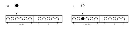
Figure 5. Two cases in an FC table. In a) $\bullet$ is the last key inserted, while in b) $\bullet$ is already in the table when the last key is inserted.

As a consequence we have the specification:

$$FC=\operatorname{Add}\bigl{(}\operatorname{Pos}_{q}(AF)*AF+\operatorname{Pos}(FC)*AF+\operatorname{Pos}(AF)*FC\bigr{)},$$ (12.7)

where $\operatorname{Pos}_{q}$ means that we operate on the generating functions by $\mathsf{H}$ in (5.3), while the normal $\operatorname{Pos}$ operates by $\frac{w}{b}\frac{\partial}{\partial w}$ as in Figure 2. The construction $\operatorname{Add}$ translates to integration $\int$, see Section 5; we eliminate this by taking the derivative $\partial/\partial z$ on both sides. The specification (12.7) thus yields the partial differential equation

$$\frac{\partial}{\partial z}FC(z,w,q)=\mathsf{H}[AF(z,w)]AF(z,w)\\ +w\frac{\partial}{\partial w}\bigl{(}FC(z,w,q)\bigr{)}~{}AF(z,w)+w\frac{\partial}{\partial w}\bigl{(}AF(z,w)\bigr{)}FC(z,w,q).$$ (12.8)

Moreover, since all generating functions here are for almost full tables, with $n=m-1$, they are all of the form $F(wz)/z$, and we have $z\partial_{z}=w\partial_{w}-1$. Thus, (12.8) reduces to the ordinary differential equation

$$\bigl{(}1-zAF(z,w)\bigr{)}w\frac{\partial}{\partial w}FC(z,w,q)=\Bigl{(}1+w\frac{\partial}{\partial w}\bigl{(}zAF(z,w)\bigr{)}\Bigr{)}FC(z,w,q)\\ +z\mathsf{H}[AF(z,w)]AF(z,w).$$ (12.9)

Furthermore, since $b=1$, (4.1) yields $AF(z,w)=wF_{0}(zw)=N_{0}(z,w)$, which by (4.2) or (4.6) yields $AF(w,z)=T(zw)/z$. Substituting this in (12.9), the differential equation is easily solved using (3.3) and the integrating factor $(1-T(zw))/T(zw)$, and we obtain the following theorem.

Theorem 12.2.

For $b=1$,

$$FC(z,w,q)=\frac{\bigl{(}(1-T(zwq))^{2}-(1-T(zw))^{2}\bigr{)}T(zw)}{2z(1-q)(1-T(zw))}.$$ (12.10)

Note that a similar derivation has been done in Section 4.6 of [38]. The difference is that in [38] a recurrence for $n![z^{n}w^{n+1}]$ is derived, and then moments are calculated. Even though it could have been done, no attempt to find the generating function from the recurrence is presented there. Moreover, in [39], the same recurrence as in [38] is presented and then the distribution is explicitly calculated for the Poisson model (although the distribution is not presented for the combinatorial model).

Here, with the same specification, the symbolic method leads directly to the generating function, avoiding the need to solve any recurrence. This example presents in a very simple way how to use the approach “if you can specify it, you can analyze it”.

By (12.6) and (4.8), we obtain immediately the generating function $FCFS$ (for general hash tables) in the case $b=1$.

Theorem 12.3.

For $b=1$,

$$FCFS(z,w,q)=\frac{((1-T(zwq))^{2}-(1-T(zw))^{2})T(zw)}{2(1-q)(1-T(zw))(z-T(zw))}.$$

The distribution of the displacement $D^{\mathsf{FC}}_{m,n}$ can be obtained by extracting coefficients in $FCFS$, see (12.1)–(12.2). Instead of doing this, we just quote a result from Theorem 5.1 in [39] (see also [21, Theorem 5.2]): If $b=1$, $1\leqslant n\leqslant m$ and $k\geqslant 0$, then

$$[q^{k}]d_{m,n}(q)=1-\frac{n-1}{2m}-\sum_{j=0}^{k-1}\binom{n-1}{j}\frac{(j+1)^{j-2}(m-j-1)^{n-j-1}}{m^{n-1}}.$$ (12.11)

Notice that there are two shifts from [39]: the first one in $k$ since in [39] the studied random variable is the search cost and here it is the displacement; the second one in $n$, since in [39] the table has $n+1$ elements.

We can also derive a formula similar to Theorem 12.2 for completely full tables. Let $FC_{0}(z,w,q)$ be the generating function for the displacement of a marked key $\bullet$ in a full table (with $n=m$ keys) such that the last key is inserted in the last bucket. (By rotational symmetry, we might instead require that any given key, or $\bullet$, is inserted in any given bucket, or that any given key, or $\bullet$, hashes to a given bucket.)

Theorem 12.4.

For $b=1$,

$$FC_{0}(z,w,q)=\frac{{(1-T(zwq))^{2}-(1-T(zw))^{2}}}{2(1-q)(1-T(zw))}.$$ (12.12)

Proof.

A full table is obtained by adding a key to an almost full table. This leads to the specification $FC_{0}=\operatorname{Add}(\operatorname{Pos}_{q}(AF)+\operatorname{Pos}(FC))$ and a differential equation that yields the result. However, we prefer instead the following combinatorial argument: Say that there is a cut-point after each bucket where the overflow is 0. By the rotational symmetry, we may equivalently define $FC_{0}$ as the class of full hash tables with a marked element $\bullet$ such that the first cut-point after $\bullet$ comes at the end of the table. By appending an almost full table to such a table, we obtain a table of the type $FC$; this yields a specification $FC=FC_{0}*AF$, since this operation is a bijcetion, with an inverse given by cutting a table of the type $FC$ at the first cut-point after $\bullet$. Consequently,

$$FC(z,w,q)=FC_{0}(z,w,q)AF(z,w)=FC_{0}(z,w,q)\frac{T(zw)}{z}$$ (12.13)

and the result follows by (12.10). ∎

Moments are easily obtained from the generating functions above. In particular, this gives another proof of (2.3)–(2.4):

Corollary 12.5.

For $b=1$,

$$\operatorname{\mathbb{E}{}}D^{\mathsf{FC}}_{n,n} =\frac{\sqrt{2\pi}}{4}n^{1/2}-\frac{2}{3}+\frac{\sqrt{2\pi}}{48n^{1/2}}-\frac{2}{135n}+O\bigl{(}n^{-3/2}\bigr{)},$$ (12.14)

$$\operatorname{Var}(D^{\mathsf{FC}}_{n,n}) =\frac{\sqrt{2\pi}}{12}n^{3/2}+\left(\frac{1}{9}-\frac{\pi}{8}\right)n+\frac{13\sqrt{2\pi}}{144}n^{1/2}-\frac{47}{405}-\frac{\pi}{48}+O\bigl{(}n^{-1/2}\bigr{)}.$$ (12.15)

Proof.

Taking $q=1$ in (12.12) we obtain (by l’Hôpital’s rule) $T(zw)/(1-T(zw))=(1-T(zw))^{-1}-1$, which is the EGF of $n^{n}$; this is correct since $FC_{0}$ counts the full tables with a marked key such that the last key is inserted in the last bucket, and there are indeed $n^{n}$ such tables.

Taking the first and second derivatives of (12.12) at $q=1$ we find, with $T=T(zw)$,

$$\sum_{n=1}^{\infty}n^{n}\operatorname{\mathbb{E}{}}D^{\mathsf{FC}}_{n,n}\frac{(zw)^{n}}{n!} =\mathsf{U}_{q}\partial_{q}FC_{0}(z,w,q)=\frac{T^{2}}{2(1-T)^{2}}$$

$$=\frac{1}{2(1-T)^{2}}-\frac{1}{1-T}+\frac{1}{2},$$

$$\sum_{n=1}^{\infty}n^{n}\operatorname{\mathbb{E}{}}(D^{\mathsf{FC}}_{n,n})^{2}\frac{(zw)^{n}}{n!} =\mathsf{U}_{q}\partial_{q}^{2}FC_{0}(z,w,q)+\mathsf{U}_{q}\partial_{q}FC_{0}(z,w,q)=\frac{3T^{2}-T^{4}}{6(1-T)^{4}}$$

$$=\frac{1}{3(1-T)^{4}}-\frac{1}{3(1-T)^{3}}-\frac{1}{2(1-T)^{2}}+\frac{2}{3(1-T)}-\frac{1}{6}.$$

Knuth and Pittel [27] defined the tree polynomials $t_{n}(y)$ as the coefficients in the expansion

$$\frac{1}{(1-T(z))^{y}}=\sum_{n=0}^{\infty}t_{n}(y)\frac{z^{n}}{n!}.$$ (12.16)

By identifying coefficients, we thus obtain the exact formulas

$$n^{n}\operatorname{\mathbb{E}{}}D^{\mathsf{FC}}_{n,n} =\tfrac{1}{2}t_{n}(2)-t_{n}(1),$$ (12.17)

$$n^{n}\operatorname{\mathbb{E}{}}(D^{\mathsf{FC}}_{n,n})^{2} =\tfrac{1}{3}t_{n}(4)-\tfrac{1}{3}t_{n}(3)-\tfrac{1}{2}t_{n}(2)+\tfrac{2}{3}t_{n}(1).$$ (12.18)

The result now follows from the asymptotic of $t_{n}(y)$ obtained by singularity analysis, see [27, (3.15) and the comments below it]. ∎

Remark 12.6.

The approach in this subsection can in principle be used also for $b>1$. For $1\leqslant k\leqslant b$, let $AF_{k}(z,w)$ be the generating function for almost full hash tables with $k$ empty slots in the last bucket, and let $FC_{k}(z,w,q)$ be the generating function for such tables with a marked key $\bullet$, with $q$ marking the displacement of $\bullet$. We can for each $k$ argue as for (12.7), but we now also have the possibility that the last key hashes to an almost full table with $k+1$ empty slots (provided $k<b$). We thus have the specifications

$$FC_{k}=\operatorname{Add}\bigl{(}\operatorname{Pos}_{q}(AF_{1})*AF_{k}+\operatorname{Pos}(FC_{1})*AF_{k}+\operatorname{Pos}(AF_{1})*FC_{k}\\ +\operatorname{Pos}_{q}(AF_{k+1})+\operatorname{Pos}(FC_{k+1})\bigr{)},\qquad k=1,\dots,b$$ (12.19)

with $AF_{b+1}=FC_{b+1}=\emptyset$. This yields a system of $b$ differential equations similar to (12.9) for the generating functions $FC_{k}(z,w,q)$; note that $AF_{k}$ is given by $F_{b-k}$ in (4.1) and (4.2). However, we do not know any explicit solution to this system, and we therefore do not consider it further, preferring the alternative approach presented in Section 12.1. (It seems possible that this approach at least might lead to explicit generating functions for the expectation and higher moments by differentiating the equations at $q=1$, but we have not pursued this.)

12.3. Probabilistic approach

In the probabilistic model, when inserting a new key in the hash table with the FCFS rule, we do exactly as in an unsuccessful search, except that at the end we insert the new key. Hence the displacement of a new key has the same distribution as $U_{i}$ in Section 11. However (unlike the RH rule), the keys are never moved once they are inserted, and when studying the displacement of a key already in the table, we have to consider $U_{i}$ at the time the key was added.

We consider again infinite hashing on $\mathbb{Z}$, and add a time dimension by letting the keys arrive to the buckets by independent Poisson process with intensity 1. At time $t\geqslant 0$, we thus have $X_{i}\sim\operatorname{Po}(t)$, so at time $\alpha b$ we have the same infinite Poisson model as before, but with each key given an arrival time, with the arrival times being i.i.d. and uniformly distributed on $[0,\alpha b]$. (We cannot proceed beyond time $t=b$; at this time the table becomes full and an infinite number of keys overflow to $+\infty$; however, we consider only $t<b$.)

Consider the table at time $\alpha b$, containing all key with arrival times in $[0,\alpha b]$. We are interested in the FCFS displacement of a “randomly chosen key”. Since there is an infinite number of keys, this is not well-defined, but we can interpret it as follows (which gives the correct limit of finite hash tables, see the theorem below): By a basic property of Poisson processes, if we condition on the existence of a key, $x$ say, that arrives to a given bucket $i$ at a given time $t$, then all other keys form a Poisson process with the same distribution as the original process. Hence the FCFS displacement of $x$ has the same distribution as $U_{\beta}$, computed with the load factor $\alpha$ replaced by $\beta:=t/b$. Furthermore, as said above, the arrival times of the keys are uniformly distributed in $[0,\alpha b]$, so $\beta$ is uniformly distributed in $[0,\alpha]$. Hence, the FCFS displacement $D^{\mathsf{FC}}=D^{\mathsf{FC}}_{\alpha}$ of a random key is (formally by definition) a random variable with the distribution

$$\Pr(D^{\mathsf{FC}}_{\alpha}=k)=\frac{1}{\alpha}\int_{0}^{\alpha}\Pr\bigl{(}U_{\beta}=k\bigr{)}\,\mathrm{d}\beta.$$ (12.20)

This leads to the following, where we now write $\alpha$ as an explicit parameter of all quantities that depend on it.

Theorem 12.7.

In the infinite Poisson model, the probability generating function $\psi_{\mathsf{FC}}(q;\alpha):=\operatorname{\mathbb{E}{}}q^{D^{\mathsf{FC}}}$ of $D^{\mathsf{FC}}=D^{\mathsf{FC}}_{\alpha}$ is given by

$$\begin{split}\psi_{\mathsf{FC}}(q;\alpha)&=\frac{1}{\alpha}\int_{0}^{\alpha}\psi_{U}(q;\beta)\,\mathrm{d}\beta=\frac{1}{\alpha}\int_{0}^{\alpha}\frac{T_{0}(b\beta)}{1-q}\prod_{\ell=0}^{b-1}\bigl{(}1-\zeta_{\ell}(q;\beta)\bigr{)}\,\mathrm{d}\beta\\ &=\frac{1}{\alpha}\int_{0}^{\alpha}\frac{b(1-\beta)\prod_{\ell=0}^{b-1}\bigl{(}1-\zeta_{\ell}(q;\beta)\bigr{)}}{(1-q)\prod_{\ell=1}^{b-1}(1-\zeta_{\ell}(1;\beta))}\,\mathrm{d}\beta.\end{split}$$ (12.21)

Moreover, for the exact model, as $m,n\to\infty$ with $n/bm\to\alpha$, $D^{\mathsf{FC}}_{m,n}\overset{\mathrm{d}}{\longrightarrow}D^{\mathsf{FC}}_{\alpha}$ with convergence of all moments; furthermore, for some $\delta>0$, the probability generating function converges to $\psi_{\mathsf{FC}}(q)$, uniformly for $|q|\leqslant 1+\delta$.

Proof.

The first equality in (12.21) follows by (12.20), and the second by Theorem 11.2.

For the exact model, we have by the discussion above, for any $k\geqslant 0$,

$$\Pr(D^{\mathsf{FC}}_{m,n}=k)=\frac{1}{n}\sum_{j=1}^{n}\Pr\bigl{(}U_{m,j-1}=k\bigr{)}=\int_{0}^{1}\Pr\bigl{(}U_{m,\lfloor nx\rfloor}=k\bigr{)}\,\mathrm{d}x.$$

For any $x>0$, $\lfloor nx\rfloor/bm\overset{\mathrm{d}}{\longrightarrow}x\alpha$, and thus $\Pr\bigl{(}U_{m,\lfloor nx\rfloor}=k\bigr{)}\to\Pr\bigl{(}U_{x\alpha}=k\bigr{)}$ by Theorem 11.2. Hence, by dominated convergence and the change of variables $\beta=x\alpha$,

$$\Pr(D^{\mathsf{FC}}_{m,n}=k)\to\int_{0}^{1}\Pr\bigl{(}U_{x\alpha}=k\bigr{)}\,\mathrm{d}x=\frac{1}{\alpha}\int_{0}^{\alpha}\Pr\bigl{(}U_{\beta}=k\bigr{)}\,\mathrm{d}\beta=\Pr(D^{\mathsf{FC}}_{\alpha}=k),$$

by (12.20). Hence $D^{\mathsf{FC}}_{m,n}\overset{\mathrm{d}}{\longrightarrow}D^{\mathsf{FC}}_{\alpha}$ as $m,n\to\infty$ with $n/bm\to\alpha$. Convergence of moments and probability generating function follows by Lemma 10.8 and the estimate $D^{\mathsf{FC}}\leqslant U_{i}\leqslant\hat{B}_{i}$ for a key that hashes to $i$. ∎

Corollary 12.8.

As $m,n\to\infty$ with $n/bm\to\alpha\in(0,1)$,

$$\operatorname{\mathbb{E}{}}D^{\mathsf{FC}}_{m,n} \to\operatorname{\mathbb{E}{}}D^{\mathsf{FC}}_{\alpha}=\operatorname{\mathbb{E}{}}D^{\mathsf{RH}}_{\alpha}=\frac{1}{2b\alpha}\biggl{(}\frac{1}{1-\alpha}-b-b\alpha\biggr{)}+\frac{1}{b\alpha}\sum_{\ell=1}^{b-1}\frac{1}{1-\zeta_{\ell}}.$$ (12.22)

Proof.

The convergence follows by Theorem 12.7. In the exact model, $\operatorname{\mathbb{E}{}}D^{\mathsf{FC}}_{m,n}=\operatorname{\mathbb{E}{}}D^{\mathsf{RH}}_{m,n}$, since the total displacement does not depend on the insertion rule, see Lemma 9.2. Hence, using also Corollary 9.4, $\operatorname{\mathbb{E}{}}D^{\mathsf{FC}}_{\alpha}=\operatorname{\mathbb{E}{}}D^{\mathsf{RH}}_{\alpha}$, and the result follows by (9.17). Alternatively, by (12.20),

$$\operatorname{\mathbb{E}{}}D^{\mathsf{FC}}_{\alpha}=\frac{1}{\alpha}\int_{0}^{\alpha}\operatorname{\mathbb{E}{}}U_{\beta}\,\mathrm{d}\beta,$$ (12.23)

where $\operatorname{\mathbb{E}{}}U_{\beta}$ is given by (11.6). It can be verified that this yields (12.22) (simplest by showing that $\frac{\mathrm{d}}{\mathrm{d}\alpha}\bigl{(}\alpha\operatorname{\mathbb{E}{}}D^{\mathsf{RH}}_{\alpha}\bigr{)}=\operatorname{\mathbb{E}{}}U_{\alpha}$, using (9.17), (3.5) and (3.3)). ∎

13. Some experimental results

In this section we check our theoretical results against the experimental values for the FCFS heuristic presented in the original paper [33] from 1957, where the linear probing hashing algorithm was first presented, since this is the first distributional analysis made for the problem (for the general case, $b\geq 1$).

The historical value of this section, relies on the fact that this is the first time that these original experimental values are checked against distributional theoretical results.

Length	# records	Length $\times$ #	Empirical prob.	Theoretical
1	8418	8418	0.9353	0.9352
2	336	672	0.0373	0.0364
3	111	333	0.0123	0.0122
4	70	280	0.0078	0.0059
5	26	130	0.0029	0.0033
6	9	54	0.0010	0.0020
7	14	98	0.0016	0.0013
8	7	56	0.0008	0.0009
9	5	45	0.0006	0.0006
10	1	10	0.0001	0.0005
11	1	11	0.0001	0.0003
12	0	0	0.0000	0.0003
13	1	13	0.0001	0.0002
14	1	14	0.0001	0.0002
sum$|$average	9000	10134	1.1260	1.1443

Figure 6. Table 3 in [33], with $b=20$, $m=10000$ and $n=9000$ ($\alpha=0.9$), together with theoretical results taken from our distributional results in the Poisson Model for the FCFS heuristic, Theorem 12.7. For the keys with low search cost (3 or less) there is a very good agreement with the experimental results. This is consistent with the explanation that the high variance is originated by all the latest keys inserted (and as a consequence, in FCFS, by the ones with larger displacement). The last line presents the average search cost, where a difference with the theoretical result in Corollary 12.8 is noticed.

Even though we have exact distributional results for the search cost of random keys by Theorem 12.1 for the generating function, the coefficients are very difficult to extract and to calculate. As a consequence, except for the case when $b=1$ where exact results are easy to use by means of (2.1), we use the asymptotic approximate results in the Poisson Model derived in Theorem 12.7 and Corollary 12.8. Notice that Theorem 12.7 and Corollary 12.8 evaluate the displacement of a random key, while in [33] its search cost is calculated. As a consequence, we have to add 1 to the theoretical results. When the table is full, we use (9.9).

% Full	1st run	2nd run	3rd run	4th run	Theoretical
40	1.000	1.000	1.000	1.000	1.000
60	1.001	1.002	1.002	1.003	1.002
70	1.008	1.013	1.009	1.010	1.010
80	1.026	1.043	1.029	1.035	1.036
85	1.064	1.073	1.062	1.067	1.069
90	1.134	1.126	1.138	1.137	1.144
95	1.321	1.284	1.331	1.392	1.386
97	1.623	1.477	1.512	1.797	1.716
99	2.944	2.112	2.085	2.857	3.379
100	4.735	3.319	3.830	4.299	4.002

Figure 7. Table 4 in [33]: average length of search of a random record with $b=20$ and $m=500$, together with theoretical results. (The experiments were carried four times over the same data.) As $\alpha$ increases, so does the variance of the results for the four runs.

All the simulations in [33] were done in random-access memory with a IBM 704 addressing asystem (simulated memory with random identification numbers). It is interesting to note that the IBM 704 was the first mass-produced computer with floating-point arithmetic hardware. It was introduced by IBM in 1954.

	$b=1~{}|~{}m=500$					$b=2~{}|~{}m=500$
% Full	Experimental	Poisson	Exact		% Full	Experimental	Poisson
10	1.053	1.056	1.055		20	1.034	1.024
20	1.137	1.125	1.125		40	1.113	1.103
30	1.230	1.214	1.213		60	1.325	1.293
40	1.366	1.333	1.331		70	1.517	1.494
50	1.541	1.500	1.496		80	1.927	1.903
60	1.823	1.750	1.741		90	3.148	3.147
70	2.260	2.167	2.142		95	5.112	5.644
80	3.223	3.000	2.911		100	11.389	10.466
90	5.526	5.500	4.889
100	16.914	—	14.848

Figure 8. Table 5B in [33]: average length of search with $b=1$ or 2 and $m=500$ (average of 9 runs over the same data), together with exact results taken from equation (2.1) and the Poisson approximation taken from Corollary 12.8 (and (9.9) for full tables). Notice that the Poisson approximation matches very well when the load factor is less than $0.9$. This is consistent with the fact that this approximation largely overestimates the exact result when $\alpha\to 1$.

The high variance of the FCFS heuristic is originated by the fact that the first keys stay in their home location, but when collisions start to appear, the search cost of the latest inserted keys increases very rapidly. For example, the last keys inserted have an $O(m)$ displacement in average. As an aside, for the case $b=1$ there are very interesting results that analyze the way contiguous clusters coalesce [9]. A good understanding of this process, leads to a rigurous explanation of this problem.

# Runs	8	7	4	4	3	3
% Full	b=5	b=10	b=20	b=30	b=40	b = 50
	bm=2500	bm=5000	bm=5000	bm=10000	bm=10000	bm=10000
40	1.015 (1.012)	1.001 (1.001)	1.000 (1.000)	1.000 (1.000)	1.000 (1.000)	1.000 (1.000)
60	1.072 (1.066)	1.016 (1.015)	1.002 (1.002)	1.001 (1.000)	1.000 (1.000)	1.000 (1.000)
70	1.131 (1.136)	1.042 (1.042)	1.010 (1.010)	1.003 (1.003)	1.001 (1.001)	1.000 (1.000)
80	1.280 (1.289)	1.111 (1.110)	1.033 (1.036)	1.017 (1.017)	1.011 (1.009)	1.005 (1.005)
85	1.443 (1.450)	1.172 (1.186)	1.066 (1.069)	1.038 (1.036)	1.028 (1.022)	1.015 (1.015)
90	1.762 (1.777)	1.330 (1.345)	1.134 (1.144)	1.082 (1.083)	1.071 (1.055)	1.034 (1.040)
95	2.467 (2.771)	1.755 (1.837)	1.334 (1.386)	1.231 (1.241)	1.185 (1.171)	1.110 (1.130)
97	3.154 (4.102)	2.187 (2.501)	1.602 (1.716)	1.374 (1.460)	1.399 (1.334)	1.228 (1.260)
99	4.950 (10.766)	3.212 (5.831)	2.499 (3.379)	1.852 (2.567)	2.007 (2.164)	1.585 (1.923)
100	6.870 (6.999)	4.889 (5.244)	4.041 (4.002)	2.718 (3.451)	2.844 (3.123)	2.102 (2.899)

Figure 9. Table 5A in [33]: average length of search. The first number is the experimental result, and in parenthesis the theoretical value. We see again that the disagreement is larger when $\alpha$ is close to 1.

As a consequence, as it is explicitly said in [33], the experiments had to be performed several times, and an average of the results are presented. Our theoretical results seem to agree well with the experimental values when the load factor is less than $\alpha=0.9$. Moreover, the closer the value of $\alpha$ gets to 1 then the larger the difference. This is expected, since the formulae are good approximations when $\alpha<1$, and tend to $\infty$ when $\alpha\to 1$.

Acknowledgements.

Philippe Flajolet has had a strong influence in our scientific careers. The core of the use of the symbolic method in hashing problems has been taken from [12]. Thank you Philippe for all the work you have left to inspire our research. We also thank Alois Panholzer for interesting discussions, and Hsien-Kuei Hwang for suggesting us the derivation that leads to Theorem 12.1.

References

• [1] O. Amble and D. E. Knuth, Ordered hash tables. Computer Journal, 17(2):135–142, 1974.
• [2] Patrick Billingsley, Convergence of Probability Measures. Wiley, New York, 1968.
• [3] Ian F. Blake and Alan G. Konheim, Big buckets are (are not) better! J. Assoc. Comput. Mach. 24(4):591–606, 1977
• [4] Richard P. Brent, Reducing the retrieval time of scatter storage techniques. C. ACM, 16(2):105–109, 1973.
• [5] Pedro Celis, Robin Hood Hashing. PhD thesis, Computer Science Department, University of Waterloo, April 1986. Technical Report CS-86-14.
• [6] Pedro Celis, Per-Åke Larson and J. Ian Munro, Robin Hood hashing. In 26th IEEE Sympusium on the Foundations of Computer Science, pages 281–288, 1985.
• [7] Philippe Chassaing and Philippe Flajolet, Hachage, arbres, chemins & graphes. Gazette des Mathématiciens 95:29–49, 2003.
• [8] Philippe Chassaing and Svante Janson, A Vervaat-like path transformation for the reflected Brownian bridge conditioned on its local time at 0. Ann. Probab. 29(4):1755–1779, 2001.
• [9] Philippe Chassaing and Guy Louchard, Phase transition for parking blocks, brownian excursion and coalescence. Random Structures & Algorithms, 21(1):76–119, 2002.
• [10] Ronald Fagin, Jurg Nievergelt, Nicholas Pippenger, and H. Raymond Strong, Extendible hashing - a fast access method for dynamic files. ACM Transactions on Database Systems, 4(3):315–344, 1979.
• Feller [1971] William Feller, An Introduction to Probability Theory and its Applications, Volume II. 2nd ed., Wiley, New York, 1971.
• [12] Philippe Flajolet, Slides of the lecture ”On the Analysis of Linear Probing Hashing”, 1998. http://algo.inria.fr/flajolet/Publications/lectures.html
• [13] Philippe Flajolet, Peter J. Grabner, Peter Kirschenhofer and Helmut Prodinger, On Ramanujan’s $Q$-function. Journal of Computational and Applied Mathematics 58:103–116, 1995.
• [14] Philippe Flajolet and Andrew M. Odlyzko, Singularity Analysis of Generating Functions. SIAM J. Discrete Math 3(2):216-240, 1990.
• [15] Philippe Flajolet, Patricio Poblete and Alfredo Viola, On the Analysis of Linear Probing Hashing. Algorithmica 22(4):490–515, 1998.
• [16] Philippe Flajolet and Robert Sedgewick, Analytic Combinatorics. Cambridge University Press, 2009.
• [17] Gaston H. Gonnet and Ricardo Baeza-Yates, Handbook of Algorithms and Data Structures: in Pascal and C. Addison–Wesley, second edition, 1991.
• [18] Gaston H. Gonnet and J. Ian Munro, Efficient ordering of hash tables. SIAM Journal on Computing, 8(3):463–478, 1979.
• [19] Allan Gut, Probability: A Graduate Course, 2nd ed., Springer, New York, 2013.
• [20] Svante Janson, Asymptotic distribution for the cost of linear probing hashing. Random Struct. Alg. 19(3-4):438–471, 2001.
• [21] Svante Janson, Individual displacements for linear probing hashing with different insertion policies. ACM Transactions on Algorithms, 1(2):177–213, 2005.
• [22] Svante Janson, Brownian excursion area, Wright’s constants in graph enumeration, and other Brownian areas. Probability Surveys 3:80–145, 2007.
• [23] Svante Janson, Tomasz Łuczak and Andrzej Ruciński, Random Graphs. Wiley, New York, 2000.
• [24] D. Knuth, Notes on “open” addressing. Unpublished memorandum, 1963. (Memo dated July 22, 1963. With annotation “My first analysis of an algorithm, originally done during Summer 1962 in Madison”. Also conjectures the asymptotics of the $Q$-function, with annotation “Proved May 24, 1965”.). Available at http://algo.inria.fr/AofA/Research/11-97.html
• [25] Donald E. Knuth, The Art of Computer Programming. Vol. 3: Sorting and Searching. 2nd ed., Addison-Wesley, Reading, Mass., 1998.
• [26] Donald E. Knuth, Linear Probing and Graphs. Algorithmica 22(4):561–568, 1998.
• [27] Donald E. Knuth and Boris Pittel, A recurrence related to trees. Proc. Amer. Math. Soc. 105(2):335–349, 1989.
• [28] Alan G. Konheim and Benjamin Weiss, An occupancy discipline and applications. SIAM Journal on Applied Mathematics, 6(14):1266–1274, 1966.
• [29] Per-Åke Larson, Analysis of uniform hashing. J. Assoc. Comput. Mach., 30(4):805–819, 1983.
• [30] Haim Mendelson, Analysis of linear probing with buckets. Information Systems, 8(3):207–216, 1983.
• [31] Frank W. J. Olver, Daniel W. Lozier, Ronald F. Boisvert and Charles W. Clark, NIST Handbook of Mathematical Functions. Cambridge Univ. Press, 2010.
Also available as NIST Digital Library of Mathematical Functions. http://dlmf.nist.gov/
• [32] Alois Panholzer, Slides of the lecture “Asymptotic results for the number of unsuccessful parkers in a one-way street”, 2009. http://info.tuwien.ac.at/panholzer/
• [33] W. W. Peterson, Addressing for random-access storage. IBM Journal of Research and Development 1(2):130–146, 1957.
• [34] Patricio V. Poblete and J. Ian Munro, Last-come-first-served hashing. Journal of Algorithms, 10:228–248, 1989.
• [35] Patricio V. Poblete, Alfredo Viola, and J. Ian Munro, The Diagonal Poisson Transform and its application to the analysis of a hashing scheme. Random Structures & Algorithms, 10(1-2):221–255, 1997.
• [36] Robert Sedgewick and Philippe Flajolet, An Introduction to the Analysis of Algorithms. Addison-Wesley, Reading, Mass., 1996.
• [37] Georg Seitz, Parking functions and generalizations. Diploma Thesis, TU Wien, 2009.
• [38] Alfredo Viola, Analysis of Hashing Algorithms and a New Mathematical Transform. PhD thesis, Computer Science Department, University of Waterloo, November 1995. Technical Report CS-95-50.
• [39] Alfredo Viola, Exact distribution of individual displacements in linear probing hashing. ACM Transactions on Algorithms, 1(2):214–242, 2005.
• [40] Alfredo Viola, Distributional analysis of the parking problem and Robin Hood linear probing hashing with buckets. Discrete Math. Theor. Comput. Sci. 12(2):307–332, 2010.
• [41] Alfredo Viola and Patricio V. Poblete, The analysis of linear probing hashing with buckets. Algorithmica, 21(1):37–71, 1998.