ANALYSIS OF LONG-RANGE STUDIES IN THE LHC – COMPARISON WITH THE MODEL

Abstract

We find that the observed dependencies (scaling) of long-range beam–beam effects on the beam separation and intensity are consistent with the simple assumption that, all other parameters being the same, the quantity preserved during different set-ups is the first-order smear as a function of amplitude.

1 Introduction

1.1 The Proposed Method

In several Machine Development (MD) studies (see Ref. [1] and the references therein), reduced crossing angles have been used to enhance long-range beam–beam effects and thus facilitate their measurement. The basic assumption made in this paper is that under such conditions, a single non-linearity, the one caused by beam–beam, dominates the dynamics. Hence the method followed: we choose some simple low-order dynamical quantity that characterizes phase space distortion and assume that when this quantity is the same, the behaviour of the system is the same. A most obvious candidate is the first-order smear – the r.m.s. deviation of the phase-space ellipse from the perfect one. At a fixed amplitude, smear is defined as the averaged generalized Courant–Snyder invariant over the angle variable [2].

An analytical expression has previously been found [2] for the smear $S$ as a function of amplitude $n_{\sigma}$. Suppose that the parametric dependence of $S(n)$ on several beam–beam related parameters – the relativistic $\gamma$, the number of particles per bunch $N_{b}$, the crossing angle $\alpha$, and the normalized separations $n_{\rm l.r.}$ – is known. According to the above assumption, for two machine configurations a and b one should have

$$S(n_{\sigma};N_{b}^{a},n^{a}_{\rm l.r.},\alpha^{a},\gamma^{a})=S(n_{\sigma};N_{b}^{b},n^{b}_{\rm l.r.},\alpha^{b},\gamma^{b}).$$ (1)

As a particular application of Eq. (1), we considered two experiments where the intensities are $N_{b}^{a}$ and $N_{b}^{b}$. All other parameters being the same, given $\alpha^{a}$, one can compute the expected $\alpha^{b}$. Our task will be to show that the result agrees with observations.

1.2 Analytical Calculation of Invariant and Smear

Our derivation of $S(n_{\sigma})$ is based on the Lie algebraic method – concatenation of Lie-factor maps – and is valid only to first order in the beam–beam parameter and in one-dimension, in either the horizontal or the vertical plane, but for an arbitrary distribution of beam–beam collisions, head-on or long-range, around the ring.

For a ring with a single head-on collision point, Hamiltonian perturbation analysis of the beam–beam interaction without or with a crossing angle has been done by a number of authors, mostly in the resonant case. Non-linear invariants of motion, both non-resonant and resonant, were analysed by Dragt [3], with the one-turn map as observed immediately after the kick being

$$R\;\mathrm{e}^{:{\mathit{F}}:}=\mathrm{e}^{:h:}\,.$$ (2)

Here, $R=\mathrm{e}^{:f_{2}:}$ is the linear one-turn map and the kick factor $F$ is the beam–beam potential (or Hamiltonian). For small perturbations and far from resonances, particle coordinates in phase space are restricted on the Poincaré surface of section

$$h=\mathrm{const}.$$ (3)

A detailed derivation of $h$ to first order in the beam–beam perturbation strength can be found in A. Chao’s lectures:

$$h(J,\phi)=-\mu J+\sum_{n=-\infty}^{\infty}{c^{\rm(ho)}_{n}(J)\frac{n\,\mu}{2\sin\frac{n\mu}{2}}\mathrm{e}^{in(\phi+\mu/2)}}\,,$$ (4)

where $\mu$ is the ring phase advance and $c^{\rm(ho)}_{n}(J)$ are coefficients in the Fourier expansion of $F$, when the latter is rewritten in action-angle coordinates $J,\phi$. The coefficients are shown to be related to the modified Bessel functions. Analytical expressions for the invariant $h$, the first-order smear, and the second-order detuning for the case of non-linear multipole kicks distributed in an arbitrary way around the ring have been derived by Irvin and Bengtsson [4]. Smear, the distortion of the ideal phase-space ellipse, is formally defined in Ref. [5]. Finally, note that extracting the smear is a natural step in the procedure that brings the map into its normal form [6].

In Ref. [7], following the Lie algebraic procedure in Refs. [8] and [4], we generalized Eq. (4) to describe multiple head-on kicks (IP1 and IP5) for the case of the LHC. In Ref. [2], an expression was presented that was valid for an arbitrary number of head-on (h.o.) and long-range (l.r.) collisions. This expression, to be derived in detail next, has been used on several occasions to interpret results from SixTrack simulations.

2 Derivation of the Invariant

2.1 Multiple Collision Points

The horizontal betatronic motion of a weak-beam test particle depends on its initial amplitude $n_{\sigma}$ (in units of $\sigma$) and the collision set: a set of all h. o. and l. r. collisions, also known as Interaction Points (IPs), that this particle sees over a single revolution. Let us label the set with an index $k$, limiting ourselves to only IPs located within the main interaction regions IR5 (horizontal crossing) and IR1 (vertical crossing). In the case of 50 ns bunch spacing, $k$ ranges from 1 to 34, which includes 32 long-range IPs ($N_{\rm l.\,r.~{}}=32$).

The Lie map depends on the above-defined collision set through the normalized separations $n^{(k)}_{x,y}=d^{(k)}_{x,y}/\sigma^{(k)}$ and the unperturbed horizontal betatronic phases $\phi^{(k)}$ at the IPs. Here, $d_{x,y}$ is the real-space offset of the strong-beam centroid in the $x$ or $y$ direction, and it has been assumed that both the weak- and strong-beam transverse distributions are round Gaussians of the same r.m.s. That is:

$$\sigma^{(k)}=\sqrt{\beta^{(k)}\epsilon}\ \ \ \ (\beta^{(k)}_{x}=\beta^{(k)}_{y}\equiv\beta^{(k)}).$$ (5)

In Eq. (5), $\beta^{(k)}$ are the beta functions and $\epsilon$ is the emittance. It will be shown below that off-plane collisions contribute very little to smear; thus after excluding these, the problem becomes one-dimensional and may easily be illustrated (see Fig. 1). Here, $n^{(k)}_{x}$ are the strong-beam centroids in amplitude space: points $(s^{(k)},n_{x}^{(k)})$, with $s$ being the distance to IP5 in metres.

Figure 1: A schematic view of weak- and strong-beam trajectories in real (top) and amplitude (bottom) spaces. A reduced set is used: $N_{\rm l.\,r.~{}}=8+8=16$ ($k=1,18$).

2.2 The Beam–Beam Hamiltonian

For a single collision (see Eq. (2)), by omitting the superscript $k$ in $\sigma$ and $n_{x,y}$, the $x$-motion is described by a kick factor $F$ (or Hamiltonian $H$) [2]:

$$F=-H(x) = \int_{0}^{P}(1-\mathrm{e}^{-\alpha})\frac{\mathrm{d}\alpha}{\alpha}\,=$$ (6)

$$= \overline{\gamma}+\Gamma_{0}(P)+\mathrm{ln}(P)\,,$$ (7)

$$P=P(x)=\frac{1}{2}\,\left[(n_{x}+\frac{x}{\sigma})^{2}+n_{y}^{2}\right]\,,$$

where $F$ is in units of $\lambda\equiv\frac{N_{b}r_{0}}{\gamma}$, $r_{0}$ is the classical particle radius, $\Gamma_{s}(P)\equiv\Gamma(s,P)$ denotes the upper incomplete gamma function [9], and $\overline{\gamma}$ = 0.577216 is Euler’s constant. The corresponding beam–beam kick is as follows:

$$\Delta x^{\prime}\equiv\frac{\mathrm{d}}{\mathrm{d}x}F(x)=\frac{\partial F}{\partial P}\frac{\mathrm{d}P}{\mathrm{d}x}=$$

$$= \frac{2(x+n_{x}\sigma)}{(x+n_{x}\sigma)^{2}+(n_{y}\sigma)^{2}}\left[1-\mathrm{e}^{-\frac{(x+n_{x}\sigma)^{2}+(n_{y}\sigma)^{2}}{2\sigma^{2}}}\right].$$ (8)

The Fourier expansion of $H$ is as follows:

$$H(n_{\sigma},\phi)=\sum_{m}{\cal C}_{m}\mathrm{e}^{im\phi}\,,$$ (9)

where ${\cal C}_{m}\equiv\frac{1}{2\pi}\int_{0}^{2\pi}\mathrm{e}^{-im\phi}H\;\mathrm{d}\phi$. These coefficients are easily computed numerically by using the implementation of $\Gamma$ in Mathematica [2]. Further, analytical expressions in the form of single integrals over Bessel functions have been derived in Ref. [10]. We display these again in the simplified case $n_{y}=0$ (no off-plane collisions):

$$\left.{\cal C}_{m}\right|_{n_{y}=0}=\displaystyle\int_{0}^{1}\frac{\mathrm{d}t}{t}\times$$

$$\begin{cases}\displaystyle[1-\mathrm{e}^{-\frac{t}{2}n_{x}^{2}}\mathrm{e}^{-\frac{t}{4}n_{\sigma}^{2}}\sum_{k=-\infty}^{\infty}I_{-2k}(t\,n_{\sigma}n_{x})I_{k}(-\frac{t}{4}n_{\sigma}^{2})]&\\ \mbox{if }m=0\mbox{ \ \ and}\\ \displaystyle-\mathrm{e}^{-\frac{t}{2}n_{x}^{2}}\mathrm{e}^{-\frac{t}{4}n_{\sigma}^{2}}\sum_{k=-\infty}^{\infty}i^{m}I_{m-2k}(t\,n_{\sigma}n_{x})I_{k}(-\frac{t}{4}n_{\sigma}^{2})&\\ \mbox{if }m\neq 0.\end{cases}$$

In the head-on case ($n_{x}^{(k)}=n_{y}^{(k)}=0$), the coefficients ${\cal C}_{m}$ reduce to the $c^{\rm(ho)}_{m}$ from Ref. [8]. Note that in the most interesting case, amplitudes near the dynamic aperture, both $n_{\sigma}$ and $n_{x}$ and hence the Bessel function arguments are large ($\gg 1$).

Our first step is to remove the linear and quadratic parts $F_{(1)}=\left.\frac{\partial F}{\partial x}\right|_{x=0}x$ and $F_{(2)}=\frac{1}{2}\left.\frac{\partial^{2}F}{\partial x^{2}}\right|_{x=0}\,x^{2}$. The non-linear kick factor and the corresponding kick are as follows:

$$F_{\rm nonl}=F-F_{(1)}-F_{(2)}\,\,,$$ (10)

$$\Delta x^{\prime}_{\rm nonl}\equiv\frac{d}{dx}F_{\rm nonl}(x)\,.$$

As a next step, we rewrite Eq. (10) in action-angle coordinates $J,\phi$ by substituting in it $x=\sqrt{2J\beta}\sin{\phi}=n_{\sigma}\sigma\sin{\phi}$, where $n_{\sigma}=\sqrt{2I}=\sqrt{2J/\epsilon}$ is the test particle amplitude (Eq. (A.1)). Next, we expand in Fourier series:

$$\displaystyle F_{\rm nonl}(n_{\sigma}\,\sigma\,\sin\phi)=c_{0}+\sum_{m\neq 0}c_{m}\mathrm{e}^{im\phi}\,.$$ (11)

The coefficients $c_{m}$ are naturally the same as ${\cal C}_{m}$ above, with the exception of $c_{1}$ and $c_{2}$, which contain additional $\mathrm{sin}$ and $\mathrm{sin}^{2}$ terms (see Eq. (A.1)).

2.3 Lie Map and Invariant

For an arbitrary set of collisions $n_{x}^{(k)}$, $\phi^{(k)}$ ($k=1,N$), we represent the LHC lattice by a combination of linear elements and non-linear kicks. It is shown in the Appendix that, to first order in $\lambda$, the Lie map has the same form as the one for a single kick (2) – where, however, the factor $F$ is given by the sum

$$F\equiv\sum_{k=1}^{{N}}F_{\rm nonl}^{(k)}(n_{\sigma},\phi)$$

and $F_{\rm nonl}^{(k)}$ are such that, compared to Eq. (11), the $k$th IP participates with a phase shifted by $\phi^{(k)}$:

$$F_{\rm nonl}^{(k)}(n_{\sigma},\phi)\equiv\left.F_{\rm nonl}^{(k)}(x)\right|_{x\;\rightarrow n_{\sigma}\,\sigma^{(k)}\,sin{(\phi+\phi^{(k)})}}=$$

$$=\sum_{m\neq 0}C_{m}^{(k)}\mathrm{e}^{im\phi}\,.$$ (12)

The shift in phase means that the coefficients in Eq. (12) are simply related to $c_{m}^{(k)}$: $C_{m}^{(k)}\equiv c_{m}^{(k)}\mathrm{e}^{im\phi^{(k)}}$ and still satisfy $C_{-m}=C_{m}^{\star}$. Another important property of the expansion is that only the oscillating part is taken (the $m=0$ term is excluded). The invariant for multiple collision points is as follows (see the Appendix):

$$h(I,\phi)=-\mu J-\lambda\displaystyle\sum_{k=1}^{N}\sum_{m=1}^{\infty}\frac{m\,\mu\,{c}^{(k)}_{m}(I)}{2\sin{(\frac{m\mu}{2})}}\mathrm{e}^{im(\phi+\mu/2+\phi^{(k)})}$$

$$+\;c.c.$$

The surface of the section in phase space is given by $h(I,\phi)=\mathrm{const}$. A natural initial condition is now imposed: that the initial point in phase space for a particle starting at $x_{0}=n_{\sigma}\sigma$ – that is, with an amplitude $I_{0}\equiv J_{0}/\epsilon=n_{\sigma}^{2}/2$ – lies on the curve representing the invariant:

$$h(I,\phi)=h(I_{0},\pi/2),$$ (13)

For a fixed $I_{0}$, this equation implicitly defines $I$ as a function of $\phi$. It satisfies the initial condition $I(0)=I_{0}$:

$$\displaystyle I(\phi)=I_{0}+\sum_{k=1}^{{N}}\left(\mathrm{d}I^{(k)}(\phi)-\mathrm{d}I^{(k)}(0)\right)\,,$$

$$\mathrm{d}I^{(k)}(\phi)=$$ (14)

$$=\displaystyle\frac{\lambda}{\epsilon}\sum_{m=1}^{M}\left(\frac{m\,{c}^{(k)}_{m}(I_{0})}{2\sin{(m\mu/2)}}\mathrm{e}^{im(\mu/2+\phi-\phi^{(k)}+\pi/2)}+c.c.\right).$$

Note that, to first order, the argument in ${c}^{(k)}_{m}$ has been replaced with $I_{0}$. We have also separated the two sums so that $\mathrm{d}I^{(k)}(\phi)-\mathrm{d}I^{(k)}(0)$ is the individual contribution of the $k$th IP. In the same way, a different initial condition may be used (more suitable for plots): $I(0)=I_{0}$, instead of $I(\pi/2)=I_{0}$.

The smear $S(n_{\sigma})$ is now defined as the normalized r.m.s. of the invariant – that is, $\sqrt{V}$, with $V$ being the variance:

$$S(n_{\sigma})={\sqrt{V}}/{\langle\,I\,\rangle}\,,$$

$$V=\frac{1}{2\pi}\int(I-\langle I\rangle)^{2}\mathrm{d}\phi\,,\ \ \ \ \langle I\rangle=\frac{1}{2\pi}\int I\mathrm{d}\phi\,.$$

3 Verification with tracking

As an example application, this section studies the very simple collision set that still possesses all the symmetries with the l.r. set at 8 sigma, as depicted in Fig. 2. Both IR5 and IR1 are included. The goal here is to test the invariant $I(\phi)$ by tracking with a simple model built with kicks $\Delta x^{\prime}_{\rm nonl}$ alternating with linear matrices and SixTrack. The parameters are as follows: energy $3.5~{}$TeV, $N_{\rm b}=1.2\times 10^{11}$, and normalized emittance $\epsilon_{n}=2.5\times 10^{-6}$.

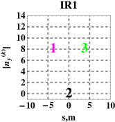
Figure 2: The sample set-up: three collisions in each IR5 and IR1. The l.r. are set at 8 sigma.

Tracking single particles at various amplitudes with the simple model produces the results shown in Fig. 3. A particle starts with $n_{\sigma}=3$, or $7$ ($I_{0}=4.5$, or $24.5$). The $c_{m}$ are computed with an accuracy of $10^{-7}$ – the value of $M$ in Eq. (2.3) is about $40$.

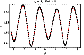
Figure 3: An invariant tested on a simple kick-matrix model. Black points: turn-by-turn coordinates ($\phi,I$) for $10^{3}$ turns. Red: invariant $I(\phi)$ (initials chosen so that $I(\pi/2)=I_{0}$).

Since the beam–beam potential changes the linear optics, we need to find the linearly perturbed matched $\beta$-function value at the initial point for tracking. For the plots in Fig. 3, this is done in a separate run, using a linear kick $(\Delta x^{\prime})_{\rm lin}$ (only terms $\sim x^{2}$ in the Hamiltonian). This is similar to what is done in SixTrack. The resultant matched $\beta$ is used to define the initial coordinate $x_{0}$ (through $n_{\sigma}$). The values of the smear are shown at the top of each plot.

Plotting the smear over a range of amplitudes with all three methods – model, SixTrack, and analytical $S(n_{\sigma})$ – results in Fig. 4. Note that here the images of the strong-beam centroids (see Fig. 1) are represented by vertical grey lines drawn at $0$ and $8$ sigma.

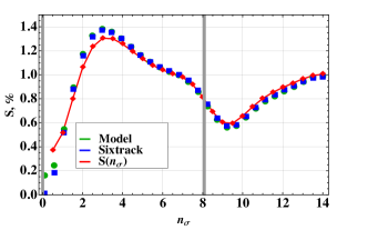
Figure 4: Agreement with SixTrack.

Let us now look at the individual contributions to $I(\phi)$ of the six IPs at three amplitudes chosen arbitrarily; say, $n_{\sigma}=1,3$, and $7$.

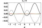
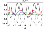
Figure 5: Individual contributions $dI^{(k)}(\phi)-dI^{(k)}(0)$ – color code as in Fig. 2.

The excursions (w.r.t. $I_{0}$) of the individual invariant surfaces are shown in Fig. 5. Here, $I(0)=I_{0}$. The colour code is as in Fig. 2, and in addition for the head-ons we use solid black for IP5 and dashed for IP1. Near the axis ($n_{\sigma}=1$), only the two head-ons contribute and, being of opposite signs, almost compensate each other. At $n_{\sigma}=3$, one begins to see long-range contributions that grow when $n_{\sigma}=7$. At such large amplitudes, the compensation is no longer true. Magenta and green are barely seen, meaning that the contribution of off-plane collisions is negligible. Thus in the case of a test particle moving in the horizontal motion, the contribution of all l.r. in IR1 can be neglected, and vice versa for vertical motion and IP5.

4 The behaviour of the smear $S(n_{\sigma})$ near the dynamic aperture

Above some critical strength of beam–beam interaction – that is, quantities $N_{\rm l.\,r.~{}}$ and/or $N_{\rm b}$ and/or an inverse crossing angle – the first-order theory is no longer an adequate description of the smear. However, as we will see, the behaviour of $S(n_{\sigma})$ may still be used as an indication of the dynamic aperture, since it exhibits a local maximum near it.

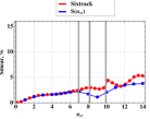
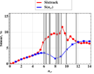
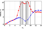
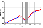
Figure 6: Various combinations of numbers of long-range collisions and bunch intensities to illustrate linear and non-linear behaviour:

	$N_{\rm l.\,r.~{}}$	$N_{\rm b}$
(a)	$16$	$1.2\times 10^{11}$
(b)	$32$	$1.2\times 10^{11}$
(c)	$32$	$1.6\times 10^{11}$
(d)	$32$	$0.2\times 10^{11}$

What happens is that the linear behaviour – that is, the agreement between the first-order $S$ and SixTrack at all amplitudes seen in Fig. 4 – is replaced by what is shown in Figs.  6(a)–(c). The blue ($S(n_{\sigma})$) and the red (SixTrack) curves depart from each other once $n_{\sigma}$ approaches amplitudes near the strong-beam core, represented by the cluster of vertical grey lines. At this point, the exact smear (red) exhibits a steep growth; thus the dynamic aperture is likely to be close to this point, while $S$ goes through a maximum and then through a minimum, thus forming a dip. Upon exiting the core, past the last grey line, the red and blue curves almost re-merge. It can be shown that the above property of $S(n_{\sigma})$ is a consequence of the left–right symmetry of IR5 and IR1. Namely, the individual contributions (such as the red and blue curves in Fig. 2) change sign or flip about the axis each time $n_{\sigma}$ crosses a grey line. At this amplitude, $S(n_{\sigma})$ stops growing and goes through a maximum.

5 Analysis of long-range experiments

5.1 Dependence on Intensity and Crossing Angle

We set the parameters as at the MD: energy $3.5~{}$TeV, $\epsilon_{n}=2.5\times 10^{-6}$ [11], and $\beta^{\star}=0.6$ m.

Of all the collision sets used at the MD, let us consider three: $N_{\rm l.\,r.~{}}=32$, 24, and 16. For each of them, two parameters, the bunch intensity $N_{\rm b}$ and the (half) crossing angle $\alpha$, uniquely define the dependence of the first-order smear on amplitude $S(n_{\sigma};N_{\rm b},\alpha)$ through the following procedure. First, being a first-order quantity in $\lambda$, the smear is obviously proportional to the intensity: $S\sim N_{\rm b}$. Second, the dependence of $n_{x,y}^{(k)}$ on the (half) crossing angle $\alpha$ is given by the well-known scaling law: $n_{x,y}^{(k)}\sim\alpha\sqrt{\beta^{\star}}$, where $n_{x,y}^{(k)}$ are taken from some sample lattice built for $\beta^{\star}=0.55$ m and $\alpha=125$. Finally, the phases $\phi^{(k)}$ are assumed to be independent of $\alpha$.

The dependence on the angle is presented in Fig. 7. Each blue branch corresponds to $S(n_{\sigma};1.2\times 10^{11},\alpha)$ being taken over an amplitude range where it is monotonically increasing; hence, as we already know, it will remain in agreement with the tracking for any strength of the beam–beam interaction.

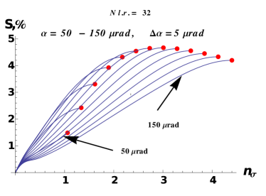
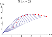
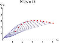
Figure 7: The dependence of the smear(amplitude) graph on the parameter $\alpha$ for $N_{\rm l.\,r.~{}}=32$ (top) and $N_{\rm l.\,r.~{}}=24$, $16$ (bottom). Each graph is restricted within a domain extending up to its first maximum (red dot) (the entrance into the strong-beam core).

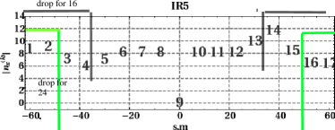
Figure 8: The collision sets for $N_{\rm l.\,r.~{}}$=24 and 16 are built by dropping the first and last two or four elements from the full set ($N_{\rm l.\,r.~{}}=32$).

Coming now to the MD, the observed losses during reduction of the crossing angle in IP1 are shown in Figs. 10 and 10 [1].

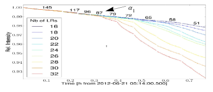
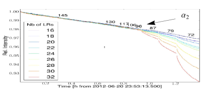
Figure 9: An experiment with $N_{\rm b}=1.2\times 10^{11}$: losses start at $\alpha_{1}\approx 87\;~{}\mu{\rm rad}$.

Figure 10: An experiment with $N_{\rm b}=1.6\times 10^{11}$: losses start at $\alpha_{1}\approx 96~{}\mu{\rm rad}$.

5.2 An Explanation of the Case $N_{\rm l.\,r.~{}}=32$ (Brown Curves)

For $N_{\rm l.\,r.~{}}=32$ (the full $50$-ns collision set shown in Fig. 8), we need to explain the brown curves in Figs. 10 and 10. Here, losses are seen to start at $\alpha_{1}\approx 87$ and $\alpha_{2}\approx 96~{}\mu{\rm rad}$, respectively.

In view of our previous findings, the off-plane losses (in IR5) are neglected and by using the postulate made in the Introduction (Eq. 1), we have:

$$S(n_{\sigma};1.2\times 10^{11},\alpha_{1})=S(n_{\sigma};1.6\times 10^{11},\alpha_{2}),$$ (15)

which is to be solved for the angles.

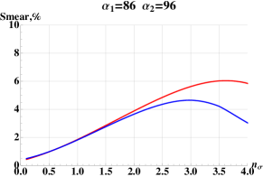
Figure 11: Graphs of $S(n_{\sigma};1.2\times 10^{11},86)$ (red) and $S(n_{\sigma};1.6\times 10^{11},96)$ (blue). The smear is seen to be $\approx 3\%$ at 1.5 $\sigma$.

Figure 11 shows that a good solution to Eq. (15) consists of the values $\alpha_{1}=86$, $\alpha_{2}=96~{}\mu{\rm rad}$. Indeed, this figure shows that Eq. (15) is fulfilled not in a single point, but for all amplitudes up to 1.5 $\sigma$, where the smear reaches $\approx 3\%$. What has happened, of course, is that scaling by a factor $1.6/1.2$, but reducing the angle from $\alpha_{2}$ to $\alpha_{1}$, has almost exactly preserved one particular blue branch from Fig. 7. Conversely, small variations about this solution, say $\pm 5~{}~{}\mu{\rm rad}$, lead to deviations of red and blue curves, as shown in Fig. 12.

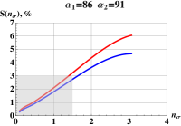
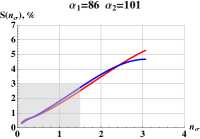
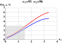
Figure 12: Small variations about the solution $\pm 5~{}~{}\mu{\rm rad}$.

5.3 Explanation of Cases $N_{\rm l.\,r.~{}}$=24 and 16 (Green and Black)

For $N_{\rm l.\,r.~{}}$=24 and 16 (reduced collision sets in Fig. 8), one needs to explain the green and black decay curves in Figs. 10 and 10. By looking now at the bottom two plots in Fig. 7, we search for blue branches that pass through the same maximum-smear point as found above: $3\%$ at 1.5 $\sigma$. The resultant branches are plotted in Figs. 13 and 14, with solution angles as summarized in Table 1. Again, at least a qualitative agreement is observed to the extent allowed by the resolution of Figs. 10 and 10.

Table 1: Angles of solutions for different intensities.

$N_{\rm b}$	Green	Black
$1.2\times 10^{11}$	65	53
$1.6\times 10^{11}$	83	72

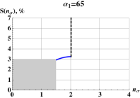
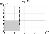
Figure 13: $N_{\rm b}=1.2\times 10^{11}$.

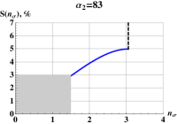
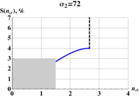
Figure 14: $N_{\rm b}=1.6\times 10^{11}$.

Of the four plots in Figs. 13 and 14, on three occasions the 3%-smear line intersects a monotonic part of $S(n_{\sigma})$ where, as we already know from Section 4, there is an exact agreement with SixTrack. The rough indication for the dynamic aperture, as the amplitude corresponding to a maximum of $S$, has been used in only one case: $\alpha$=53.

6 Appendix

The non-linear kick factor in Eq. (10) is

$$F_{\rm nonl}(n_{\sigma},\phi)=\gamma+\Gamma_{0}(P)+\mathrm{ln}(P)-F_{(1)}-F_{(2)}\,,$$

$$P=\frac{1}{2}\left((n_{x}+n_{\sigma}\sin{\phi})^{2}+n_{y}^{2}\right)\,,$$

$$F_{(1)}=\frac{2n_{x}}{(n_{x}^{2}+n_{y}^{2})}\left(1-\mathrm{e}^{-\frac{n_{x}^{2}+n_{y}^{2}}{2}}\right)n_{\sigma}\sin{\phi}\,,$$

$$F_{(2)}=\frac{-n_{x}^{2}+n_{y}^{2}+\mathrm{e}^{-\frac{n_{x}^{2}}{2}-\frac{n_{y}^{2}}{2}}\left(n_{x}^{2}+n_{x}^{4}-n_{y}^{2}+n_{x}^{2}n_{y}^{2}\right)}{\left(n_{x}^{2}+n_{y}^{2}\right)^{2}}\times$$

$$\times\,n_{\sigma}^{2}\sin^{2}\phi.\,\ \ \ \ \ \ \ \ \ \ \ \ \ \ \ \ \ \ \ \ \ \ \ \ \ \ \ \ \ \ {\rm(A.1)}$$

By following Ref. [4], the Lie map is given by an expression of the following form:

$$M_{N+1}\mathrm{e}^{:f^{(N)}:}M_{N}\dots\mathrm{e}^{:f^{(2)}:}M_{2}\mathrm{e}^{:f^{(1)}:}M_{1}\,,$$

$$f^{(k)}(x)\equiv F_{\rm nonl}^{(k)}(x).$$

Here, $M_{k}$ are linear operators and for brevity we have replaced $F_{\rm nonl}^{(k)}(x)$ with $f^{(k)}(x)$ . We will show that since $F_{\rm nonl}$ depends only on the normalized coordinate $x/\sigma$, once we rewrite it in terms of the eigen-coordinates at the $k$th kick, the local beta functions $\beta^{(k)}$ disappear, while the phase $\phi^{(k)}$ is simply added to $\phi$.

By reversing the order, the map transforming the test particle $(x,p_{x})$ for one turn around the ring is

$${\cal M}=M_{1}\mathrm{e}^{:f^{(1)}:}M_{2}\mathrm{e}^{:f^{(2)}:}\dots M_{N}\mathrm{e}^{:f^{(N)}:}M_{N+1}=$$

$$=\mathrm{e}^{:\overline{M}_{1}f^{(1)}:}\mathrm{e}^{:\overline{M}_{2}f^{(2)}:}\dots\mathrm{e}^{:\overline{M}_{N}f^{(N)}:}\overline{M}_{N+1}.$$

Reversal of the order means that in the first line all $f^{(k)}$ are now functions of the same initial variables $(x,p_{x})$. In the second line, accumulated linear maps $\overline{M}_{k}=M_{1}M_{2}...M_{k}$ have been applied to transform the initial vector to the kick location. Thus, as a first step, we have moved all kicks to the front of the lattice and $\overline{M}_{N+1}$ is the total one-turn linear Lie operator.

Let us denote matrices corresponding to Lie operators with hats; for example, $\widehat{M}_{N+1}$. As a second step, with $\beta$, $\alpha$ being matched Twiss parameters at the end of the lattice, one uses an $A_{0}$ transform that transforms the ring matrix to a rotation (inserting identities ${\cal A}_{0}{\cal A}^{-1}_{0}$ in between the exponents):

$$\widehat{M}_{N+1}\stackrel{{\scriptstyle{\widehat{\cal A}_{0}}}}{{\longrightarrow}}{\footnotesize\widehat{R}=\left(\begin{array}[]{cc}\cos\mu&\sin\mu\\ -\sin\mu&\cos\mu\end{array}\right)},$$

$${\widehat{\cal A}_{0}}=\left(\begin{array}[]{cc}\sqrt{\beta}&0\\ -\alpha/\sqrt{\beta}&1/\sqrt{\beta}\end{array}\right).$$

The two steps above combined are equivalent to replacing the argument of $f$ by $\widetilde{x}_{k}$ – the eigen-coordinate at the $k$th location. To see this, apply the ${\cal A}_{0}$ transform to both kick factor and coordinate:

$${\cal A}_{0}\overline{M}_{k}f^{(k)}(x)=f^{(k)}({\cal A}_{0}\overline{M}_{k}x)=f^{(k)}(\widetilde{x}_{k})\,,$$

$${\widetilde{x}_{k}}\equiv{\cal A}_{0}\overline{M}_{k}x=\sqrt{2\beta^{(k)}J}\sin{(\phi+\phi^{(k)})}\;.$$

One can now drop the ${\cal A}_{0}$ on both sides of $\cal M$ and consider the map:

$${\cal M}=\mathrm{e}^{:\widetilde{f}^{(1)}:}\mathrm{e}^{:\widetilde{f}^{(2)}:}\dots\mathrm{e}^{:\widetilde{f}^{({N})}:}R,$$

$$\widetilde{f}^{(k)}(J,\phi)=f^{(k)}(\widetilde{x}_{k}),$$

$$R=\mathrm{e}^{:f_{2}:},\ \ \ \ \ \ \ {:f_{2}:}=-\mu J.$$

To first order, one can just sum the Lie factors:

$${\cal M}\approx\mathrm{e}^{:F:}\;R=\mathrm{e}^{:h:},\ \ \ \ \ \ \ F\equiv\sum_{k=1}^{{N}}\widetilde{f}^{(k)}.$$

By noting that above, as in Ref. [4], $R$ precedes the kick, while in Eq. (2) and Ref. [8] the kick is assumed to be at the end of the lattice, our map is identical to Eq. (2).

The first-order invariant $h$ is now found with the BCH theorem. Let us write $F=\bar{F}+F^{\star}$, where $F^{\star}$ is the oscillating part. By taking only $F^{\star}$:

$$h(J,\phi)=f_{2}+\frac{:f_{2}:}{1-\mathrm{e}^{-:f_{2}:}}F^{\star},\ \ \ {\rm(A.2)}$$

$$F^{\star}\equiv\sum_{k=1}^{{N}}(\widetilde{f}^{(k)})^{\star},$$

where according to Eq. (12),

$$(\widetilde{f}^{(k)})^{\star}=\sum_{m\neq 0}C_{m}^{(k)}\mathrm{e}^{im\phi}=\sum_{m=1}^{\infty}\left(C_{m}^{(k)}\mathrm{e}^{im\phi}+cc\right)\,.$$

A basic property of ${:f_{2}:}$ is to operate in a simple way on functions of $J$, or eigenvectors $\mathrm{e}^{in\phi}$. Also, functions $G(f_{2})$ can easily be applied to eigenvectors:

$${:f_{2}:}\;\mathrm{e}^{in\phi}=i\,n\,\mu\,\mathrm{e}^{in\phi},$$

$$G({:f_{2}:})\mathrm{e}^{in\phi}=G(i\,n\,\mu\,)\mathrm{e}^{in\phi}.$$

If we choose $G({\colon f_{2}\colon})\equiv\frac{:f_{2}:}{1-\mathrm{e}^{:f_{2}:}}$, then we have:

$$:G(f_{2}):\mathrm{e}^{im\phi}=$$

$$=G(im\mu)\mathrm{e}^{im\phi}=$$

$$=\frac{im\mu}{1-\mathrm{e}^{-im\mu}}\mathrm{e}^{im\phi}=$$

$$=\frac{i\,m\,\mu\,\mathrm{e}^{im\phi}}{\mathrm{e}^{i\,m\,\mu/2}-\mathrm{e}^{-i\,m\,\mu/2}}\mathrm{e}^{i\,m\,\mu/2}=$$

$$=\frac{m\,\mu\,\mathrm{e}^{im\phi}}{2\,\sin{(m\,\mu/2)}}\mathrm{e}^{i\,m\,\mu/2}.$$

By substituting all these in Eq. (A.2) and using the property $C_{m}^{(k)}=c_{m}^{(k)}\mathrm{e}^{im\phi^{(k)}}$, we obtain:

$$h(J,\phi)=$$

$$= -\mu J-\displaystyle\lambda\;\sum_{k=1}^{N}\sum_{m=1}^{\infty}\left(\frac{m\;\mu\;c^{(k)}_{m}}{2\sin{(m\mu/2)}}\mathrm{e}^{im(\mu/2+\phi+\phi^{(k)})}+c.c.\right).$$

References

- [1] R. Assmann et al., “Results of Long-Range Beam–Beam Studies – Scaling with Beam Separation and Intensity,” CERN-ATS-Note-2012-070 MD (2012).
- [2] W. Herr and D. Kaltchev, “Analytical Calculation of the Smear for Long Range Beam–Beam Interactions,” Proc. PAC 2009.
- [3] A.J. Dragt and O.G. Jakubowicz, “Analysis of the Beam–Beam Interaction Using Transfer Maps,” Proc. Beam–Beam Interaction Seminar, Stanford, CA, 22–23 May 1980, SLAC-R-541.
- [4] J. Bengtsson and J. Irwin, “Analytical Calculation of Smear and Tune Shift,” SSC-232 (February 1990).
- [5] M.A. Furman and S.G. Peggs, “A Standard for the Smear,” SSC-N-634 (1989).
- [6] E. Forest, “Analytical Computation of the Smear,” SSC-95 (1986).
- [7] D. Kaltchev, “On Beam–Beam Resonances Observed in LHC Tracking,” TRI-DN-07-9 (2007).
- [8] A. Chao, “Lie Algebra Techniques for Nonlinear Dynamics,” http:www.slac.stanford.edu/ãchao
- [9] M. Abramowitz and I.A. Stegun, Handbook of Mathematical Functions (New York: Dover, 1972).
- [10] D. Kaltchev, “Hamiltonian for Long-range Beam-Beam, Fourier coefficients,” TRIUMF Note (2012).
- [11] The use of as an alternative does not change any results.