Statistical Analysis of Synchrosqueezed Transforms

Haizhao Yang
 
Department of Mathematics, Duke University
(October 2014, Revised: August 2016)
Abstract

Synchrosqueezed transforms are non-linear processes for a sharpened time-frequency representation of wave-like components. They are efficient tools for identifying and analyzing wave-like components from their superposition. This paper is concerned with the statistical properties of compactly supported synchrosqueezed transforms for wave-like components embedded in a generalized Gaussian random process in multidimensional spaces. Guided by the theoretical analysis of these properties, new numerical implementations are proposed to reduce the noise fluctuations of these transforms on noisy data. A MATLAB package SynLab together with several heavily noisy examples is provided to support these theoretical claims.

Keywords. Wave-like components, instantaneous (local) properties, synchrosqueezed transforms, noise robustness, generalized Gaussian random process.

AMS subject classifications: 42A99 and 65T99.

1 Introduction

Non-linear and non-stationary wave-like signals (also termed as chirp signals in 111D) are ubiquitous in science and engineering, e.g., clinical data [43, 44], seismic data [19, 22, 34], climate data [36, 45], astronomical data [7, 11], materials science [26, 33, 50], and art investigation [49]. Analyzing instantaneous properties (e.g., instantaneous frequencies, instantaneous amplitudes and instantaneous phases [6, 32]) or local properties (concepts for 222D signals similar to “instantaneous” in 111D) of signals has been an important topic for over two decades. In many applications [15, 23, 41, 42, 51, 52], these signals can be modeled as a superposition of several wave-like components with slowly varying amplitudes, frequencies or wave vectors, contaminated by noise. For example, a complex signal

f(x)=k=1Kαk(x)e2πiNkϕk(x)+e(x),𝑓𝑥superscriptsubscript𝑘1𝐾subscript𝛼𝑘𝑥superscript𝑒2𝜋𝑖subscript𝑁𝑘subscriptitalic-ϕ𝑘𝑥𝑒𝑥f(x)=\sum_{k=1}^{K}\alpha_{k}(x)e^{2\pi iN_{k}\phi_{k}(x)}+e(x), (1)

where αk(x)subscript𝛼𝑘𝑥\alpha_{k}(x) is the instantaneous (local) amplitude, Nkϕk(x)subscript𝑁𝑘subscriptitalic-ϕ𝑘𝑥N_{k}\phi_{k}(x) is the instantaneous (local) phase, Nkϕk(x)subscript𝑁𝑘superscriptsubscriptitalic-ϕ𝑘𝑥N_{k}\phi_{k}^{\prime}(x) is the instantaneous frequency (or Nkϕk(x)subscript𝑁𝑘subscriptitalic-ϕ𝑘𝑥N_{k}\nabla\phi_{k}(x) as the local wave vector), and e(x)𝑒𝑥e(x) is a noisy perturbation term.

A powerful tool for analyzing signal (1) is the synchrosqueezed transform (SST) consisting of a linear time-frequency analysis tool and a synchrosqueezing technique. It belongs to more generally time-frequency reassignment techniques [3, 8, 9, 16] (see also [4] for a recent review). The SST was initialized in [16] and further analyzed in [15] for the 111D wavelet transform. Suppose Wf(ξ,x)subscript𝑊𝑓𝜉𝑥W_{f}(\xi,x) is the wavelet transform of a 111D wave-like component f(x)=α(x)e2πiNϕ(x)𝑓𝑥𝛼𝑥superscript𝑒2𝜋𝑖𝑁italic-ϕ𝑥f(x)=\alpha(x)e^{2\pi iN\phi(x)}. The wavelet time-frequency representation has a wide support spreading around the instantaneous frequency curve (Nϕ(x),x)𝑁superscriptitalic-ϕ𝑥𝑥(N\phi^{\prime}(x),x). It was proved that the instantaneous frequency information function vf(ξ,x)=xWf(ξ,x)2πiWf(ξ,x)subscript𝑣𝑓𝜉𝑥subscript𝑥subscript𝑊𝑓𝜉𝑥2𝜋𝑖subscript𝑊𝑓𝜉𝑥v_{f}(\xi,x)=\frac{\partial_{x}W_{f}(\xi,x)}{2\pi iW_{f}(\xi,x)} is able to approximate Nϕ(x)𝑁superscriptitalic-ϕ𝑥N\phi^{\prime}(x). Hence, the synchrosqueezing technique shifts the value of Wf(ξ,x)subscript𝑊𝑓𝜉𝑥W_{f}(\xi,x) from (ξ,x)𝜉𝑥(\xi,x) to (vf(ξ,x),x)subscript𝑣𝑓𝜉𝑥𝑥(v_{f}(\xi,x),x), generating a sharpened time-frequency representation Tf(v,x)subscript𝑇𝑓𝑣𝑥T_{f}(v,x) with a support concentrating around the curve (Nϕ(x),x)𝑁superscriptitalic-ϕ𝑥𝑥(N\phi^{\prime}(x),x). The localization of the new representation not only improves the resolution of the original spectral analysis due to the uncertainty principle but also make it easier to decompose the superposition in (1) into individual components.

A variety of SSTs have been proposed after the 111D synchrosqueezed wavelet transform (SSWT) in [16], e.g., the synchrosqueezed short time Fourier transform (SSSTFT) in [37], the synchrosqueezed wave packet transform (SSWPT) in [48, 51], the synchrosqueezed curvelet transform (SSCT) in [52] and the 222D monogenic synchrosqueezed wavelet transform in [14]. Rigorous analysis has proved that these transforms can accurately decompose a class of superpositions of wave-like components and estimate their instantaneous (local) properties if the given signal is noiseless. To improve the synchrosqueezing operator in the presence of strongly non-linear instantaneous frequencies, some further methods have been proposed in [4, 25, 28] based on an extra investigation of the higher order derivatives of the phase of a wave-like component. All these SSTs are compactly supported in the frequency domain to ensure accurate estimations. To better analyze signals with a trend or big data sets that need to be handled in real-time computation, a recent paper [13] proposes a new synchrosqueezing method based on carefully designed wavelets with sufficiently many vanishing moments and a minimum support in the time domain. Previous synchrosqueezed transforms need to access every data sample of f(x)𝑓𝑥f(x) to compute the synchrosqueezed transform at a specific time or location x𝑥x. However, compactly supported synchrosqueezed transforms only need a small portion of the data samples in a neighborhood of x𝑥x. Hence, compactly supported synchrosqueezed transforms are computationally more efficient and are better tools for modern big data analysis. However, mathematical analysis on the accuracy of this compactly supported SSWT is still under development. This paper addresses this problem in the framework of the SSWPT that includes the SSWT as a special case.

Another important topic in the study of SSTs is the statistical analysis of the synchrosqueezing operator, since noise is ubiquitous in real applications. A pioneer paper [10] in this direction studied the statistical properties of the 111D spectrogram reassignment method by calculating the probability density function of white Gaussian noise after reassignment. A recent paper [36] focused on the statistical analysis of the 111D SSWT for white Gaussian noise. It estimated the probability of a good estimation of the instantaneous frequency provided by the instantaneous frequency information function vf(ξ,x)subscript𝑣𝑓𝜉𝑥v_{f}(\xi,x). A following paper [12] generalized its results to generalized stationary Gaussian process. To support the application of SSTs to real-time problems and multidimensional problems, this paper analyzes the statistical properties of multidimensional SSTs that can be compactly supported in the time domain.

Turning to the robustness issue in a numerical sense, it is of interest to design an efficient implementation of a sharpened time-frequency representation with reduced noise fluctuations. The idea of multitapering, first proposed in [38] for stationary signals and further extended in [5, 20] for non-stationary signals, attempted to improve the statistical stability of spectral analysis by generating multiple windowed trials of the noisy signal and averaging the spectral analysis of these trials. By combining the multitapering and time-frequency reassignment techniques, [46] proposed the 111D multitapering time-frequency reassignment for a sharpened time-frequency representation with reduced noise fluctuations. Since its implementation is based on Hermite functions, its efficient generalization in multidimensional spaces is not straightforward. Guided by the theoretical analysis of the statistical properties of SSTs, this paper proposes efficient numerical implementations of multidimensional SSTs based on highly redundant frames. Since the SST of a noiseless signal is frame-independent, averaging the SSTs from multiple time-frequency frames reduces the noise fluctuation while keeping the localization of the synchrosqueezed time-frequency representation.

The rest of this paper is organized as follows. In Section 2, the main theorems for the compactly supported SSTs in multidimensional spaces and their statistical properties are presented. In Section 3, a few algorithms and their implementations are introduced in detail to improve the statistical stability of SSTs. Several numerical examples with heavy noise are provided to demonstrate the proposed properties. We conclude this paper in Section 4.

2 Theory for synchrosqueezed transforms (SSTs)

Let us briefly introduce the basics and assumptions of compactly supported SSTs in Section 2.1 before discussing their statistical properties in Section 2.2. While the synchrosqueezing technique can be applied to a wide range of time-frequency transforms, the discussion here is restricted to the framework of multidimensional wave packet transforms to save space. It is easy to extend these results to other transforms (see [47] for the example of the 222D synchrosqueezed curvelet transform). Due to the space limitation, only the main ideas of the proofs are presented. Readers are referred to [47] for more details.

2.1 Compactly supported SSTs

Previously, the synchrosqueezed wave packet transform (SSWPT) was built using mother wave packets compactly supported in the frequency domain. This paper studies a wider class of mother wave packets defined below.

Definition 2.1.

An n𝑛n-dimensional mother wave packet w(x)Cm(n)𝑤𝑥superscript𝐶𝑚superscript𝑛w(x)\in C^{m}(\mathbb{R}^{n}) is of type (ϵ,m)italic-ϵ𝑚(\epsilon,m) for some ϵ0italic-ϵ0\epsilon\geq 0, and some non-negative integer m𝑚m, if w^(ξ)^𝑤𝜉\widehat{w}(\xi) is a real-valued smooth function with a support that covers the ball B1(0)subscript𝐵10B_{1}(0) centered at the origin with a radius 111 satisfying that:

|w^(ξ)|ϵ(1+|ξ|)m,^𝑤𝜉italic-ϵsuperscript1𝜉𝑚|\widehat{w}(\xi)|\leq\frac{\epsilon}{(1+|\xi|)^{m}},

for |ξ|>1𝜉1|\xi|>1 and |w^(ξ)|>0^𝑤𝜉0|\widehat{w}(\xi)|>0, for |ξ|<1𝜉1|\xi|<1.

Since wCm(n)𝑤superscript𝐶𝑚superscript𝑛w\in C^{m}(\mathbb{R}^{n}), the above decaying requirement is easy to satisfy. Actually, we can further assume w^(ξ)^𝑤𝜉\widehat{w}(\xi) is essentially supported in a ball Bd(0)subscript𝐵𝑑0B_{d}(0) with d(0,1]𝑑01d\in(0,1] to adapt signals with close instantaneous frequencies, i.e., |w^(ξ)|^𝑤𝜉|\widehat{w}(\xi)| is approximately zero outside this support up to an ϵitalic-ϵ\epsilon truncation error. However, d𝑑d is just a constant in later asymptotic analysis. Hence, we omit this discussion and consider it as 111 in the analysis but implement it in the numerical tool. Similarly to the discussion in [48, 51], we can use this mother wave packet w(x)𝑤𝑥w(x) to define a family of n𝑛n-dimensional compactly supported wave packets

wab(x)=|a|ns/2w(|a|s(xb))e2πi(xb)a,subscript𝑤𝑎𝑏𝑥superscript𝑎𝑛𝑠2𝑤superscript𝑎𝑠𝑥𝑏superscript𝑒2𝜋𝑖𝑥𝑏𝑎w_{ab}(x)=|a|^{ns/2}w\left(|a|^{s}(x-b)\right)e^{2\pi i(x-b)\cdot a},

through scaling, modulation, and translation, controlled by a geometric parameter s𝑠s, for a𝑎a, bn𝑏superscript𝑛b\in\mathbb{R}^{n}. With this family of wave packets ready, we define the wave packet transform via

Wf(a,b)subscript𝑊𝑓𝑎𝑏\displaystyle W_{f}(a,b) =f,wab=f(x)wab(x)¯𝑑x.absent𝑓subscript𝑤𝑎𝑏𝑓𝑥¯subscript𝑤𝑎𝑏𝑥differential-d𝑥\displaystyle=\langle f,w_{ab}\rangle=\int f(x)\overline{w_{ab}(x)}dx.

Previously in [48, 51], the synchrosqueezed wave packet transform (SSWPT) was proposed to analyze a class of intrinsic mode type functions as defined below.

Definition 2.2.

A function f(x)=α(x)e2πiNϕ(x)𝑓𝑥𝛼𝑥superscript𝑒2𝜋𝑖𝑁italic-ϕ𝑥f(x)=\alpha(x)e^{2\pi iN\phi(x)} in nsuperscript𝑛\mathbb{R}^{n} is an intrinsic mode type function (IMT) of type (M,N)𝑀𝑁\left(M,N\right) if α(x)𝛼𝑥\alpha(x) and ϕ(x)italic-ϕ𝑥\phi(x) satisfy

α(x)C,|α(x)|M,1/Mα(x)M,formulae-sequence𝛼𝑥superscript𝐶formulae-sequence𝛼𝑥𝑀1𝑀𝛼𝑥𝑀\displaystyle\alpha(x)\in C^{\infty},\quad|\nabla\alpha(x)|\leq M,\quad 1/M\leq\alpha(x)\leq M,
ϕ(x)C,1/M|ϕ(x)|M,|2ϕ(x)|M.formulae-sequenceformulae-sequenceitalic-ϕ𝑥superscript𝐶1𝑀italic-ϕ𝑥𝑀superscript2italic-ϕ𝑥𝑀\displaystyle\phi(x)\in C^{\infty},\quad 1/M\leq|\nabla\phi(x)|\leq M,\quad|\nabla^{2}\phi(x)|\leq M.

It has been proved that the instantaneous frequency (or local wave vector when n>1𝑛1n>1) information function vf(a,b)=bWf(a,b)2πiWf(a,b)subscript𝑣𝑓𝑎𝑏subscript𝑏subscript𝑊𝑓𝑎𝑏2𝜋𝑖subscript𝑊𝑓𝑎𝑏v_{f}(a,b)=\frac{\nabla_{b}W_{f}(a,b)}{2\pi iW_{f}(a,b)} of an IMT f(x)𝑓𝑥f(x) can approximate Nϕ(b)𝑁italic-ϕ𝑏N\nabla\phi(b) if the mother wave packet w(x)𝑤𝑥w(x) is of type (0,)0(0,\infty) and N𝑁N is sufficiently large. A careful inspection of previous proofs shows that the approximation vf(a,b)Nϕ(b)subscript𝑣𝑓𝑎𝑏𝑁italic-ϕ𝑏v_{f}(a,b)\approx N\nabla\phi(b) is still valid up to an ϵitalic-ϵ\epsilon relative error if the mother wave packet is of type (ϵ,m)italic-ϵ𝑚(\epsilon,m) for any positive integer. See Theorem 2.2.7 in [47] for a detailed proof. Hence, if we squeeze the coefficients Wf(a,b)subscript𝑊𝑓𝑎𝑏W_{f}(a,b) together based upon the same information function vf(a,b)subscript𝑣𝑓𝑎𝑏v_{f}(a,b), then we would obtain a sharpened time-frequency representation of f(x)𝑓𝑥f(x). This motivates the definition of the synchrosqueezed energy distribution

Tf(v,b)=n|Wf(a,b)|2δ(vf(a,b)v)𝑑asubscript𝑇𝑓𝑣𝑏subscriptsuperscript𝑛superscriptsubscript𝑊𝑓𝑎𝑏2𝛿subscript𝑣𝑓𝑎𝑏𝑣differential-d𝑎T_{f}(v,b)=\int_{\mathbb{R}^{n}}|W_{f}(a,b)|^{2}\delta\left(\Re{v_{f}(a,b)}-v\right)da

for v,bn𝑣𝑏superscript𝑛v,b\in\mathbb{R}^{n}. Here δ𝛿\delta denotes the Dirac delta function and vf(a,b)subscript𝑣𝑓𝑎𝑏\Re v_{f}(a,b) means the real part of vf(a,b)subscript𝑣𝑓𝑎𝑏v_{f}(a,b).

For a multi-component signal f(x)=k=1Kαk(x)e2πiNkϕk(x)𝑓𝑥superscriptsubscript𝑘1𝐾subscript𝛼𝑘𝑥superscript𝑒2𝜋𝑖subscript𝑁𝑘subscriptitalic-ϕ𝑘𝑥f(x)=\sum_{k=1}^{K}\alpha_{k}(x)e^{2\pi iN_{k}\phi_{k}(x)}, the synchrosqueezed energy of each component will also concentrate around each Nkϕk(x)subscript𝑁𝑘subscriptitalic-ϕ𝑘𝑥N_{k}\nabla\phi_{k}(x) if these components satisfy the well-separation condition defined below.

Definition 2.3.

A function f(x)𝑓𝑥f(x) is a well-separated superposition of type (M,N,K,s)𝑀𝑁𝐾𝑠\left(M,N,K,s\right) if

f(x)=k=1Kfk(x),𝑓𝑥superscriptsubscript𝑘1𝐾subscript𝑓𝑘𝑥f(x)=\sum_{k=1}^{K}f_{k}(x),

where each fk(x)=αk(x)e2πiNkϕk(x)subscript𝑓𝑘𝑥subscript𝛼𝑘𝑥superscript𝑒2𝜋𝑖subscript𝑁𝑘subscriptitalic-ϕ𝑘𝑥f_{k}(x)=\alpha_{k}(x)e^{2\pi iN_{k}\phi_{k}(x)} is an IMT of type (M,Nk)𝑀subscript𝑁𝑘\left(M,N_{k}\right) with NkNsubscript𝑁𝑘𝑁N_{k}\geq N and the phase functions satisfy the separation condition: for any (a,b)2n𝑎𝑏superscript2𝑛(a,b)\in\mathbb{R}^{2n}, there exists at most one fksubscript𝑓𝑘f_{k} satisfying that

|a|s|aNkϕk(b)|1.superscript𝑎𝑠𝑎subscript𝑁𝑘subscriptitalic-ϕ𝑘𝑏1\left|a\right|^{-s}\left|a-N_{k}\nabla\phi_{k}(b)\right|\leq 1.

We denote by F(M,N,K,s)𝐹𝑀𝑁𝐾𝑠F\left(M,N,K,s\right) the set of all such functions.

In real applications, this well-separation condition might not be valid for a multi-component signal at every x𝑥x. However, the SST will work wherever the well-separation condition is satisfied locally.

The key analysis of the SSWPT is how well the information function vf(a,b)subscript𝑣𝑓𝑎𝑏v_{f}(a,b) approximates the instantaneous frequencies or local wave vectors. If the approximation is accurate enough, the synchrosqueezed energy distribution Tf(a,b)subscript𝑇𝑓𝑎𝑏T_{f}(a,b) gives a sharpened time-frequency representation of f(x)𝑓𝑥f(x). We close this section with the following theorem that summarizes the main analysis of the n𝑛n-dimensional SSWPT for a superposition of IMTs without noise or perturbation. In what follows, when we write O()𝑂O\left(\cdot\right), less-than-or-similar-to\lesssim, or greater-than-or-equivalent-to\gtrsim, the implicit constants may depend on M𝑀M, m𝑚m and K𝐾K. Readers are referred to Theorem 2.2.7 in [47] for the proof of Theorem 2.4 here.

Theorem 2.4.

Suppose the n-dimensional mother wave packet is of type (ϵ,m)italic-ϵ𝑚(\epsilon,m), for any fixed ϵ(0,1)italic-ϵ01\epsilon\in(0,1) and any fixed integer m0𝑚0m\geq 0. For a function f(x)𝑓𝑥f(x), we define

Rϵ={(a,b):|Wf(a,b)||a|ns/2ϵ},subscript𝑅italic-ϵconditional-set𝑎𝑏subscript𝑊𝑓𝑎𝑏superscript𝑎𝑛𝑠2italic-ϵR_{\epsilon}=\{(a,b):|W_{f}(a,b)|\geq|a|^{-ns/2}\sqrt{\epsilon}\},
Sϵ={(a,b):|Wf(a,b)|ϵ},subscript𝑆italic-ϵconditional-set𝑎𝑏subscript𝑊𝑓𝑎𝑏italic-ϵS_{\epsilon}=\{(a,b):|W_{f}(a,b)|\geq\sqrt{\epsilon}\},

and

Zk={(a,b):|aNkϕk(b)||a|s}subscript𝑍𝑘conditional-set𝑎𝑏𝑎subscript𝑁𝑘subscriptitalic-ϕ𝑘𝑏superscript𝑎𝑠Z_{k}=\{(a,b):|a-N_{k}\nabla\phi_{k}(b)|\leq|a|^{s}\}

for 1kK1𝑘𝐾1\leq k\leq K. For fixed M𝑀M, m𝑚m, K𝐾K, s𝑠s, and ϵitalic-ϵ\epsilon, there exists a constant N0(M,m,K,s,ϵ)max{ϵ22s1,ϵ11s}similar-to-or-equalssubscript𝑁0𝑀𝑚𝐾𝑠italic-ϵsuperscriptitalic-ϵ22𝑠1superscriptitalic-ϵ11𝑠N_{0}\left(M,m,K,s,\epsilon\right)\simeq\max\left\{\epsilon^{\frac{-2}{2s-1}},\epsilon^{\frac{-1}{1-s}}\right\} such that for any N>N0𝑁subscript𝑁0N>N_{0} and f(x)F(M,N,K,s)𝑓𝑥𝐹𝑀𝑁𝐾𝑠f(x)\in F\left(M,N,K,s\right) the following statements hold.

  1. (i)

    {Zk:1kK}conditional-setsubscript𝑍𝑘1𝑘𝐾\{Z_{k}:1\leq k\leq K\} are disjoint and SϵRϵ1kKZksubscript𝑆italic-ϵsubscript𝑅italic-ϵsubscript1𝑘𝐾subscript𝑍𝑘S_{\epsilon}\subset R_{\epsilon}\subset\bigcup_{1\leq k\leq K}Z_{k};

  2. (ii)

    For any (a,b)RϵZk𝑎𝑏subscript𝑅italic-ϵsubscript𝑍𝑘(a,b)\in R_{\epsilon}\cap Z_{k},

    |vf(a,b)Nkϕk(b)||Nkϕk(b)|ϵ;less-than-or-similar-tosubscript𝑣𝑓𝑎𝑏subscript𝑁𝑘subscriptitalic-ϕ𝑘𝑏subscript𝑁𝑘subscriptitalic-ϕ𝑘𝑏italic-ϵ\frac{|v_{f}(a,b)-N_{k}\nabla\phi_{k}(b)|}{|N_{k}\nabla\phi_{k}(b)|}\lesssim\sqrt{\epsilon};
  3. (iii)

    For any (a,b)SϵZk𝑎𝑏subscript𝑆italic-ϵsubscript𝑍𝑘(a,b)\in S_{\epsilon}\cap Z_{k},

    |vf(a,b)Nkϕk(b)||Nkϕk(b)|Nkns/2ϵ.less-than-or-similar-tosubscript𝑣𝑓𝑎𝑏subscript𝑁𝑘subscriptitalic-ϕ𝑘𝑏subscript𝑁𝑘subscriptitalic-ϕ𝑘𝑏superscriptsubscript𝑁𝑘𝑛𝑠2italic-ϵ\frac{|v_{f}(a,b)-N_{k}\nabla\phi_{k}(b)|}{|N_{k}\nabla\phi_{k}(b)|}\lesssim N_{k}^{-ns/2}\sqrt{\epsilon}.

2.2 Statistical Properties of SSTs

Similarly to the noiseless case, we will analyze how well the information function vf(a,b)subscript𝑣𝑓𝑎𝑏v_{f}(a,b) approximates instantaneous frequencies or local wave vectors in the case when a superposition of IMTs is contaminated by random noise. To simplify the discussion, we will sketch out the proofs in the one-dimensional case and refer the readers to [47] for higher dimensional cases.

Let us start with a simple case in which the superposition is perturbed slightly by a contaminant, Theorem 2.5 below shows that the information function vf(a,b)subscript𝑣𝑓𝑎𝑏v_{f}(a,b) can approximate instantaneous frequencies with a reasonable error determined by the magnitude of the perturbation.

Theorem 2.5.

Suppose the mother wave packet is of type (ϵ,m)italic-ϵ𝑚(\epsilon,m), for any fixed ϵ(0,1)italic-ϵ01\epsilon\in(0,1) and any fixed integer m0𝑚0m\geq 0. Suppose g(x)=f(x)+e(x)𝑔𝑥𝑓𝑥𝑒𝑥g(x)=f(x)+e(x), where e(x)L𝑒𝑥superscript𝐿e(x)\in L^{\infty} is a small error term that satisfies eLϵ1subscriptnorm𝑒superscript𝐿subscriptitalic-ϵ1\|e\|_{L^{\infty}}\leq\sqrt{\epsilon_{1}} for some ϵ1>0subscriptitalic-ϵ10\epsilon_{1}>0. For any p(0,12]𝑝012p\in\left(0,\frac{1}{2}\right], let δ=ϵ+ϵ112p𝛿italic-ϵsuperscriptsubscriptitalic-ϵ112𝑝\delta=\sqrt{\epsilon}+\epsilon_{1}^{\frac{1}{2}-p}. Define

Rδ={(a,b):|Wg(a,b)||a|s/2δ},subscript𝑅𝛿conditional-set𝑎𝑏subscript𝑊𝑔𝑎𝑏superscript𝑎𝑠2𝛿R_{\delta}=\{(a,b):|W_{g}(a,b)|\geq|a|^{-s/2}\delta\},
Sδ={(a,b):|Wg(a,b)|δ},subscript𝑆𝛿conditional-set𝑎𝑏subscript𝑊𝑔𝑎𝑏𝛿S_{\delta}=\{(a,b):|W_{g}(a,b)|\geq\delta\},

and

Zk={(a,b):|aNkϕk(b)||a|s}subscript𝑍𝑘conditional-set𝑎𝑏𝑎subscript𝑁𝑘superscriptsubscriptitalic-ϕ𝑘𝑏superscript𝑎𝑠Z_{k}=\{(a,b):|a-N_{k}\phi_{k}^{\prime}(b)|\leq|a|^{s}\}

for 1kK1𝑘𝐾1\leq k\leq K. For fixed M𝑀M, m𝑚m, K𝐾K, s𝑠s, and ϵitalic-ϵ\epsilon, there exists a constant N0(M,m,K,s,ϵ)max{ϵ12s1,ϵ11s}similar-to-or-equalssubscript𝑁0𝑀𝑚𝐾𝑠italic-ϵsuperscriptitalic-ϵ12𝑠1superscriptitalic-ϵ11𝑠N_{0}\left(M,m,K,s,\epsilon\right)\simeq\max\left\{\epsilon^{\frac{-1}{2s-1}},\epsilon^{\frac{-1}{1-s}}\right\} such that for any N>N0(M,m,K,s,ϵ)𝑁subscript𝑁0𝑀𝑚𝐾𝑠italic-ϵN>N_{0}\left(M,m,K,s,\epsilon\right) and f(x)F(M,N,K,s)𝑓𝑥𝐹𝑀𝑁𝐾𝑠f(x)\in F\left(M,N,K,s\right) the following statements hold.

  1. (i)

    {Zk:1kK}conditional-setsubscript𝑍𝑘1𝑘𝐾\{Z_{k}:1\leq k\leq K\} are disjoint and SδRδ1kKZksubscript𝑆𝛿subscript𝑅𝛿subscript1𝑘𝐾subscript𝑍𝑘S_{\delta}\subset R_{\delta}\subset\bigcup_{1\leq k\leq K}Z_{k};

  2. (ii)

    For any (a,b)RδZk𝑎𝑏subscript𝑅𝛿subscript𝑍𝑘(a,b)\in R_{\delta}\cap Z_{k},

    |vg(a,b)Nkϕk(b)||Nkϕk(b)|ϵ+ϵ1p;less-than-or-similar-tosubscript𝑣𝑔𝑎𝑏subscript𝑁𝑘superscriptsubscriptitalic-ϕ𝑘𝑏subscript𝑁𝑘superscriptsubscriptitalic-ϕ𝑘𝑏italic-ϵsuperscriptsubscriptitalic-ϵ1𝑝\frac{|v_{g}(a,b)-N_{k}\phi_{k}^{\prime}(b)|}{|N_{k}\phi_{k}^{\prime}(b)|}\lesssim\sqrt{\epsilon}+\epsilon_{1}^{p};
  3. (iii)

    For any (a,b)SδZk𝑎𝑏subscript𝑆𝛿subscript𝑍𝑘(a,b)\in S_{\delta}\cap Z_{k},

    |vg(a,b)Nkϕk(b)||Nkϕk(b)|ϵ+ϵ1pNks/2.less-than-or-similar-tosubscript𝑣𝑔𝑎𝑏subscript𝑁𝑘superscriptsubscriptitalic-ϕ𝑘𝑏subscript𝑁𝑘superscriptsubscriptitalic-ϕ𝑘𝑏italic-ϵsuperscriptsubscriptitalic-ϵ1𝑝superscriptsubscript𝑁𝑘𝑠2\frac{|v_{g}(a,b)-N_{k}\phi_{k}^{\prime}(b)|}{|N_{k}\phi_{k}^{\prime}(b)|}\lesssim\frac{\sqrt{\epsilon}+\epsilon_{1}^{p}}{N_{k}^{s/2}}.

We introduce the parameter p𝑝p to clarify the relation among the perturbation, the threshold and the accuracy for better understanding the influence of perturbation or noise. For the same purpose, a parameter q𝑞q will be introduced in the coming theorems. If the threshold δ𝛿\delta is larger, e.g., δϵ1ϵ𝛿subscriptitalic-ϵ1italic-ϵ\delta\geq\sqrt{\frac{\epsilon_{1}}{\epsilon}}, the relative estimate errors in (ii)𝑖𝑖\left(ii\right) and (iii)𝑖𝑖𝑖\left(iii\right) are bounded by ϵitalic-ϵ\sqrt{\epsilon} and ϵNks/2italic-ϵsuperscriptsubscript𝑁𝑘𝑠2\frac{\sqrt{\epsilon}}{N_{k}^{s/2}}, respectively. Similarly, one can show that the information function computed from the wave packet coefficient with a larger magnitude can better approximate the instantaneous frequency.

Below is a sketch of the proof of Theorem 2.5. See the proof of Theorem 3.2.1 in [47] for a detailed proof.

Proof.

We only need to discuss the case when a>0𝑎0a>0. By the definition of the wave packet transform, we have

|We(a,b)|ϵ1as/2 and |bWe(a,b)|ϵ1(a1s/2+as/2).formulae-sequenceless-than-or-similar-tosubscript𝑊𝑒𝑎𝑏subscriptitalic-ϵ1superscript𝑎𝑠2 and less-than-or-similar-tosubscript𝑏subscript𝑊𝑒𝑎𝑏subscriptitalic-ϵ1superscript𝑎1𝑠2superscript𝑎𝑠2|W_{e}(a,b)|\lesssim\sqrt{\epsilon_{1}}a^{-s/2}\quad\text{ and }\quad|\partial_{b}W_{e}(a,b)|\lesssim\sqrt{\epsilon_{1}}\left(a^{1-s/2}+a^{s/2}\right). (2)

If (a,b)Rδ𝑎𝑏subscript𝑅𝛿(a,b)\in R_{\delta}, then |Wg(a,b)|as/2δsubscript𝑊𝑔𝑎𝑏superscript𝑎𝑠2𝛿|W_{g}(a,b)|\geq a^{-s/2}\delta. Together with Equation (2), it holds that

|Wf(a,b)||Wg(a,b)||We(a,b)|as/2(δϵ1)as/2ϵ.subscript𝑊𝑓𝑎𝑏subscript𝑊𝑔𝑎𝑏subscript𝑊𝑒𝑎𝑏superscript𝑎𝑠2𝛿subscriptitalic-ϵ1superscript𝑎𝑠2italic-ϵ|W_{f}(a,b)|\geq|W_{g}(a,b)|-|W_{e}(a,b)|\geq a^{-s/2}\left(\delta-\sqrt{\epsilon_{1}}\right)\geq a^{-s/2}\sqrt{\epsilon}. (3)

Hence, SδRδRϵsubscript𝑆𝛿subscript𝑅𝛿subscript𝑅italic-ϵS_{\delta}\subset R_{\delta}\subset R_{\epsilon}, where Rϵsubscript𝑅italic-ϵR_{\epsilon} is defined in Theorem 2.4 and is a subset of 1kKZksubscript1𝑘𝐾subscript𝑍𝑘\bigcup_{1\leq k\leq K}Z_{k}. So, (i)𝑖\left(i\right) is true by Theorem 2.4.

Since RδRϵsubscript𝑅𝛿subscript𝑅italic-ϵR_{\delta}\subset R_{\epsilon}, (a,b)RδZk𝑎𝑏subscript𝑅𝛿subscript𝑍𝑘(a,b)\in R_{\delta}\cap Z_{k} implies (a,b)RϵZk𝑎𝑏subscript𝑅italic-ϵsubscript𝑍𝑘(a,b)\in R_{\epsilon}\cap Z_{k}. Hence, by Theorem 2.4, it holds that

|vf(a,b)Nkϕk(b)||Nkϕk(b)|ϵ,less-than-or-similar-tosubscript𝑣𝑓𝑎𝑏subscript𝑁𝑘superscriptsubscriptitalic-ϕ𝑘𝑏subscript𝑁𝑘superscriptsubscriptitalic-ϕ𝑘𝑏italic-ϵ\frac{|v_{f}(a,b)-N_{k}\phi_{k}^{\prime}(b)|}{|N_{k}\phi_{k}^{\prime}(b)|}\lesssim\sqrt{\epsilon}, (4)

when N𝑁N is larger than a constant N0(M,m,K,s,ϵ)max{ϵ12s1,ϵ11s}similar-to-or-equalssubscript𝑁0𝑀𝑚𝐾𝑠italic-ϵsuperscriptitalic-ϵ12𝑠1superscriptitalic-ϵ11𝑠N_{0}\left(M,m,K,s,\epsilon\right)\simeq\max\left\{\epsilon^{\frac{-1}{2s-1}},\epsilon^{\frac{-1}{1-s}}\right\}. Notice that (a,b)Zk𝑎𝑏subscript𝑍𝑘(a,b)\in Z_{k} implies aNksimilar-to-or-equals𝑎subscript𝑁𝑘a\simeq N_{k}. Hence, by Equation (2) to (4),

|vg(a,b)Nkϕk(b)||Nkϕk(b)||vf(a,b)Nkϕk(b)||Nkϕk(b)|+|bWf(a,b)2πiWf(a,b)bWg(a,b)2πiWg(a,b)||Nkϕk(b)|ϵ+ϵ1p,subscript𝑣𝑔𝑎𝑏subscript𝑁𝑘superscriptsubscriptitalic-ϕ𝑘𝑏subscript𝑁𝑘superscriptsubscriptitalic-ϕ𝑘𝑏subscript𝑣𝑓𝑎𝑏subscript𝑁𝑘superscriptsubscriptitalic-ϕ𝑘𝑏subscript𝑁𝑘superscriptsubscriptitalic-ϕ𝑘𝑏subscript𝑏subscript𝑊𝑓𝑎𝑏2𝜋𝑖subscript𝑊𝑓𝑎𝑏subscript𝑏subscript𝑊𝑔𝑎𝑏2𝜋𝑖subscript𝑊𝑔𝑎𝑏subscript𝑁𝑘superscriptsubscriptitalic-ϕ𝑘𝑏italic-ϵsuperscriptsubscriptitalic-ϵ1𝑝\frac{|v_{g}(a,b)-N_{k}\phi_{k}^{\prime}(b)|}{|N_{k}\phi_{k}^{\prime}(b)|}\leq\frac{|v_{f}(a,b)-N_{k}\phi_{k}^{\prime}(b)|}{|N_{k}\phi_{k}^{\prime}(b)|}+\frac{|\frac{\partial_{b}W_{f}(a,b)}{2\pi iW_{f}(a,b)}-\frac{\partial_{b}W_{g}(a,b)}{2\pi iW_{g}(a,b)}|}{|N_{k}\phi_{k}^{\prime}(b)|}\leq\sqrt{\epsilon}+\epsilon_{1}^{p},

when N>N0𝑁subscript𝑁0N>N_{0}. Hence, (ii)𝑖𝑖\left(ii\right) is proved. The proof of (iii)𝑖𝑖𝑖\left(iii\right) is similar. ∎

Next, we will discuss the case when the contamination e𝑒e is a random perturbation. [21, 24, 27, 35, 39] are referred to for basic facts about generalized random fields and complex Gaussian processes. To warm up, we start with additive white Gaussian process in Theorem 2.6 and extend it to a generalized zero mean stationary Gaussian process in Theorem 2.7. We assume that e𝑒e has an explicit power spectral function denoted by e^(ξ)^𝑒𝜉\widehat{e}(\xi). \|\cdot\| represents the L2superscript𝐿2L^{2} norm and ,\langle\cdot,\cdot\rangle is the standard inner product.

Theorem 2.6.

Suppose the mother wave packet is of type (ϵ,m)italic-ϵ𝑚(\epsilon,m), for any fixed ϵ(0,1)italic-ϵ01\epsilon\in(0,1) and any fixed integer m21s+4𝑚21𝑠4m\geq\frac{2}{1-s}+4. Suppose g(x)=f(x)+e𝑔𝑥𝑓𝑥𝑒g(x)=f(x)+e, where e𝑒e is zero mean white Gaussian process with a variance ϵ11+qsuperscriptsubscriptitalic-ϵ11𝑞\epsilon_{1}^{1+q} for some q>0𝑞0q>0 and some ϵ1>0subscriptitalic-ϵ10\epsilon_{1}>0. For any p(0,12]𝑝012p\in\left(0,\frac{1}{2}\right], let δ=ϵ+ϵ112p𝛿italic-ϵsuperscriptsubscriptitalic-ϵ112𝑝\delta=\sqrt{\epsilon}+\epsilon_{1}^{\frac{1}{2}-p}. Define

Rδ={(a,b):|Wg(a,b)|as/2δ},subscript𝑅𝛿conditional-set𝑎𝑏subscript𝑊𝑔𝑎𝑏superscript𝑎𝑠2𝛿R_{\delta}=\{(a,b):|W_{g}(a,b)|\geq a^{-s/2}\delta\},
Sδ={(a,b):|Wg(a,b)|δ},subscript𝑆𝛿conditional-set𝑎𝑏subscript𝑊𝑔𝑎𝑏𝛿S_{\delta}=\{(a,b):|W_{g}(a,b)|\geq\delta\},

and

Zk={(a,b):|aNkϕk(b)|as}subscript𝑍𝑘conditional-set𝑎𝑏𝑎subscript𝑁𝑘superscriptsubscriptitalic-ϕ𝑘𝑏superscript𝑎𝑠Z_{k}=\{(a,b):|a-N_{k}\phi_{k}^{\prime}(b)|\leq a^{s}\}

for 1kK1𝑘𝐾1\leq k\leq K. For fixed M𝑀M, m𝑚m, K𝐾K, s𝑠s, and ϵitalic-ϵ\epsilon, there exists a constant N0(M,m,K,s,ϵ)max{ϵ12s1,ϵ11s}similar-to-or-equalssubscript𝑁0𝑀𝑚𝐾𝑠italic-ϵsuperscriptitalic-ϵ12𝑠1superscriptitalic-ϵ11𝑠N_{0}\left(M,m,K,s,\epsilon\right)\simeq\max\left\{\epsilon^{\frac{-1}{2s-1}},\epsilon^{\frac{-1}{1-s}}\right\} such that for any N>N0(M,m,K,s,ϵ)𝑁subscript𝑁0𝑀𝑚𝐾𝑠italic-ϵN>N_{0}\left(M,m,K,s,\epsilon\right) and f(x)F(M,N,K,s)𝑓𝑥𝐹𝑀𝑁𝐾𝑠f(x)\in F\left(M,N,K,s\right) the following statements hold.

  1. (i)

    {Zk:1kK}conditional-setsubscript𝑍𝑘1𝑘𝐾\{Z_{k}:1\leq k\leq K\} are disjoint.

  2. (ii)

    If (a,b)Rδ𝑎𝑏subscript𝑅𝛿(a,b)\in R_{\delta}, then (a,b)1kKZk𝑎𝑏subscript1𝑘𝐾subscript𝑍𝑘(a,b)\in\bigcup_{1\leq k\leq K}Z_{k} with a probability at least

    1eO(Nksϵ1q)+O(ϵNkm(1s)).1superscript𝑒𝑂superscriptsubscript𝑁𝑘𝑠superscriptsubscriptitalic-ϵ1𝑞𝑂italic-ϵsuperscriptsubscript𝑁𝑘𝑚1𝑠1-e^{-O\left(N_{k}^{-s}\epsilon_{1}^{-q}\right)}+O\left(\frac{\epsilon}{N_{k}^{m(1-s)}}\right).
  3. (iii)

    If (a,b)Sδ𝑎𝑏subscript𝑆𝛿(a,b)\in S_{\delta}, then (a,b)1kKZk𝑎𝑏subscript1𝑘𝐾subscript𝑍𝑘(a,b)\in\bigcup_{1\leq k\leq K}Z_{k} with a probability at least

    1eϵ1qw2+O(ϵNkm(1s)).1superscript𝑒superscriptsubscriptitalic-ϵ1𝑞superscriptnorm𝑤2𝑂italic-ϵsuperscriptsubscript𝑁𝑘𝑚1𝑠1-e^{-\epsilon_{1}^{-q}\|w\|^{-2}}+O\left(\frac{\epsilon}{N_{k}^{m(1-s)}}\right).
  4. (iv)

    If (a,b)RδZk𝑎𝑏subscript𝑅𝛿subscript𝑍𝑘(a,b)\in R_{\delta}\cap Z_{k} for some k𝑘k, then

    |vg(a,b)Nkϕk(b)||Nkϕk(b)|ϵ+ϵ1pless-than-or-similar-tosubscript𝑣𝑔𝑎𝑏subscript𝑁𝑘superscriptsubscriptitalic-ϕ𝑘𝑏subscript𝑁𝑘superscriptsubscriptitalic-ϕ𝑘𝑏italic-ϵsuperscriptsubscriptitalic-ϵ1𝑝\frac{|v_{g}(a,b)-N_{k}\phi_{k}^{\prime}(b)|}{|N_{k}\phi_{k}^{\prime}(b)|}\lesssim\sqrt{\epsilon}+\epsilon_{1}^{p}

    is true with a probability at least

    (1eO(Nk23sϵ1q))(1eO(Nks2ϵ1q))+O(ϵNk(m4)(1s)2).1superscript𝑒𝑂superscriptsubscript𝑁𝑘23𝑠superscriptsubscriptitalic-ϵ1𝑞1superscript𝑒𝑂superscriptsubscript𝑁𝑘𝑠2superscriptsubscriptitalic-ϵ1𝑞𝑂italic-ϵsuperscriptsubscript𝑁𝑘𝑚41𝑠2\left(1-e^{-O\left(N_{k}^{2-3s}\epsilon_{1}^{-q}\right)}\right)\left(1-e^{-O\left(N_{k}^{-s-2}\epsilon_{1}^{-q}\right)}\right)+O\left(\frac{\epsilon}{N_{k}^{(m-4)(1-s)-2}}\right).
  5. (v)

    If (a,b)SδZk𝑎𝑏subscript𝑆𝛿subscript𝑍𝑘(a,b)\in S_{\delta}\cap Z_{k}, then

    |vg(a,b)Nkϕk(b)||Nkϕk(b)|ϵ+ϵ1pNks/2less-than-or-similar-tosubscript𝑣𝑔𝑎𝑏subscript𝑁𝑘superscriptsubscriptitalic-ϕ𝑘𝑏subscript𝑁𝑘superscriptsubscriptitalic-ϕ𝑘𝑏italic-ϵsuperscriptsubscriptitalic-ϵ1𝑝superscriptsubscript𝑁𝑘𝑠2\frac{|v_{g}(a,b)-N_{k}\phi_{k}^{\prime}(b)|}{|N_{k}\phi_{k}^{\prime}(b)|}\lesssim\frac{\sqrt{\epsilon}+\epsilon_{1}^{p}}{N_{k}^{s/2}}

    is true with a probability at least

    (1eO(Nk22sϵ1q))(1eO(Nk2ϵ1q))+O(ϵNk(m4)(1s)2).1superscript𝑒𝑂superscriptsubscript𝑁𝑘22𝑠superscriptsubscriptitalic-ϵ1𝑞1superscript𝑒𝑂superscriptsubscript𝑁𝑘2superscriptsubscriptitalic-ϵ1𝑞𝑂italic-ϵsuperscriptsubscript𝑁𝑘𝑚41𝑠2\left(1-e^{-O\left(N_{k}^{2-2s}\epsilon_{1}^{-q}\right)}\right)\left(1-e^{-O\left(N_{k}^{-2}\epsilon_{1}^{-q}\right)}\right)+O\left(\frac{\epsilon}{N_{k}^{(m-4)(1-s)-2}}\right).

We only sketch the proof of the above theorem. See the proof of Theorem 3.2.2 in [47] for a long proof.

Proof.

Step 111: we prove this theorem when the mother wave packet is of type (0,m)0𝑚(0,m) first, i.e., compactly supported in the frequency domain.

Since wabsubscript𝑤𝑎𝑏w_{ab} and bwabsubscript𝑏subscript𝑤𝑎𝑏\partial_{b}w_{ab} are in L1Cm1superscript𝐿1superscript𝐶𝑚1L^{1}\cap C^{m-1}, We(a,b)subscript𝑊𝑒𝑎𝑏W_{e}(a,b) and bWe(a,b)subscript𝑏subscript𝑊𝑒𝑎𝑏\partial_{b}W_{e}(a,b) are Gaussian variables. Hence, Wg(a,b)=Wf(a,b)+We(a,b)subscript𝑊𝑔𝑎𝑏subscript𝑊𝑓𝑎𝑏subscript𝑊𝑒𝑎𝑏W_{g}(a,b)=W_{f}(a,b)+W_{e}(a,b) and bWg(a,b)=bWf(a,b)+bWe(a,b)subscript𝑏subscript𝑊𝑔𝑎𝑏subscript𝑏subscript𝑊𝑓𝑎𝑏subscript𝑏subscript𝑊𝑒𝑎𝑏\partial_{b}W_{g}(a,b)=\partial_{b}W_{f}(a,b)+\partial_{b}W_{e}(a,b) can be understood as Gaussian variables. Furthermore, We(a,b)subscript𝑊𝑒𝑎𝑏W_{e}(a,b) and (We(a,b),bWe(a,b))subscript𝑊𝑒𝑎𝑏subscript𝑏subscript𝑊𝑒𝑎𝑏\left(W_{e}(a,b),\partial_{b}W_{e}(a,b)\right) are circularly symmetric Gaussian variables by checking that their pseudo-covariance matrices are zero. Therefore, the distribution of We(a,b)subscript𝑊𝑒𝑎𝑏W_{e}(a,b) is determined by its variance

eϵ1(1+q)|z1|2w2πϵ11+qw2.superscript𝑒superscriptsubscriptitalic-ϵ11𝑞superscriptsubscript𝑧12superscriptnorm𝑤2𝜋superscriptsubscriptitalic-ϵ11𝑞superscriptnorm𝑤2\frac{e^{-\epsilon_{1}^{-\left(1+q\right)}|z_{1}|^{2}\|w\|^{-2}}}{\pi\epsilon_{1}^{1+q}\|w\|^{2}}.

If we define

V=(w^2wab^,2πiξwab^2πiξwab^,wab^2πiξwab^,2πiξwab^),𝑉matrixsuperscriptnorm^𝑤2^subscript𝑤𝑎𝑏2𝜋𝑖𝜉^subscript𝑤𝑎𝑏2𝜋𝑖𝜉^subscript𝑤𝑎𝑏^subscript𝑤𝑎𝑏2𝜋𝑖𝜉^subscript𝑤𝑎𝑏2𝜋𝑖𝜉^subscript𝑤𝑎𝑏V=\begin{pmatrix}\|\widehat{w}\|^{2}&\langle\widehat{w_{ab}},2\pi i\xi\widehat{w_{ab}}\rangle\\ \langle 2\pi i\xi\widehat{w_{ab}},\widehat{w_{ab}}\rangle&\langle 2\pi i\xi\widehat{w_{ab}},2\pi i\xi\widehat{w_{ab}}\rangle\end{pmatrix},

then ϵ11+qVsuperscriptsubscriptitalic-ϵ11𝑞𝑉\epsilon_{1}^{1+q}V is the covariance matrix of (We(a,b),bWe(a,b))subscript𝑊𝑒𝑎𝑏subscript𝑏subscript𝑊𝑒𝑎𝑏\left(W_{e}(a,b),\partial_{b}W_{e}(a,b)\right) and its distribution is described by the joint probability density

eϵ1(1+q)zV1zπ2ϵ12(1+q)detV,superscript𝑒superscriptsubscriptitalic-ϵ11𝑞superscript𝑧superscript𝑉1𝑧superscript𝜋2superscriptsubscriptitalic-ϵ121𝑞𝑉\frac{e^{-\epsilon_{1}^{-\left(1+q\right)}z^{*}V^{-1}z}}{\pi^{2}\epsilon_{1}^{2\left(1+q\right)}\det V},

where z=(z1,z2)T𝑧superscriptsubscript𝑧1subscript𝑧2𝑇z=\left(z_{1},z_{2}\right)^{T}, T𝑇T and * denote the transpose operator and conjugate transpose operator. V𝑉V is an invertible and self-adjoint matrix, since We(a,b)subscript𝑊𝑒𝑎𝑏W_{e}(a,b) and bWe(a,b)subscript𝑏subscript𝑊𝑒𝑎𝑏\partial_{b}W_{e}(a,b) are linearly independent. Hence, there exist a diagonal matrix D𝐷D and a unitary matrix U𝑈U such that V1=UDUsuperscript𝑉1superscript𝑈𝐷𝑈V^{-1}=U^{*}DU.

Part (i)𝑖\left(i\right) is true by previous theorems. Define the following events

G1={|We(a,b)|<as/2ϵ1},subscript𝐺1subscript𝑊𝑒𝑎𝑏superscript𝑎𝑠2subscriptitalic-ϵ1G_{1}=\left\{|W_{e}(a,b)|<a^{-s/2}\sqrt{\epsilon_{1}}\right\},
G2={|We(a,b)|<ϵ1},subscript𝐺2subscript𝑊𝑒𝑎𝑏subscriptitalic-ϵ1G_{2}=\left\{|W_{e}(a,b)|<\sqrt{\epsilon_{1}}\right\},
G3={|bWe(a,b)|<ϵ1(a1s/2+as/2)},subscript𝐺3subscript𝑏subscript𝑊𝑒𝑎𝑏subscriptitalic-ϵ1superscript𝑎1𝑠2superscript𝑎𝑠2G_{3}=\left\{|\partial_{b}W_{e}(a,b)|<\sqrt{\epsilon_{1}}\left(a^{1-s/2}+a^{s/2}\right)\right\},
Hk={|vg(a,b)Nkϕk(b)||Nkϕk(b)|ϵ+ϵ1p},subscript𝐻𝑘less-than-or-similar-tosubscript𝑣𝑔𝑎𝑏subscript𝑁𝑘superscriptsubscriptitalic-ϕ𝑘𝑏subscript𝑁𝑘superscriptsubscriptitalic-ϕ𝑘𝑏italic-ϵsuperscriptsubscriptitalic-ϵ1𝑝H_{k}=\left\{\frac{|v_{g}(a,b)-N_{k}\phi_{k}^{\prime}(b)|}{|N_{k}\phi_{k}^{\prime}(b)|}\lesssim\sqrt{\epsilon}+\epsilon_{1}^{p}\right\},

and

Jk={|vg(a,b)Nkϕk(b)||Nkϕk(b)|ϵ+ϵ1pNks/2},subscript𝐽𝑘less-than-or-similar-tosubscript𝑣𝑔𝑎𝑏subscript𝑁𝑘superscriptsubscriptitalic-ϕ𝑘𝑏subscript𝑁𝑘superscriptsubscriptitalic-ϕ𝑘𝑏italic-ϵsuperscriptsubscriptitalic-ϵ1𝑝superscriptsubscript𝑁𝑘𝑠2J_{k}=\left\{\frac{|v_{g}(a,b)-N_{k}\phi_{k}^{\prime}(b)|}{|N_{k}\phi_{k}^{\prime}(b)|}\lesssim\frac{\sqrt{\epsilon}+\epsilon_{1}^{p}}{N_{k}^{s/2}}\right\},

for 1kK1𝑘𝐾1\leq k\leq K. To conclude Part (ii)𝑖𝑖\left(ii\right) to (v)𝑣\left(v\right), we need to estimate the probability P(G1)𝑃subscript𝐺1P\left(G_{1}\right), P(G2)𝑃subscript𝐺2P\left(G_{2}\right), P(G1G3)𝑃subscript𝐺1subscript𝐺3P\left(G_{1}\cap G_{3}\right), P(G2G3)𝑃subscript𝐺2subscript𝐺3P\left(G_{2}\cap G_{3}\right), P(Hk)𝑃subscript𝐻𝑘P\left(H_{k}\right) and P(Jk)𝑃subscript𝐽𝑘P\left(J_{k}\right). Algebraic calculations show that

P(G1)=1easϵ1qw2 and P(G2)=1eϵ1qw2.formulae-sequence𝑃subscript𝐺11superscript𝑒superscript𝑎𝑠superscriptsubscriptitalic-ϵ1𝑞superscriptnorm𝑤2 and 𝑃subscript𝐺21superscript𝑒superscriptsubscriptitalic-ϵ1𝑞superscriptnorm𝑤2P\left(G_{1}\right)=1-e^{-a^{-s}\epsilon_{1}^{-q}\|w\|^{-2}}\quad\text{ and }\quad P\left(G_{2}\right)=1-e^{-\epsilon_{1}^{-q}\|w\|^{-2}}.

We are ready to summarize and conclude (ii)𝑖𝑖\left(ii\right) and (iii)𝑖𝑖𝑖\left(iii\right). If (a,b)Rδ𝑎𝑏subscript𝑅𝛿(a,b)\in R_{\delta}, then

|We(a,b)+Wf(a,b)|as/2(ϵ11/2p+ϵ).subscript𝑊𝑒𝑎𝑏subscript𝑊𝑓𝑎𝑏superscript𝑎𝑠2superscriptsubscriptitalic-ϵ112𝑝italic-ϵ|W_{e}(a,b)+W_{f}(a,b)|\geq a^{-s/2}\left(\epsilon_{1}^{1/2-p}+\sqrt{\epsilon}\right). (5)

If (a,b)1kKZk𝑎𝑏subscript1𝑘𝐾subscript𝑍𝑘(a,b)\notin\bigcup_{1\leq k\leq K}Z_{k}, then

|Wf(a,b)|as/2ϵ.subscript𝑊𝑓𝑎𝑏superscript𝑎𝑠2italic-ϵ|W_{f}(a,b)|\leq a^{-s/2}\epsilon. (6)

Equation (5) and (6) lead to |We(a,b)|as/2ϵ1subscript𝑊𝑒𝑎𝑏superscript𝑎𝑠2subscriptitalic-ϵ1|W_{e}(a,b)|\geq a^{-s/2}\sqrt{\epsilon_{1}}. Hence,

P((a,b)1kKZk)P(|We(a,b)|as/2ϵ1)=1P(G1).𝑃𝑎𝑏subscript1𝑘𝐾subscript𝑍𝑘𝑃subscript𝑊𝑒𝑎𝑏superscript𝑎𝑠2subscriptitalic-ϵ11𝑃subscript𝐺1P\left((a,b)\notin\bigcup_{1\leq k\leq K}Z_{k}\right)\leq P\left(|W_{e}(a,b)|\geq a^{-s/2}\sqrt{\epsilon_{1}}\right)=1-P\left(G_{1}\right).

This means that if (a,b)Rδ𝑎𝑏subscript𝑅𝛿(a,b)\in R_{\delta}, then (a,b)1kKZk𝑎𝑏subscript1𝑘𝐾subscript𝑍𝑘(a,b)\in\bigcup_{1\leq k\leq K}Z_{k} with a probability at least P(G1)=1easϵ1qw2=1eO(Nksϵ1q)𝑃subscript𝐺11superscript𝑒superscript𝑎𝑠superscriptsubscriptitalic-ϵ1𝑞superscriptnorm𝑤21superscript𝑒𝑂superscriptsubscript𝑁𝑘𝑠superscriptsubscriptitalic-ϵ1𝑞P\left(G_{1}\right)=1-e^{-a^{-s}\epsilon_{1}^{-q}\|w\|^{-2}}=1-e^{-O\left(N_{k}^{-s}\epsilon_{1}^{-q}\right)}, since aNksimilar-to-or-equals𝑎subscript𝑁𝑘a\simeq N_{k} if (a,b)Zk𝑎𝑏subscript𝑍𝑘(a,b)\in Z_{k}. So, (ii)𝑖𝑖\left(ii\right) is true. A similar argument applied to (a,b)Sδ𝑎𝑏subscript𝑆𝛿(a,b)\in S_{\delta} shows that (a,b)1kKZk𝑎𝑏subscript1𝑘𝐾subscript𝑍𝑘(a,b)\in\bigcup_{1\leq k\leq K}Z_{k} with a probability at least P(G2)=1eϵ1qw2𝑃subscript𝐺21superscript𝑒superscriptsubscriptitalic-ϵ1𝑞superscriptnorm𝑤2P\left(G_{2}\right)=1-e^{-\epsilon_{1}^{-q}\|w\|^{-2}}. Hence, (iii)𝑖𝑖𝑖\left(iii\right) is proved.

Recall that V1=UDUsuperscript𝑉1superscript𝑈𝐷𝑈V^{-1}=U^{*}DU. By the change of variables z=Uzsuperscript𝑧𝑈𝑧z^{\prime}=Uz, we can show that

P(G1G3)(1eD11d12ϵ11+q)(1eD22d12ϵ11+q),𝑃subscript𝐺1subscript𝐺31superscript𝑒subscript𝐷11superscriptsubscript𝑑12superscriptsubscriptitalic-ϵ11𝑞1superscript𝑒subscript𝐷22superscriptsubscript𝑑12superscriptsubscriptitalic-ϵ11𝑞P\left(G_{1}\cap G_{3}\right)\geq\left(1-e^{-\frac{D_{11}d_{1}^{2}}{\epsilon_{1}^{1+q}}}\right)\left(1-e^{-\frac{D_{22}d_{1}^{2}}{\epsilon_{1}^{1+q}}}\right),

and

P(G2G3)(1eD11d22ϵ11+q)(1eD22d22ϵ11+q).𝑃subscript𝐺2subscript𝐺31superscript𝑒subscript𝐷11superscriptsubscript𝑑22superscriptsubscriptitalic-ϵ11𝑞1superscript𝑒subscript𝐷22superscriptsubscript𝑑22superscriptsubscriptitalic-ϵ11𝑞\displaystyle P\left(G_{2}\cap G_{3}\right)\geq\left(1-e^{-\frac{D_{11}d_{2}^{2}}{\epsilon_{1}^{1+q}}}\right)\left(1-e^{-\frac{D_{22}d_{2}^{2}}{\epsilon_{1}^{1+q}}}\right).

We can further estimate that D11a2(1s)similar-to-or-equalssubscript𝐷11superscript𝑎21𝑠D_{11}\simeq a^{2\left(1-s\right)} and D22a2similar-to-or-equalssubscript𝐷22superscript𝑎2D_{22}\simeq a^{-2}. Therefore,

P(G1G3)(1eO(a23sϵ1q))(1eO(as2ϵ1q)),𝑃subscript𝐺1subscript𝐺31superscript𝑒𝑂superscript𝑎23𝑠superscriptsubscriptitalic-ϵ1𝑞1superscript𝑒𝑂superscript𝑎𝑠2superscriptsubscriptitalic-ϵ1𝑞P\left(G_{1}\cap G_{3}\right)\geq\left(1-e^{-O\left(a^{2-3s}\epsilon_{1}^{-q}\right)}\right)\left(1-e^{-O\left(a^{-s-2}\epsilon_{1}^{-q}\right)}\right),

and

P(G2G3)(1eO(a22sϵ1q))(1eO(a2ϵ1q)).𝑃subscript𝐺2subscript𝐺31superscript𝑒𝑂superscript𝑎22𝑠superscriptsubscriptitalic-ϵ1𝑞1superscript𝑒𝑂superscript𝑎2superscriptsubscriptitalic-ϵ1𝑞P\left(G_{2}\cap G_{3}\right)\geq\left(1-e^{-O\left(a^{2-2s}\epsilon_{1}^{-q}\right)}\right)\left(1-e^{-O\left(a^{-2}\epsilon_{1}^{-q}\right)}\right).

By Theorem 2.5, if (a,b)RδZk𝑎𝑏subscript𝑅𝛿subscript𝑍𝑘(a,b)\in R_{\delta}\cap Z_{k} for some k𝑘k, then

P(Hk)P(Hk|G1G3)P(G1G3)=P(G1G3)(1eO(a23sϵ1q))(1eO(as2ϵ1q)).𝑃subscript𝐻𝑘𝑃conditionalsubscript𝐻𝑘subscript𝐺1subscript𝐺3𝑃subscript𝐺1subscript𝐺3𝑃subscript𝐺1subscript𝐺31superscript𝑒𝑂superscript𝑎23𝑠superscriptsubscriptitalic-ϵ1𝑞1superscript𝑒𝑂superscript𝑎𝑠2superscriptsubscriptitalic-ϵ1𝑞P\left(H_{k}\right)\geq P\left(H_{k}|G_{1}\cap G_{3}\right)P\left(G_{1}\cap G_{3}\right)=P\left(G_{1}\cap G_{3}\right)\geq\left(1-e^{-O\left(a^{2-3s}\epsilon_{1}^{-q}\right)}\right)\left(1-e^{-O\left(a^{-s-2}\epsilon_{1}^{-q}\right)}\right).

Note that aNksimilar-to-or-equals𝑎subscript𝑁𝑘a\simeq N_{k} when aZk𝑎subscript𝑍𝑘a\in Z_{k}, then

P(Hk)(1eO(Nk23sϵ1q))(1eO(Nks2ϵ1q)).𝑃subscript𝐻𝑘1superscript𝑒𝑂superscriptsubscript𝑁𝑘23𝑠superscriptsubscriptitalic-ϵ1𝑞1superscript𝑒𝑂superscriptsubscript𝑁𝑘𝑠2superscriptsubscriptitalic-ϵ1𝑞P\left(H_{k}\right)\geq\left(1-e^{-O\left(N_{k}^{2-3s}\epsilon_{1}^{-q}\right)}\right)\left(1-e^{-O\left(N_{k}^{-s-2}\epsilon_{1}^{-q}\right)}\right).

Similarly, if (a,b)SδZk𝑎𝑏subscript𝑆𝛿subscript𝑍𝑘(a,b)\in S_{\delta}\cap Z_{k} for some k𝑘k, then

P(Jk)P(Jk|G2G3)P(G2G3)=P(G2G3)(1eO(Nk22sϵ1q))(1eO(Nk2ϵ1q)).𝑃subscript𝐽𝑘𝑃conditionalsubscript𝐽𝑘subscript𝐺2subscript𝐺3𝑃subscript𝐺2subscript𝐺3𝑃subscript𝐺2subscript𝐺31superscript𝑒𝑂superscriptsubscript𝑁𝑘22𝑠superscriptsubscriptitalic-ϵ1𝑞1superscript𝑒𝑂superscriptsubscript𝑁𝑘2superscriptsubscriptitalic-ϵ1𝑞P\left(J_{k}\right)\geq P\left(J_{k}|G_{2}\cap G_{3}\right)P\left(G_{2}\cap G_{3}\right)=P\left(G_{2}\cap G_{3}\right)\geq\left(1-e^{-O\left(N_{k}^{2-2s}\epsilon_{1}^{-q}\right)}\right)\left(1-e^{-O\left(N_{k}^{-2}\epsilon_{1}^{-q}\right)}\right).

These arguments prove (iv)𝑖𝑣\left(iv\right) and (v)𝑣\left(v\right).

Step 222: we go on to prove this theorem when the mother wave packet is of type (ϵ,m)italic-ϵ𝑚(\epsilon,m) with m21s+4𝑚21𝑠4m\geq\frac{2}{1-s}+4. We would like to emphasize that the requirement is crucial to the following asymptotic analysis and it keeps the error caused by the non-compact support of w^^𝑤\widehat{w} reasonably small.

The sketch of the proof is similar to the first step. We(a,b)subscript𝑊𝑒𝑎𝑏W_{e}(a,b) and (We(a,b),bWe(a,b))subscript𝑊𝑒𝑎𝑏subscript𝑏subscript𝑊𝑒𝑎𝑏\left(W_{e}(a,b),\partial_{b}W_{e}(a,b)\right) are still Gaussian variables but in general not circularly symmetric, because they would not have zero pseudo-covariance matrices. Suppose they have covariance matrices C1subscript𝐶1C_{1} and C2subscript𝐶2C_{2}, pseudo-covariance matrices P1subscript𝑃1P_{1} and P2subscript𝑃2P_{2}, respectively. We can still check that they have zero mean, C1=ϵ11+qw2subscript𝐶1superscriptsubscriptitalic-ϵ11𝑞superscriptnorm𝑤2C_{1}=\epsilon_{1}^{1+q}\|w\|^{2} and C2=ϵ11+qVsubscript𝐶2superscriptsubscriptitalic-ϵ11𝑞𝑉C_{2}=\epsilon_{1}^{1+q}V, where V𝑉V is defined in the first step. By the definition of the mother wave packet of type (ϵ,m)italic-ϵ𝑚(\epsilon,m), the magnitude of every entry in P1subscript𝑃1P_{1} and P2subscript𝑃2P_{2} is bounded by O(ϵ11+qϵam(1s))𝑂superscriptsubscriptitalic-ϵ11𝑞italic-ϵsuperscript𝑎𝑚1𝑠O\left(\frac{\epsilon_{1}^{1+q}\epsilon}{a^{m(1-s)}}\right). Notice that the covariance matrix of (We(a,b),We(a,b))subscript𝑊𝑒𝑎𝑏superscriptsubscript𝑊𝑒𝑎𝑏\left(W_{e}(a,b),W_{e}^{*}(a,b)\right) is

V1=(C1P1P1C1).subscript𝑉1matrixsubscript𝐶1subscript𝑃1superscriptsubscript𝑃1superscriptsubscript𝐶1V_{1}=\begin{pmatrix}C_{1}&P_{1}\\ P_{1}^{*}&C_{1}^{*}\end{pmatrix}.

By Equation (27)27(27) in [27] and the Taylor expansion, the distribution of We(a,b)subscript𝑊𝑒𝑎𝑏W_{e}(a,b) is described by the following distribution

e12(z1,z1)V11(z1,z1)TπdetV1=eϵ1(1+q)|z1|2w2πϵ11+qw2(1+O(ϵ|z1|2ϵ11+qam(1s))).superscript𝑒12superscriptsubscript𝑧1subscript𝑧1superscriptsubscript𝑉11superscriptsubscript𝑧1superscriptsubscript𝑧1𝑇𝜋subscript𝑉1superscript𝑒superscriptsubscriptitalic-ϵ11𝑞superscriptsubscript𝑧12superscriptnorm𝑤2𝜋superscriptsubscriptitalic-ϵ11𝑞superscriptnorm𝑤21𝑂italic-ϵsuperscriptsubscript𝑧12superscriptsubscriptitalic-ϵ11𝑞superscript𝑎𝑚1𝑠\frac{e^{-\frac{1}{2}(z_{1}^{*},z_{1})V_{1}^{-1}(z_{1},z_{1}^{*})^{T}}}{\pi\sqrt{\det V_{1}}}=\frac{e^{-\epsilon_{1}^{-\left(1+q\right)}|z_{1}|^{2}\|w\|^{-2}}}{\pi\epsilon_{1}^{1+q}\|w\|^{2}}\left(1+O\left(\frac{\epsilon|z_{1}|^{2}}{\epsilon_{1}^{1+q}a^{m(1-s)}}\right)\right).

By the same argument, the covariance matrix of (We(a,b),bWe(a,b),We(a,b),bWe(a,b))subscript𝑊𝑒𝑎𝑏subscript𝑏subscript𝑊𝑒𝑎𝑏superscriptsubscript𝑊𝑒𝑎𝑏subscript𝑏superscriptsubscript𝑊𝑒𝑎𝑏\left(W_{e}(a,b),\partial_{b}W_{e}(a,b),W_{e}^{*}(a,b),\partial_{b}W_{e}^{*}(a,b)\right) is

V2=(C2P2P2C2).subscript𝑉2matrixsubscript𝐶2subscript𝑃2superscriptsubscript𝑃2superscriptsubscript𝐶2V_{2}=\begin{pmatrix}C_{2}&P_{2}\\ P_{2}^{*}&C_{2}^{*}\end{pmatrix}.

Let z=(z1,z2)T𝑧superscriptsubscript𝑧1subscript𝑧2𝑇z=\left(z_{1},z_{2}\right)^{T}. Then the distribution of (We(a,b),bWe(a,b))subscript𝑊𝑒𝑎𝑏subscript𝑏subscript𝑊𝑒𝑎𝑏\left(W_{e}(a,b),\partial_{b}W_{e}(a,b)\right) is described by the joint probability density

e12(z1,z2,z1,z2)V21(z1,z2,z1,z2)Tπ2detV2.superscript𝑒12superscriptsubscript𝑧1superscriptsubscript𝑧2subscript𝑧1subscript𝑧2superscriptsubscript𝑉21superscriptsubscript𝑧1subscript𝑧2superscriptsubscript𝑧1superscriptsubscript𝑧2𝑇superscript𝜋2subscript𝑉2\frac{e^{-\frac{1}{2}(z_{1}^{*},z_{2}^{*},z_{1},z_{2})V_{2}^{-1}(z_{1},z_{2},z_{1}^{*},z_{2}^{*})^{T}}}{\pi^{2}\sqrt{\det V_{2}}}. (7)

Notice that C2=ϵ11+pVsubscript𝐶2superscriptsubscriptitalic-ϵ11𝑝𝑉C_{2}=\epsilon_{1}^{1+p}V and V𝑉V has eigenvalues of order a2superscript𝑎2a^{2} and a2(s1)superscript𝑎2𝑠1a^{2(s-1)} determined by estimating the diagonal entries of the matrix D𝐷D in the diagonalization V1=UDUsuperscript𝑉1superscript𝑈𝐷𝑈V^{-1}=U^{*}DU. Hence, C2subscript𝐶2C_{2} has eigenvalues of order ϵ11+pa2superscriptsubscriptitalic-ϵ11𝑝superscript𝑎2\epsilon_{1}^{1+p}a^{2} and ϵ11+pa2(s1)superscriptsubscriptitalic-ϵ11𝑝superscript𝑎2𝑠1\epsilon_{1}^{1+p}a^{2(s-1)}. Recall that the magnitude of every entry in P2subscript𝑃2P_{2} is bounded by O(ϵ11+qϵam(1s))𝑂superscriptsubscriptitalic-ϵ11𝑞italic-ϵsuperscript𝑎𝑚1𝑠O\left(\frac{\epsilon_{1}^{1+q}\epsilon}{a^{m(1-s)}}\right). This means that V2subscript𝑉2V_{2} is nearly dominated by diagonal blocks C2subscript𝐶2C_{2} and C2superscriptsubscript𝐶2C_{2}^{*}. Basic spectral theory for linear transforms shows that

V21=(C21(C2)1)+Pϵ,superscriptsubscript𝑉21matrixsuperscriptsubscript𝐶21missing-subexpressionmissing-subexpressionsuperscriptsuperscriptsubscript𝐶21subscript𝑃italic-ϵV_{2}^{-1}=\begin{pmatrix}C_{2}^{-1}&\\ &(C_{2}^{*})^{-1}\end{pmatrix}+P_{\epsilon},

where Pϵsubscript𝑃italic-ϵP_{\epsilon} is a matrix with 222-norm bounded by O(ϵ1(1+q)ϵa(m4)(s1))𝑂superscriptsubscriptitalic-ϵ11𝑞italic-ϵsuperscript𝑎𝑚4𝑠1O\left(\epsilon_{1}^{-\left(1+q\right)}\epsilon a^{(m-4)(s-1)}\right). m6m4s𝑚6𝑚4𝑠\frac{m-6}{m-4}\geq s is crucial to the above spectral analysis. Since every entry of P2subscript𝑃2P_{2} is bounded by O(ϵ11+qϵam(1s))𝑂superscriptsubscriptitalic-ϵ11𝑞italic-ϵsuperscript𝑎𝑚1𝑠O\left(\frac{\epsilon_{1}^{1+q}\epsilon}{a^{m(1-s)}}\right),

detV2=(detC2)2+O(ϵ14(1+q)ϵam2(m+2)s),subscript𝑉2superscriptsubscript𝐶22𝑂superscriptsubscriptitalic-ϵ141𝑞italic-ϵsuperscript𝑎𝑚2𝑚2𝑠\det V_{2}=(\det C_{2})^{2}+O\left(\frac{\epsilon_{1}^{4(1+q)}\epsilon}{a^{m-2-(m+2)s}}\right),

where the residual comes from the entry bound and the eigenvalues of C2subscript𝐶2C_{2}. Hence (7) is actually

eϵ1(1+q)zV1ze12(z1,z2,z1,z2)Pϵ(z1,z2,z1,z2)Tπ2ϵ12(1+q)(detV)2+O(ϵam2(m+2)s)).\frac{e^{-\epsilon_{1}^{-\left(1+q\right)}z^{*}V^{-1}z}e^{-\frac{1}{2}(z_{1}^{*},z_{2}^{*},z_{1},z_{2})P_{\epsilon}(z_{1},z_{2},z_{1}^{*},z_{2}^{*})^{T}}}{\pi^{2}\epsilon_{1}^{2(1+q)}\sqrt{(\det V)^{2}+O\left(\frac{\epsilon}{a^{m-2-(m+2)s)}}\right)}}.

By the same argument as in the first step, we can show that there exist a diagonal matrix D=diag{a2(1s),a2}𝐷diagsuperscript𝑎21𝑠superscript𝑎2D=\operatorname{diag}\{a^{2(1-s)},a^{-2}\} and a unitary matrix U𝑈U such that V1=UDUsuperscript𝑉1superscript𝑈𝐷𝑈V^{-1}=U^{*}DU. Part (i)𝑖\left(i\right) is still true by previous theorems. To conclude Part (ii)𝑖𝑖\left(ii\right) to (v)𝑣\left(v\right), we still need to estimate the probability of those events defined in the first step, i.e., P(G1)𝑃subscript𝐺1P\left(G_{1}\right), P(G2)𝑃subscript𝐺2P\left(G_{2}\right), P(G1G3)𝑃subscript𝐺1subscript𝐺3P\left(G_{1}\cap G_{3}\right), P(G2G3)𝑃subscript𝐺2subscript𝐺3P\left(G_{2}\cap G_{3}\right), P(Hk)𝑃subscript𝐻𝑘P\left(H_{k}\right) and P(Jk)𝑃subscript𝐽𝑘P\left(J_{k}\right). By the estimations above, one can show that

P(G1)=1easϵ1qw2+O(ϵam(1s)),𝑃subscript𝐺11superscript𝑒superscript𝑎𝑠superscriptsubscriptitalic-ϵ1𝑞superscriptnorm𝑤2𝑂italic-ϵsuperscript𝑎𝑚1𝑠\displaystyle P\left(G_{1}\right)=1-e^{-a^{-s}\epsilon_{1}^{-q}\|w\|^{-2}}+O\left(\frac{\epsilon}{a^{m(1-s)}}\right),

and

P(G2)=1eϵ1qw2+O(ϵam(1s)).𝑃subscript𝐺21superscript𝑒superscriptsubscriptitalic-ϵ1𝑞superscriptnorm𝑤2𝑂italic-ϵsuperscript𝑎𝑚1𝑠\displaystyle P\left(G_{2}\right)=1-e^{-\epsilon_{1}^{-q}\|w\|^{-2}}+O\left(\frac{\epsilon}{a^{m(1-s)}}\right).

Hence, we can conclude (ii)𝑖𝑖\left(ii\right) and (iii)𝑖𝑖𝑖\left(iii\right) follows the same proof in the first step. Next, we look at the last two part of this theorem.

Let us introduce notations δ1=as/2ϵ1subscript𝛿1superscript𝑎𝑠2subscriptitalic-ϵ1\delta_{1}=a^{-s/2}\sqrt{\epsilon_{1}}, δ2=ϵ1subscript𝛿2subscriptitalic-ϵ1\delta_{2}=\sqrt{\epsilon_{1}}, δ3=(a1s/2+as/2)ϵ1subscript𝛿3superscript𝑎1𝑠2superscript𝑎𝑠2subscriptitalic-ϵ1\delta_{3}=\left(a^{1-s/2}+a^{s/2}\right)\sqrt{\epsilon_{1}}, d1=min{δ12,δ32}subscript𝑑1subscript𝛿12subscript𝛿32d_{1}=\min\{\frac{\delta_{1}}{\sqrt{2}},\frac{\delta_{3}}{\sqrt{2}}\}, and d2=min{δ22,δ32}subscript𝑑2subscript𝛿22subscript𝛿32d_{2}=\min\{\frac{\delta_{2}}{\sqrt{2}},\frac{\delta_{3}}{\sqrt{2}}\}. By previous estimations, we have

P(G1G3)𝑃subscript𝐺1subscript𝐺3\displaystyle P\left(G_{1}\cap G_{3}\right) (8)
=\displaystyle= {|z1|<δ1,|z2|<δ3}e12(z1,z2,z1,z2)V21(z1,z2,z1,z2)Tπ2detV2𝑑z1𝑑z2subscriptformulae-sequencesubscript𝑧1subscript𝛿1subscript𝑧2subscript𝛿3superscript𝑒12superscriptsubscript𝑧1superscriptsubscript𝑧2subscript𝑧1subscript𝑧2superscriptsubscript𝑉21superscriptsubscript𝑧1subscript𝑧2superscriptsubscript𝑧1superscriptsubscript𝑧2𝑇superscript𝜋2subscript𝑉2differential-dsubscript𝑧1differential-dsubscript𝑧2\displaystyle\int_{\{|z_{1}|<\delta_{1},|z_{2}|<\delta_{3}\}}\frac{e^{-\frac{1}{2}(z_{1}^{*},z_{2}^{*},z_{1},z_{2})V_{2}^{-1}(z_{1},z_{2},z_{1}^{*},z_{2}^{*})^{T}}}{\pi^{2}\sqrt{\det V_{2}}}dz_{1}dz_{2}
=\displaystyle= {|z1|<δ1,|z2|<δ3}eϵ1(1+q)zV1ze12(z1,z2,z1,z2)Pϵ(z1,z2,z1,z2)Tπ2ϵ12(1+q)(detV)2+O(ϵam2(m+2)s))𝑑z1𝑑z2.\displaystyle\int_{\{|z_{1}|<\delta_{1},|z_{2}|<\delta_{3}\}}\frac{e^{-\epsilon_{1}^{-\left(1+q\right)}z^{*}V^{-1}z}e^{-\frac{1}{2}(z_{1}^{*},z_{2}^{*},z_{1},z_{2})P_{\epsilon}(z_{1},z_{2},z_{1}^{*},z_{2}^{*})^{T}}}{\pi^{2}\epsilon_{1}^{2(1+q)}\sqrt{(\det V)^{2}+O\left(\frac{\epsilon}{a^{m-2-(m+2)s)}}\right)}}dz_{1}dz_{2}.

Since

detV(detV)2+O(ϵam2(m+2)s))=1+O(ϵa(m2)(1s))),\frac{\det V}{\sqrt{(\det V)^{2}+O\left(\frac{\epsilon}{a^{m-2-(m+2)s)}}\right)}}=1+O\left(\frac{\epsilon}{a^{(m-2)(1-s))}}\right), (9)

we can drop out the term O(ϵam2(m+2)s))O\left(\frac{\epsilon}{a^{m-2-(m+2)s)}}\right) in (8), which would generate an absolute error no more than O(ϵa(m2)(1s)))O\left(\frac{\epsilon}{a^{(m-2)(1-s))}}\right) in the estimate of P(G1G3)𝑃subscript𝐺1subscript𝐺3P(G_{1}\cap G_{3}). Let

g(z)=12(z1,z2,z1,z2)Pϵ(z1,z2,z1,z2)T,𝑔𝑧12superscriptsubscript𝑧1superscriptsubscript𝑧2subscript𝑧1subscript𝑧2subscript𝑃italic-ϵsuperscriptsubscript𝑧1subscript𝑧2superscriptsubscript𝑧1superscriptsubscript𝑧2𝑇g(z)=-\frac{1}{2}(z_{1}^{*},z_{2}^{*},z_{1},z_{2})P_{\epsilon}(z_{1},z_{2},z_{1}^{*},z_{2}^{*})^{T},

then by the change of variables we have

P(G1G3)𝑃subscript𝐺1subscript𝐺3\displaystyle P\left(G_{1}\cap G_{3}\right) (10)
\displaystyle\approx {|z1|<δ1,|z2|<δ3}eϵ1(1+q)zV1zeg(z)π2ϵ12(1+q)detV𝑑z1𝑑z2subscriptformulae-sequencesubscript𝑧1subscript𝛿1subscript𝑧2subscript𝛿3superscript𝑒superscriptsubscriptitalic-ϵ11𝑞superscript𝑧superscript𝑉1𝑧superscript𝑒𝑔𝑧superscript𝜋2superscriptsubscriptitalic-ϵ121𝑞𝑉differential-dsubscript𝑧1differential-dsubscript𝑧2\displaystyle\int_{\{|z_{1}|<\delta_{1},|z_{2}|<\delta_{3}\}}\frac{e^{-\epsilon_{1}^{-\left(1+q\right)}z^{*}V^{-1}z}e^{g(z)}}{\pi^{2}\epsilon_{1}^{2(1+q)}\det V}dz_{1}dz_{2}
=\displaystyle= {|z1|<δ1,|z2|<δ3}eϵ1(1+q)(D11|z1|2+D22|z2|2)eg(Uz)π2ϵ12(1+q)detV𝑑z1𝑑z2subscriptformulae-sequencesubscript𝑧1subscript𝛿1subscript𝑧2subscript𝛿3superscript𝑒superscriptsubscriptitalic-ϵ11𝑞subscript𝐷11superscriptsuperscriptsubscript𝑧12subscript𝐷22superscriptsuperscriptsubscript𝑧22superscript𝑒𝑔superscript𝑈superscript𝑧superscript𝜋2superscriptsubscriptitalic-ϵ121𝑞𝑉differential-dsubscriptsuperscript𝑧1differential-dsubscriptsuperscript𝑧2\displaystyle\int_{\{|z_{1}|<\delta_{1},|z_{2}|<\delta_{3}\}}\frac{e^{-\epsilon_{1}^{-\left(1+q\right)}\left(D_{11}|z_{1}^{\prime}|^{2}+D_{22}|z_{2}^{\prime}|^{2}\right)}e^{g(U^{*}z^{\prime})}}{\pi^{2}\epsilon_{1}^{2\left(1+q\right)}\det V}dz^{\prime}_{1}dz^{\prime}_{2}
\displaystyle\geq {|z1|<d1,|z2|<d1}eϵ1(1+q)(D11|z1|2+D22|z2|2)eg(Uz)π2ϵ12(1+q)detV𝑑z1𝑑z2subscriptformulae-sequencesubscriptsuperscript𝑧1subscript𝑑1subscriptsuperscript𝑧2subscript𝑑1superscript𝑒superscriptsubscriptitalic-ϵ11𝑞subscript𝐷11superscriptsuperscriptsubscript𝑧12subscript𝐷22superscriptsuperscriptsubscript𝑧22superscript𝑒𝑔superscript𝑈superscript𝑧superscript𝜋2superscriptsubscriptitalic-ϵ121𝑞𝑉differential-dsubscriptsuperscript𝑧1differential-dsubscriptsuperscript𝑧2\displaystyle\int_{\{|z^{\prime}_{1}|<d_{1},|z^{\prime}_{2}|<d_{1}\}}\frac{e^{-\epsilon_{1}^{-\left(1+q\right)}\left(D_{11}|z_{1}^{\prime}|^{2}+D_{22}|z_{2}^{\prime}|^{2}\right)}e^{g(U^{*}z^{\prime})}}{\pi^{2}\epsilon_{1}^{2\left(1+q\right)}\det V}dz^{\prime}_{1}dz^{\prime}_{2}
=\displaystyle= 1π2ϵ12(1+q)detV0d10d102π02πr1r2eD11r12ϵ11+qeD22r22ϵ11+qeg~(r1,θ1,r2,θ2)𝑑θ1𝑑θ2𝑑r1𝑑r21superscript𝜋2superscriptsubscriptitalic-ϵ121𝑞𝑉superscriptsubscript0subscript𝑑1superscriptsubscript0subscript𝑑1superscriptsubscript02𝜋superscriptsubscript02𝜋subscript𝑟1subscript𝑟2superscript𝑒subscript𝐷11superscriptsubscript𝑟12superscriptsubscriptitalic-ϵ11𝑞superscript𝑒subscript𝐷22superscriptsubscript𝑟22superscriptsubscriptitalic-ϵ11𝑞superscript𝑒~𝑔subscript𝑟1subscript𝜃1subscript𝑟2subscript𝜃2differential-dsubscript𝜃1differential-dsubscript𝜃2differential-dsubscript𝑟1differential-dsubscript𝑟2\displaystyle\frac{1}{\pi^{2}\epsilon_{1}^{2\left(1+q\right)}\det V}\int_{0}^{d_{1}}\int_{0}^{d_{1}}\int_{0}^{2\pi}\int_{0}^{2\pi}r_{1}r_{2}e^{-\frac{D_{11}r_{1}^{2}}{\epsilon_{1}^{1+q}}}e^{-\frac{D_{22}r_{2}^{2}}{\epsilon_{1}^{1+q}}}e^{\tilde{g}(r_{1},\theta_{1},r_{2},\theta_{2})}d\theta_{1}d\theta_{2}dr_{1}dr_{2}
=\displaystyle= 1π2ϵ12(1+q)detV0d10d102π02πr1r2eD11r12ϵ11+qeD22r22ϵ11+q(eg~(r1,θ1,r2,θ2)1)𝑑θ1𝑑θ2𝑑r1𝑑r21superscript𝜋2superscriptsubscriptitalic-ϵ121𝑞𝑉superscriptsubscript0subscript𝑑1superscriptsubscript0subscript𝑑1superscriptsubscript02𝜋superscriptsubscript02𝜋subscript𝑟1subscript𝑟2superscript𝑒subscript𝐷11superscriptsubscript𝑟12superscriptsubscriptitalic-ϵ11𝑞superscript𝑒subscript𝐷22superscriptsubscript𝑟22superscriptsubscriptitalic-ϵ11𝑞superscript𝑒~𝑔subscript𝑟1subscript𝜃1subscript𝑟2subscript𝜃21differential-dsubscript𝜃1differential-dsubscript𝜃2differential-dsubscript𝑟1differential-dsubscript𝑟2\displaystyle\frac{1}{\pi^{2}\epsilon_{1}^{2\left(1+q\right)}\det V}\int_{0}^{d_{1}}\int_{0}^{d_{1}}\int_{0}^{2\pi}\int_{0}^{2\pi}r_{1}r_{2}e^{-\frac{D_{11}r_{1}^{2}}{\epsilon_{1}^{1+q}}}e^{-\frac{D_{22}r_{2}^{2}}{\epsilon_{1}^{1+q}}}\left(e^{\tilde{g}(r_{1},\theta_{1},r_{2},\theta_{2})}-1\right)d\theta_{1}d\theta_{2}dr_{1}dr_{2}
+(1eD11d12ϵ11+q)(1eD22d12ϵ11+q),1superscript𝑒subscript𝐷11superscriptsubscript𝑑12superscriptsubscriptitalic-ϵ11𝑞1superscript𝑒subscript𝐷22superscriptsubscript𝑑12superscriptsubscriptitalic-ϵ11𝑞\displaystyle+\left(1-e^{-\frac{D_{11}d_{1}^{2}}{\epsilon_{1}^{1+q}}}\right)\left(1-e^{-\frac{D_{22}d_{1}^{2}}{\epsilon_{1}^{1+q}}}\right),

where g~(r1,θ1,r2,θ2)=g(Uz)~𝑔subscript𝑟1subscript𝜃1subscript𝑟2subscript𝜃2𝑔superscript𝑈superscript𝑧\tilde{g}(r_{1},\theta_{1},r_{2},\theta_{2})=g(U^{*}z^{\prime}). Recall that the 222-norm of Pϵsubscript𝑃italic-ϵP_{\epsilon} is bounded by O(ϵ1(1+q)ϵa(m4)(s1))𝑂superscriptsubscriptitalic-ϵ11𝑞italic-ϵsuperscript𝑎𝑚4𝑠1O\left(\epsilon_{1}^{-\left(1+q\right)}\epsilon a^{(m-4)(s-1)}\right). Hence,

|g~(r1,θ1,r2,θ2)|O(ϵ1(1+q)ϵa(m4)(s1))(|z1|2+|z2|2)=O(ϵ1(1+q)ϵa(m4)(s1))(r12+r22).~𝑔subscript𝑟1subscript𝜃1subscript𝑟2subscript𝜃2𝑂superscriptsubscriptitalic-ϵ11𝑞italic-ϵsuperscript𝑎𝑚4𝑠1superscriptsubscript𝑧12superscriptsubscript𝑧22𝑂superscriptsubscriptitalic-ϵ11𝑞italic-ϵsuperscript𝑎𝑚4𝑠1superscriptsubscript𝑟12superscriptsubscript𝑟22|\tilde{g}(r_{1},\theta_{1},r_{2},\theta_{2})|\leq O\left(\epsilon_{1}^{-\left(1+q\right)}\epsilon a^{(m-4)(s-1)}\right)\left(|z_{1}|^{2}+|z_{2}|^{2}\right)=O\left(\epsilon_{1}^{-\left(1+q\right)}\epsilon a^{(m-4)(s-1)}\right)\left(r_{1}^{2}+r_{2}^{2}\right).

Therefore, the first term in (10) is bounded by

O(ϵa(m4)(s1))ϵ13(1+q)detV0d10d1r1r2eD11r12ϵ11+qeD22r22ϵ11+q(r12+r22)𝑑r1𝑑r2𝑂italic-ϵsuperscript𝑎𝑚4𝑠1superscriptsubscriptitalic-ϵ131𝑞𝑉superscriptsubscript0subscript𝑑1superscriptsubscript0subscript𝑑1subscript𝑟1subscript𝑟2superscript𝑒subscript𝐷11superscriptsubscript𝑟12superscriptsubscriptitalic-ϵ11𝑞superscript𝑒subscript𝐷22superscriptsubscript𝑟22superscriptsubscriptitalic-ϵ11𝑞superscriptsubscript𝑟12superscriptsubscript𝑟22differential-dsubscript𝑟1differential-dsubscript𝑟2\displaystyle\frac{O\left(\epsilon a^{(m-4)(s-1)}\right)}{\epsilon_{1}^{3\left(1+q\right)}\det V}\int_{0}^{d_{1}}\int_{0}^{d_{1}}r_{1}r_{2}e^{-\frac{D_{11}r_{1}^{2}}{\epsilon_{1}^{1+q}}}e^{-\frac{D_{22}r_{2}^{2}}{\epsilon_{1}^{1+q}}}\left(r_{1}^{2}+r_{2}^{2}\right)dr_{1}dr_{2} (11)
\displaystyle\leq O(ϵD22a(m4)(1s))00r1r2(r12+r22)er12er22𝑑r1𝑑r2𝑂italic-ϵsubscript𝐷22superscript𝑎𝑚41𝑠superscriptsubscript0superscriptsubscript0subscript𝑟1subscript𝑟2superscriptsubscript𝑟12superscriptsubscript𝑟22superscript𝑒superscriptsubscript𝑟12superscript𝑒superscriptsubscript𝑟22differential-dsubscript𝑟1differential-dsubscript𝑟2\displaystyle O\left(\frac{\epsilon}{D_{22}a^{(m-4)(1-s)}}\right)\int_{0}^{\infty}\int_{0}^{\infty}r_{1}r_{2}\left(r_{1}^{2}+r_{2}^{2}\right)e^{-r_{1}^{2}}e^{-r_{2}^{2}}dr_{1}dr_{2}
=\displaystyle= O(ϵa(m4)(1s)2).𝑂italic-ϵsuperscript𝑎𝑚41𝑠2\displaystyle O\left(\frac{\epsilon}{a^{(m-4)(1-s)-2}}\right).

The analysis in (9) and (11) implies that

P(G1G3)(1eD11d12ϵ11+q)(1eD22d12ϵ11+q)+O(ϵa(m4)(1s)2).𝑃subscript𝐺1subscript𝐺31superscript𝑒subscript𝐷11superscriptsubscript𝑑12superscriptsubscriptitalic-ϵ11𝑞1superscript𝑒subscript𝐷22superscriptsubscript𝑑12superscriptsubscriptitalic-ϵ11𝑞𝑂italic-ϵsuperscript𝑎𝑚41𝑠2P(G_{1}\cup G_{3})\geq\left(1-e^{-\frac{D_{11}d_{1}^{2}}{\epsilon_{1}^{1+q}}}\right)\left(1-e^{-\frac{D_{22}d_{1}^{2}}{\epsilon_{1}^{1+q}}}\right)+O\left(\frac{\epsilon}{a^{(m-4)(1-s)-2}}\right).

and similarly

P(G2G3)𝑃subscript𝐺2subscript𝐺3\displaystyle P\left(G_{2}\cap G_{3}\right) \displaystyle\geq (1eD11d22ϵ11+q)(1eD22d22ϵ11+q)+O(ϵa(m4)(1s)2).1superscript𝑒subscript𝐷11superscriptsubscript𝑑22superscriptsubscriptitalic-ϵ11𝑞1superscript𝑒subscript𝐷22superscriptsubscript𝑑22superscriptsubscriptitalic-ϵ11𝑞𝑂italic-ϵsuperscript𝑎𝑚41𝑠2\displaystyle\left(1-e^{-\frac{D_{11}d_{2}^{2}}{\epsilon_{1}^{1+q}}}\right)\left(1-e^{-\frac{D_{22}d_{2}^{2}}{\epsilon_{1}^{1+q}}}\right)+O\left(\frac{\epsilon}{a^{(m-4)(1-s)-2}}\right).

The rest of the proof is exactly the same as the one in the first step and consequently we know this theorem is also true for a mother wave packets of type (ϵ,m)italic-ϵ𝑚(\epsilon,m) with m𝑚m satisfying m21s+4𝑚21𝑠4m\geq\frac{2}{1-s}+4. ∎

Thus far, we have considered the analysis for small perturbation and white Gaussian process. Next, Theorem 2.6 is extended to a broader class of colored random processes.

Theorem 2.7.

Suppose the mother wave packet is of type (ϵ,m)italic-ϵ𝑚(\epsilon,m), for any fixed ϵ(0,1)italic-ϵ01\epsilon\in(0,1) and any fixed integer m21s+4𝑚21𝑠4m\geq\frac{2}{1-s}+4. Suppose g(x)=f(x)+e𝑔𝑥𝑓𝑥𝑒g(x)=f(x)+e, where e𝑒e is a zero mean stationary Gaussian process. Let e^(ξ)^𝑒𝜉\widehat{e}(\xi) denote the spectrum of e𝑒e, maxξ|e^(ξ)|ϵ1subscript𝜉^𝑒𝜉superscriptitalic-ϵ1\max_{\xi}|\widehat{e}(\xi)|\leq\epsilon^{-1} and Ma=max|ξ|<1e^(asξ+a)subscript𝑀𝑎subscript𝜉1^𝑒superscript𝑎𝑠𝜉𝑎M_{a}=\max_{|\xi|<1}\widehat{e}(a^{s}\xi+a). For any p(0,12]𝑝012p\in(0,\frac{1}{2}] and q>0𝑞0q>0, let δa=Ma(12p)/(1+q)+ϵsubscript𝛿𝑎superscriptsubscript𝑀𝑎12𝑝1𝑞italic-ϵ\delta_{a}=M_{a}^{(\frac{1}{2}-p)/(1+q)}+\sqrt{\epsilon},

Rδa={(a,b):|Wg(a,b)|as/2δa},subscript𝑅subscript𝛿𝑎conditional-set𝑎𝑏subscript𝑊𝑔𝑎𝑏superscript𝑎𝑠2subscript𝛿𝑎R_{\delta_{a}}=\{(a,b):|W_{g}(a,b)|\geq a^{-s/2}\delta_{a}\},
Sδa={(a,b):|Wg(a,b)|δa},subscript𝑆subscript𝛿𝑎conditional-set𝑎𝑏subscript𝑊𝑔𝑎𝑏subscript𝛿𝑎S_{\delta_{a}}=\{(a,b):|W_{g}(a,b)|\geq\delta_{a}\},

and

Zk={(a,b):|aNkϕk(b)|as}subscript𝑍𝑘conditional-set𝑎𝑏𝑎subscript𝑁𝑘superscriptsubscriptitalic-ϕ𝑘𝑏superscript𝑎𝑠Z_{k}=\{(a,b):|a-N_{k}\phi_{k}^{\prime}(b)|\leq a^{s}\}

for 1kK1𝑘𝐾1\leq k\leq K. For fixed M𝑀M, m𝑚m, K𝐾K, s𝑠s, and ϵitalic-ϵ\epsilon, there exists a constant N0(M,m,K,s,ϵ)max{ϵ12s1,ϵ11s}similar-to-or-equalssubscript𝑁0𝑀𝑚𝐾𝑠italic-ϵsuperscriptitalic-ϵ12𝑠1superscriptitalic-ϵ11𝑠N_{0}\left(M,m,K,s,\epsilon\right)\simeq\max\left\{\epsilon^{\frac{-1}{2s-1}},\epsilon^{\frac{-1}{1-s}}\right\} such that for any N>N0(M,m,K,s,ϵ)𝑁subscript𝑁0𝑀𝑚𝐾𝑠italic-ϵN>N_{0}\left(M,m,K,s,\epsilon\right) and f(x)F(M,N,K,s)𝑓𝑥𝐹𝑀𝑁𝐾𝑠f(x)\in F\left(M,N,K,s\right) the following statements hold.

  1. (i)

    {Zk:1kK}conditional-setsubscript𝑍𝑘1𝑘𝐾\{Z_{k}:1\leq k\leq K\} are disjoint.

  2. (ii)

    If (a,b)Rδa𝑎𝑏subscript𝑅subscript𝛿𝑎(a,b)\in R_{\delta_{a}}, then (a,b)1kKZk𝑎𝑏subscript1𝑘𝐾subscript𝑍𝑘(a,b)\in\bigcup_{1\leq k\leq K}Z_{k} with a probability at least

    1eO(NksMaq/(1+q))+O(ϵNkm(1s)).1superscript𝑒𝑂superscriptsubscript𝑁𝑘𝑠superscriptsubscript𝑀𝑎𝑞1𝑞𝑂italic-ϵsuperscriptsubscript𝑁𝑘𝑚1𝑠1-e^{-O\left(N_{k}^{-s}M_{a}^{-q/(1+q)}\right)}+O\left(\frac{\epsilon}{N_{k}^{m(1-s)}}\right).
  3. (iii)

    If (a,b)Sδa𝑎𝑏subscript𝑆subscript𝛿𝑎(a,b)\in S_{\delta_{a}}, then (a,b)1kKZk𝑎𝑏subscript1𝑘𝐾subscript𝑍𝑘(a,b)\in\bigcup_{1\leq k\leq K}Z_{k} with a probability at least

    1eO(Maq/(1+q))+O(ϵNkm(1s)).1superscript𝑒𝑂superscriptsubscript𝑀𝑎𝑞1𝑞𝑂italic-ϵsuperscriptsubscript𝑁𝑘𝑚1𝑠1-e^{-O(M_{a}^{-q/(1+q)})}+O\left(\frac{\epsilon}{N_{k}^{m(1-s)}}\right).
  4. (iv)

    If (a,b)RδaZk𝑎𝑏subscript𝑅subscript𝛿𝑎subscript𝑍𝑘(a,b)\in R_{\delta_{a}}\cap Z_{k} for some k𝑘k, then

    |vg(a,b)Nkϕk(b)||Nkϕk(b)|ϵ+Map/(1+q)less-than-or-similar-tosubscript𝑣𝑔𝑎𝑏subscript𝑁𝑘superscriptsubscriptitalic-ϕ𝑘𝑏subscript𝑁𝑘superscriptsubscriptitalic-ϕ𝑘𝑏italic-ϵsuperscriptsubscript𝑀𝑎𝑝1𝑞\frac{|v_{g}(a,b)-N_{k}\phi_{k}^{\prime}(b)|}{|N_{k}\phi_{k}^{\prime}(b)|}\lesssim\sqrt{\epsilon}+M_{a}^{p/(1+q)}

    is true with a probability at least

    (1eO(Nk23sMaq/(1+q)))(1eO(Nks2Maq/(1+q)))+O(ϵNk(m4)(1s)2).1superscript𝑒𝑂superscriptsubscript𝑁𝑘23𝑠superscriptsubscript𝑀𝑎𝑞1𝑞1superscript𝑒𝑂superscriptsubscript𝑁𝑘𝑠2superscriptsubscript𝑀𝑎𝑞1𝑞𝑂italic-ϵsuperscriptsubscript𝑁𝑘𝑚41𝑠2\left(1-e^{-O\left(N_{k}^{2-3s}M_{a}^{-q/(1+q)}\right)}\right)\left(1-e^{-O\left(N_{k}^{-s-2}M_{a}^{-q/(1+q)}\right)}\right)+O\left(\frac{\epsilon}{N_{k}^{(m-4)(1-s)-2}}\right).
  5. (v)

    If (a,b)SδaZk𝑎𝑏subscript𝑆subscript𝛿𝑎subscript𝑍𝑘(a,b)\in S_{\delta_{a}}\cap Z_{k}, then

    |vg(a,b)Nkϕk(b)||Nkϕk(b)|Nks/2(ϵ+Map/(1+q))less-than-or-similar-tosubscript𝑣𝑔𝑎𝑏subscript𝑁𝑘superscriptsubscriptitalic-ϕ𝑘𝑏subscript𝑁𝑘superscriptsubscriptitalic-ϕ𝑘𝑏superscriptsubscript𝑁𝑘𝑠2italic-ϵsuperscriptsubscript𝑀𝑎𝑝1𝑞\frac{|v_{g}(a,b)-N_{k}\phi_{k}^{\prime}(b)|}{|N_{k}\phi_{k}^{\prime}(b)|}\lesssim N_{k}^{-s/2}\left(\sqrt{\epsilon}+M_{a}^{p/(1+q)}\right)

    is true with a probability at least

    (1eO(Nk22sMaq/(1+q)))(1eO(Nk2Maq/(1+q)))+O(ϵNk(m4)(1s)2).1superscript𝑒𝑂superscriptsubscript𝑁𝑘22𝑠superscriptsubscript𝑀𝑎𝑞1𝑞1superscript𝑒𝑂superscriptsubscript𝑁𝑘2superscriptsubscript𝑀𝑎𝑞1𝑞𝑂italic-ϵsuperscriptsubscript𝑁𝑘𝑚41𝑠2\left(1-e^{-O\left(N_{k}^{2-2s}M_{a}^{-q/(1+q)}\right)}\right)\left(1-e^{-O\left(N_{k}^{-2}M_{a}^{-q/(1+q)}\right)}\right)+O\left(\frac{\epsilon}{N_{k}^{(m-4)(1-s)-2}}\right).
Proof.

The proof of this theorem is nearly identical to Theorem 2.6. Although calculations are more cumbersome, the derivation proceeds along the same line (see the proof of Theorem 3.2.3 in [47] for details). ∎

Theorem 2.6 and 2.7 provide a new insight that a smaller s𝑠s yields a synchrosqueezed transform that can provide a good estimation with higher probability. The parameter m𝑚m in the mother wave packet is also important, e.g., satisfying m21s+4𝑚21𝑠4m\geq\frac{2}{1-s}+4. In a special case, if a compactly supported synchrosqueezed wavelet transform (corresponding to s=1𝑠1s=1) is preferable, then we require that m21s+4=𝑚21𝑠4m\geq\frac{2}{1-s}+4=\infty. Hence, the mother wavelet is better to be Csuperscript𝐶C^{\infty}.

We have not optimized the requirement of the variance of the Gaussian process e𝑒e and the probability bound in Theorem 2.6 and Theorem 2.7. According to the numerical performance of the SSTs, the requirement of the variance could be weakened and the probability estimation could be improved. A key step is to improve the estimate of P(G1G3)𝑃subscript𝐺1subscript𝐺3P(G_{1}\cap G_{3}) and P(G2G3)𝑃subscript𝐺2subscript𝐺3P(G_{2}\cap G_{3}) in the above proofs. This is left as future work.

The above statistical property of the 111D SSWPT can be extended to higher dimensional cases, e.g. the 222D SSWPT and SSCT. However, the notations are much heavier and the calculations are more tedious. We close this section with the theorem for the 222D SSWPT. See the proof of Theorem 3.4.4 and a similar theorem for the SSCT in [47].

Theorem 2.8.

Suppose the 222D mother wave packet is of type (ϵ,m)italic-ϵ𝑚(\epsilon,m), for any fixed ϵ(0,1)italic-ϵ01\epsilon\in(0,1) and any fixed integer mmax{2(1+s)1s,21s+4}𝑚21𝑠1𝑠21𝑠4m\geq\max\left\{\frac{2(1+s)}{1-s},\frac{2}{1-s}+4\right\}. Suppose g(x)=f(x)+e𝑔𝑥𝑓𝑥𝑒g(x)=f(x)+e, where e𝑒e is a zero mean stationary Gaussian process with a spectrum denoted by e^(ξ)^𝑒𝜉\widehat{e}(\xi) and maxξ|e^(ξ)|ϵ1subscript𝜉^𝑒𝜉superscriptitalic-ϵ1\max_{\xi}|\widehat{e}(\xi)|\leq\epsilon^{-1}. Define Ma=max|ξ|<1e^(|a|sξ+a)subscript𝑀𝑎subscript𝜉1^𝑒superscript𝑎𝑠𝜉𝑎M_{a}=\max_{|\xi|<1}\widehat{e}(|a|^{s}\xi+a). For any p(0,12]𝑝012p\in(0,\frac{1}{2}] and q>0𝑞0q>0, let δa=Ma(12p)/(1+q)+ϵsubscript𝛿𝑎superscriptsubscript𝑀𝑎12𝑝1𝑞italic-ϵ\delta_{a}=M_{a}^{(\frac{1}{2}-p)/(1+q)}+\sqrt{\epsilon},

Rδa={(a,b):|Wg(a,b)||a|sδa},subscript𝑅subscript𝛿𝑎conditional-set𝑎𝑏subscript𝑊𝑔𝑎𝑏superscript𝑎𝑠subscript𝛿𝑎R_{\delta_{a}}=\{(a,b):|W_{g}(a,b)|\geq|a|^{-s}\delta_{a}\},
Sδa={(a,b):|Wg(a,b)|δa},subscript𝑆subscript𝛿𝑎conditional-set𝑎𝑏subscript𝑊𝑔𝑎𝑏subscript𝛿𝑎S_{\delta_{a}}=\{(a,b):|W_{g}(a,b)|\geq\delta_{a}\},

and

Zk={(a,b):|aNkbϕk(b)||a|s}subscript𝑍𝑘conditional-set𝑎𝑏𝑎subscript𝑁𝑘subscript𝑏subscriptitalic-ϕ𝑘𝑏superscript𝑎𝑠Z_{k}=\{(a,b):|a-N_{k}\nabla_{b}\phi_{k}(b)|\leq|a|^{s}\}

for 1kK1𝑘𝐾1\leq k\leq K. For fixed M𝑀M, m𝑚m, s𝑠s, ϵitalic-ϵ\epsilon and K𝐾K, there exists a constant N0(M,m,K,s,ϵ)max{ϵ22s1,ϵ11s}similar-to-or-equalssubscript𝑁0𝑀𝑚𝐾𝑠italic-ϵsuperscriptitalic-ϵ22𝑠1superscriptitalic-ϵ11𝑠N_{0}\left(M,m,K,s,\epsilon\right)\simeq\max\left\{\epsilon^{\frac{-2}{2s-1}},\epsilon^{\frac{-1}{1-s}}\right\} such that for any N>N0𝑁subscript𝑁0N>N_{0} and f(x)F(M,N,K,s)𝑓𝑥𝐹𝑀𝑁𝐾𝑠f(x)\in F\left(M,N,K,s\right) the following statements hold.

  1. (i)

    {Zk:1kK}conditional-setsubscript𝑍𝑘1𝑘𝐾\{Z_{k}:1\leq k\leq K\} are disjoint.

  2. (ii)

    If (a,b)Rδa𝑎𝑏subscript𝑅subscript𝛿𝑎(a,b)\in R_{\delta_{a}}, then (a,b)1kKZk𝑎𝑏subscript1𝑘𝐾subscript𝑍𝑘(a,b)\in\bigcup_{1\leq k\leq K}Z_{k} with a probability at least

    1eO(Nk2sMaq/(1+q))+O(ϵNkm(1s)).1superscript𝑒𝑂superscriptsubscript𝑁𝑘2𝑠superscriptsubscript𝑀𝑎𝑞1𝑞𝑂italic-ϵsuperscriptsubscript𝑁𝑘𝑚1𝑠1-e^{-O\left(N_{k}^{-2s}M_{a}^{-q/(1+q)}\right)}+O\left(\frac{\epsilon}{N_{k}^{m(1-s)}}\right).
  3. (iii)

    If (a,b)Sδa𝑎𝑏subscript𝑆subscript𝛿𝑎(a,b)\in S_{\delta_{a}}, then (a,b)1kKZk𝑎𝑏subscript1𝑘𝐾subscript𝑍𝑘(a,b)\in\bigcup_{1\leq k\leq K}Z_{k} with a probability at least

    1eO(Maq/(1+q))+O(ϵNkm(1s)).1superscript𝑒𝑂superscriptsubscript𝑀𝑎𝑞1𝑞𝑂italic-ϵsuperscriptsubscript𝑁𝑘𝑚1𝑠1-e^{-O(M_{a}^{-q/(1+q)})}+O\left(\frac{\epsilon}{N_{k}^{m(1-s)}}\right).
  4. (iv)

    If (a,b)RδaZk𝑎𝑏subscript𝑅subscript𝛿𝑎subscript𝑍𝑘(a,b)\in R_{\delta_{a}}\cap Z_{k} for some k𝑘k, then

    |vg(a,b)Nkϕk(b)||Nkϕk(b)|ϵ+Map/(1+q)less-than-or-similar-tosubscript𝑣𝑔𝑎𝑏subscript𝑁𝑘subscriptitalic-ϕ𝑘𝑏subscript𝑁𝑘subscriptitalic-ϕ𝑘𝑏italic-ϵsuperscriptsubscript𝑀𝑎𝑝1𝑞\frac{|v_{g}(a,b)-N_{k}\nabla\phi_{k}(b)|}{|N_{k}\nabla\phi_{k}(b)|}\lesssim\sqrt{\epsilon}+M_{a}^{p/(1+q)}

    is true with a probability at least

    (1eO(Nk24sMaq/(1+q)))(1eO(Nk4sMaq/(1+q)))(1eO(Nk22sMaq/(1+q)))1superscript𝑒𝑂superscriptsubscript𝑁𝑘24𝑠superscriptsubscript𝑀𝑎𝑞1𝑞1superscript𝑒𝑂superscriptsubscript𝑁𝑘4𝑠superscriptsubscript𝑀𝑎𝑞1𝑞1superscript𝑒𝑂superscriptsubscript𝑁𝑘22𝑠superscriptsubscript𝑀𝑎𝑞1𝑞\displaystyle\left(1-e^{-O\left(N_{k}^{2-4s}M_{a}^{-q/(1+q)}\right)}\right)\left(1-e^{-O\left(N_{k}^{-4s}M_{a}^{-q/(1+q)}\right)}\right)\left(1-e^{-O\left(N_{k}^{-2-2s}M_{a}^{-q/(1+q)}\right)}\right)
    +O(ϵNk(m4)(1s)2)+O(ϵNkm2(m+2)s).𝑂italic-ϵsuperscriptsubscript𝑁𝑘𝑚41𝑠2𝑂italic-ϵsuperscriptsubscript𝑁𝑘𝑚2𝑚2𝑠\displaystyle+O\left(\frac{\epsilon}{N_{k}^{(m-4)(1-s)-2}}\right)+O\left(\frac{\epsilon}{N_{k}^{m-2-(m+2)s}}\right).
  5. (v)

    If (a,b)SδaZk𝑎𝑏subscript𝑆subscript𝛿𝑎subscript𝑍𝑘(a,b)\in S_{\delta_{a}}\cap Z_{k} for some k𝑘k, then

    |vg(a,b)Nkϕk(b)||Nkϕk(b)|Nks(ϵ+Map/(1+q))less-than-or-similar-tosubscript𝑣𝑔𝑎𝑏subscript𝑁𝑘subscriptitalic-ϕ𝑘𝑏subscript𝑁𝑘subscriptitalic-ϕ𝑘𝑏superscriptsubscript𝑁𝑘𝑠italic-ϵsuperscriptsubscript𝑀𝑎𝑝1𝑞\frac{|v_{g}(a,b)-N_{k}\nabla\phi_{k}(b)|}{|N_{k}\nabla\phi_{k}(b)|}\lesssim N_{k}^{-s}\left(\sqrt{\epsilon}+M_{a}^{p/(1+q)}\right)

    is true with a probability at least

    (1eO(Nk22sMaq/(1+q)))(1eO(Nk2sMaq/(1+q)))(1eO(Nk2Maq/(1+q)))1superscript𝑒𝑂superscriptsubscript𝑁𝑘22𝑠superscriptsubscript𝑀𝑎𝑞1𝑞1superscript𝑒𝑂superscriptsubscript𝑁𝑘2𝑠superscriptsubscript𝑀𝑎𝑞1𝑞1superscript𝑒𝑂superscriptsubscript𝑁𝑘2superscriptsubscript𝑀𝑎𝑞1𝑞\displaystyle\left(1-e^{-O\left(N_{k}^{2-2s}M_{a}^{-q/(1+q)}\right)}\right)\left(1-e^{-O\left(N_{k}^{-2s}M_{a}^{-q/(1+q)}\right)}\right)\left(1-e^{-O\left(N_{k}^{-2}M_{a}^{-q/(1+q)}\right)}\right)
    +O(ϵNk(m4)(1s)2)+O(ϵNkm2(m+2)s).𝑂italic-ϵsuperscriptsubscript𝑁𝑘𝑚41𝑠2𝑂italic-ϵsuperscriptsubscript𝑁𝑘𝑚2𝑚2𝑠\displaystyle+O\left(\frac{\epsilon}{N_{k}^{(m-4)(1-s)-2}}\right)+O\left(\frac{\epsilon}{N_{k}^{m-2-(m+2)s}}\right).

3 Implementation and numerical results

In this section, we provide numerical examples to demonstrate some statistical properties discussed in Section 2. Guided by these properties, we explore several new ideas to improve the statistical stability of discrete SSTs in the presence of heavy noise. We have developed SynLab, a collection of MATLAB implementation for various SSTs that has been publicly available at: https://github.com/HaizhaoYang/SynLab. Most numerical examples presented in this paper can be found in this toolbox.
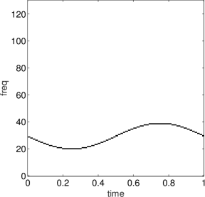
Refer to caption Refer to caption
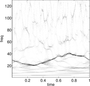
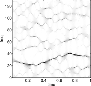
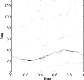
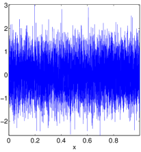
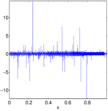
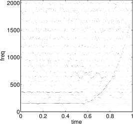
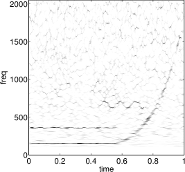
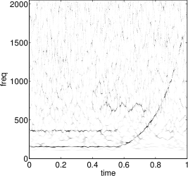
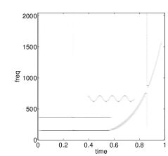
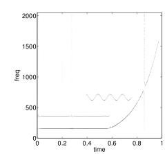
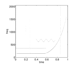
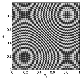
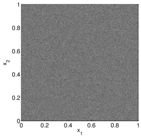
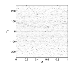
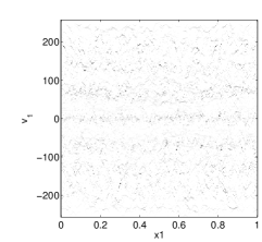
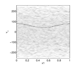
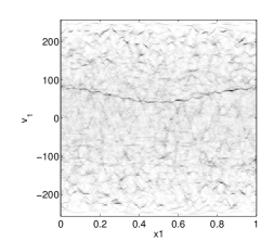
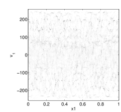
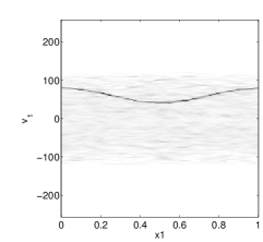
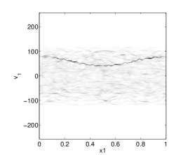
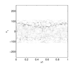
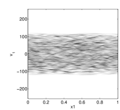
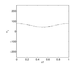
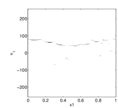
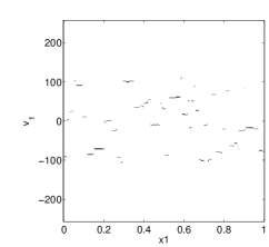
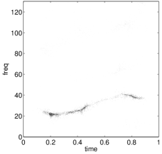
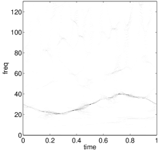
Figure 1: Top-left: The real instantaneous frequency. Top-right: The standard SSWT available in [1]. Bottom-left: The standard SSSTFT available in [1]. Bottom-right: The SSWPT with only one frame, i.e., the redundancy parameter red=1𝑟𝑒𝑑1red=1 in SynLab, which only one wave packet frame is used to compute the synchrosqueezed transform. Parameters in these transforms have been tuned for reasonably good visualization.

3.1 Implementation for better statistical stability

From the discussion in Section 2, we can summarize several observations for designing better implementation of SSTs to reduce the fluctuation of noise.

  1. 1.

    Smaller geometric parameter s𝑠s
    As we can see in the theorems for noisy data, a smaller geometric parameter s𝑠s results in a higher probability of a good estimation of the instantaneous frequency or the local wave vector via the information function vf(a,b)subscript𝑣𝑓𝑎𝑏v_{f}(a,b). Hence, in the case when noise is heavy, it is better to apply an SST with a smaller geometric parameter s𝑠s.

  2. 2.

    Highly redundant frames
    Previously in the synchrosqueezed wavelet transform (SSWT) [15], the synchrosqueezed short-time Fourier transform (SSSTFT) [37], and the synchrosqueezed wave packet transform (SSWPT) [48], various SSTs were generated from time-frequency transforms with low redundancy to obtain efficient forward and inverse transforms. However, the resultant transforms are not reliable when noise is heavy as we can see in the example in Figure 1. In this example, one single IMT f(x)=e60πi(x+0.05cos(2πx))𝑓𝑥superscript𝑒60𝜋𝑖𝑥0.052𝜋𝑥f(x)=e^{60\pi i(x+0.05\cos(2\pi x))} is embedded in white Gaussian noise with a distribution 2𝒩(0,1)2𝒩012\mathcal{N}(0,1). The signal is sampled in a time interval [0,1]01[0,1] with a sampling rate 102410241024 Hz. We apply the standard SSWT, SSSTFT in [1] and the SSWPT with s=0.75𝑠0.75s=0.75 in SynLab and visualize their results using the same discrete grid in the time-frequency domain. Although we could identify a rough curve in these results to estimate the instantaneous frequency of f(x)𝑓𝑥f(x), the accuracy is poor in some areas and there are many misleading curves coming from the noise.

    As we can see in the theory for SSTs, the accuracy of the estimation provided by the information function vf(a,b)subscript𝑣𝑓𝑎𝑏v_{f}(a,b) is essentially independent of a𝑎a and the mother wave packet w(x)𝑤𝑥w(x). This motivates us to synchrosqueeze a highly redundant time-frequency transform with over-complete samples in a𝑎a and different mother wave packets w(x)𝑤𝑥w(x). This generates many samples of estimations from a single realization of the noisy data. Averaging these estimation samples leads to a better result. It can be understood in the point of view that the contribution of IMTs to the synchrosqueezed energy distribution Tf(a,b)subscript𝑇𝑓𝑎𝑏T_{f}(a,b) will remain the same due to the coherent averaging, but the contribution of the noise will be smoothed out because of the incoherent averaging. Applying different mother wave packets is essentially the same as applying multitapers in the multitaper time-frequency reassignment in [46]. In this paper, we only focus on oversampling the variable a𝑎a and leave the design of different multidimensional mother wave packets as future work. In the numerical examples later, for a fixed geometric parameter s𝑠s, we synchrosqueeze a union of wave packet frames generated by time-frequency shifting, dilation (and rotation in multidimensional spaces). The number of frames is denoted as red𝑟𝑒𝑑red in SynLab.

  3. 3.

    Selective time-frequency coefficients
    As we can see in the proofs of previous theorems, a larger time-frequency coefficient results in a higher probability for a good estimation provided by the information function vf(a,b)subscript𝑣𝑓𝑎𝑏v_{f}(a,b). This inspires two ideas: 1) applying an adaptive time-frequency transform before synchrosqueezing; 2) only reassigning the largest coefficient in the domain where there is at most one IMT. The first idea aims at generating large coefficients while the second idea avoids incorrect reassignment as much as possible. Selecting the best coefficients to reassign, in some sense, is similar to the idea of sparse matching pursuit in a highly redundant frame, but we avoid its expensive optimization.

3.2 Numerical examples

Here we provide numerical examples to demonstrate the efficiency of the proposed implementation in Section 3.1. In all examples, we assume the given data g(x)=f(x)+e(x)𝑔𝑥𝑓𝑥𝑒𝑥g(x)=f(x)+e(x) is defined in [0,1]nsuperscript01𝑛[0,1]^{n}, where f(x)𝑓𝑥f(x) is the target signal, e(x)𝑒𝑥e(x) is white Gaussian noise with a distribution σ2𝒩(0,1)superscript𝜎2𝒩01\sigma^{2}\mathcal{N}(0,1), and n𝑛n is the dimension.

As we have seen in the theorems in Section 2, a proper threshold adaptive to the noise level after the wave packet transform is important to obtain an accurate instantaneous frequency/local wave vector estimate. We refer to [17, 18] for estimating noise level and [36] for designing thresholds for the SSWT. The generalization of these techniques for the transforms here is straightforward. In this paper, we use a small uniform threshold δ=102𝛿superscript102\delta=10^{-2} (rather than a threshold adaptive to noise level) and set σ2superscript𝜎2\sigma^{2} such that the noise is overwhelming the original signal. We refer the reader to [51, 52] for detailed implementation using these parameters.

3.2.1 Visual illustrations for statistical properties

To support the theoretical analysis in Section 2 and the proposals in Section3.1, we compare the performance of the SSWPT with different redundancy parameter red𝑟𝑒𝑑red and s=1/2+k/8𝑠12𝑘8s=1/2+k/8, where k=1𝑘1k=1, 222 and 333, in both noiseless cases and highly noisy cases.
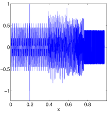
Refer to caption Refer to caption Refer to caption
Figure 2: Left: A 111D synthetic benchmark signal. It is normalized using Lsuperscript𝐿L^{\infty} norm. Middle: A noisy version generated with white Gaussian noise 0.75𝒩(0,1)0.75𝒩010.75\mathcal{N}(0,1). Right: A noisy version contaminated by an α𝛼\alpha stable random noise [2] with parameters α=1𝛼1\alpha=1, dispersion=0.9absent0.9=0.9, δ=1𝛿1\delta=1, N=8192𝑁8192N=8192. The noise is re-scaled to have a Lsuperscript𝐿L^{\infty}-norm equal to 151515 by dividing a constant factor.

One-dimensional examples:

We start with the 111D SSWPT. In some real applications, e.g., seismic data analysis [34, 52], wave-like components are only supported in a bounded domain or they have sharp changes in instantaneous frequencies. Hence, we would like to test a benchmark signal f(x)𝑓𝑥f(x) in which there is a component with a bounded support and an oscillatory instantaneous frequency, and a component with an exponential instantaneous frequency (see Figure 2). Of a special interest to test the performance of synchrosqueezed transforms for impulsive waves, a wavelet component is added in this signal at x=0.2𝑥0.2x=0.2. The synthetic benchmark signal111Prepared by Mirko van der Baan and available in [34, 40]. f(x)𝑓𝑥f(x) is defined as

f(x)=χ[0,0.6](x)f1(x)+χ[0,0.6](x)f2(x)+χ[0.6,1](x)f4(x)+χ[0.4,0.8](x)f3(x)+f5(x),𝑓𝑥subscript𝜒00.6𝑥subscript𝑓1𝑥subscript𝜒00.6𝑥subscript𝑓2𝑥subscript𝜒0.61𝑥subscript𝑓4𝑥subscript𝜒0.40.8𝑥subscript𝑓3𝑥subscript𝑓5𝑥f(x)=\chi_{[0,0.6]}(x)f_{1}(x)+\chi_{[0,0.6]}(x)f_{2}(x)+\chi_{[0.6,1]}(x)f_{4}(x)+\chi_{[0.4,0.8]}(x)f_{3}(x)+f_{5}(x),

where

f1(x)subscript𝑓1𝑥\displaystyle f_{1}(x) =\displaystyle= 0.6cos(700πx),0.6700𝜋𝑥\displaystyle 0.6\cos(700\pi x),
f2(x)subscript𝑓2𝑥\displaystyle f_{2}(x) =\displaystyle= 0.8cos(300πx),0.8300𝜋𝑥\displaystyle 0.8\cos(300\pi x),
f3(x)subscript𝑓3𝑥\displaystyle f_{3}(x) =\displaystyle= 0.7cos(1300πx+5sin(20πx)),0.71300𝜋𝑥520𝜋𝑥\displaystyle 0.7\cos(1300\pi x+5\sin(20\pi x)),
f4(x)subscript𝑓4𝑥\displaystyle f_{4}(x) =\displaystyle= sin(80π1005x/4ln(100)),80𝜋superscript1005𝑥4100\displaystyle\sin\left(\frac{80\pi 100^{5x/4}}{\ln(100)}\right),
f5(x)subscript𝑓5𝑥\displaystyle f_{5}(x) =\displaystyle= 3e50(x0.2)2cos(50(x0.2)),3superscript𝑒50superscript𝑥0.2250𝑥0.2\displaystyle 3e^{-50(x-0.2)^{2}}\cos(50(x-0.2)),

and χ(x)𝜒𝑥\chi(x) is the indicator function. f(x)𝑓𝑥f(x) is sampled in [0,1]01[0,1] with a sampling rate 819281928192 Hz and the range of instantaneous frequencies is 15016001501600150-1600 Hz. The white Gaussian noise in this example is 0.75𝒩(0,1)0.75𝒩010.75\mathcal{N}(0,1).

Although we are not aware of the optimal value of the scaling parameter s𝑠s, it is clear from Theorem 2.6 and 2.7 that the synchrosqueezed transform with a smaller s𝑠s is more suitable for noisy signals. As shown in the second and the third rows in Figure 3, in the noisy cases, the synchrosqueezed energy distribution with s=0.625𝑠0.625s=0.625 (in the first column) is better than the one with s=0.75𝑠0.75s=0.75 (in the second column), which is better than the one with s=0.875𝑠0.875s=0.875 (in the last column). This agrees with the conclusion in Theorem 2.6 and 2.7 that a smaller s𝑠s results in a higher probability to obtain a good instantaneous frequency estimate.

Another key point is that a wave packet coefficient with a larger magnitude has a higher probability to give a good instantaneous frequency estimate. A highly redundant wave packet transform would have wave packets better fitting the local oscillation of wave-like components. In another word, there would be more coefficients with large magnitudes. The resulting synchrosqueezed energy distribution has higher non-zero energy concentrating around instantaneous frequencies. This is also validated in Figure 3. The results in the third row obtained with red=16𝑟𝑒𝑑16red=16 is better than those in the second row obtained with red=1𝑟𝑒𝑑1red=1.

It is also interesting to observe that the SST with a smaller s𝑠s is better at capturing the component boundaries, e.g. at x=0.39𝑥0.39x=0.39, 0.590.590.59 and 0.770.770.77 and is more robust to an impulsive perturbation (see Figure 2 and 3 at x=0.2𝑥0.2x=0.2 and an example of α𝛼\alpha stable noise in Figure 2 and 4). Boundaries and impulse perturbations would produce frequency aliasing. The SSWPT with a smaller s𝑠s has wave packets with a smaller support in frequency and a larger support in space. Hence, it is more robust to frequency aliasing in the sense that the influence of impulsive perturbations is smoothed out and the synchrosqueezed energy of the target components might not get dispersed when it meets the frequency aliasing, as shown in Figure 4.

However, if s𝑠s is small, the instantaneous frequency estimate might be smoothed out and it is difficult to observe detailed information of instantaneous frequencies. As shown in the first row of Figure 3, when the input signal is noiseless, the synchrosqueezed transforms with s=0.75𝑠0.75s=0.75 and 0.8750.8750.875 have better accuracy than the one with s=0.625𝑠0.625s=0.625. In short, it is important to tune scaling parameters for data-dependent synchrosqueezed transforms, which has been implemented in the SynLab toolbox.

Refer to caption Refer to caption Refer to caption
Figure 3: Synchrosqueezed energy distributions with s=0.625𝑠0.625s=0.625 (left column), s=0.75𝑠0.75s=0.75 (middle column) and s=0.875𝑠0.875s=0.875 (right column). In the first row, we apply the SSWPT to clean data. In the second row, the SSWPT with a smaller redundancy is applied to the noisy data with 0.75𝒩(0,1)0.75𝒩010.75\mathcal{N}(0,1) noise in Figure 2. In the last row, a highly redundant SSWPT is applied to the same noisy data.
Refer to caption Refer to caption Refer to caption
Figure 4: Synchrosqueezed energy distributions with s=0.625𝑠0.625s=0.625 (left), s=0.75𝑠0.75s=0.75 (middle) and s=0.875𝑠0.875s=0.875 (right) using highly redundant SSWPTs. The synchrosqueezed energy with a smaller s𝑠s is smoother and the influence of impulsive noise is weaker.
Refer to caption Refer to caption
Figure 5: Left: A 222D noiseless wave-like component. Right: A noisy wave-like component generated with white Gaussian noise 5𝒩(0,1)5𝒩015\mathcal{N}(0,1).

Two-dimensional examples:

We now explore the performance of the 222D SSWPT using a single wave-like component in Figure 5. The function

f(x)=e2πi(60(x1+0.05sin(2πx1))+60(x2+0.05sin(2πx2)))𝑓𝑥superscript𝑒2𝜋𝑖60subscript𝑥10.052𝜋subscript𝑥160subscript𝑥20.052𝜋subscript𝑥2f(x)=e^{2\pi i\left(60\left(x_{1}+0.05\sin(2\pi x_{1})\right)+60\left(x_{2}+0.05\sin(2\pi x_{2})\right)\right)} (12)

is uniformly sampled in [0,1]2superscript012[0,1]^{2} with a sampling rate 512512512 Hz and is disturbed by additive white Gaussian noise 5𝒩(0,1)5𝒩015\mathcal{N}(0,1). The 222D SSWPTs with s=0.625𝑠0.625s=0.625, 0.750.750.75 and 0.8750.8750.875 are applied to this noisy example and their results are shown in Figure 6. Since the synchrosqueezed energy distribution Tf(v1,v2,x1,x2)subscript𝑇𝑓subscript𝑣1subscript𝑣2subscript𝑥1subscript𝑥2T_{f}(v_{1},v_{2},x_{1},x_{2}) of an image is a function in 4superscript4\mathbb{R}^{4}, we fix x2=0subscript𝑥20x_{2}=0, stack the results in v2subscript𝑣2v_{2}, and visualize Tf(v1,v2,x1,0)𝑑v2subscriptsubscript𝑇𝑓subscript𝑣1subscript𝑣2subscript𝑥10differential-dsubscript𝑣2\int_{\mathbb{R}}T_{f}(v_{1},v_{2},x_{1},0)dv_{2}. The results in Figure 6 again validate the theoretical conclusion in Theorem 2.8 that a smaller scaling parameter s𝑠s and a higher redundancy yield to a better SST for noisy data.

It is interesting that a band-limited SST can also provide better statistical stability if the range of instantaneous frequencies/local wave vectors is known a priori. Let us justify this idea with the follow example. We apply the band-limited SSWPT to the 222D noisy image in Figure 6 and present the results in the last row of Figure 6. Comparing to the results in the second row of Figure 6, the band-limited SSWPT clearly outperforms the original SSWPT.
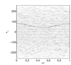
Refer to caption Refer to caption Refer to caption
Figure 6: Stacked synchrosqueezed energy distribution Tf(v1,v2,x1,0)𝑑v2subscriptsubscript𝑇𝑓subscript𝑣1subscript𝑣2subscript𝑥10differential-dsubscript𝑣2\int_{\mathbb{R}}T_{f}(v_{1},v_{2},x_{1},0)dv_{2} of the noisy 222D signal in Figure 5. From left to right, s=0.625𝑠0.625s=0.625, 0.750.750.75 and 0.8750.8750.875. From top to bottom: red=1𝑟𝑒𝑑1red=1, red=10𝑟𝑒𝑑10red=10, and red=10𝑟𝑒𝑑10red=10 with a restricted frequency band from 202020 to 120120120 Hz.

Component test

Here we present an example to validate the last observation in Section 3.1. Suppose we look at a region in the time-frequency or phase space domain and we know there might be only one IMT in this region. This assumption is reasonable because after the SST people might be interested in the synchrosqueezed energy in a particular region: is this corresponding to a component or just heavy noise? A straightforward solution is that, at each time or space grid point, we only reassign those coefficients with the largest magnitude. By Theorem 2.8, if there is an IMT, we can obtain a sketch of its instantaneous frequency or local wave vector with a high probability. If there was only noise, we would obtain random reassigned energy with a high probability. Using this idea, we apply the band-limited SSWPT with s=0.625𝑠0.625s=0.625 and red=10𝑟𝑒𝑑10red=10 to a noisy version of the image in Figure 5 left. From left to right, Figure 7 shows the results of a noisy image (12) with 5𝒩(0,1)5𝒩015\mathcal{N}(0,1) noise, a noisy image (12) with 10𝒩(0,1)10𝒩0110\mathcal{N}(0,1) noise, and an image with only noise, respectively. A reliable sketch of the local wave vector is still visible even if the input image is highly noisy.
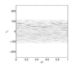
Refer to caption Refer to caption Refer to caption
Figure 7: Top row: The synchrosqueezed energy distribution of the highly redundant band-limited SSWPT with a frequency band 202020 to 120120120 Hz. Bottom row: reassigned wave packet coefficients with the largest magnitude at a space location. Left column: 5𝒩(0,1)5𝒩015\mathcal{N}(0,1) noise. Middle column: 10𝒩(0,1)10𝒩0110\mathcal{N}(0,1) noise. Right column: noise only.

3.2.2 Quantitative performance analysis

We quantitatively analyze the performance of the highly redundant SSWPT and compare it with other methods in this subsection in terms of statistical stability and computational efficiency. Let us revisit the wave-like component in Figure 1, where

f(x)=e60πi(x+0.05cos(2πx))𝑓𝑥superscript𝑒60𝜋𝑖𝑥0.052𝜋𝑥f(x)=e^{60\pi i(x+0.05\cos(2\pi x))}

is sampled in [0,1]01[0,1] with a sampling rate 102410241024 Hz. Its instantaneous frequency is q(x)=30(10.1πsin(2πx))𝑞𝑥3010.1𝜋2𝜋𝑥q(x)=30(1-0.1\pi\sin(2\pi x)). Let g=f+e𝑔𝑓𝑒g=f+e be the noisy data, where e𝑒e is white Gaussian noise with a distribution σ2𝒩(0,1)superscript𝜎2𝒩01\sigma^{2}\mathcal{N}(0,1). To measure noise, we introduce the following signal-to-noise ratio (SNR) of the input data g=f+e𝑔𝑓𝑒g=f+e:

SNR[dB](g)=10log10(Var(f)Var(e)).SNRdelimited-[]𝑑𝐵𝑔10subscript10Var𝑓Var𝑒\text{SNR}[dB](g)=10\log_{10}\left(\frac{\text{Var}(f)}{\text{Var}(e)}\right).

An ideal time-frequency distribution of f(x)𝑓𝑥f(x) is a function D(v,x)𝐷𝑣𝑥D(v,x) such that D(v,x)=δ(vq(x))𝐷𝑣𝑥𝛿𝑣𝑞𝑥D(v,x)=\delta(v-q(x)), where δ(v)𝛿𝑣\delta(v) is a Dirac delta function of v𝑣v. To quantify the numerical performance of various methods, we introduce the Earth mover’s distance (EMD) [29, 30, 31] to measure the distance between a resultant time-frequency distribution T(v,x)𝑇𝑣𝑥T(v,x) and the ideal distribution D(v,x)𝐷𝑣𝑥D(v,x). At each x𝑥x, after the discretization and normalization of T(v,x)𝑇𝑣𝑥T(v,x), we obtain a 111D discrete distribution T~(v,x)~𝑇𝑣𝑥\tilde{T}(v,x). Similarly, we compute the discrete version D~(v,x)~𝐷𝑣𝑥\tilde{D}(v,x) of D(v,x)𝐷𝑣𝑥D(v,x). At each x𝑥x, we compute the 111D EMD between T~(v,x)~𝑇𝑣𝑥\tilde{T}(v,x) and D~(v,x)~𝐷𝑣𝑥\tilde{D}(v,x). The average EMD at all x𝑥x is defined as the distance (also denoted as EMD) between T(v,x)𝑇𝑣𝑥T(v,x) and D(v,x)𝐷𝑣𝑥D(v,x) in this paper. A smaller EMD means a better time-frequency concentration to the ground true instantaneous frequency and fewer noise fluctuations.
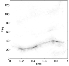
Refer to caption Refer to caption Refer to caption
Figure 8: Left and middle: The multitaper time-frequency reassignment using an arithmetic mean (MRSA) and a geometric mean (MRSG) with 101010 tapers. Right: The highly redundant SSWPT with s=0.75𝑠0.75s=0.75 and red=10𝑟𝑒𝑑10red=10.

First, we compare the performance of the SSWPT with different redundancy parameters red𝑟𝑒𝑑red for noisy data with different SNRs. We compare the EMD between their resultant time-frequency distributions and the ideal one. Figure 9 (top-left) shows the EMD as functions in the variable of red𝑟𝑒𝑑red. The EMD functions decrease fast when the red𝑟𝑒𝑑red increases to 101010. All the SSWPTs with red10𝑟𝑒𝑑10red\geq 10 have almost the same efficiency.

Second, we compare the performance of the SSWPT with the same redundancy parameters red=10𝑟𝑒𝑑10red=10 but different geometric scaling parameter s𝑠s for noisy data with different noise level, e.g. σ2superscript𝜎2\sigma^{2} ranging from 00 to 444, i.e., SNR from \infty to 1515-15. We compare the EMD between their resultant time-frequency distributions and the ideal one. Figure 9 (top-right) shows the EMD as functions in the variable of σ2superscript𝜎2\sigma^{2} for different s𝑠s. It shows that when the data is clean, the SSWPT with s=1𝑠1s=1, which is essentially the SSWT with high redundancy, has the best performance. However, once the data is noisy, the SSWPT with s=0.75𝑠0.75s=0.75 has the best overall performance. This observation agrees with our theorems in Section 2. If s𝑠s is larger, the instantaneous frequency estimation is more accurate if there is no noise. But the probability for a good estimation is smaller if there is noise. If s𝑠s is smaller , the estimation accuracy is worse but the probability for a good estimation is higher. In theory, it is interesting to find an optimal s𝑠s that makes a good balance. In practice, a heuristic choice for the optimal s𝑠s is 0.750.750.75.

Third, we compare the performance of the standard SSWT, SSSTFT in [1] and the highly redundant SSWPT. Again, we choose the parameters in the example of Figure 1 because they result in good visualization of time-frequency distribution. These transforms are applied to noisy data with different noise level. We compare the EMD between their resultant time-frequency distributions and the ideal one. The comparison is shown in Figure 9 (bottom-left). The highly redundant SSWPT has better time-frequency concentration than the standard SSWT and SSSTFT in all examples, even if in the noiseless case.

Finally, we compare the multitaper time-frequency reassignment using an arithmetic mean (MRSA) and a geometric mean (MRSG) in[46] with the highly redundant SSWPT. A MATLAB package of the MRSA and the MRSG is available on the authors’ homepage. The time-frequency distribution of these three methods are visualized in Figure 8. We visualize their results using the same discrete grid in the time-frequency domain. To make a fair comparison, the number of tapers are chosen to be 101010 for the MRSA and the MRSG, and the redundancy parameter red𝑟𝑒𝑑red is 101010 for the SSWPT with s=0.75𝑠0.75s=0.75. For one realization of this experiment, the running time for the MRSA or the MRSG is 155.13155.13155.13 seconds, while the running time for the SSWPT is only 0.430.430.43 seconds. A visual inspection of Figure 8 shows that the SSWPT also outperforms the MRSA and the MRSG: clear spectral energy at the boundary and better time-frequency concentration. To quantify this comparison, we apply the EMD again and the results are shown in Figure 9 (bottom-right). In most cases, the SSWPT with s=0.75𝑠0.75s=0.75 gives a smaller EMD. When σ2superscript𝜎2\sigma^{2} is near 444, i.e., the SNR is near 1515-15, the MRSG with 101010 tapers and the SSWPT have comparable performance.
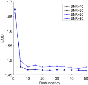
Refer to caption Refer to caption
Figure 9: Top-left: The EMD as functions in the variable of red𝑟𝑒𝑑red for different SNRs. Bottom-left: Comparison of the standard SSWT, SSSTFT and the SSWPT. Bottom-right: Comparison of the multitaper time-frequency reassignment (the numbers of tapers are 555 and 101010) and the SSWPT. Data plotted above is the averaging of 202020 independent realizations.

4 Conclusion

In theory, the statistical analysis in this paper has analyzed the statistical properties of a wide range of compactly supported synchrosqueezed transforms in multidimensional spaces, considering zero mean stationary Gaussian random process and small perturbation. Guided by these properties, this paper has presented several approaches to improve the performance of these synchrosqueezed transforms under heavy noise. A MATLAB package SynLab for these algorithms is available at https://github.com/HaizhaoYang/SynLab.

Acknowledgments. This work was partially supported by the National Science Foundation under award DMS-0846501 and the U.S. Department of Energy’s Advanced Scientific Computing Research program under award DE-FC02-13ER26134/DE-SC0009409 for Lexing Ying. H. Yang is also supported by a AMS Simons travel grant. He thanks Jean-Baptiste Tary and Mirko van der Baan for the discussion of benchmark signals, thanks Lexing Ying, Charles K. Chui, Jianfeng Lu and Segey Fomel for the discussion of the implementation and the application of synchrosqueezed transforms.

References

  • [1] https://sites.google.com/site/hautiengwu/home/download.
  • [2] http://users.ece.utexas.edu/~bevans/projects/rfi/software/.
  • [3] F. Auger and P. Flandrin. Improving the readability of time-frequency and time-scale representations by the reassignment method. Signal Processing, IEEE Transactions on, 43(5):1068 –1089, 1995.
  • [4] F. Auger, P. Flandrin, Y.-T. Lin, S. McLaughlin, S. Meignen, T. Oberlin, and H. tieng Wu. Time-frequency reassignment and synchrosqueezing: An overview. Signal Processing Magazine, IEEE, 30(6):32–41, Nov 2013.
  • [5] M. Bayram and R. Baraniuk. Multiple window time-frequency analysis. In Time-Frequency and Time-Scale Analysis, 1996., Proceedings of the IEEE-SP International Symposium on, pages 173–176, Jun 1996.
  • [6] B. Boashash and S. Member. Estimating and interpreting the instantaneous frequency of a signal. In Proceedings of the IEEE, pages 520–538, 1992.
  • [7] E. J. Candès, P. R. Charlton, and H. Helgason. Detecting highly oscillatory signals by chirplet path pursuit. Applied and Computational Harmonic Analysis, 24(1):14 – 40, 2008.
  • [8] E. Chassande-Mottin, F. Auger, and P. Flandrin. Time-frequency/time-scale reassignment. In Wavelets and signal processing, Appl. Numer. Harmon. Anal., pages 233–267. Birkhäuser Boston, Boston, MA, 2003.
  • [9] E. Chassande-Mottin, I. Daubechies, F. Auger, and P. Flandrin. Differential reassignment. Signal Processing Letters, IEEE, 4(10):293 –294, 1997.
  • [10] E. Chassande-Mottin, P. Flandrin, and F. Auger. On the statistics of spectrogram reassignment vectors. Multidimensional Systems and Signal Processing, 9(4):355–362, 1998.
  • [11] E. Chassande-Mottin and A. Pai. Best chirplet chain: Near-optimal detection of gravitational wave chirps. Physical Review D, 73(4), 2006.
  • [12] Y.-C. Chen, M.-Y. Cheng, and H.-T. Wu. Non-parametric and adaptive modelling of dynamic periodicity and trend with heteroscedastic and dependent errors. Journal of the Royal Statistical Society: Series B (Statistical Methodology), 76(3):651–682, 2014.
  • [13] C. K. Chui, Y.-T. Lin, and H.-T. Wu. Real-time dynamics acquisition from irregular samples – with application to anesthesia evaluation. Analysis and Applications, Accepted.
  • [14] M. Clausel, T. Oberlin, and V. Perrier. The monogenic synchrosqueezed wavelet transform: a tool for the decomposition/demodulation of am–fm images. Applied and Computational Harmonic Analysis, 39(3):450 – 486, 2015.
  • [15] I. Daubechies, J. Lu, and H.-T. Wu. Synchrosqueezed wavelet transforms: an empirical mode decomposition-like tool. Appl. Comput. Harmon. Anal., 30(2):243–261, 2011.
  • [16] I. Daubechies and S. Maes. A nonlinear squeezing of the continuous wavelet transform based on auditory nerve models. In Wavelets in Medicine and Biology, pages 527–546. CRC Press, 1996.
  • [17] D. L. Donoho. De-noising by soft-thresholding. IEEE Trans. Inf. Theor., 41(3):613–627, may 1995.
  • [18] D. L. Donoho and J. M. Johnstone. Ideal spatial adaptation by wavelet shrinkage. Biometrika, 81(3):425–455, 1994.
  • [19] S. Fomel. Seismic data decomposition into spectral components using regularized nonstationary autoregression. Geophysics, 78(6):O69–O76, 2013.
  • [20] G. Fraser and B. Boashash. Multiple window spectrogram and time-frequency distributions. In Acoustics, Speech, and Signal Processing, 1994. ICASSP-94., 1994 IEEE International Conference on, volume iv, pages IV/293–IV/296 vol.4, Apr 1994.
  • [21] R. G. Gallager. Circularly-symmetric gaussian random vectors. preprint, 2008.
  • [22] R. Herrera, J. Han, and M. van der Baan. Applications of the synchrosqueezing transform in seismic time-frequency analysis. Geophysics, 79(3):V55–V64, 2014.
  • [23] W. Huang, Z. Shen, N. E. Huang, and Y. C. Fung. Engineering analysis of biological variables: An example of blood pressure over 1 day. Proc. Natl. Acad. Sci., 95, 1998.
  • [24] H.-H. Kuo. White noise distribution theory. Probability and stochastics series. CRC Press, Boca Raton (USA), 1996.
  • [25] C. Li and M. Liang. A generalized synchrosqueezing transform for enhancing signal time–frequency representation. Signal Processing, 92(9):2264 – 2274, 2012.
  • [26] J. Lu, B. Wirth, and H. Yang. Combining 2D synchrosqueezed wave packet transform with optimization for crystal image analysis. arXiv:1501.06254, 2015.
  • [27] F. Neeser and J. Massey. Proper complex random processes with applications to information theory. Information Theory, IEEE Transactions on, 39(4):1293–1302, Jul 1993.
  • [28] T. Oberlin, S. Meignen, and V. Perrier. Second-order synchrosqueezing transform or invertible reassignment? towards ideal time-frequency representations. Signal Processing, IEEE Transactions on, 63(5):1335–1344, March 2015.
  • [29] O. Pele and M. Werman. A linear time histogram metric for improved sift matching. In D. Forsyth, P. Torr, and A. Zisserman, editors, Computer Vision – ECCV 2008, volume 5304 of Lecture Notes in Computer Science, pages 495–508. Springer Berlin Heidelberg, 2008.
  • [30] O. Pele and M. Werman. Fast and robust earth mover’s distances. In Computer Vision, 2009 IEEE 12th International Conference on, pages 460–467, Sept 2009.
  • [31] S. Peleg, M. Werman, and H. Rom. A unified approach to the change of resolution: space and gray-level. Pattern Analysis and Machine Intelligence, IEEE Transactions on, 11(7):739–742, Jul 1989.
  • [32] B. Picinbono. On instantaneous amplitude and phase of signals. IEEE Trans. Signal Processing, pages 552–560, 1997.
  • [33] H. M. Singer and I. Singer. Analysis and visualization of multiply oriented lattice structures by a two-dimensional continuous wavelet transform. Physical Review E, 74:031103, 2006.
  • [34] J. B. Tary, R. H. Herrera, J. Han, and M. van der Baan. Spectral estimation-What is new? What is next? Review of Geophysics, 52(4):723–749, Dec. 2014.
  • [35] M. Taylor. Random fields: stationarity, ergodicity, and spectral behavior, http://www.unc.edu/math/Faculty/met/rndfcn.pdf.
  • [36] G. Thakur, E. Brevdo, N. S. Fučkar, and H.-T. Wu. The synchrosqueezing algorithm for time-varying spectral analysis: robustness properties and new paleoclimate applications. Signal Processing, 93(5):1079–1094, 2013.
  • [37] G. Thakur and H.-T. Wu. Synchrosqueezing-based recovery of instantaneous frequency from nonuniform samples. SIAM J. Math. Analysis, 43(5):2078–2095, 2011.
  • [38] D. Thomson. Spectrum estimation and harmonic analysis. Proceedings of the IEEE, 70(9):1055–1096, Sept 1982.
  • [39] A. Van Den Bos. The multivariate complex normal distribution – a generalization. Information Theory, IEEE Transactions on, 41(2):537–539, Mar 1995.
  • [40] M. van der Baan. http://www.ualberta.ca/~vanderba/ftp/benchmark_signals.zip.
  • [41] A. D. Veltcheva. Wave and group transformation by a hilbert spectrum. Coastal Engineering Journal, 44(4), 2002.
  • [42] H.-T. Wu. Instantaneous frequency and wave shape functions (i). Applied and Computational Harmonic Analysis, 35(2):181 – 199, 2013.
  • [43] H.-T. Wu, Y.-H. Chan, Y.-T. Lin, and Y.-H. Yeh. Using synchrosqueezing transform to discover breathing dynamics from ECG signals. Applied and Computational Harmonic Analysis, 36(2):354 – 359, 2014.
  • [44] H.-T. Wu, S.-S. Hseu, M.-Y. Bien, Y. R. Kou, and I. Daubechies. Evaluating physiological dynamics via synchrosqueezing: Prediction of ventilator weaning. IEEE Transactions on Biomedical Engineering, 61(3):736–744, March 2014.
  • [45] Z. Wu, N. E. Huang, and X. Chen. Some considerations on physical analysis of data. Advances in Adaptive Data Analysis, 3(1-2):95–113, 2011.
  • [46] J. Xiao and P. Flandrin. Multitaper time-frequency reassignment for nonstationary spectrum estimation and chirp enhancement. Signal Processing, IEEE Transactions on, 55(6):2851–2860, June 2007.
  • [47] H. Yang. Oscillatory data analysis and fast algorithms for integral operators. PhD thesis, Stanford University, 2015. This dissertation is online at: http://purl.stanford.edu/fq061ny3299 or http://web.stanford.edu/~haizhao/publications/ThesisHaizhao.pdf.
  • [48] H. Yang. Synchrosqueezed wave packet transforms and diffeomorphism based spectral analysis for 1d general mode decompositions. Applied and Computational Harmonic Analysis, 39(1):33 – 66, 2015.
  • [49] H. Yang, J. Lu, W. Brown, I. Daubechies, and L. Ying. Quantitative canvas weave analysis using 2-D synchrosqueezed transforms: Application of time-frequency analysis to art investigation. Signal Processing Magazine, IEEE, 32(4):55–63, July 2015.
  • [50] H. Yang, J. Lu, and L. Ying. Crystal image analysis using 2D synchrosqueezed transforms. Multiscale Modeling & Simulation. A SIAM Interdisciplinary Journal, 2015.
  • [51] H. Yang and L. Ying. Synchrosqueezed wave packet transform for 2d mode decomposition. SIAM Journal on Imaging Sciences, 6(4):1979–2009, 2013.
  • [52] H. Yang and L. Ying. Synchrosqueezed curvelet transform for two-dimensional mode decomposition. SIAM Journal on Mathematical Analysis, 46(3):2052–2083, 2014.