A relative Grace Theorem for complex polynomials

Abstract.

We study the pullback of the apolarity invariant of complex polynomials in one variable under a polynomial map on the complex plane. As a consequence, we obtain variations of the classical results of Grace and Walsh in which the unit disk, or a circular domain, is replaced by its image under the given polynomial map.

Introduction

Let $f(z)=a_{0}+a_{1}z+\ldots+a_{n}z^{n}$ and $g(z)=b_{0}+b_{1}z+\ldots+b_{n}z^{n}$ be two polynomials with complex coefficients and degrees less than or equal to $n$. The only joint invariant under affine substitutions which is linear in the coefficients is

$$[f,g]_{n}=a_{0}b_{n}-\frac{1}{n}a_{1}b_{n-1}+\frac{1}{\binom{n}{2}}a_{2}b_{n-2}+\ldots+(-1)^{n}a_{n}b_{0}.$$

The two polynomials are called apolar if $[f,g]_{n}=0$. Apolarity provides the ground for the study of the simplest type of invariant, generalizing in higher degree the notion of harmonic quadrics. The geometric implications of apolarity are surprising and multifold, see for instance [GY03]. A celebrated result due to Grace and Heawood asserts that the complex zeros of two apolar polynomials cannot be separated by a circle or a straight line. As a matter of fact, this zero location property is equivalent to apolarity [Di38]. An array of independent proofs of Grace’s theorem, as the result is named nowadays, are known (see [Ho54, Ma66, RS02, Sz22]). The common technical ingredient of these proofs is a lemma of Laguerre and induction. Notable is also the coincidence, up to a conjugation in the second argument, of the apolarity invariant and Fischer’s inner product:

$$\langle f,g\rangle_{n}=\sum_{k=0}^{n}\frac{1}{\binom{n}{k}}a_{k}\overline{b_{k}},$$

well known for identifying the adjoint of complex differentiation with the multiplication by the variable [Fi17].

It is natural and convenient to symmetrize the polynomials $f$ and $g$ and interpret both apolarity and Fischer inner products in terms of the roots of these polynomials. In this direction an observation due to Walsh establishes a powerful equivalent statement to Grace’s theorem, known as the Walsh Coincidence Theorem: If a monic polynomial $f$ of degree $n$ has no zeros in a circular domain $D$ (that is a disc, complement of a disk, a half-space, open or closed), then its symmetrization has no zeros in $D^{n}$, [Ho54, Ma66, RS02, Sz22]. In its turn, Walsh’s theorem explains and offers a natural framework for a series of polynomial inequalities, in one or several variables [Be26, CS35, Ho54].

The aim of the present note is to study the pull-back of the apolarity invariant by a polynomial mapping $q$ of degree $d$. It turns out that the pull-back form can be represented on the original space of polynomials of degree $n$ by an invertible linear operator $T_{q,n}$:

$$[f\circ q,g\circ q]_{nd}=[T_{q,n}f,g]_{n}.$$

At the geometric level, the pull back is transformed into push-forward by the ramified cover map $q$. For a circular domain $D$, we distinguish between the set theoretic image $q(D)$ and the full push-forward $q_{\circ}(D)$ which consists of all points in $q(D)$ having the full fiber contained in $D$. Relative $q$-versions of the theorems of Grace and Walsh follow easily, for instance: If two polynomials $f$ and $g$ are $q-apolar$ and all zeros of $f$ are contained in $q_{\circ}(D)$, then $g$ has a zero in $q(D)$. As expected, the $q$-version of the Walsh Coincidence Theorem has non-trivial consequences in the form of polynomial inequalities for symmetric polynomials of several variables. To be more specific we prove below that a majorization on the diagonal of $q(D)$ is transmitted, with the same constant, to the polydomain $q_{\circ}(D)^{n}$.

The operator $T_{q,n}$ representing the $q$-apolarity form is complex symmetric, in the sense of [GPP14], and as a consequence the eigenfunctions of its modulus are doubly orthogonal, both in the Fischer norm, and with respect to the apolarity bilinear form. In particular the zeros of these polynomials cannot be separated by higher degree algebraic sets deduced from the boundaries of $q(D)$, respectively $q_{\circ}(D)$.

The idea of providing a more flexible version of Grace’s theorem also relates to recent work of B. and H. Sendov in [Se14], which is concerned with finding minimal domains satisfying the statement of Grace’s theorem for a given polynomial.

This paper is structured as follows: Section 1 contains notation, preliminaries and some of the classical results. In Section 2, we discuss polynomial images of circular domains. Section 3 contains the core results on symmetrization and pullback and the relative versions of the theorems of Grace and Walsh. Section 4 concerns the study of skew-eigenfunctions of the symmetrization operator $T_{q,n}$ in the sense of [GPP14].

Acknowledgements. We would like to thank one of the referees for helpful comments. Daniel Plaumann was partially supported by a Research Fellowship of the Nanyang Technological University.

1. Preliminaries

We write $\mathbb{C}[z]_{n}$ for the space of complex polynomials in $z$ of degree at most $n$.

1.1.

For $f=\sum_{k=0}^{n}a_{k}z^{k}\in\mathbb{C}[z]_{n}$, the symmetrization of $f$ in degree $n$ is the polynomial in $n$ variables $y_{1},\dots,y_{n}$ defined by

$$\operatorname{Sym}_{n}(f)=\sum_{k=0}^{n}\frac{a_{k}}{\binom{n}{k}}\sigma_{k}(y_{1},\dots,y_{n}),$$

where $\sigma_{k}(y_{1},\dots,y_{n})$ is the elementary symmetric polynomial of degree $k$ in $y_{1},\dots,y_{n}$. The symmetrization is the unique multiaffine symmetric polynomial of degree at most $n$ in $y_{1},\dots,y_{n}$ with the property

$$\operatorname{Sym}_{n}(f)(z,\dots,z)=f(z).$$

To verify uniqueness, just note that a multiaffine symmetric polynomial of degree at most $n$ in $y_{1},\dots,y_{n}$ is necessarily of the form $\sum_{k=0}^{n}b_{k}\sigma_{k}(y_{1},\dots,y_{n})$.

1.2.

For $f=\sum_{k=0}^{n}a_{k}z^{k}\in\mathbb{C}[z]_{n}$, we write

$$f^{\vee}=f(-z)=\sum\nolimits_{k=0}^{n}(-1)^{k}a_{k}z^{k}$$

$$f^{\#}=z^{n}\overline{f\bigl{(}1/\overline{z}\bigr{)}}=\sum\nolimits_{k=0}^{n}\overline{a_{n-k}}z^{k}$$

Observe that $(fg)^{\#}=f^{\#}g^{\#}$ and $\bigl{(}\prod_{k=1}^{n}(z-\lambda_{k})\bigr{)}^{\#\vee}=\prod_{k=1}^{n}(1+\overline{\lambda_{k}}z)$. Note also that the definition of $f^{\#}$ depends on $n$. Even if $a_{n}=0$, so that $f$ is of degree less than $n$, it is understood that $f^{\#}$ is defined as above whenever we take $f\in\mathbb{C}[z]_{n}$.

1.3.

The Fischer inner product is the Hermitian inner product on $\mathbb{C}[z]_{n}$ given by

$$\langle f,g\rangle_{n}=\sum_{k=0}^{n}\frac{1}{\binom{n}{k}}a_{k}\overline{b_{k}}$$

for $f(z)=\sum_{k=0}^{n}a_{n}z^{n}$ and $g(z)=\sum_{k=0}^{n}b_{n}z^{n}$. The following hold for all $f\in\mathbb{C}[z]_{n}$.

1. $\langle z^{k},z^{l}\rangle_{n}=\delta_{k,l}/\binom{n}{k}$ for $k,l=0,\dots,n$;
   

2. $\langle f,g^{\#\vee}\rangle_{n}=(-1)^{n}\langle g,f^{\#\vee}\rangle_{n}$ for all $g\in\mathbb{C}[z]_{n}$;
   

3. $\langle zg,f\rangle_{n}=\frac{1}{n}\langle g,f^{\prime}\rangle_{n-1}$ for all $g\in\mathbb{C}[z]_{n-1}$;
   

4. $f(\lambda)=\langle f,(1+\overline{\lambda}z)^{n}\rangle_{n}$ for all $\lambda\in\mathbb{C}$;
   

5. $\operatorname{Sym}_{n}(f)(y_{1},\dots,y_{n})=\langle f,\prod_{k=1}^{n}(1+\overline{y_{k}}z)\rangle_{n}=\langle f,(\prod_{k=1}^{n}(z-y_{k}))^{\#\vee}\rangle$.

Proof.

(1)—(4) are checked directly. To verify (5), expanding the product $\prod_{k=0}^{n}(1+\overline{y_{k}}z)=\sum_{k=0}^{n}\overline{\sigma_{k}(y_{1},\dots,y_{n})}z^{k}$ shows that

$$\bigl{\langle}f,\prod\nolimits_{k=1}^{n}(1+\overline{y_{k}}z)\bigl{\rangle}_{n} =\bigl{\langle}\sum\nolimits_{k=0}^{n}a_{k}z^{k},\sum\nolimits_{k=0}^{n}\overline{\sigma_{k}(y_{1},\dots,y_{n})}z^{k}\bigl{\rangle}_{n}$$

$$=\sum\nolimits_{k=0}^{n}\frac{1}{\binom{n}{k}}a_{k}\sigma_{k}(y_{1},\dots,y_{n})=\operatorname{Sym}_{n}(f).\qed$$

1.4.

For $f,g\in\mathbb{C}[z]_{n}$, we define

$$[f,g]_{n}=\langle f,g^{\#\vee}\rangle_{n}.$$

Note that if $g$ is monic of degree $n$ with zeros $\mu_{1},\dots,\mu_{n}$, then

$$[f,g]_{n}=\operatorname{Sym}_{n}(f)(\mu_{1},\dots,\mu_{n}).$$

by 1.3(5). The form $[-,-]_{n}$ is bilinear and non-degenerate and, by 1.3(2), satisfies

$$[f,g]_{n}=(-1)^{n}[g,f]_{n}.$$

If $[f,g]_{n}=0$, then $f$ and $g$ are called apolar.

A circular domain is an open or closed disk or halfspace in $\mathbb{C}$, or the complement of any such set. We use $\mathbb{D}$ to denote the open unit disk.

Theorem 1.5 (Walsh).

If $D\subset\mathbb{C}$ is a circular domain and $f\in\mathbb{C}[z]_{n}$ is monic without zeros in $D$, then $\operatorname{Sym}_{n}(f)$ has no zeros in $D^{n}$.

Since the complement of a circular domain is again a circular domain, an equivalent statement of Walsh’s theorem is

Theorem (Walsh).

Let $D\subset\mathbb{C}$ be a circular domain. If $f\in\mathbb{C}[z]_{n}$ is monic with all zeros in $D$ and $(y_{1},\dots,y_{n})\in\mathbb{C}^{n}$ is a zero of $\operatorname{Sym}_{n}(f)$, then $y_{k}\in D$ for some $k\in\{1,\dots,n\}$.

See Hörmander [Ho54] (or [Ma66, RS02, Sz22]) for the proof.

Corollary 1.6 (Grace’s Theorem).

Let $D\subset\mathbb{C}$ be a circular domain and let $f,g\in\mathbb{C}[z]$ be apolar polynomials of the same degree. If all zeros of $f$ are contained in $D$, then $g$ has at least one zero in $D$.

Proof.

Let $n=\deg(f)=\deg(g)$. Without loss of generality, we may assume that $g$ is monic and write $g=\prod_{k=1}^{n}(z-\mu_{k})$. Then

$$[f,g]_{n}=\operatorname{Sym}_{n}(f)(\mu_{1},\dots,\mu_{n})$$

by 1.4. By Walsh’s theorem, at least one of $\mu_{1},\dots,\mu_{n}$ must lie in $D$, as claimed. ∎

2. Polynomial images of circular domains

Let $D\subset\mathbb{C}$ be a circular domain and let $q\in\mathbb{C}[z]$ be a monic polynomial of degree $d$. We want to understand how Walsh’s and Grace’s theorem transform under the map $q\colon\mathbb{C}\to\mathbb{C}$. We will use the following notation:

$$q_{\circ}(D)\;=\;\bigl{\{}u\in\mathbb{C}\>|\>q^{-1}(u)\subset D\bigr{\}}.$$

The set $q_{\circ}(D)$ is semialgebraic and its boundary is contained in the real algebraic curve $q(\partial D)$. Since the complement of a circular domain is a circular domain, the set $q_{\circ}(D)$ is the complement of the image of a circular domain, namely

$$q(\mathbb{C}\setminus D)=\mathbb{C}\setminus q_{\circ}(D)\quad\text{and}\quad q_{\circ}(\mathbb{C}\setminus D)=\mathbb{C}\setminus q(D).$$

Example 2.1.

Let $q=z^{2}+\beta z+\gamma$. Two points $z,w\in\mathbb{C}$ have the same image under $q$ if and only if $z+w=-\beta$. This implies

$$q^{-1}(q_{\circ}(D))=\bigl{\{}z\in D\>|\>-(z+\beta)\in D\bigr{\}}=D\cap-(D+\beta).$$

and $q_{\circ}(D)$ is the image of that region under $q$. In particular, if $D=\mathbb{D}$ is the open unit disk, then $q_{\circ}(\mathbb{D})$ is non-empty if and only if $|\beta|<2$.

For example, take $q=z^{2}+\frac{1}{2}z$. The image of the unit circle under $q$ is the real quartic curve $\{z=x+iy\>|\>u(x,y)=0\}$ in the complex plane, where

$$u(x,y)=4x^{4}+4y^{4}+8x^{2}y^{2}-9x^{2}-9y^{2}-2x+3.$$

The preimage of this curve under $q$ consists of the unit circle and the shifted unit circle $\{z\in\mathbb{C}\>|\>|z+\frac{1}{2}|=1\}$. The region $q_{\circ}(\mathbb{D})$ and its preimage are shown in Fig. 1.

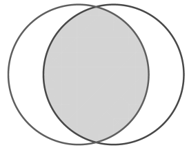
$\xrightarrow{\ \ \ q\ \ \ }$

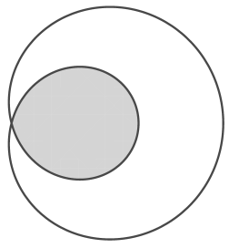
Figure 1. The region $q_{\circ}(\mathbb{D})$ and its preimage for $q=z^{2}+\frac{1}{2}z$

Example 2.2.

Consider the cubic polynomial $q=z^{3}+\frac{1}{2}z$. The image of the unit circle under $q$ is the real sextic curve $\{z=x+iy\>|\>h(x,y)=0\}$ given by

$$u(x,y)=16x^{6}+48x^{4}y^{2}-52x^{4}+48x^{2}y^{4}-104x^{2}y^{2}+40x^{2}+16y^{6}-52y^{4}+48y^{2}-9$$

shown on the right-hand side of Figure 2. The preimage of this curve under $q$ has two real components, the unit circle and a curve of degree $8$ given by the vanishing of the polynomial

$$v(x,y)=\; 16x^{8}+16x^{6}+64x^{6}y^{2}+96x^{4}y^{4}-16x^{4}y^{2}+8x^{4}+64x^{2}y^{6}-80x^{2}y^{4}$$

$$-16x^{2}y^{2}-28x^{2}+16y^{8}-48y^{6}+40y^{4}-12y^{2}+9.$$

This curve is shown on the left of Figure 2. Together with the unit circle, it bounds the region $q^{-1}(q_{\circ}(\mathbb{D}))$.

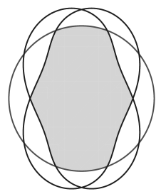
$\xrightarrow{\ \ \ q\ \ \ }$

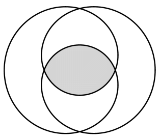
Figure 2. The region $q_{\circ}(\mathbb{D})$ and its preimage for $q=z^{3}+\frac{1}{2}z$

Remark 2.3.

Note that the region $q_{\circ}(D)$ need not be connected in general. To construct an example in which it is not, consider a conformal map $\varphi\colon\mathbb{D}\to\Omega$ from the unit disc onto an annular sector

$$\Omega=\biggl{\{}z\in\mathbb{C}\>\biggl{|}\>\frac{1}{2}<|z|<1,\ 0<{\rm arg}(z)<\frac{3\pi}{2}\biggr{\}}.$$

Such a map $\varphi$ exists by the Riemann mapping theorem and, by Caratheodory’s theorem [Ca13], extends continuously to a map $\Phi\colon\overline{\mathbb{D}}\to\overline{\Omega}$ between the closures. Now $\Phi$ can be approximated uniformly by a sequence of polynomials. Consequently, if $p\in\mathbb{C}[z]$ satisfies

$$\|\Phi-p\|_{\infty,\mathbb{D}}<\varepsilon,$$

the image $p(\mathbb{D})$ has Hausdorff-distance at most $\varepsilon$ from $\Omega$. Put $q=p^{2}$, then, by construction, the complement of the image $q(\mathbb{D})$ is disconnected, the origin being contained in a bounded connected component of $\mathbb{C}\setminus q(\mathbb{D})$. Thus if we consider the circular region $D=\mathbb{C}\setminus\mathbb{D}$, then $q_{\circ}(D)=\mathbb{C}\setminus q(\mathbb{D})$ is not connected.

In order to test whether $q_{\circ}(\mathbb{D})$ is non-empty for a given $q$, we may proceed as follows. Given a monic polynomial $q\in\mathbb{C}[z]_{d}$, write

$$\frac{q^{\#}(x)\overline{q^{\#}(\overline{y})}-q(x)\overline{q(\overline{y})}}{1-xy}=\sum_{j,k=0}^{d-1}a_{jk}x^{j}y^{k}.$$

By the Schur-Cohn criterion (see [KN81, §3.3]), all roots of $q$ are contained in $\mathbb{D}$ if and only if the Hermitian form defined by the $d\times d$-matrix

$${\rm SC}(q)=(a_{jk})_{j,k=0,\dots,d-1}$$

is positive definite. This proves the following.

Proposition 2.4.

The region $q_{\circ}(\mathbb{D})$ is empty if and only if the matrix ${\rm SC}(q-\lambda)$ has a non-positive eigenvalue, for every $\lambda\in\mathbb{C}$.∎

Similar criteria exist for the case of a halfplane instead of a disk.

Example 2.5.

Consider the family of cubic polynomials $q(z)=z^{3}+\gamma z$ for $\gamma\in\mathbb{C}$. We compute the Schur-Cohn matrix and find

$${\rm SC}(q-\lambda)=\begin{bmatrix}1-|\lambda|^{2}&\overline{\lambda}\gamma&\overline{\gamma}\\ \lambda\overline{\gamma}&1-|\lambda|^{2}-|\gamma|^{2}&\overline{\lambda}\gamma\\ \gamma&\lambda\overline{\gamma}&1-|\lambda|^{2}\end{bmatrix}.$$

Thus we see that if $|\gamma|\geqslant 1$, the matrix ${\rm SC}(q-\lambda)$ is not positive definite for any $\lambda$, so that $q_{\circ}(\mathbb{D})=\emptyset$. Conversely, if $|\gamma|<1$, then ${\rm SC}(q)$ is positive definite and hence $q_{\circ}(\mathbb{D})\neq\emptyset$.

For real $\gamma\in(0,1)$, the picture in the complex plane will essentially look the same as in the case $\gamma=\frac{1}{2}$ in Example 2.2 above. For $\gamma=1$, the image curve will degenerate as in Figure 3 and the region $q_{\circ}(\mathbb{D})$ will be empty.

Figure 3. For $q=z^{3}+z$, the region $q_{\circ}(\mathbb{D})$ is empty.

Remark 2.6.

If $q$ is viewed as a rational function on the Riemann sphere $\overline{\mathbb{C}}$, then $q^{-1}(\infty)=\infty$. It follows that if $D$ is an unbounded domain, so that $\infty$ is contained in the closure of $D$ inside $\overline{\mathbb{C}}$, then $\infty$ is also in the closure of $q_{\circ}(D)$, by continuity. In particular, $q_{\circ}(D)$ is non-empty.
More generally, we may consider

$$q_{(k)}(D)=\bigl{\{}u\in\mathbb{C}\>|\>\#(q^{-1}(u)\cap D)=k\bigr{\}},$$

where $\#(q^{-1}(u)\cap D)$ is the cardinality of the fiber, counted with multiplicities. Clearly, the regions $q_{(k)}(D)$ are pairwise disjoint for different values of $k$ and the boundary of $q_{(k)}(D)$ is contained in the curve $q(\partial D)$. Furthermore, we have

$$q_{(d)}(D)=q_{\circ}(D),\quad\bigcup_{k=0}^{d}q_{(k)}(D)=\mathbb{C}\quad\text{and}\quad\bigcup_{k=1}^{d}q_{(k)}(D)=q(D).$$

The regions $q_{(k)}(D)$ can also be characterized in terms of a fiber-counting integral. For example, let $D=\mathbb{C}\setminus\mathbb{D}$ be the complement of the unit disk. For $u\in\mathbb{C}$, let

$$N(u)=\frac{1}{2\pi i}\lim_{R\to\infty}\biggl{(}\int_{|z|=R}\frac{q^{\prime}(z)}{q(z)-u}dz-\int_{|z|=1}\frac{q^{\prime}(z)}{q(z)-u}dz\biggr{)}.$$

Then $N(u)$ is the number of preimages of $u$ under $q$ contained in $D$, counted with multiplicities, so that $q_{(k)}(D)=\{u\in\mathbb{C}\>|\>N(u)=k\}$.

For our purposes, it would be best if we could have $q_{\circ}(D)=q(D)$. Unfortunately, this case does not occur in a non-trivial way, as the following theorem shows.

Theorem 2.7.

The equality $q_{\circ}(\mathbb{D})=q(\mathbb{D})$ occurs if and only if $q=z^{d}+c$ for some $d\geqslant 1$ and $c\in\mathbb{C}$.

Proof.

Let $q\in\mathbb{C}[z]$ be monic of degree $d$ and assume $q_{\circ}(\mathbb{D})=q(\mathbb{D})$, which is equivalent to $q^{-1}(q(\mathbb{D}))=\mathbb{D}$. Write $\mathbb{T}=\partial\mathbb{D}$, then $q^{-1}(q(\mathbb{T}))=\mathbb{T}$ by continuuity. We show first that this implies $q(\mathbb{T})=\partial q(\mathbb{D})$. Note that $q$ is non-constant and hence $q\colon\mathbb{C}\to\mathbb{C}$ is a surjective open map, which implies $\partial q(\mathbb{D})\subset q(\mathbb{T})$. Suppose this inclusion is strict, which means that $q(\mathbb{T})$ contains interior points of $\overline{q(\mathbb{D})}$. Since $q(\mathbb{T})$ is a closed curve, it follows that $\overline{q(\mathbb{D})}\setminus q(\mathbb{T})$ is disconnected. On the other hand, $q^{-1}(q(\mathbb{T}))=\mathbb{T}$ implies $q(\mathbb{D})\cap q(\mathbb{T})=\emptyset$, hence $q(\mathbb{D})$ is disconnected, a contradiction.

From this we see that $q(\mathbb{D})$ is an open subset of $\mathbb{C}$ with connected boundary and hence it is simply connected. Fix a point $a\in q(\mathbb{D})$. By the Riemann mapping theorem, there exists a biholomorphic map $\varphi\colon q(\mathbb{D})\to\mathbb{D}$ with $\varphi(a)=0$. Let $B=\varphi\circ q\colon\mathbb{D}\to\mathbb{D}$. Since $q(\mathbb{D})$ is simply connected and bounded by the Jordan curve $q(\mathbb{T})$, the holomorphic map $B$ extends continuously to a map $\overline{\mathbb{D}}\to\overline{\mathbb{D}}$, by Carathéodory’s theorem [Ca13]. This implies that $B$ has a representation as a finite Blaschke product of degree $d$, i.e. there exists a monic polynomial $h\in\mathbb{C}[z]$ of degree $d$ and $\alpha\in\mathbb{C}$ such that

$$B(z)=\alpha\cdot\frac{h(z)}{h^{\#}(z)}$$

for all $z\in\overline{\mathbb{D}}$ (see for example [Co95, §20]). Let $c_{1},\dots,c_{d}\in\mathbb{C}$ be the zeros of $h$, then $B(c_{k})=\varphi(q(c_{k}))=0$ implies that $c_{1},\dots,c_{d}$ are also zeros of $q(z)-a$, so that $q-a=h$. Factoring $\varphi$ as $\varphi(z)=(z-a)\psi(z)$ for some holomorphic map $\psi\colon q(\mathbb{D})\to\mathbb{C}$, we can write

$$\alpha\cdot\frac{q(z)-a}{q^{\#}(z)-\overline{a}z^{d}}=\alpha\cdot\frac{h(z)}{h^{\#}(z)}=B(z)=\bigl{(}q(z)-a\bigr{)}\psi\bigl{(}q(z)\bigr{)}$$

for $z\in\mathbb{D}$. Dividing both sides by $q(z)-a$ shows

$$q^{\#}(z)-\overline{a}z^{d}=\frac{\alpha}{\psi(q(z))}.$$

Therefore, $q^{\#}(z)-\overline{a}z^{d}$ is a polynomial of degree at most $d$ that is constant along the fibers of $q$. By Lemma 2.8 below, this implies that there exist constants $b,c\in\mathbb{C}$ such that $q^{\#}(z)-\overline{a}z^{d}=bq+c$. But the point $a\in q(\mathbb{D})$ can be chosen arbitrarily, so we obtain constants $b_{a},c_{a}\in\mathbb{C}$ depending on $a\in q(\mathbb{D})$ and identities

$$q^{\#}(z)-\overline{a}z^{d}=b_{a}q+c_{a}.$$

Expanding $q(z)=z^{d}+\sum_{j=0}^{d-1}\alpha_{j}z^{j}$ and comparing leading coefficients on both sides leads to $b_{a}=\overline{\alpha_{0}}-\overline{a}$. After cancelling leading coefficients, we are then left with

$$1+\sum_{j=1}^{d-1}\overline{\alpha_{d-j}}z^{j}=(\overline{\alpha_{0}}-\overline{a})\sum_{j=0}^{d-1}\alpha_{j}z^{j}+c_{a}.$$

For this to hold for all $a\in q(\mathbb{D})$, we must have $\alpha_{1}=\cdots=\alpha_{d-1}=0$, so that $q(z)-z^{d}$ is constant, as claimed. ∎

Lemma 2.8.

If $q,r\in\mathbb{C}[z]$ are two polynomials of the same degree such that $r$ is constant along the fibers of $q$, i.e. $q(z)=q(w)$ implies $r(z)=r(w)$ for all $z,w\in\mathbb{C}$, then there are constants $b,c\in\mathbb{C}$ such that $r=bq+c$.

Proof.

If $q,r$ are constant, there is nothing to show. Otherwise, consider the algebraic curve $Z=\{(z,w)\in\mathbb{C}^{2}\>|\>q(z)=q(w)\}\subset\mathbb{C}^{2}$. By hypothesis, the polynomial $r(z)-r(w)\in\mathbb{C}[z,w]$ vanishes identically on $Z$. Since $q(z)-q(w)$ is square-free, Hilbert’s Nullstellensatz gives an identity

$$r(z)-r(w)=s(z,w)\bigl{(}q(z)-q(w)\bigr{)}$$

for some $s\in\mathbb{C}[z,w]$. Let $\zeta\in\mathbb{C}$ be any zero of $r$, then $r(z)=s(z,\zeta)\bigl{(}q(z)-q(\zeta)\bigr{)}$. Since $r$ and $q$ are of the same degree, $s(z,\zeta)$ must have degree $0$ in $z$, so that putting $b=s(1,\zeta)$ and $c=-s(1,\zeta)q(\zeta)$ yields the desired identity. ∎

3. Symmetrization and pullback

Let $f\in\mathbb{C}[z]_{n}$, $q\in\mathbb{C}[z]_{d}$, with $q$ monic, and consider $\operatorname{Sym}_{nd}(f\circ q)(y_{11},\dots,y_{nd})$, the symmetrization of $f\circ q$ in the $nd$ variables $(y_{jk}\>|\>j=1,\dots,n,k=1,\dots,d)$. Let

$$Q\colon\left\{\begin{array}[]{ccc}\mathbb{C}^{n}&\to&\mathbb{C}^{n}\\ (z_{1},\dots,z_{n})&\mapsto&\bigl{(}q(z_{1}),\dots,q(z_{n})\bigr{)}\end{array}\right..$$

Since $q$ has degree $d$, the fibers of $Q$ can be identified with points in $\mathbb{C}^{nd}$. Let $(u_{1},\dots,u_{n})\in\mathbb{C}^{n}$ and put

$$\bigl{(}y_{11},\dots,y_{nd}\bigr{)}=Q^{-1}(u_{1},\dots,u_{n}).$$

In other words, $y_{j1},\dots,y_{jd}$ are the zeros of the polynomial $q(z)-u_{j}$. We compute the restriction of $\operatorname{Sym}_{nd}(f\circ q)$ to this fiber. By 1.3(5), we have

$$\operatorname{Sym}_{nd}(f\circ q)(y_{11},\dots,y_{nd})=\bigl{\langle}f\circ q,\prod\nolimits_{j=1}^{n}\prod\nolimits_{k=1}^{d}(1+\overline{y_{jk}}z)\bigl{\rangle}_{nd}.$$

Since $q(z)-u_{j}=\prod_{k=1}^{d}(z-y_{jk})$, we find $\prod_{k=1}^{d}(1+\overline{y_{jk}}z)=(q(z)-u_{j})^{\#\vee}$ by 1.2, hence

$$\operatorname{Sym}_{nd}(f\circ q)|_{Q^{-1}(u_{1},\dots,u_{n})}=\bigl{\langle}f\circ q,\prod\nolimits_{j=1}^{n}(q-u_{j})^{\#\vee}\bigl{\rangle}_{nd}.$$

We introduce the following notation.

$$S_{q,n}(f)(u_{1},\dots,u_{n})=\bigl{\langle}f\circ q,\prod\nolimits_{j=1}^{n}(q-u_{j})^{\#\vee}\bigl{\rangle}_{nd}$$

$$T_{q,n}(f)=S_{q,n}(f)(z,\dots,z)$$

Proposition 3.1.

1. $S_{q,n}(f)=\operatorname{Sym}_{n}(T_{q,n}(f))$ for all $f\in\mathbb{C}[z]_{n}$.

2. $\deg\bigl{(}T_{q,n}(f)\bigr{)}=\deg(f)$ for all $f\in\mathbb{C}[z]_{n}$.

3. The leading coefficient of $T_{q,n}(z^{k})$ is

   $$(-1)^{k(d+1)}\textstyle\binom{n}{k}\bigl{/}\binom{nd}{kd}.$$

   These leading coefficients are exactly the eigenvalues of $T_{q,n}$.

4. The linear operator $T_{q,n}\colon\mathbb{C}[z]_{n}\to\mathbb{C}[z]_{n}$ is invertible.

Proof.

(a) By construction, $S_{q,n}(f)$ is symmetric and multiaffine of degree $n$ in $u_{1},\dots,u_{n}$ and satisfies $S_{q,n}(f)(z,\dots,z)=T_{q,n}(f)$. By the uniqueness of the symmetrization, it therefore coincides with $\operatorname{Sym}_{n}(T_{q,n}(f))$.

(b) and (c) For $k\in\{0,\dots,n\}$, we compute

$$S_{q,n}(z^{k})(u,\dots,u)=\langle q^{k},\bigl{(}(q-u)^{\#\vee}\bigr{)}^{n}\rangle_{nd}.$$

If $q(z)=\sum_{j=0}^{d}b_{j}z^{j}$ (where $b_{d}=1$), then

$$(q-u)^{\#\vee}=(-1)^{d}\overline{(b_{0}-u)}z^{d}+\sum\nolimits_{j=1}^{d}(-1)^{d-j}\overline{b_{j}}z^{d-j}.$$

Since monomials in $z$ of different degree are orthogonal and every term of $q^{k}$ has degree at most $kd$ in $z$, we see that $S_{q,n}(z^{k})(u,\dots,u)$ is a polynomial of degree at most $k$ in $u$. Since $T_{q,n}(z^{k})=S_{q,n}(z^{k})(z,\dots,z)$, it follows that $T_{q,n}(z^{k})$ has degree at most $k$ in $z$.

To find the leading coefficient, isolate all terms of degree $k$ in $\overline{u}$ on the right-hand side of the inner product above: These are of the form $\binom{n}{k}(-1)^{k(d+1)}\overline{u}^{k}z^{kd}(zr(z)+1)$ for some polynomial $r\in\mathbb{C}[z]$. Since the left-hand side is of degree $kd$ in $z$ with leading term $z^{kd}$, we have $\langle q^{k},z^{kd}zr(z)\rangle_{nd}=0$. Thus the coefficient of $u^{k}$ is found to be equal to $\binom{n}{k}(-1)^{k(d+1)}\langle z^{kd},z^{kd}\rangle_{nd}=(-1)^{k(d+1)}\binom{n}{k}\bigl{/}\binom{nd}{kd}$, as claimed.

The equality $\deg(T_{q,n}(f))=\deg(f)$ is equivalent to the fact that the matrix representing $T_{q,n}$ in the basis $(1,z,\dots,z^{n})$ is upper-triangular. Its diagonal entries and thus its eigenvalues are exactly the leading coefficients of $T_{q,n}(z^{k})$.

(d) follows from (c). ∎

We say that two polynomials $f,g\in\mathbb{C}[z]_{n}$ are $q$-apolar if

$$[f\circ q,g\circ q]_{nd}=0.$$

The notion of $q$-apolarity is strongly related to the operator $T_{q,n}$, as the following proposition shows.

Proposition 3.2.

We have

$$[f\circ q,g\circ q]_{nd}=[T_{q,n}(f),g]_{n}$$

for all $f,g\in\mathbb{C}[z]_{n}$.

Proof.

If $\deg(g)=n$, let $g=\beta\prod_{j=1}^{n}(z-\mu_{j})$. Using Prop. 3.1(a) and 1.3, we find

$$[f\circ q,g\circ q]_{nd} =\beta\langle f\circ q,\prod\nolimits_{j=1}^{n}(q-\mu_{j})^{\#\vee}\rangle_{nd}=\beta S_{q,n}(f)(\mu_{1},\dots,\mu_{n})$$

$$=\beta\operatorname{Sym}_{n}(T_{q,n}(f))(\mu_{1},\dots,\mu_{n})=[T_{q,n}(f),g]_{n}.$$

If $\deg(g)<n$, the identity also holds, by continuity. ∎

Example 3.3.

Let

$$q(z) =z^{2}+\beta z+\gamma$$

$$f(z) =az^{2}+bz+c$$

Following the above computation, we find

$$S_{q,2}(f)(u_{1},u_{2}) =au_{1}u_{2}+\frac{1}{6}\biggl{(}(2a\Delta-b)(u_{1}+u_{2})+a\Delta^{2}-2b\Delta\biggr{)}+c,$$

where $\Delta=\beta^{2}-4\gamma$ is the discriminant of $q$. Hence

$$T_{q,2}(f)(z)=az^{2}+\frac{1}{6}\biggl{(}(4a\Delta-2b)z+a\Delta^{2}-2b\Delta\biggr{)}+c.$$

With respect to the basis $(1,z,z^{2})$, the operator $T_{q,2}$ is therefore represented by the uppper-triangular matrix

$$\begin{bmatrix}1&-\frac{1}{3}\Delta&\frac{1}{6}\Delta^{2}\\ 0&-\frac{1}{3}&\frac{2}{3}\Delta\\ 0&0&1\end{bmatrix}$$

For a general cubic polynomial

$$f(z)=az^{3}+bz^{2}+cz+d,$$

direct computation shows

$$T_{q,3}(f)(z)=-az^{3}+\frac{1}{10}\bigl{(}2b-9a\Delta\bigr{)}z^{2}+\frac{1}{10}\bigl{(}-3a\Delta^{2}+2b\Delta-2c\bigr{)}z+\frac{1}{20}\bigl{(}-a\Delta^{3}+2b\Delta^{2}-6c\Delta\bigr{)}+d.$$

With respect to the basis $(1,z,z^{2},z^{3})$, the operator $T_{q,3}$ is therefore represented by the upper-triangular matrix

$$\begin{bmatrix}1&-\frac{3}{10}\Delta&\frac{1}{10}\Delta^{2}&-\frac{1}{20}\Delta^{3}\\ 0&-\frac{1}{5}&\frac{1}{5}\Delta&-\frac{3}{10}\Delta^{2}\\ 0&0&\frac{1}{5}&-\frac{9}{10}\Delta\\ 0&0&0&-1\end{bmatrix}$$

Example 3.4.

Let

$$q(z)=z^{3}+\beta z^{2}+\gamma z+\delta\\$$

In the basis $(1,z,z^{2})$ the operator $T_{q,2}\colon\mathbb{C}[z]_{2}\to\mathbb{C}[z]_{2}$ is represented by the matrix

$$\begin{bmatrix}1&\frac{1}{30}\Gamma&-\frac{1}{15}\Delta\\ 0&\frac{1}{10}&-\frac{1}{15}\Gamma\\ 0&0&1\end{bmatrix}$$

where $\Delta=\beta^{2}\gamma^{2}-4\gamma^{3}-4\beta^{3}\delta+18\beta\gamma\delta-27\delta^{2}$ is the discriminant of $q$ and $\Gamma=2\beta^{3}-9\beta\gamma+27\delta$.

The operator $T_{q,3}$ in the basis $(1,z,z^{2},z^{3})$ is represented by the matrix

$$\begin{bmatrix}1&\frac{1}{28}\Gamma&-\frac{1}{28}\Delta&0\\ 0&\frac{1}{28}&0&-\frac{3}{28}\Delta\\ 0&0&\frac{1}{28}&-\frac{3}{28}\Gamma\\ 0&0&0&1\end{bmatrix}$$

We are now ready for the generalized versions of the theorems of Grace and Walsh.

Theorem 3.5 (Generalized Grace theorem).

Let $D$ be a circular domain and $q\in\mathbb{C}[z]$ a monic polynomial of degree $d$. If $f,g\in\mathbb{C}[z]$ are $q$-apolar polynomials of the same degree and all zeros of $f$ lie in $q_{\circ}(D)$, then $g$ has at least one zero in $q(D)$.

Proof.

If $y_{11},\dots,y_{nd}$ are the zeros of $g\circ q$, then $[f\circ q,g\circ q]_{nd}=\operatorname{Sym}_{nd}(f\circ q)(y_{11},\dots,y_{nd})$ by 1.4. So if $[f\circ q,g\circ q]_{nd}=0$, then $(y_{11},\dots,y_{nd})$ is a zero of $\operatorname{Sym}_{nd}(f\circ q)$. Since all zeros of $f$ are in $q_{\circ}(D)$, all zeros of $f\circ q$ are in $D$, and therefore $y_{jk}\in D$ for some $j,k$ by Walsh’s theorem (Thm. 1.5). Hence $q(y_{jk})\in q(D)$ is a zero of $g$. ∎

Theorem 3.6 (Generalized Walsh theorem).

Let $D$ be a circular domain and $q\in\mathbb{C}[z]$ a monic polynomial. Let $f\in\mathbb{C}[z]$ be a polynomial of degree $n$.

1. Assume that all zeros of $f$ lie in $q_{\circ}(D)$. Then all zeros of $T_{q,n}(f)$ lie in $q(D)$ and if $(u_{1},\dots,u_{n})\in\mathbb{C}^{n}$ is a zero of $S_{q,n}(f)=\operatorname{Sym}_{n}(T_{q,n}(f))$, then $u_{k}\in q(D)$ for some $k$.

2. Assume that $f$ does not vanish in $q(D)$. Then $T_{q,n}(f)$ does not vanish in $q_{\circ}(D)$ and $S_{q,n}(f)$ does not vanish in $(q_{\circ}(D))^{n}$.

Proof.

(1) Assume that $S_{q,n}(u_{1},\dots,u_{n})=0$. By definition, $S_{q,n}(f)$ is the restriction of $\operatorname{Sym}_{nd}(f\circ q)$ to the fibers of $q$, so $\operatorname{Sym}_{nd}(f\circ q)(y_{11},\dots,y_{nd})=0$, where $\{y_{j1},\dots,y_{jd}\}=q^{-1}(u_{j})$ for $j=1,\dots,n$. Since all zeros of $f$ are in $q_{\circ}(D)$, the zeros of $f\circ q$ are in $D$. By Walsh’s theorem (Thm. 1.5), this implies $y_{jk}\in D$ for some $j,k$ and hence $u_{j}=q(y_{jk})\in q(D)$, as claimed.

(2) Apply (1) to the circular domain $\mathbb{C}\setminus D$ and use the identities $q(\mathbb{C}\setminus D)=\mathbb{C}\setminus q_{\circ}(D)$ and $q_{\circ}(\mathbb{C}\setminus D)=\mathbb{C}\setminus q(D)$. ∎

Corollary 3.7.

Let $f,g\in\mathbb{C}[z]$ be monic of degree $n$ without common zeros in $q(D)$.

1. Given $y=(y_{1},\dots,y_{n})\in q_{\circ}(D)$ with $S_{q,n}(g)(y)\neq 0$, there exists $z\in q(D)$ with $g(z)\neq 0$ such that

   $$\frac{S_{q,n}(f)(y)}{S_{q,n}(g)(y)}=\frac{f(z)}{g(z)}.$$

2. If $|f/g|\geqslant 1$ on $q(D)$, then

   $$\biggl{|}\frac{S_{q,n}(f)}{S_{q,n}(g)}\biggr{|}\geqslant 1\quad\text{on }\bigl{(}q_{\circ}(D)\bigr{)}^{n}.$$

Proof.

(1) Suppose that $\alpha\in\mathbb{C}$ is not in $(f/g)(q(D))$. Since $f$ and $g$ have no common zeros in $q(D)$, this implies that $f-\alpha g$ does not vanish anywhere in $q(D)$. Then $S_{q,n}(f-\alpha g)=S_{q,n}(f)-\alpha S_{q,n}(g)$ does not vanish anywhere in $(q_{\circ}(D))^{n}$ by Thm. 3.6(2), so $\alpha$ is not assumed by the rational function $S_{q,n}(f)/S_{q,n}(g)$ on $(q_{\circ}(D))^{n}$. (2) follows immediately from (1). ∎

Example 3.8.

Let $q(z)=z^{3}+\gamma z$ where $\gamma$ is real and positive (c.f. Example 2.2). The region $q_{\circ}(\mathbb{D})$ contains the disc $B_{0}(1+\gamma)$, while $q(D)$ is contained in the disc $B_{0}(1-\gamma)$. Now a weaker version of Cor. 3.7 says that given $f,g\in\mathbb{C}[z]_{n}$ such that $|(f/g)(z)|\geqslant 1$ for all $z$ with $|z|>1-\gamma$, we must have $|(S_{q,n}(f)/S_{q,n}(g))(y_{1},\dots,y_{n})|$ for all $y_{1},\dots,y_{n}$ with $|y_{k}|>1+\gamma$ for $k=1,\dots,n$.
For instance, if $a,b,c,d\in\mathbb{C}$ are such that

$$|az^{3}+bz^{2}+cz+d|\geqslant 1\quad\text{whenever}\quad|z|>1-\gamma$$

it follows that

$$\bigl{|}\bigl{(}1+\gamma^{3}/7\bigr{)}ay_{1}y_{2}y_{3}+\bigl{(}1/84+\gamma^{3}/7\bigr{)}b(y_{1}y_{2}+y_{1}y_{3}+y_{2}y_{3})+1/84c(y_{1}+y_{2}+y_{3})+d\bigr{|}\geqslant 1$$

whenever $|y_{1}|,|y_{2}|,|y_{3}|>1+\gamma$.

4. Skew eigenfunctions

Let $\mathcal{H}$ be a complex Hilbert space. Recall that a map $\Phi\colon\mathcal{H}\to\mathcal{H}$ is called antilinear if $\Phi(x+y)=\Phi(x)+\Phi(y)$ and $\Phi(\alpha x)=\overline{\alpha}\Phi(x)$ hold for all $x,y\in\mathcal{H}$, $\alpha\in\mathbb{C}$. If $\langle\Phi x,\Phi y\rangle=\langle y,x\rangle$ holds for all $x,y\in\mathcal{H}$, then $\Phi$ is called isometric.

Definition 4.1.

Let $\mathcal{H}$ be a complex Hilbert space. A map $C\colon\mathcal{H}\to\mathcal{H}$ is called an antilinear conjugation if it is antilinear, isometric and satisfies

$$C^{2}=\varepsilon\cdot{\rm id},\text{ where }\varepsilon\in\{-1,1\}.$$

Lemma 4.2.

Let $\mathcal{H}$ be a complex Hilbert space of finite dimension $n$ and let $J\colon\mathcal{H}\to\mathcal{H}$ be an antilinear isometry with $J^{2}=\operatorname{id}$. Then there exists an orthonormal basis $f_{1},\dots,f_{n}$ such that $Jf_{k}=f_{k}$ for $k=1,\dots,n$.

Proof.

Take any vector $h\in\mathcal{H}$ with $||h||=1$. Then $g=(h+Jh)/2$ satisfies $Jg=g$. If $g\neq 0$, we put $f_{1}=g$. If $g=0$, this means $Jh=-h$. We put $f_{1}=ih$, so that $Jf_{1}=Jih=-iJh=ih=f_{1}$. Now since $J$ is an isometry, the orthogonal complement $h_{1}^{\perp}$ is $J$-invariant and the claim follows by induction. ∎

Theorem 4.3.

Let $\mathcal{H}$ be a complex Hilbert space of finite dimension $n$ equipped with an antilinear conjugation $C$. Let $T\colon\mathcal{H}\to\mathcal{H}$ be an invertible linear map satisfying

$$T^{\ast}=CTC.$$

1. There exists an antilinear conjugation $J$ with $J^{2}={\rm id}$ that commutes with $|T|$, where $|T|=\sqrt{T^{\ast}T}$, and satisfies $T=CJ|T|$.

2. There exists an orthonormal basis $f_{1},\dots,f_{n}$ of $\mathcal{H}$ such that

   $$Tf_{k}=\lambda_{k}Cf_{k}\quad\text{for }k=1,\dots,n,$$

   where $\lambda_{1},\dots,\lambda_{n}\in\mathbb{R}_{+}$ are the singular values of $T$.

Proof.

(1) Write $C^{2}=\varepsilon\cdot{\rm id}$ as above and let $T=U|T|$ be the polar decomposition of $T$, where $U$ is unitary. Then $T^{\ast}=|T|U^{\ast}$ and $T=CT^{\ast}C=(CU^{\ast}C)(\varepsilon CU|T|U^{\ast}C)$. Put $U^{\prime}=CU^{\ast}C$ and $P=\varepsilon CU|T|U^{\ast}C$. Since $C$ and $U$ are both unitary, so is $U^{\prime}$. Furthermore, since $|T|$ is positive definite, we have

$$\langle Px,x\rangle=\langle\varepsilon CU|T|U^{\ast}Cx,x\rangle=\langle CU|T|U^{\ast}Cx,C^{2}x\rangle=\langle Cx,U|T|U^{\ast}Cx\rangle>0$$

for any $x\neq 0$ in $\mathcal{H}$, which shows that $P$ is also positive definite. By the uniqueness of the polar decomposition, $T=U|T|=U^{\prime}P$ implies $U=U^{\prime}$ and $|T|=P$. The first equality means $U=CU^{\ast}C$, hence $\varepsilon CU=U^{\ast}C$. Put $J=U^{\ast}C$, then $J^{2}=\varepsilon CUU^{\ast}C={\rm id}$. Also, $J$ is antilinear and $\langle Jx,Jy\rangle=\langle U^{\ast}Cx,U^{\ast}Cy\rangle=\langle Cx,Cy\rangle=\langle y,x\rangle$, hence $J$ is isometric. Thus $J$ is an antilinear conjugation. It also commutes with $|T|$, since $J|T|J=\varepsilon CU|T|U^{\ast}C=P=|T|$.

(2) Let $\lambda_{1},\dots,\lambda_{n}$ be the singular values of $T$, i.e. the eigenvalues of $|T|$. Applying Lemma 4.2 for the restriction of $J$ to each eigenspace of $|T|$, we choose an orthonormal basis $f_{1},\dots,f_{n}$ of corresponding eigenvectors of $|T|$ each of which is fixed under $J$. We then have

$$Tf_{k}=CJ|T|f_{k}=C|T|f_{k}=\lambda_{k}Cf_{k}$$

for $k=1,\dots,n$, as desired. ∎

We apply the above result in the case $\mathcal{H}=\mathbb{C}[z]_{n}$ and obtain the following statement.

Corollary 4.4.

If $q\in\mathbb{C}[z]$ is monic and of even degree, there exists a basis $f_{0},\dots,f_{n}$ of $\mathbb{C}[z]_{n}$ which is orthonormal with respect to the Fischer inner product and satisfies

$$[f_{j}\circ q,f_{k}\circ q]_{nd}=\lambda_{j}\delta_{jk},$$

for all $j,k=0,\dots,n$, where $\lambda_{0},\dots,\lambda_{n}$ are the singular values of the operator $T_{q,n}$.

In other words, the base-polynomials furnished by Thm. 4.3 are both orthonormal and pairwise $q$-apolar.

Proof.

Let $d=\deg(q)$ and put

$$C\colon\mathbb{C}[z]_{n}\to\mathbb{C}[z]_{n},\ p\mapsto p^{\#\vee}.$$

and $T=T_{q,n}$. It is easily checked that $C$ is indeed an antilinear conjugation with $\varepsilon=(-1)^{n}$. The identity $T^{\ast}=CTC$ in the hypothesis of Thm. 4.3 then follows from Prop. 3.2: For all $f,g\in\mathbb{C}[z]_{n}$, we have

$$\langle Tf,g\rangle_{n} =[Tf,\varepsilon Cg]_{n}=[f\circ q,(\varepsilon Cg)\circ q]_{nd}$$

$$=[(\varepsilon Cg)\circ q,f\circ q]_{nd}=[T(\varepsilon Cg),f]_{n}=\varepsilon[f,T(\varepsilon Cg)]_{n}=$$

$$=\langle f,CTCg\rangle_{n},$$

hence $T^{\ast}=CTC$, as claimed. (Note that $[-,-]_{nd}$ is symmetric, since $d$ is even.)

Now the $f_{0},\dots,f_{n}$ of $\mathbb{C}[z]_{n}$ given by Thm. 4.3(2) indeed satisfy

$$[f_{j}\circ q,f_{k}\circ q]_{n} =[Tf_{j},f_{k}]_{n}=\langle Tf_{j},Cf_{k}\rangle_{n}$$

$$=\langle\lambda_{j}Cf_{j},Cf_{k}\rangle_{n}=\lambda_{j}\delta_{jk}$$

by Prop. 3.2, since $C$ is isometric. ∎