Double Well Potential Function and Its Optimization in The n-dimensional Real Space – Part I

Abstract

A special type of multi-variate polynomial of degree 4, called the double well potential function, is studied. When the function is bounded from below, it has a very unique property that two or more local minimum solutions are separated by one local maximum solution, or one saddle point. Our intension in this paper is to categorize all possible configurations of the double well potential functions mathematically. In part I, we begin the study with deriving the double well potential function from a numerical estimation of the generalized Ginzburg-Landau functional. Then, we solve the global minimum solution from the dual side by introducing a geometrically nonlinear measure which is a type of Cauchy-Green strain. We show that the dual of the dual problem is a linearly constrained convex minimization problem, which is mapped equivalently to a portion of the original double well problem subject to additional linear constraints. Numerical examples are provided to illustrate the important features of the problem and the mapping in between.

Key Words: Non-convex quadratic programming, Polynomial optimization, Generalized Ginzburg-Landau functional, Double well potential, Canonical duality.

1 Introduction

In this paper, we propose a model that minimizes a special type of multi-variate polynomial of degree 4 in the following form:

$$(\mathrm{DWP}):\ \ \ \min\left\{\frac{1}{2}\left(\frac{1}{2}\|Bx-c\|^{2}-d\right)^{2}+\frac{1}{2}x^{T}Ax-f^{T}x\;|\;\;x\in R^{n}\right\},$$ (1)

where $A$ is an $n\times n$ real symmetric matrix, $B\not=0$ is an $m\times n$ real matrix, $c\in R^{m}$, $d\in R$, and $f\in R^{n}$. Typical examples with properly selected parameters of the objective function are shown in Figure 1. The left most picture in Figure 1 is the simplest example with $n=1$ where there are two local energy wells separated by one barrier. A higher dimensional analogy is shown in the center picture of Figure 1. Note that the barrier in this case is not a local maximum but a saddle point. The figure in the right most is called the Mexican hat potential. It is created by selecting a negative definite matrix $B$ and setting $A=0,f=0$ and $c=0$. It forms a ring-shaped region of infinitely many global minima with one unique local maximum sitting in the center. Due to the common feature shown in these illustrative examples, the objective function is called a double well potential function and the (DWP) model is referred to as the double well potential problem.

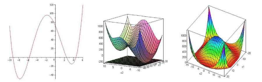
Figure 1: Illustrative examples for the double well potential functions (DWP).

One motivation to investigate the (DWP) problem came from numerical approximations to the generalized Ginzburg-Landau functionals [10]. The functionals often describe the total energy of a ferroelectric system such as the ion-molecule reactions [4]. In a ferromagnetic spin system, the critical phenomena and the phase transition is studied by the mean field approach which also involves a double well potential [3, 14]. Other applications of the Ginzburg-Landau functionals can be found in solid mechanics and quantum mechanics [10, 11].

The mathematical formula of the generalized Ginzburg-Landau functionals takes the following general form [10, 13]:

$$I^{\alpha}(\mu)=\int_{\Omega}[\frac{1}{n}\|\nabla\mu(x)\|^{n}+\frac{\alpha}{2}(\frac{1}{2}\|\mu(x)\|^{2}-\beta)^{2}]dx,$$ (2)

where $\Omega\subset R^{n}$, $\alpha,\beta$ are positive material constants, and $\mu:\Omega\longrightarrow R^{q}$ is a smooth vector-valued (field) function describing the phase (order) of the system. It is known that, when $\alpha$ is sufficiently large (so that the second term dominates), if the trace of $\mu$ on the boundary $\partial\Omega$ is a function of non-zero Brouwer degree, then the generalized Ginzburg-Landau functional $I^{\alpha}(\mu)$ is bounded from below by $\ln\alpha$ [13]. The second term of (2) is actually the double-well potential in the integral form. Directly minimizing $I^{\alpha}(\mu)$ over any reasonable functional space is, in general, very difficult. Hence only the lower bound is estimated in the literature. We therefore look into the discrete version of (2) and it naturally leads to a special case of (1).

To illustrate how (2) can be discretized into (1), we work out an example with $n=2$, $q=1$, and $\Omega=\Omega_{x}\times\Omega_{y}=[0,1]\times[0,1]$. Let $\{0=x_{1}<x_{2}<\ldots<x_{s+1}=1\}$ be a partition of $\Omega_{x}$ that divides $[0,1]$ into $s$ subintervals of equal length. Similarly, let $\{0=y_{1}<y_{2}<\ldots<y_{t+1}=1\}$ be the uniform grid of $\Omega_{y}$. Define an $(s+1)\times(t+1)$ vector $e$ by

$$e=[e_{1,1},e_{2,1},\cdots,e_{s+1,1},e_{1,2},e_{2,2},\cdots,e_{s+1,2},\cdots,e_{1,t+1},e_{2,t+1},\cdots,e_{s+1,t+1}]^{T},$$

where $e_{i,j}=\mu(x_{i},y_{j})$. With the partition, we can approximate $\nabla\mu$ by the first order difference and approximate $I^{\alpha}(\mu)$ by the Riemann sum so that a discrete version of (2) becomes

$$\sum\limits_{i=1}^{s}\sum\limits_{j=1}^{t}\frac{1}{2}|(\frac{e_{i+1,j}-e_{i,j}}{\frac{1}{s}})^{2}+(\frac{e_{i,j+1}-e_{i,j}}{\frac{1}{t}})^{2}|\cdot\frac{1}{s}\frac{1}{t}+\sum\limits_{i=1}^{s}\sum\limits_{j=1}^{t}\frac{\alpha}{2}(\frac{1}{2}e_{i,j}^{2}-\beta)^{2}\cdot\frac{1}{t}\frac{1}{s}$$

$$=\sum\limits_{i=1}^{s}\sum\limits_{j=1}^{t}\frac{s}{2t}(e_{i+1,j}-e_{i,j})^{2}+\sum\limits_{i=1}^{s}\sum\limits_{j=1}^{t}\frac{t}{2s}(e_{i,j+1}-e_{i,j})^{2}+\sum\limits_{i=1}^{s}\sum\limits_{j=1}^{t}\frac{\alpha}{2st}(\frac{1}{2}e_{i,j}^{2}-\beta)^{2}$$

$$\begin{array}[]{ll}=&\displaystyle{\sum\limits_{i=1}^{s}\sum\limits_{j=1}^{t}}\frac{s}{2t}(e_{i,j},e_{i+1,j})E(e_{i,j},e_{i+1,j})^{T}+\sum\limits_{i=1}^{s}\sum\limits_{j=1}^{t}\frac{t}{2s}(e_{i,j},e_{i,j+1})E(e_{i,j},e_{i+1,j})^{T}\\ &+\displaystyle{\sum\limits_{i=1}^{s}\sum\limits_{j=1}^{t}}\frac{\alpha}{2st}(\frac{1}{2}e_{i,j}^{2}-\beta)^{2}\end{array}$$ (5)

where $E=\tiny{\left[\begin{array}[]{cc}1&-1\\ -1&1\end{array}\right]}$. The sum of quadratic forms in (5) can be further combined into a large quadratic form. Let $\mathcal{B}_{i}=Diag(0_{i-1},E,0_{(s+1)(t+1)-i-1})$, where $0_{k}$ is a $k\times k$ block matrix of $0$. Then,

$$\begin{array}[]{l}\sum\limits_{i=1}^{s}\sum\limits_{j=1}^{t}\frac{s}{2t}(e_{i,j},e_{i+1,j})E(e_{i,j},e_{i+1,j})^{T}=\frac{1}{2}e^{T}(\frac{s}{t}\sum\limits_{i\in\mathcal{T}}\mathcal{B}_{i})e\end{array}$$ (7)

where $\mathcal{T}=\{1,2,3,\cdots,(s+1)t\}\backslash\{(s+1),2(s+1),3(s+1),\cdots,t(s+1)\}$. Analogously, we can define $\mathcal{C}_{i}$ to be an $(s+1)(t+1)\times(s+1)(t+1)$ matrix with the $(i,i)$ and $(i+(s+1),i+(s+1))$ components being $1$, $(i,i+(s+1))$ and $(i+(s+1),i)$ components being $-1$, and $0$ elsewhere. Then,

$$\begin{array}[]{l}\sum\limits_{i=1}^{s}\sum\limits_{j=1}^{t}\frac{t}{2s}(e_{i,j},e_{i,j+1})E(e_{i,j},e_{i,j+1})^{T}=\frac{1}{2}e^{T}(\frac{t}{s}\sum\limits_{i\in\mathcal{T}}\mathcal{C}_{i})e.\end{array}$$ (9)

For the third term in (5), we have

$$\begin{array}[]{l}\sum\limits_{i=1}^{s}\sum\limits_{j=1}^{t}\frac{\alpha}{2st}(\frac{1}{2}e_{i,j}^{2}-\beta)^{2}=\frac{\alpha}{8st}\sum\limits_{i=1}^{s}\sum\limits_{j=1}^{t}e_{i,j}^{4}-\frac{\alpha\beta}{2st}\sum\limits_{i=1}^{s}\sum\limits_{j=1}^{t}e_{i,j}^{2}+\frac{\alpha\beta^{2}}{2}.\end{array}$$ (11)

Since

$$\begin{array}[]{l}\sum\limits_{i=1}^{s}\sum\limits_{j=1}^{t}e_{i,j}^{2}=e^{T}e-\sum\limits_{i=1}^{s+1}e_{i,t+1}^{2}-\sum\limits_{j=1}^{t}e_{s+1,j}^{2}\leq\|e\|^{2}\end{array}$$ (13)

and

$$\begin{array}[]{rl}\sum\limits_{i=1}^{s}\sum\limits_{j=1}^{t}e_{i,j}^{4}&=\sum\limits_{i=1}^{s}\sum\limits_{j=1}^{t}(e_{i,j}^{2})^{2}\\ &=(\sum\limits_{i=1}^{s}\sum\limits_{j=1}^{t}e_{i,j}^{2})^{2}-\sum\limits_{(i,j)\neq(k,l)}e_{i,j}^{2}e_{k,l}^{2}\\ &\leq(\sum\limits_{i=1}^{s}\sum\limits_{j=1}^{t}e_{i,j}^{2})^{2}\\ &\leq(\|e\|^{2})^{2},\end{array}$$ (18)

the generalized Ginzburg-Landau functional $I^{\alpha}(u)$ in this example has an estimated upper bound of

$$\begin{array}[]{l}\frac{\alpha}{8ts}(\|e\|^{2})^{2}+\frac{1}{2}e^{T}(\frac{s}{t}\sum\limits_{i\in\mathcal{T}}\mathcal{B}_{i}+\frac{t}{s}\sum\limits_{i\in\mathcal{T}}\mathcal{C}_{i}-\frac{\alpha\beta}{ts}I)e+\frac{\alpha\beta^{2}}{2},\end{array}$$ (20)

which is of the form (1) with $x=e$, $B=(\frac{\alpha}{ts})^{\frac{1}{4}}I$, $A=(\frac{s}{t}\sum\limits_{i\in\mathcal{T}}\mathcal{B}_{i}+\frac{t}{s}\sum\limits_{i\in\mathcal{T}}\mathcal{C}_{i}-\frac{\alpha\beta}{ts}I)$, $c=0$, $d=0$, and $f=0$.

In this paper, we are aimed to categorize all possible configurations and important features of the double well potential functions defined by (1). In part I of the paper, we shall focus on finding the global minimum solution(s), deriving the duality theorem, and analyzing the dual of the dual problem. In part II, we shall study the local (non-global) extremum solution(s) and prove that for the non-singular case, there is at most one local non-global minimum point (namely, at most one local non-global energy well) and at most one local maximum point (at most one energy barrier). Moreover, the radius of the local maximizer is always smaller than that of local/global minimizers, which proves mathematically that the energy barrier (maximizer) is always surrounded by other energy wells (minimizers). Combining the resutls from both Part I and Part II, we conclude that, except for some unbounded cases and singular cases (which can be easily analyzed), the only non-trivial examples of the double well potential function in (1) are those illustrated by Figure 1.

2 Space reduction and format setting

Our approach to solving the global minimum solution of (1) is via the canonical dual transformation, i.e., by introducing geometrically nonlinear measure (Cauchy-Green type strain) $\xi(x):R^{n}\rightarrow R$ defined by

$$\xi=\frac{1}{2}(Bx-c)^{T}(Bx-c)-d.$$

The fourth order polynomial optimization problem (DWP) is then reduced into the following quadratic program with a single quadratic equality constraint, called (QP1QC):

$$\begin{array}[]{rcl}\min&&\Pi(x,\xi)=\frac{1}{2}\xi^{2}+\frac{1}{2}x^{T}Ax-f^{T}x\\ s.t.&&\xi=\frac{1}{2}x^{T}B^{T}Bx-c^{T}Bx+\frac{1}{2}c^{T}c-d\\ &&\ \ x\in R^{n},~{}~{}\xi\in R.\end{array}$$ (24)

Notice that there exists a list of research work on solving (QP1QC). In the rest of this paper, we extend the results of [5, XFGSZ] to study the problem (24) in an explicit manner.

The problem (QP1QC) is a nonconvex optimization problem. It often requires some dual information for providing a global lower bound in order to determine the global minimum solution. Lagrange duality is the most frequently used dual, but it imposes a serious restriction, called the constraint qualification, on the type of nonconvex optimization problems to apply. For other problems not even satisfying any constraint qualification, they are often referred to as the “hard case” in contrast to the easier ones at least with some dual information to help.

In [5], for solving a quadratic program with one quadratic inequality constraint, the (dual) Slater constraint qualification is relaxed to a more general condition called “simultaneously diagonalizable via congruence” (SDC in short). For the (DWP) problem, the (SDC) condition amounts to the two matrices $A$ and $B^{T}B$ are simultaneously diagonalizable via congruence. Namely, there exists a nonsingular matrix $P$ such that both $P^{T}AP$ and $P^{T}B^{T}BP$ become diagonal matrices. Unfortunately, for any given double well potential problem (1), $A$ and $B^{T}B$ may not satisfy (SDC). For example, $A=\tiny{\left[\begin{array}[]{cc}1&-1\\ -1&0\end{array}\right]}$, $B=\tiny{\left[\begin{array}[]{cc}1&-2\\ 3&-6\end{array}\right]}$ is such an instance. In other words, some of the double well potential problem belongs to the “hard case”. Fortunately, we can show in this section that $A$ and $B^{T}B$ of problem (24) can be always made to satisfy the (SDC) condition after performing the following space reduction technique.

Let $U=[u_{1},u_{2},\cdots,u_{r}]$ be a basis for the null space of $B$. First we extend $U$ to a nonsingular $n\times n$ matrix $[U,V]$ such that $BU=0$ and each $x\in R^{n}$ can be split as $x=Uy+Vz$ with $y\in R^{r}$ and $z\in R^{n-r}$. Then, in terms of variables $\xi$, $y$ and $z$, the problem (24) becomes

$$\left\{\begin{array}[]{ll}\displaystyle\min_{\xi,y,z}&\frac{1}{2}\xi^{2}+\frac{1}{2}(y^{T},z^{T})[U,V]^{T}A[U,V](y^{T},z^{T})^{T}-f^{T}[U,V](y^{T},z^{T})^{T}\\ \mbox{s.t.}&\frac{1}{2}(y^{T},z^{T})[U,V]^{T}B^{T}B[U,V](y^{T},z^{T})^{T}-\xi-(B^{T}c)^{T}[U,V](y^{T},z^{T})^{T}-(d-\frac{1}{2}c^{T}c)=0.\end{array}\right.$$ (27)

Equivalently,

$$\left\{\begin{array}[]{ll}\displaystyle\min_{\xi,y,z}&\frac{1}{2}\xi^{2}+\frac{1}{2}y^{T}A_{uu}y+\frac{1}{2}z^{T}A_{vv}z+y^{T}A_{uv}z-f^{T}Uy-f^{T}Vz\\ \mbox{s.t.}&\frac{1}{2}z^{T}B_{vv}z-\xi-(B^{T}c)^{T}Vz-(d-\frac{1}{2}c^{T}c)=0,\end{array}\right.$$ (31)

where $A_{uu}=U^{T}AU,A_{vv}=V^{T}AV,A_{uv}=U^{T}AV=A_{vu}^{T}$, $B_{uu}=U^{T}B^{T}BU$, $B_{vv}=V^{T}B^{T}BV$ and $B_{uv}=U^{T}B^{T}BV=B_{vu}^{T}.$ Notice that the variable splitting ends up with the positive definiteness of matrix $B_{vv}$ and the elimination of variable $y$ in the constraint of (31). As the result, we can solve $y$ first with the variables $\xi$ and $z$ fixed. It amounts to writing (31) as the following two-level optimization problem:

$$\min_{(\xi,z)\in{\cal E}}\{\frac{1}{2}\xi^{2}+\frac{1}{2}z^{T}A_{vv}z-f^{T}Vz+\min\limits_{y\in\mathbb{R}^{r}}\ \{\frac{1}{2}y^{T}A_{uu}y+y^{T}A_{uv}z-f^{T}Uy\}\},$$ (32)

where ${\cal E}=\{(\xi,z)\in R\times R^{n-r}|\frac{1}{2}z^{T}B_{vv}z-\xi-(B^{T}c)^{T}Vz-(d-\frac{1}{2}c^{T}c)=0\}$.

Clearly, if $A_{uu}$ is not positive semi-definite or if $A_{uu}$ is a zero matrix but $A_{uv}z-U^{T}f\neq 0$ for some $(\xi,z)\in\mathcal{E}$, we can immediately conclude that the problems (32) and (DWP) are both unbounded below. When $A_{uu}=0$ and $A_{uv}z-U^{T}f=0,\forall(\xi,z)\in\mathcal{E}$, problem (32) is reduced to

$$\left\{\begin{array}[]{ll}\displaystyle{\min_{\xi,z}}&\frac{1}{2}\xi^{2}+\frac{1}{2}z^{T}A_{vv}z-f^{T}Vz\\ \mbox{s.t.}&\frac{1}{2}z^{T}B_{vv}z-\xi-(B^{T}c)^{T}Vz-(d-\frac{1}{2}c^{T}c)=0,\end{array}\right.$$ (35)

which is the format of (24) with $B_{vv}\succ 0$ on a lower dimensional space.

Suppose $A_{uu}\succeq 0$ with at least one positive eigenvalue, and $(\xi,z)\in\cal{E}$. Then, the optimal solution $y^{*}$ that solves

$$\min_{y\in R^{r}}\ \frac{1}{2}y^{T}A_{uu}y+y^{T}A_{uv}z-f^{T}Uy$$ (36)

must satisfy $A_{uu}y+A_{uv}z-U^{T}f=0$. Assume that $W$ is the null space of $A_{uu}$ and $W$ is of $k$-dimensional. Then, the optimal solution for (36) can be expressed as

$$y^{*}(\beta)=-A_{uu}^{+}U^{T}(AVz-f)+W\beta,\ \forall\beta\in R^{k},$$ (37)

where $A_{uu}^{+}$ is the Moore-Penrose pseudoinverse of $A_{uu}$, and $A_{uu}^{+}=A_{uu}^{-1}$ when $A_{uu}\succ 0$. Then the optimal value of (36) becomes $-\frac{1}{2}(AVz-f)^{T}UA_{uu}^{+}U^{T}(AVz-f).$ Consequently, (32) becomes

$$\left\{\begin{array}[]{ll}\displaystyle{\min_{\xi,z}}&\frac{1}{2}\xi^{2}+\frac{1}{2}z^{T}A_{vv}z-f^{T}Vz-\frac{1}{2}(AVz-f)^{T}UA_{uu}^{+}U^{T}(AVz-f)\\ \mbox{s.t.}&\frac{1}{2}z^{T}B_{vv}z-\xi-(B^{T}c)^{T}Vz-(d-\frac{1}{2}c^{T}c)=0.\end{array}\right.$$ (40)

Simplifying the expressions, we can write (40) as

$$\left\{\begin{array}[]{ll}\displaystyle{\min_{\xi,z}}&\frac{1}{2}\xi^{2}+\frac{1}{2}z^{T}V^{T}\hat{A}Vz-\hat{f}^{T}Vz-\frac{1}{2}f^{T}UA_{uu}^{+}U^{T}f\\ \mbox{s.t.}&\frac{1}{2}z^{T}B_{vv}z-\xi-(B^{T}c)^{T}Vz-(d-\frac{1}{2}c^{T}c)=0,\end{array}\right.$$ (43)

where $\hat{A}=(I-AUA_{uu}^{+}U^{T})A$, $\hat{f}=(I-AUA_{uu}^{+}U^{T})f$, and $B_{vv}\succ 0$. Combining (35) and (43), we may simply assume that $B^{T}B$ is positive definite in (24) throughout the paper.

Performing Cholesky factorization on the positive definite $B^{T}B$ matrix, we have a nonsingular lower-triangular matrix $P_{1}$ such that $P_{1}^{T}(B^{T}B)P_{1}=I$. Since $A$ and $P_{1}^{T}{A}P_{1}$ are symmetric, there is an orthogonal matrix $P_{2}$ such that $P_{2}^{T}P_{1}^{T}{A}P_{1}P_{2}=Diag(\alpha_{1},\alpha_{2},\cdots,\alpha_{n})$ is a diagonal matrix and $P_{2}^{T}P_{1}^{T}(B^{T}B)P_{1}P_{2}=I$. In other words, ${A}$ and $B^{T}B$ satisfies the (SDC) condition if $B^{T}B\succ 0$.

Let $P=P_{1}P_{2}$ and define $w=P^{-1}x,\psi=P^{T}f,\varphi=P^{T}B^{T}c,\nu=d-\frac{1}{2}c^{T}c$. Problem (24) can be written as the sum of separated squares in the following form:

$$\begin{array}[]{lll}(P)~{}~{}~{}P_{0}=&\min&\ \Pi(\xi,w)=\frac{1}{2}\xi^{2}+\sum_{i=1}^{n}(\frac{1}{2}\alpha_{i}w_{i}^{2}-\psi_{i}w_{i})\\ &\mbox{s.t.}&(\xi,w)\in{\cal E}_{a}=\{(\xi,w)\in R\times R^{n}|\;\;\xi=\Lambda(w)\},\end{array}$$ (46)

where $\Lambda(w)=\sum_{i=1}^{n}(\frac{1}{2}w_{i}^{2}-\varphi_{i}w_{i})-\nu$ is the standard geometrically nonlinear (quadratic in this case) operator in the canonical duality theory. We shall call (46) the canonical primal problem $(P)$, since it is the main form that we deal with in this paper.

Let $\sigma\in R$ be the Lagrange multiplier corresponding to the constraint $\xi-\Lambda(w)=0$ in the canonical primal problem (46). The Lagrange function becomes

$$L(\xi,w,\sigma)=\Pi(\xi,w)+\sigma(\Lambda(w)-\xi)=\frac{1}{2}\xi^{2}+\sum\limits_{i=1}^{n}(\frac{1}{2}(\alpha_{i}+\sigma)w_{i}^{2}-(\psi_{i}+\sigma\varphi_{i})w_{i})-\sigma\xi-\sigma\nu.$$

When $\sigma\in{\cal S}_{a}^{+}=(\sigma_{0},+\infty)$ with $\sigma_{0}=\max\{-\alpha_{1},-\alpha_{2},\cdots,-\alpha_{n}\}$, $L(\xi,w,\sigma)$ is convex in $(\xi,w)$. The unique global minimum of $L(\xi,w,\sigma)$, denoted by $(\xi(\sigma),w(\sigma))$, is attained at $w(\sigma)_{i}=\frac{\psi_{i}+\sigma\varphi_{i}}{\alpha_{i}+\sigma}$ and $\xi(\sigma)=\sigma$. The dual problem of (P) is thus formulated as

$$(D)~{}~{}~{}\Pi_{0}^{d}=\sup_{\sigma\in{\cal S}^{+}_{a}}\left\{\Pi^{d}(\sigma)=-\frac{1}{2}\sigma^{2}-\frac{1}{2}\sum_{i=1}^{n}\frac{(\psi_{i}+\sigma\varphi_{i})^{2}}{\alpha_{i}+\sigma}-\nu\sigma\right\}.$$ (47)

It is clear that this canonical dual is a concave maximization problem on a convex feasible space ${\cal S}^{+}_{a}$.

Remark 1

In Gao-Strang [6], $L(\xi,w,\sigma)$ is called the pseudo-Lagrangian associated with the canonical primal problem $(P)$. Since $L(\xi,w,\sigma)$ is convex in $\xi$ for any given $(w,\sigma)$, the total complementary function $\Xi(w,\sigma)$ can be obtained as

$$\Xi(w,\sigma)=\inf_{\xi\in R}L(\xi,w,\sigma)=-\frac{1}{2}\sigma^{2}+\sum_{i=1}^{n}(\frac{1}{2}(\alpha_{i}+\sigma)w_{i}^{2}-(\psi_{i}+\sigma\varphi_{i})w_{i})-\sigma\nu.$$ (48)

By the canonical duality theory [8], the canonical dual function can be defined by

$$\Pi^{d}(\sigma)=\inf\{\Xi(w,\sigma)|\;w\in R^{n}\},$$

which is the same as (47) and is called the total complementary energy.

In finite deformation theory, if the quadratic operator $\Lambda(w)$ represents a Cauchy-Green strain measure and $\alpha_{i}=0\;\forall i\in\{1,\dots,n\}$, the canonical primal function $\Pi(\xi,w)$ is the total potential energy (see Equation (13) in [6]). The total complementary function $\Xi(w,\sigma)$ then leads to the well-known Hellinger-Reissner generalized complementary energy, and the pseudo-Lagrangian is the Hu-Washizu generalized potential energy, proposed independently by Hu Hai-Chang [12] and K. Washizu [17] in 1955 (see Chapter 6.3.3 in [8]). The extremality of these functions and the existence of a total complementary energy $\Pi^{d}(\sigma)$ as the canonical dual to $\Pi(\xi,w)$ have been debated in the community of theoretical and applied mechanics for several decades (see [15]). Gao and Strang [6] revealed the extremality relations among these functions, and the term

$$G_{ap}(w,\sigma)=\sum_{i=1}^{n}\frac{1}{2}(\alpha_{i}+\sigma)w_{i}^{2}$$

is called the complementary gap function. Their general global sufficient condition $G_{ap}(w,\sigma)\geq 0,\;\;\forall w\in R^{n}$ leads to the canonical dual feasible space ${\cal S}^{+}_{a}$. The result has been generalized to the cases when $\alpha_{i}\neq 0,\;\forall i\in\{1,\dots,n\}$ in [7, 9]. The total complementary energy function $\Pi^{d}(\sigma)$ was first formulated in nonlinear post-bifurcation analysis [7], where the total potential energy $\Pi(\xi,w)$ is a double-well functional. The triality theory proposed in [7] can be used to identify both global and local extrema.

3 Global minimum solution to the (DWP) problem

By the equation (47), we have $\lim\limits_{\sigma\rightarrow+\infty}(-\frac{1}{2}\sigma^{2}-\nu\sigma)=-\infty$ and $-\frac{1}{2}\sum_{i=1}^{n}\frac{(\psi_{i}+\sigma\varphi_{i})^{2}}{\alpha_{i}+\sigma}<0$. Hence $\Pi^{d}(\sigma)\rightarrow-\infty$ as $\sigma\rightarrow+\infty$. In other words, the supremum of the dual problem may occur either at $\sigma^{*}\in(\sigma_{0},+\infty)$, or at $\sigma^{*}=\sigma_{0}$ such that $\Pi^{d}_{0}=\lim_{\sigma\rightarrow\sigma_{0}^{+}}{\Pi^{d}(\sigma)}$. But the supremum never occurs asymptotically as $\sigma\rightarrow+\infty$.

If the dual optimal value $\Pi^{d}_{0}$ is attained at $\sigma^{*}\in(\sigma_{0},+\infty)$, it is necessary that $\frac{d\Pi^{d}(\sigma^{*})}{d\sigma}=0$. Notice that

$$\begin{array}[]{ll}{d\Pi^{d}(\sigma)\over d\sigma}&=\sum\limits_{i=1}^{n}(\frac{1}{2}w(\sigma)_{i}^{2}-\varphi_{i}w(\sigma)_{i})-\xi(\sigma)-\nu\\ &=g(\xi(\sigma),w(\sigma)),\ \ \forall~{}~{}\sigma\in(\sigma_{0},\infty),\end{array}$$ (51)

where $g(\xi(\sigma),w(\sigma))=\Lambda(w(\sigma))-\xi(\sigma)$, it implies that the vector $(\xi(\sigma^{*}),w(\sigma^{*}),\sigma^{*})$ must be a saddle point of $L(\xi,w,\sigma)$ such that the primal problem $(P)$ is solved by $(\xi(\sigma^{*}),w(\sigma^{*}))$, see [16]. In this case, $x^{*}=Pw(\sigma^{*})$ solves the (DWP) problem with the optimal value $\frac{1}{2}(\sigma^{*})^{2}+\sum_{i=1}^{n}(\frac{1}{2}\alpha_{i}w(\sigma^{*})_{i}^{2}-\psi_{i}w(\sigma^{*})_{i})$.

Otherwise, the supremum value $\Pi^{d}_{0}=\lim_{\sigma\rightarrow\sigma_{0}^{+}}{\Pi^{d}(\sigma)}>-\infty$ is attained at $\sigma_{0}$ and $\frac{d\Pi^{d}(\sigma_{0})}{d\sigma}\leq 0$. Let the index set $I=\{i|\alpha_{i}+\sigma_{0}=0\}\neq\emptyset$ and $\alpha_{j}+\sigma_{0}>0$ for $j\in J=\{1,2,\ldots,n\}\setminus I$. Since $\Pi^{d}_{0}>-\infty$, we know from (47) that $\psi_{i}+\sigma_{0}\varphi_{i}=0$ for $i\in I$ and

$$w(\sigma_{0})_{i}:=\lim\limits_{\sigma\rightarrow\sigma_{0}^{+}}w(\sigma)_{i}=\lim\limits_{\sigma\rightarrow\sigma_{0}^{+}}\frac{\psi_{i}+\sigma\varphi_{i}}{\alpha_{i}+\sigma} = \left\{\begin{array}[]{ll}\varphi_{i},&\textnormal{if}\ i\in I,\\ \frac{\psi_{i}+\sigma_{0}\varphi_{i}}{\alpha_{i}+\sigma_{0}},&\textnormal{if}\ i\in J.\end{array}\right.$$ (54)

The following theorem characterizes the global optimal solution set of ($P$) in this case.

Theorem 1

If the supremum $\Pi^{d}_{0}$ is attained when $\sigma$ approaches $\sigma_{0}$, then the global optimal solution set of the problem $(P)$ should satisfy

$$w^{*}_{j}=\frac{\psi_{j}+\sigma_{0}\varphi_{j}}{\alpha_{j}+\sigma_{0}},~{}\mbox{for}~{}j\in J,$$

$$\sum\limits_{i\in I}(\frac{1}{2}(w_{i}^{*})^{2}-\varphi_{i}w_{i}^{*})=-\sum\limits_{j\in J}(\frac{1}{2}(w_{j}^{*})^{2}-\varphi_{j}w_{j}^{*})+\sigma_{0}+\nu.$$

Proof  We first rewrite the problem $(P)$ in terms of the index sets $I$ and $J$ as follows:

$$\begin{array}[]{rl}\min&\frac{1}{2}\xi^{2}+\sum_{i\in I}(\frac{1}{2}\alpha_{i}w_{i}^{2}-\psi_{i}w_{i})+\sum_{j\in J}(\frac{1}{2}\alpha_{j}w_{j}^{2}-\psi_{j}w_{j})\\ s.t.&\sum_{i\in I}(\frac{1}{2}w_{i}^{2}-\varphi_{i}w_{i})+\sum_{j\in J}(\frac{1}{2}w_{j}^{2}-\varphi_{j}w_{j})-\xi-\nu=0.\end{array}$$

Since $\alpha_{i}+\sigma_{0}=\psi_{i}+\sigma_{0}\varphi_{i}=0,\ \forall i\in I$, the problem (P) becomes

$$\begin{array}[]{rl}\min&\frac{1}{2}\xi^{2}-\sigma_{0}\sum_{i\in I}(\frac{1}{2}w_{i}^{2}-\varphi_{i}w_{i})+\sum_{j\in J}(\frac{1}{2}\alpha_{j}w_{j}^{2}-\psi_{j}w_{j})\\ s.t.&\sum_{i\in I}(\frac{1}{2}w_{i}^{2}-\varphi_{i}w_{i})=-\sum_{j\in J}(\frac{1}{2}w_{j}^{2}-\varphi_{j}w_{j})+\xi+\nu,\end{array}$$

which is equivalent to the following unconstrained convex problem

$$\begin{array}[]{rl}\min\limits_{(\xi,w)\in R\times R^{n}}&\frac{1}{2}\xi^{2}-\sigma_{0}\xi+\sum\limits_{j\in J}\left[\frac{1}{2}(\alpha_{j}+\sigma_{0})w_{j}^{2}-(\psi_{j}+\sigma_{0}\varphi_{j})w_{j}\right]-\sigma_{0}\nu,\end{array}$$ (58)

because $\alpha_{j}+\sigma_{0}>0$ for $j\in J$. Moreover, solving (58) leads to the global optimal solutions of $(P)$ with those $(\xi^{*},w^{*})$ such that

$$\xi^{*}=\sigma_{0},\ w^{*}_{j}=w(\sigma_{0})_{j}=\frac{\psi_{j}+\sigma_{0}\varphi_{j}}{\alpha_{j}+\sigma_{0}},\ j\in J,$$ (59)

and for $i\in I$,

$$\sum\limits_{i\in I}(\frac{1}{2}(w_{i}^{*})^{2}-\varphi_{i}w_{i}^{*})=-\sum\limits_{j\in J}(\frac{1}{2}(w_{j}^{*})^{2}-\varphi_{j}w_{j}^{*})+\sigma_{0}+\nu.$$ (60)

The corresponding optimal value becomes

$$-\frac{1}{2}\sigma_{0}^{2}-\frac{1}{2}\sum_{j\in J}\frac{(\psi_{j}+\sigma_{0}\varphi_{j})^{2}}{\alpha_{j}+\sigma}-\sigma_{0}\nu.$$

$\quad\Box$

Suppose $I=\{1,2,3,\ldots,k\}$ and rewrite (60) as

$$\sum\limits_{i=1}^{k}(w_{i}^{*}-\varphi_{i})^{2}=\sum\limits_{i=1}^{k}\varphi_{i}^{2}-\sum\limits_{j=k+1}^{n}[(w_{j}^{*})^{2}-2\varphi_{j}w_{j}^{*}]+2\sigma_{0}+2\nu$$

where $w_{j},j=k+1,k+2,\ldots,n$ are defined by (59). In the case when $\lim\limits_{\sigma\rightarrow\sigma_{0}^{+}}\frac{d\Pi^{d}(\sigma)}{d\sigma}=g(\xi(\sigma_{0}),w(\sigma_{0}))<0$, we have from (54) that

$$0=\sum\limits_{i=1}^{k}(\varphi_{i}-\varphi_{i})^{2}<\sum\limits_{i=1}^{k}\varphi_{i}^{2}-\sum\limits_{j=k+1}^{n}[(w_{j}^{*})^{2}-2\varphi_{j}w_{j}^{*}]+2\sigma_{0}+2\nu.$$ (61)

In other words, the optimal solution set is a sphere centered at $(\varphi_{1},\varphi_{2},\ldots,\varphi_{k})$ with a positive radius of $\{\sum\limits_{i=1}^{k}\varphi_{i}^{2}-\sum\limits_{j=k+1}^{n}[(w_{j}^{*})^{2}-2\varphi_{j}w_{j}^{*}]+2\sigma_{0}+2\nu\}^{1/2}$. On the other hand, when $\lim\limits_{\sigma\rightarrow\sigma_{0}^{+}}\frac{d\Pi^{d}(\sigma)}{d\sigma}=0,$ (61) becomes

$$0=\sum\limits_{i=1}^{k}\varphi_{i}^{2}-\sum\limits_{j=k+1}^{n}[(w_{j}^{*})^{2}-2\varphi_{j}w_{j}^{*}]+2\sigma_{0}+2\nu,$$ (62)

which degenerates the optimal solution set of ($P$) to a singleton since $\sum\limits_{i=1}^{k}(w_{i}^{*}-\varphi_{i})^{2}=0$ forces that $w_{i}^{*}=\varphi_{i},\ \forall i=1,2,\ldots,k.$ In the former case (61), $w(\sigma_{0})=\lim\limits_{\sigma\rightarrow\sigma_{0}^{+}}w(\sigma)$ is not an optimal solution since it locates right at the center of the sphere. The boundarification technique developed in [5] may move $w(\sigma_{0})$ from the center to the boundary of the sphere along a null space direction of $Diag(\alpha_{1},\alpha_{2},\cdots,\alpha_{n})+\sigma_{0}I$ in order to solve the primal problem $(P)$. In the latter case (62), the sphere degenerates to only its center and the optimal solution of ($P$) is unique which is exactly $w(\sigma_{0})=\lim\limits_{\sigma\rightarrow\sigma_{0}^{+}}w(\sigma).$

4 Dual of the Dual Problem

By the fact that the canonical dual problem $(D)$ is a concave maximization over a convex feasible space ${\cal S}^{+}_{a}$, the inequality constraints in ${\cal S}^{+}_{a}$ can be relaxed by the traditional Lagrange multiplier method. In this section, we show that the dual of the dual problem $(D)$ reveals the hidden convex structure of $(P)$ in (46). This concept of hidden convexity can be referred to [2, 5] for different forms of the primal problem.

Writing $(\psi_{i}+\sigma\varphi_{i})^{2}=\left(\psi_{i}-\alpha_{i}\varphi_{i}+\varphi_{i}(\alpha_{i}+\sigma)\right)^{2}$, the problem (D) can be reformulated as

$$\begin{array}[]{lll}P_{0}^{d}=&\sup\limits_{\sigma\in R}&\left\{-\frac{1}{2}\sigma^{2}-\nu\sigma-\sum\limits_{i=1}^{n}(\psi_{i}-\alpha_{i}\varphi_{i})\varphi_{i}-\frac{1}{2}\sum\limits_{i=1}^{n}\frac{(\psi_{i}-\alpha_{i}\varphi_{i})^{2}}{\alpha_{i}+\sigma}-\frac{1}{2}\sum\limits_{i=1}^{n}\varphi_{i}^{2}(\alpha_{i}+\sigma)\right\}\\ &\mbox{s.t.}&\alpha_{i}+\sigma>0,\ i=1,...,n.\end{array}$$ (65)

Proposition 1

The Lagrangian dual of Problem (65) is the following linearly constrained convex minimization problem ($P^{dd}$):

$$\begin{array}[]{rll}P_{0}^{dd}=&\inf\limits_{\lambda\in R^{n}}&P^{dd}(\lambda)=\sum\limits_{i=1}^{n}\alpha_{i}\lambda_{i}-\sum\limits_{i=1}^{n}|\psi_{i}-\alpha_{i}\varphi_{i}|\sqrt{2\lambda_{i}+\varphi_{i}^{2}}+\frac{1}{2}(\sum\limits_{i=1}^{n}\lambda_{i}-\nu)^{2}-\sum\limits_{i=1}^{n}(\psi_{i}-\alpha_{i}\varphi_{i})\varphi_{i}\\ &\mbox{s.t.}&\lambda_{i}+\frac{\varphi_{i}^{2}}{2}\geq 0,\ i=1,...,n.\end{array}$$ (68)

Proof   We first write the (dual) problem (65) as

$$\begin{array}[]{rl}\sup\limits_{\sigma\in R}&\left\{-\frac{1}{2}\sigma^{2}-\nu\sigma-\sum\limits_{i=1}^{n}(\psi_{i}-\alpha_{i}\varphi_{i})\varphi_{i}-\frac{1}{2}\sum\limits_{i=1}^{n}\frac{(\psi_{i}-\alpha_{i}\varphi_{i})^{2}}{r_{i}}-\frac{1}{2}\sum\limits_{i=1}^{n}\varphi_{i}^{2}r_{i}\right\}\\ s.t.&\alpha_{i}+\sigma=r_{i},\ i=1,...,n,\\ &r_{i}>0,\ i=1,...,n.\end{array}$$ (72)

Let $\lambda_{i}\in R$ be the Lagragian multipliers associated with the $i^{th}$ linear equality constraint in (72), then the Lagrange dual problem becomes

$$\begin{array}[]{l}-\sum\limits_{i=1}^{n}(\psi_{i}-\alpha_{i}\varphi_{i})\varphi_{i}+\inf\limits_{\lambda\in R^{n}}\left\{\sum\limits_{i=1}^{n}\alpha_{i}\lambda_{i}+h(\lambda)+\sup\limits_{\sigma\in R}\left[-\frac{1}{2}\sigma^{2}+\sigma k(\lambda)\right]\right\}\end{array}$$ (74)

where

$$h(\lambda)=\sum_{i=1}^{n}\sup_{r_{i}>0}\left[-r_{i}\lambda_{i}-\frac{\varphi_{i}^{2}}{2}r_{i}-\frac{(\psi_{i}-\alpha_{i}\varphi_{i})^{2}}{2r_{i}}\right],$$ (75)

$$k(\lambda)=\sum_{i=1}^{n}\lambda_{i}-\nu.$$

The computation of the inner maximization in (74) is

$$\sup_{\sigma\in R}\left(-\frac{1}{2}\sigma^{2}+\sigma k(\lambda)\right)\\ =\frac{1}{2}k(\lambda)^{2}.$$

Consequently, for (75), we have

$$\sup_{r_{i}>0}\left[-r_{i}\lambda_{i}-\frac{\varphi_{i}^{2}}{2}r_{i}-\frac{(\psi_{i}-\alpha_{i}\varphi_{i})^{2}}{2r_{i}}\right]=\left\{\begin{array}[]{ll}-|\psi_{i}-\alpha_{i}\varphi_{i}|\sqrt{2\lambda_{i}+\varphi_{i}^{2}},&\textnormal{if}\ \lambda_{i}+\frac{\varphi_{i}^{2}}{2}\geq 0,\\ +\infty,&\textnormal{if}\ \lambda_{i}+\frac{\varphi_{i}^{2}}{2}<0,\end{array}\right.$$

which leads to the result of (68). $\quad\Box$

To see the correspondence between (68) and $(P)$, we rewrite $(P)$ by completing the squares as

$$\begin{array}[]{ll}\min\limits_{w}&F(w)=\frac{1}{2}\left\{\sum\limits_{i=1}^{n}\left[\frac{1}{2}(w_{i}-\varphi_{i})^{2}-\frac{\varphi_{i}^{2}}{2}\right]-\nu\right\}^{2}\\ &~{}~{}~{}~{}~{}~{}~{}~{}~{}~{}~{}~{}~{}+\sum\limits_{i=1}^{n}\left\{\alpha_{i}\left[\frac{1}{2}\left(w_{i}-\varphi_{i}\right)^{2}-\frac{\varphi_{i}^{2}}{2}\right]-\left(\psi_{i}-\alpha_{i}\varphi_{i}\right)w_{i}\right\}.\end{array}$$ (79)

Let $w^{*}$ be the global minimizer and $i_{0}\in\{1,...,n\}$ be arbitrary. Construct $\bar{w}$ by setting

$\begin{array}[]{rcl}\overline{w}_{i}&=&\left\{\begin{array}[]{ll}2\varphi_{i}-w_{i}^{*}&\textnormal{if}\ i=i_{0},\\ w_{i}^{*}&\textnormal{if}\ i\neq i_{0}.\end{array}\right.\end{array}$

Then $F(w^{*})\leq F(\bar{w})$ and $(\psi_{i_{0}}-\alpha_{i_{0}}\varphi_{i_{0}})(w_{i_{0}}^{*}-\varphi_{i_{0}})\geq 0$. Since $i_{0}$ is arbitrarily chosen, it implies that the optimal solution $w^{*}$ is also optimal to the following linearly constrained version:

$$\begin{array}[]{ll}\min\limits_{w}&\frac{1}{2}\left\{\sum\limits_{i=1}^{n}\left[\frac{1}{2}\left(w_{i}-\varphi_{i}\right)^{2}-\frac{\varphi_{i}^{2}}{2}\right]-\nu\right\}^{2}+\sum\limits_{i=1}^{n}\left\{\alpha_{i}\left[\frac{1}{2}\left(w_{i}-\varphi_{i}\right)^{2}-\frac{\varphi_{i}^{2}}{2}\right]-\left(\psi_{i}-\alpha_{i}\varphi_{i}\right)w_{i}\right\}\\ \mbox{s.t.}&(\psi_{i}-\alpha_{i}\varphi_{i})(w_{i}-\varphi_{i})\geq 0,\ \ i=1,...,n.\end{array}$$ (82)

Recall that the problem ($P^{dd}$) in (68) is the Lagragian dual of the dual problem and the problem (82) is the original double well problem subject to $n$ additional linear constraints. We then have the following result:

Theorem 2

The problem ($P^{dd}$) is of equivalent to the problem (82).

Proof  To prove (68)$\Rightarrow$(82), we first claim that for any $\lambda\in\{\lambda\in R^{n}|\lambda_{i}+\frac{\varphi_{i}^{2}}{2}\geq 0,i=1,...,n\}$ there exists $w(\lambda)$ such that $P^{dd}(\lambda)=F(w(\lambda)).$ Let $\tau_{i}=\psi_{i}-\alpha_{i}\varphi_{i},i=1,...,n,$ and define

$$\begin{array}[]{rcl}w(\lambda)_{i}&=&\left\{\begin{array}[]{ll}\varphi_{i}+\sqrt{2\lambda_{i}+\varphi_{i}^{2}},&\textnormal{if}\ \tau_{i}\geq 0;\\ \varphi_{i}-\sqrt{2\lambda_{i}+\varphi_{i}^{2}},&\textnormal{if}\ \tau_{i}<0.\end{array}\right.\end{array}$$ (86)

Then we have $w(\lambda)_{i}-\varphi_{i}\geq 0$ when $\tau_{i}\geq 0$, and $w(\lambda)_{i}-\varphi_{i}<0$ when $\tau_{i}<0$. Hence the constraint of (82) is satisfied. Moreover, by (86), we have

$$\begin{array}[]{l}\lambda_{i}=\frac{1}{2}(w(\lambda)_{i}-\varphi_{i})^{2}-\frac{\varphi_{i}^{2}}{2},\forall i=1,...,n.\end{array}$$ (88)

The objective of (68) becomes

$$\begin{array}[]{rl}P^{dd}(\lambda)=&\sum\limits_{i=1}^{n}\alpha_{i}\lambda_{i}-\sum\limits_{i=1}^{n}|\tau_{i}|\sqrt{2\lambda_{i}+\varphi_{i}^{2}}+\frac{1}{2}(\sum\limits_{i=1}^{n}\lambda_{i}-\nu)^{2}-\sum\limits_{i=1}^{n}\tau_{i}\varphi_{i}\\ =&\sum\limits_{i=1}^{n}\alpha_{i}\lambda_{i}-\sum\limits_{\tau_{i}>0}\tau_{i}\sqrt{2\lambda_{i}+\varphi_{i}^{2}}-\sum\limits_{\tau_{i}<0}(-\tau_{i})\sqrt{2\lambda_{i}+\varphi_{i}^{2}}+\frac{1}{2}(\sum\limits_{i=1}^{n}\lambda_{i}-\nu)^{2}-\sum\limits_{i=1}^{n}\tau_{i}\varphi_{i}\\ =&\sum\limits_{i=1}^{n}\alpha_{i}\lambda_{i}-\sum\limits_{\tau_{i}>0}\tau_{i}(w(\lambda)_{i}-\varphi_{i})-\sum\limits_{\tau_{i}<0}\tau_{i}(w(\lambda)_{i}-\varphi_{i})+\frac{1}{2}(\sum\limits_{i=1}^{n}\lambda_{i}-\nu)^{2}-\sum\limits_{i=1}^{n}\tau_{i}\varphi_{i}\\ =&\sum\limits_{i=1}^{n}\alpha_{i}\lambda_{i}-\sum\limits_{i=1}^{n}\tau_{i}(w(\lambda)_{i}-\varphi_{i})+\frac{1}{2}(\sum\limits_{i=1}^{n}\lambda_{i}-\nu)^{2}-\sum\limits_{i=1}^{n}\tau_{i}\varphi_{i}\\ =&\sum\limits_{i=1}^{n}\alpha_{i}[\frac{1}{2}(w(\lambda)_{i}-\varphi_{i})^{2}-\frac{\varphi_{i}^{2}}{2}]-\sum\limits_{i=1}^{n}\tau_{i}w(\lambda)_{i}+\frac{1}{2}(\sum\limits_{i=1}^{n}[\frac{1}{2}(w(\lambda)_{i}-\varphi_{i})^{2}-\frac{\varphi_{i}^{2}}{2}]-\nu)^{2}\\ =&F(w(\lambda)),\end{array}$$ (95)

which is exactly (82) subject to $n$ linear constraints $(\psi_{i}-\alpha_{i}\varphi_{i})(w(\lambda)_{i}-\varphi_{i})\geq 0,\ i=1,...,n$.

To prove (82)$\Rightarrow$(68), we claim that for any $w\in\{w\in R^{n}|(\psi_{i}-\alpha_{i}\varphi_{i})(w_{i}-\varphi_{i})\geq 0,i=1,...,n\}$, there exists $\lambda(w)$ such that $F(w)=P^{dd}(\lambda(w)).$ Define

$$\begin{array}[]{l}\lambda(w)_{i}=\frac{1}{2}(w_{i}-\varphi_{i})^{2}-\frac{\varphi_{i}^{2}}{2},i=1,...,n,\end{array}$$ (97)

then $\lambda(w)_{i}+\frac{\varphi_{i}^{2}}{2}=\frac{1}{2}(w_{i}-\varphi_{i})^{2}\geq 0$. This means that the constraint in (68) always holds. Moreover, (97) says that $(w_{i}-\varphi_{i})^{2}=2\lambda(w)_{i}+\varphi_{i}^{2}$, with the linearly constraint in (82), we have

$$\begin{array}[]{l}w_{i}-\varphi_{i}=\left\{\begin{array}[]{ll}\sqrt{2\lambda(w)_{i}+\varphi_{i}^{2}},&\textnormal{if}\ \tau_{i}>0;\\ -\sqrt{2\lambda(w)_{i}+\varphi_{i}^{2}},&\textnormal{if}\ \tau_{i}<0;\\ \sqrt{2\lambda(w)_{i}+\varphi_{i}^{2}},&\textnormal{if}\ \tau_{i}=0\mbox{ and }w_{i}-\varphi_{i}\geq 0;\\ -\sqrt{2\lambda(w)_{i}+\varphi_{i}^{2}},&\textnormal{if}\ \tau_{i}=0\mbox{ and }w_{i}-\varphi_{i}<0.\end{array}\right.\end{array}$$ (103)

The objective of (82) becomes

$$\begin{array}[]{rl}F(w)=&\frac{1}{2}\left[\sum\limits_{i=1}^{n}\lambda(w)_{i}-\nu\right]^{2}+\sum\limits_{i=1}^{n}\alpha_{i}\lambda(w)_{i}-\sum\limits_{i=1}^{n}\tau_{i}w_{i}\\ =&\frac{1}{2}\left[\sum\limits_{i=1}^{n}\lambda(w)_{i}-\nu\right]^{2}+\sum\limits_{i=1}^{n}\alpha_{i}\lambda(w)_{i}-\sum\limits_{i=1}^{n}\tau_{i}(w_{i}-\varphi_{i})-\sum\limits_{i=1}^{n}\tau_{i}\varphi_{i}\\ =&\frac{1}{2}\left[\sum\limits_{i=1}^{n}\lambda(w)_{i}-\nu\right]^{2}+\sum\limits_{i=1}^{n}\alpha_{i}\lambda(w)_{i}-\sum\limits_{\tau_{i}>0}\tau_{i}(w_{i}-\varphi_{i})-\sum\limits_{\tau_{i}<0}\tau_{i}(w_{i}-\varphi_{i})-\sum\limits_{i=1}^{n}\tau_{i}\varphi_{i}\\ =&\frac{1}{2}\left[\sum\limits_{i=1}^{n}\lambda(w)_{i}-\nu\right]^{2}+\sum\limits_{i=1}^{n}\alpha_{i}\lambda(w)_{i}-\sum\limits_{\tau_{i}>0}|\tau_{i}|\sqrt{2\lambda(w)_{i}+\varphi_{i}^{2}}\\ &-\sum\limits_{\tau_{i}<0}(-|\tau_{i}|)(-\sqrt{2\lambda(w)_{i}+\varphi_{i}^{2}})-\sum\limits_{i=1}^{n}\tau_{i}\varphi_{i}\\ =&\frac{1}{2}\left[\sum\limits_{i=1}^{n}\lambda(w)_{i}-\nu\right]^{2}+\sum\limits_{i=1}^{n}\alpha_{i}\lambda(w)_{i}-\sum\limits_{i=1}^{n}|\tau_{i}|\sqrt{2\lambda(w)_{i}+\varphi_{i}^{2}}-\sum\limits_{i=1}^{n}\tau_{i}\varphi_{i}\\ =&P^{dd}(\lambda(w)),\end{array}$$

which is exactly (68) subject to $n$ linear constraints $\lambda(w)_{i}+\frac{\varphi_{i}^{2}}{2}\geq 0,\ \ i=1,...,n$.

$\quad\Box$

Notice that, in Theorem 3 of [5], it was claimed that the problem $(P^{dd})$ is equivalent to the primal problem ($P$), and the nonlinear transformation (86) is one-to-one. From the above derivations, the correct statements should be that the dual of the dual problem ($P^{dd}$) is equivalent only to “part” of $(P)$ confined by some additional linear constraints. Indeed, in (86), if $\tau_{i}=0$, we can define $w(\lambda)_{i}$ as $\varphi_{i}+\sqrt{2\lambda_{i}+\varphi_{i}^{2}}$ or $\varphi_{i}-\sqrt{2\lambda_{i}+\varphi_{i}^{2}}$ which leads to the same result. The nonlinear transformation (86) is not one-to-one when there is some $i$ such that $\tau_{i}=0$. For each $\lambda$, it may corresponding to at most $2^{n}$ points of $w(\lambda)$ such that they lead to the same value of the objective function in (95). Moreover, in (97), for each given $w$, there is exactly one $\lambda(w)$ corresponding to $w$. This will be shown in Example 3 below.

5 Numerical Examples

We use some numerical examples to illustrate the (DWP) problem, its global minimum, and its dual relationship.

Example 1 Let $A=-2,B=(0,-1)^{T},c=(0,2)^{T},d=14,f=1$. The primal problem (P) becomes

$$\begin{array}[]{rl}min&P(w)=\frac{1}{2}(\frac{1}{2}w^{2}+2w-12)^{2}-w^{2}-w\end{array}$$ (106)

The global minimum locates at $x^{*}=-7.748$ with the optimal value $-49.109$.

The dual problem (D) is

$$\begin{array}[]{rl}sup&\Pi^{d}(\sigma)=-\frac{1}{2}\sigma^{2}-\frac{(1-2\sigma)^{2}}{2\sigma-4}-12\sigma\\ s.t.&\sigma\in\mathcal{D}=(2,\infty).\end{array}$$ (109)

The supremum occurs at $\sigma^{*}=2.522\in\mathcal{D}$. The corresponding primal solution is $w(\sigma^{*})=-7.748$. The dual of the dual problem (68) is

$$\begin{array}[]{rl}P_{0}^{dd}=&-6+\inf_{\lambda}[-2\lambda-3\sqrt{2\lambda+4}+\frac{1}{2}(\lambda-12)^{2}]\\ s.t.&\lambda+2\geq 0.\end{array}$$ (112)

The nonlinear transformation (86) in this example is $w=-2-\sqrt{2\lambda+4}$, with which we have the dual of the dual problem:

$$\begin{array}[]{ll}\min&P(w)\\ \mbox{s.t.}&w+2\leq 0.\end{array}$$ (115)

This is indeed the primal (P) subject to one linear constraint $w\leq-2$. The global minimum of (112) is mapped to the global minimum of (115), which is the global minimum of (P).

Example 2 Let $A=Diag(1,-2),B=\tiny\left[\begin{array}[]{cc}-0.07&0.04\\ -0.01&-1\end{array}\right]\normalsize,c=(-2,0)^{T},d=28,f=(-7,-22)^{T}.$ After diagonalizing $A$ and $B^{T}B$ simultaneously, the primal problem (P) has the form

$$\begin{array}[]{rll}min&P(w)=&\frac{1}{2}(\frac{1}{2}w_{1}^{2}+\frac{1}{2}w_{2}^{2}-1.998w_{1}+0.082w_{2}-26)^{2}\\ &&+101.035w_{1}^{2}-0.998w_{2}^{2}+98.285w_{1}+21.885w_{2}\end{array}$$ (118)

Its dual problem (D) becomes

$$\begin{array}[]{rl}sup&\Pi^{d}(\sigma)=-\frac{1}{2}\sigma^{2}-\frac{1}{2}[\frac{(-97.285+1.998\sigma)^{2}}{\sigma+202.071}+\frac{(-21.885-0.082\sigma)^{2}}{\sigma-1.997}]-26\sigma\\ s.t.&\sigma\in\mathcal{D}=(1.997,\infty)\end{array}$$ (121)

The supremum occurs at $\sigma^{*}=4.8475\in\mathcal{D}$. The corresponding primal solution $w(\sigma^{*})=(-0.423,-7.817)^{T}$ is optimal to (P) with the optimal value $-243.416$.

The dual of the dual problem (68) has the form

$$\begin{array}[]{rl}P_{0}^{dd}=&999.529+\inf_{\lambda}[202.071\lambda_{1}-1.997\lambda_{2}-501.088\sqrt{2\lambda_{1}+3.993}\\ &-22.049\sqrt{2\lambda_{2}+0.0067}+\frac{1}{2}(\lambda_{1}+\lambda_{2}-26)^{2}]\\ s.t.&\lambda_{1}\geq-1.9967,\ \lambda_{2}\geq-0.0034.\end{array}$$ (125)

Under the one-to-one nonlinear transformation of $w_{1}=1.998-\sqrt{2\lambda_{1}+3.993}$ and $w_{2}=-0.082-\sqrt{2\lambda_{2}+0.0067}$, we have the primal problem (P) as follows:

$$\begin{array}[]{ll}\min&P(w)\\ \mbox{s.t.}&w_{1}\leq 1.998,\ w_{2}\leq-0.082.\end{array}$$ (128)

We can see the optimal solution of (125) corresponding to $w(\sigma^{*})=(-0.423,-7.817)^{T}$ is $\lambda^{*}=(0.9346,29.9117)$ with the same value $-243.416$.

Example 3 (The Mexican hat) Let $A=0_{2\times 2},B=Diag(-0.5,-0.5),c=(0,0)^{T},d=38,f=(0,0)^{T}$. The primal problem is

$$\begin{array}[]{rl}min&P(w)=\frac{1}{2}(\frac{1}{2}w_{1}^{2}+\frac{1}{2}w_{2}^{2}-38)^{2}.\end{array}$$ (130)

There is a local maximum at $(0,0)$. The dual problem (D) is

$$\begin{array}[]{rl}sup&\Pi^{d}(\sigma)=-\frac{1}{2}\sigma^{2}-38\sigma\\ s.t.&\sigma\in\mathcal{D}=(0,\infty).\end{array}$$ (133)

The supremum occurs at the left boundary point $\sigma^{*}=0$, with $\lim_{\sigma\rightarrow 0^{+}}{d\Pi^{d}(\sigma)\over d\sigma}=-38<0$. By Theorem 1, the global minimal solution set is the circle $S^{*}=\{(w_{1},w_{2})\in R^{2}|\frac{1}{2}(w_{1})^{2}+\frac{1}{2}(w_{2})^{2}=38\}$, with the optimal value of $0$.

The dual of the dual in this example is

$$\begin{array}[]{rl}P_{0}^{dd}=&\inf_{\lambda}\frac{1}{2}(\lambda_{1}+\lambda_{2}-38)^{2}\\ s.t.&\lambda_{1}\geq 0,\ \lambda_{2}\geq 0.\end{array}$$ (136)

Since $(\psi_{i}-\alpha_{i}\varphi_{i})=0,~{}i=1,2$, the nonlinear transformation of $w_{i}=\pm\sqrt{2\lambda_{i}},i=1,2$, is not one-to-one, but it maps (136) back to the entire primal problem (130) with no additional constraint. The optimal solution set $S^{*}$ is collapsed into the line segment $\{(\lambda_{1},\lambda_{2})\in R^{2}|\lambda_{1}+\lambda_{2}=38,~{}\lambda_{1}\geq 0,\ \lambda_{2}\geq 0\}$ in the dual of the dual problem (136). It is interesting to see that the local maximum $(0,0)$ in (130) is again mapped to a local maximum $(0,0)$ in (136)

6 Conclusions of Part I

To the best of our knowledge, the double well potential problem proposed in this paper is the first ever mathematical programming approach to analyze the discrete approximation of the generalized Ginzburg-Landau functional. The global minimum of the problem can be obtained by solving the dual of a special type of nonconvex quadratic minimization problem subject to a single quadratic equality constraint. After the space reduction, the objective function and the constraint can be simultaneously diagonalized via congruence so that the whole problem can be written as the sum of separated squares. We emphasize that the space reduction also eliminates the “hard cases” in (1), those that do not satisfy the Slater constraint qualification and thus fail the dual approach in general. In the second part of the paper, we go further to study the analytical properties of the local minimizers/maximizers of the problem as they also provide interesting physical and mathematical properties. The results then lead to an efficient polynomial-time algorithm for computing all local extremum points, including the local non-global minimizer, the local maximizer, and the global minimum solution.

References

• [1] Aubin JP. Applied Functional Analysis. New York: Wiley Interscience, 1979.
• [2] Ben-Tal A. and Teboulle M. Hidden convexity in some nonconvex quadratically constrained quadratic programming. Mathematical Programming 1996; 72: 51–63.
• [3] Bidoneau T. On the Van Der Waals theory of surface tension. Markov Processes and Related Fields. 2002; 8: 319–338.
• [4] Brauman JI. Some historical background on the double-well potential model. Journal of Mass Spectrometry 1995; 30: 1649–1651.
• [5] Feng JM., Lin GX., Sheu RL. and Xia Y. Duality and solutions for quadratic programming over single non-homogeneous quadratic constraint. Journal of Global Optimization 2012; 54: 275–293.
• [6] Gao DY. and Strang G. Geometrical nonlinearity: Potential energy, complementary energy, and the gap function. Quarterly of Applied Mathematics 1989; 47(3): 487–504.
• [7] Gao DY. Dual extremum principles in finite deformation theory with applications to post-buckling analysis of extended nonlinear beam theory. Applied Mechanics Reviews 1997; 50: 64–71.
• [8] Gao DY. Duality Principles in Nonconvex Systems: Theory, Methods and Applications. Dordrecht: Kluwer Academic, 2000.
• [9] Gao DY. Perfect duality theory and complete solutions to a class of global optimization problems. Optimization 2003; 52(4-5): 467–493.
• [10] Gao DY. and Yu H. Multi-scale modelling and canonical dual finite element method in phase transitions of solids. International Journal of Solids and Structures 2008; 45: 3660–3673.
• [11] Heuer A. and Haeberlen U. The dynamics of hydrogens in double well potentials: The transition of the jump rate from the low temperature quantum-mechanical to the high temperature activated regime. Journal of Chemical Physics 1991; 95(6): 4201–4214.
• [12] Hu HC. On some variational principles in the theory of elasticity and the theory of plasticity. Scientia Sinica 1955; 4: 33–54.
• [13] Jerrard RL. Lower bounds for generalized Ginzburg-Landau functionals. SIAM Journal on Mathematical Analysis 1999; 30(4): 721–746.
• [14] Kaski K., Binder K. and Gunton JD. A study of a coarse-gained free energy funcitonal for the three-dimensional Ising model. Journal of Physics A: Mathematical and General 1983; 16: 623–627.
• [15] Li SF. and Gupta A. On dual configuration forces. Journal of Elasticity 2006; 84: 13–31.
• [16] Bazaraa MS., Sherali HD. and Shetty CM. Nonlinear Programming: Theory and Algorithms, 3rd. Wiley Interscience, 2006.
• [17] Washizu K. On the variational principle for elascticity and plasticity Technical Report, Aeroelastic and Structures Research Laboratery, MIT, Cambridge, 25–18, 1966.