Quantum Defect Theory for cold chemistry with product quantum state resolution

Abstract

We present a formalism for cold and ultracold atom-diatom chemical reactions that combines a quantum close-coupling method at short-range with quantum defect theory at long-range. The method yields full state-to-state rovibrationally resolved cross sections as in standard close-coupling (CC) calculations but at a considerably less computational expense. This hybrid approach exploits the simplicity of MQDT while treating the short-range interaction explicitly using quantum CC calculations. The method, demonstrated for D+H${}_{2}\to$ HD+H collisions with rovibrational quantum state resolution of the HD product, is shown to be accurate for a wide range of collision energies and initial conditions. The hybrid CC-MQDT formalism may provide an alternative approach to full CC calculations for cold and ultracold reactions.

I Introduction

As a potentially sensitive probe of chemical reaction dynamics, ultracold molecules show great promise. In gaseous molecular samples whose temperature drops well below the milliKelvin range, collision cross sections are no longer thermally averaged over a range of impact parameters (more properly, partial waves). This circumstance raises the possibility of preparing reactants in individual quantum states of relative motion as well as internal states. Ultracold molecules can moreover be manipulated using electric, magnetic, optical, and microwave fields, extending the reach of state preparation and therefore in principle the detail with which collision experiments can probe reactions roman-review ; Weck ; Hutson1 ; Hutson2 ; Krems2008 .

This kind of control has been demonstrated in a prototype experiment, involving KRb molecules Ni2008 ; Ospelkaus . In this case reaction rates were tuned by orders of magnitude by exploiting quantum statistics of the molecules, the influence of electric fields, and confinement to optical lattices. In all cases, the key ingredient to controlling the kinematics of the reactants lay in the manipulation of long-range forces between them. This aspect of control distinguishes long-range physics, where control is applied, from short-range physics, where the chemistry actually occurs. For this reason, theoretical approaches that seek to understand controlled ultracold chemistry would do well to address the short- and long-range physics separately, yet be able to weld them together.

While quantum close coupling (CC) calculations can handle this disparity in energy scales in principle, the computations become impractically large when all the relevant quantum states and external field effects are included. As a result, the vast majority of CC calculations of ultracold reactions (both barrier and barrierless) reported so far have been restricted to field-free cases without the inclusion of spin and hyperfine splitting  roman-review ; Weck ; Hutson1 ; Hutson2 ; Krems2008 ; bala-cpl-2001 ; Soldan02 ; Quemener04 ; Cvitas05b ; Juan11 ; Gagan13 . Though the theory of chemical reactions for an atom-diatom system in external fields has been formulated by Tscherbul and Krems Krems and applied to the Li+HF/LiF+H reaction, the computations remain demanding.

An alternative and simplified description, useful at ultralow temperatures, is provided by the Multichannel Quantum Defect Theory (MQDT). The formalism was originally developed by Seaton and Fano Seaton1 ; Seaton2 ; Fano to understand the spectra of Rydberg atoms. Since then, it has been successfully extended to more general contexts Mies1 ; Greene84_PRA and applied to both resonant and non-resonant scattering in a variety of atomic collision processes Mies2 ; Burke ; Raou ; Gao1 ; Hanna09_PRA ; Ruzic13_PRA , ion-atom collisions Id ; Gao2 , atom-molecule systems Hud1 ; Hud2 , and molecule-molecule reactive scattering Id1 ; Id2 ; Gao3 ; Wang . The method has proven flexible and adept at handling ultralow collision energies and field dependencies, while adequately and simply treating also the short-range physics, which occurs on far greater energy scales. The MQDT method has been applied to estimate overall reaction rate coefficients of several barrierless reactions Id1 ; Gao3 at far less computational expense in comparison to full CC calculations. However, in its current implementation, the method is restricted to estimating the total reaction rate coefficient. Rotational and vibrational populations of the reaction products are not available from these calculations, as these degrees of freedom were not included.

The value of MQDT in ultracold chemistry calculations arises from exploiting the vast disparity between the relevant energy scales. In the cold gas, translational kinetic energies of the reactants are on the scale of milliKelvin or less. This energy scale must necessarily be resolved, necessitating a fine energy grid. Moreover, applied electric and magnetic fields may influence scattering on this scale, notably by shifting narrow resonances. At the same time, these energy scales are dominant at large interparticle separation between the reactants. These circumstances play directly to the strengths of MQDT, namely, that a complete description of long-range dynamics can be handled by treating the channels independently, employing the Jacobi coordinates between reactants. Doing so can expedite the calculation tremendously, enabling rapid exploration of the sensitively varying energy and field dependence of scattering observables.

By contrast, the reaction itself takes place on, and is calculated using, relatively deep potential energy surfaces (PESs) of order 10-10,000 K. Thus over the milliKelvin energy range relevant to ultracold chemistry, wave functions of the reaction itself, restricted to the collision complex where all participating atoms are close together, depend only weakly on energy. In this circumstance the reaction can be handled in complete detail on a far coarser energy grid than required for the final observables. Then the usual techniques of solving the reaction dynamics in hyperspherical coordinates, while computationally heavy, need to be performed at only a handful of energies (perhaps only one energy, in favorable circumstances).

Making use of this disparity in energy and length scales necessitates a novel procedure for connecting the short-range physics, described in hyperspherical coordinates Delves ; Pack ; Launay1 ; Launay2 , with the long-range physics, described in Jacobi coordinates and exploiting MQDT. Describing and evaluating this connection procedure is a main goal of the present paper. Note that in reactive channels, in which large translational energy ($\gg 1$mK) is released, the long-range wave functions are again indifferent to the mK energy scale of reactants. For this reason, the full MQDT theory need be applied only in the ultracold reactant channels, where the energy sensitivity resides.

In a previous paper Jisha14a , we described a hybrid close-coupling MQDT approach for non-reactive scattering in molecule-molecule collisions. Here, we extend the formalism to reactive scattering. The paper is organized as follows. In Section II we describe the theoretical formalism. A brief review of the hyperspherical approach for reactive scattering is presented first to introduce the key terminologies and quantities necessary to describe reactive scattering. For ease of implementation we use the hyperspherical approach implemented in the ABC reactive scattering code ABC-code . This also enables the interested users to easily implement the formalism into the ABC code as it is widely used and publicly available. The MQDT formalism is described in Section IIB. In Section III we discuss the numerical implementation of the approach to the benchmark D+H${}_{2}(v,j)\to$ HD($v^{\prime},j^{\prime})$+H reaction with full resolution of the HD product rovibrational quantum states. Conclusions are presented in Section IV.

II Theory

II.1 Coupled-channel formulation of reactive scattering

We provide a brief review of the CC formalism for reactive scattering within the Delves hyperspherical coordinate (DC) system Delves . Our discussion of the reactive scattering formalism follows closely the description given by Pack and Parker Pack and Tscherbul and Krems Krems .

The hyperspherical coordinates for three-particle systems involve three internal coordinates (hyperradius $\rho$ and two hyperangles) and three external coordinates (three Euler angles). In an atom-diatom system, such as A+BC, there are three arrangement channels corresponding to A+BC, AB+C and AC+B atom-diatom combinations. These three arrangement channels are denoted by the index $\tau$ in our notation. The hyperradius $\rho$ and hyperangle $\theta_{\tau}$ in DC can be written in terms of two mass-scaled Jacobi distances ($S_{\tau},s_{\tau}$) through a polar transformation:

$$\rho=(S_{\tau}^{2}+s_{\tau}^{2})^{1/2}$$ (1)

$$\theta_{\tau}=\tan^{-1}\left[\frac{s_{\tau}}{S_{\tau}}\right],$$ (2)

where $S_{\tau}$ and $s_{\tau}$ are, respectively, the atom-diatom center-of-mass distance and internuclear separation of the diatom for a given atom-diatom arrangement. These two coordinates along with, $\gamma_{\tau}$, the angle between the vectors ${\bf S}_{\tau}$ and ${\bf s}_{\tau}$, form the three internal coordinates in the DC system. The three Euler angles, $\alpha,~{}\beta,~{}\eta$ form the external coordinates.

The Hamiltonian for the atom-diatom system in DC can be expressed as Pack

$$\hat{H}=-\frac{\hbar^{2}}{2\mu\rho^{5}}\frac{\partial}{\partial\rho}\rho^{5}\frac{\partial}{\partial\rho}+\hat{H}_{\rm ad}(\rho),$$ (3)

where $\mu$ is the three-body reduced mass given by $\mu=\left[\frac{m_{A}m_{B}m_{C}}{m_{A}+m_{B}+m_{C}}\right]^{1/2}$. The second term of eq.(3), $\hat{H}_{\rm ad}(\rho)$ is the adiabatic Hamiltonian for the surface functions and is expressed as

$$\hat{H}_{\rm ad}(\rho)=\frac{{\bf\hat{\ell}}^{2}_{\tau}}{2\mu\rho^{2}\cos^{2}\theta_{\tau}}+\left[V(\rho,\theta_{\tau},\gamma_{\tau})-V_{\tau}(s_{\tau})\right]+\hat{H}_{\rm mol},$$ (4)

where ${\bf\hat{\ell}}_{\tau}$ is the orbital angular momentum due to end-over-end rotation of the atom-diatom system, $V$ is the total potential energy and $V_{\tau}$ is the diatomic interaction potential when one atom is far from the other two atoms within an arrangement. The last term in eq.(4), the molecular Hamiltonian for a given diatomic fragment is given by

$$\hat{H}_{\rm mol}=-\frac{\hbar^{2}}{2\mu}\frac{1}{\rho^{2}\sin^{2}2\theta_{\tau}}\frac{\partial}{\partial\theta_{\tau}}\sin^{2}2\theta_{\tau}\frac{\partial}{\partial\theta_{\tau}}+\frac{{\bf j}_{\tau}^{2}}{2\mu\rho^{2}\sin^{2}\theta_{\tau}}+V_{\tau}(s_{\tau}),$$ (5)

where ${\bf j}_{\tau}$ is the rotational angular momentum of the diatomic species in the arrangement channel $\tau$.

An adiabatic approach is used to solve the Schrödinger equation in hyperspherical coordinates. This involves partitioning the hyperradius into a large number of sectors, and within each sector, diagonalizing the Hamiltonian ${\hat{H}}_{\rm ad}$ in the remaining degrees of freedom:

$$\hat{H}_{\rm ad}(\rho)\Phi^{JM}_{n}(\omega;\rho)=\epsilon_{n}(\rho)\Phi^{JM}_{n}(\omega;\rho),$$ (6)

where $n=1,2,\dots,N$, and $N$ is the total number of adiabatic states retained in the calculation. In the limit $\rho\rightarrow\infty$, each index $n$ correlates to a set $\{\tau,v,j,\ell\}$ denoting vibrational ($v$), rotational ($j$), and orbital angular momentum ($\ell$) quantum numbers within each arrangement channel, $\tau$. This yields the surface functions $\Phi^{JM}_{n}(\omega;\rho)$, where $\omega$ collectively denotes the two hyperangles (internal angles $\theta_{\tau}$ and $\gamma_{\tau}$) and the corresponding eigenvalues (adiabatic energies $\epsilon_{n}(\rho)$). The quantum numbers $J$ and $M$ specify the total angular momentum ($\vec{J}=\vec{j}+\vec{\ell}$) and its projection on a space-fixed (SF) axis. The $\rho$ dependence of the adiabatic energies arises from the parametric dependence of the adiabatic Hamiltonian on $\rho$. Note that $\hat{H}_{\rm ad}(\rho)$ is the Hamiltonian operator for the three-body system without the radial kinetic energy operator.

To make the computation of the surface functions numerically efficient, they are further expanded ABC-code in terms of primitive orthonormal basis sets $\xi_{m}(\omega;\rho)$ for a given $J$ and $M$:

$$\Phi^{JM}_{n}(\omega;\rho) = \sum_{m}F_{mn}(\rho)\xi_{m}(\omega;\rho),$$

where $F_{mn}(\rho)$ are the expansion coefficients and

$$\xi_{m}(\omega;\rho)=\frac{1}{\sqrt{\sigma_{m}}}\frac{2}{\sin 2\theta_{\tau}}\sum_{\tau,v,j,\ell}X_{\tau vj\ell,m}(\rho)\Upsilon_{\tau vj}(\theta_{\tau};\rho){\cal Y}^{JM}_{j\ell}({\hat{s}}_{\tau},{\hat{S}}_{\tau}).$$ (7)

The quantities $\sigma_{m}$ and $X_{\tau vj\ell,m}$ in the above equation are the eigenvalues and eigenvectors of the overlap matrix ${\bf O}$, defined in Appendix-A. The functions ${\cal Y}^{JM}_{j\ell}({\hat{s}}_{\tau},{\hat{S}}_{\tau})$ are the rotational wave functions of the atom-diatom system in the total angular momentum representation and $\Upsilon_{\tau vj}$ are $\rho$-dependent vibrational wave functions of the diatomic fragment in each arrangement. Although, the vibrational functions $\Upsilon_{\tau vj}(\theta_{\tau};\rho)$ are completely orthonormal within a given $\tau$, they are not orthogonal between different $\tau$. Due to non-zero overlap of $\Upsilon_{\tau vj}(\theta_{\tau};\rho)$ between the different arrangement channels at small $\rho$, a canonical orthogonalization of the basis, as given by Eq. (7), via the overlap matrix ${\bf O}$ is required to construct the appropriate orthogonal primitive basis sets between different $\tau$ Krems . The vibrational wave functions, $\Upsilon_{\tau vj}(\theta_{\tau};\rho)$, and the corresponding eigenenergies, $\epsilon_{\tau vj}$, of the diatomic species are solutions of the eigenvalue problem involving the molecular Hamiltonian carried out at each value of the hyperradius:

$$\left(-\frac{\hbar^{2}}{2\mu\rho^{2}}\left[\frac{\partial^{2}}{\partial\theta_{\tau}^{2}}-\frac{j_{\tau}(j_{\tau}+1)}{\sin^{2}\theta_{\tau}}\right]+V_{\tau}(s_{\tau})\right)\Upsilon_{\tau vj}(\theta_{\tau};\rho)=\epsilon_{\tau vj}(\rho)\Upsilon_{\tau vj}(\theta_{\tau};\rho).$$ (8)

Note that in the asymptotic limit, the adiabatic energies $\epsilon_{n}(\rho)$ coincide with the eigenenergies $\epsilon_{\tau vj}$.

The adiabatic surface functions $\Phi_{n}^{JM}(\omega;\rho)$ serve as the basis functions for expanding the total wave function $\Psi^{JM}$ of the triatomic system:

$$\Psi^{JM}(\rho)=\frac{1}{\rho^{5/2}}\sum_{n}\Gamma^{J}_{n}(\rho)\Phi_{n}^{JM}(\omega;\rho),$$ (9)

where $\Gamma^{J}_{n}(\rho)$ is a $\rho$-dependent radial solution. On substitution of Eq. (9) into the time-independent Schrödinger equation $H\Psi^{JM}=E_{\rm tot}\Psi^{JM}$ one obtains radial equations of the form

$$\frac{d^{2}\Gamma_{n^{\prime}}^{J}(\rho)}{d\rho^{2}}=\sum_{n}W_{n^{\prime}n}(\rho)\Gamma_{n}^{J}(\rho)$$ (10)

with the matrix elements,

$$W_{n^{\prime}n}(\rho)=\frac{2\mu}{\hbar^{2}}\left[\epsilon_{n}(\rho)+\frac{\hbar^{2}}{8\mu\rho^{2}}-E_{tot}\right]\delta_{n^{\prime}n}+P_{n^{\prime}n}+Q_{n^{\prime}n},$$ (11)

where $\bf P$ and $\bf Q$ are derivative coupling matrices that account for the action of the hyperradial kinetic energy $-(\hbar^{2}/2\mu\rho^{5})\partial/\partial\rho(\rho^{5}\partial/\partial\rho)$ on the $\rho$-dependent adiabatic basis functions. Note that Eq. (10) is written for a given sector, within which the surface functions $\Phi^{JM}_{n}(\omega;\rho)$ are assumed to be independent of $\rho$. Therefore, the derivative coupling matrices $P$ and $Q$ are neglected within a sector. However, the adiabatic surface functions $\Phi^{JM}_{n}(\omega;\rho)$ vary with $\rho$, and a “sector adiabatic” technique is adopted for radial integration in $\rho$. By dividing the entire range of $\rho$ into small sectors and enforcing continuity of the radial wavefunctions and their first derivatives at the boundary of each sector, the solutions $\Gamma_{n}^{J}(\rho)$ are transformed at the boundary between the $j$th to $(j+1)$th sectors using the relationship

$${\bf Y}(\rho_{j+1})={\bf S}^{\rm T}(\rho_{j},\rho_{j+1}){\bf Y}(\rho_{j}){\bf S}(\rho_{j},\rho_{j+1}),$$ (12)

where ${\bf Y}$ denotes the log-derivative matrix ${\bf Y}(\rho_{j})=\frac{d{\bf\Gamma}(\rho_{j})}{d\rho_{j}}{\bf\Gamma}(\rho_{j})^{-1}$ and the sector-to-sector transformation matrix ${\bf S}(\rho_{j},\rho_{j+1})$ is defined in Eq. (A-3) of Appendix-A. The log-derivative matrix is propagated using the diagonal reference potential method of Manolopoulos Mano .

Thus, in the present approach, the reactive scattering problem can be divided into two major steps: (i) solving the eigenvalue problem of Eq. (6) to evaluate the surface functions and adiabatic energies and (ii) propagating the radial equations from a small $\rho$ within the classically forbidden region to a large asymptotic value using Eq. (12). The first step involves (a) the construction of the overlap matrix ${\bf O}$ to evaluate the eigenvectors $X$ and eigenvalues $\sigma$, (b) the evaluation of the matrix elements $\langle\xi_{m}|H_{\rm ad}(\rho)|\xi_{m^{\prime}}\rangle$ in the primitive orthogonal basis sets, and (c) the diagonalization of the above matrix to yield the adiabatic eigenvalues $\epsilon_{n}(\rho)$ and the corresponding expansion coefficients $F_{mn}(\rho)$. The expression for the matrix elements of the adiabatic Hamiltonian is given by Eq. (A-2) in Appendix-A. Once $\epsilon_{n}(\rho)$ and $F_{mn}(\rho)$ are evaluated, in the second step, the radial Eqs. (10) are propagated from $\rho_{\rm min}$ to $\rho_{\infty}$ via Eq. (12) followed by applying scattering boundary conditions to evaluate the reactant matrix ${\bf K}^{J}$ and scattering matrix ${\bf S}^{J}$. Thus far, everything is formulated in the SF coordinates, and one can propagate the radial equations in this coordinate system. However, Eqs. (A-1), (A-2), and (A-3) of Appendix-A involve five-dimensional integrals that are hard to evaluate and computationally intractable. This difficulty can be overcome by transforming the angular functions ${\cal Y}^{JM}_{j\ell}({\hat{s}}_{\tau},{\hat{S}}_{\tau})$ in these equations from SF to the body-fixed (BF) frame. This entails the transformation of the radial wave function from SF hyperspherical coordinates to BF hyperspherical co-ordinates. Thus, for computational efficiency, the radial wave functions $\Gamma_{n^{\prime}}^{J}(\rho)$ are propagated according to Eq.(10) in the BF representation. See Refs. Pack ; Krems for details of the SF to BF transformation. Details of the asymptotic matching procedure are described in Appendix-B.

In the ABC code ABC-code , before applying asymptotic boundary conditions, the log-derivative matrix at the last sector in $\rho$, is transformed from the BF to the SF representation in Delves hyperspherical coordinates. Asymptotic boundary conditions are then applied to the log-derivative matrix in SF coordinates (as described in Appendix-B) to evaluate the reactance and the scattering matrices. The scattering matrix is subsequently transformed from SF to BF representation to compute the standard helicity-representation S-matrix ABC-code . This is because the ABC code is formulated in BF coordinates.

II.2 CC-MQDT Approach for Matching to Asymptotic Wave Functions

Having constructed the log-derivative matrix in hyperspherical coordinates, the scattering calculation next needs to continue the solution to asymptotically large values of the relative coordinate $S_{\tau}$ of the reactants or products. In any form of scattering theory, this is accomplished by using ${\bf Y}$ as a boundary condition to construct linear combinations of asymptotic wave functions in the coordinate $S_{\tau}$, for values of $S_{\tau}$ larger than a convenient matching distance $S_{m}$. It is assumed that the scattering channels are uncoupled for $S_{\tau}\geq S_{m}$, whereby the complete wave function is a linear combination of solutions in each channel separately. This linear combination is conventionally given as

$$M_{fi}(S_{\tau})=\hat{f}_{f}(S_{\tau})\delta_{fi}-\hat{g}_{f}(S_{\tau})K^{\rm sr}_{fi},\;\;\;\;S_{\tau}\geq S_{m}.$$ (13)

Here, $\hat{f}_{i}$ and $\hat{g}_{i}$ represent a pair of linearly independent reference functions in each channel, satisfying a Schrödinger equation

$$\left(-\frac{\hbar^{2}}{2\mu}\frac{d^{2}}{dS_{\tau}^{2}}+\frac{\hbar^{2}\ell_{i}(\ell_{i}+1)}{2\mu S_{\tau}^{2}}+V^{\text{lr}}(S_{\tau})\right)\left\{\begin{array}[]{c}\hat{f}_{i}\\ \hat{g}_{i}\end{array}\right\}=E_{c_{i}}\left\{\begin{array}[]{c}\hat{f}_{i}\\ \hat{g}_{i}\end{array}\right\},$$ (18)

where $\mu$ is the reduced mass of three-body system as defined earlier, $\ell_{i}$ is their relative partial wave and $E_{c_{i}}$ is the kinetic energy in channel $i$. The channel index $i$ asymptotically correlates with separated molecule quantum numbers $\{\tau,v,j,\ell\}$. $V^{\text{lr}}$ is the reference potential in the long-range of the form $V^{\text{lr}}=-\frac{C_{6}}{S^{6}_{\tau}}-\frac{C_{8}}{S^{8}_{\tau}}-\frac{C_{10}}{S^{10}_{\tau}}$. The detailed procedure for translating the wave function in the form of the log derivative ${\bf Y}$ in hyperspherical coordinates into an asymptotic function (13) in Jacobi coordinates is given in Appendix-B.

The definition of ${\bf K}^{\text{sr}}$ in (13) is tied naturally to the definition of the reference functions. In the product channels, the collision energy is sufficiently large that the reference potential $V^{\text{lr}}$ is negligible at distances $S_{\tau}>S_{m}$, whereby the reference solutions $\hat{f}$ and $\hat{g}$ are taken as the energy-normalized free-particle solutions $f$ and $g$. Specifically, in open channels these are given in terms of the spherical Riccati-Bessel functions

$$f_{i}(S_{\tau})=k_{i}^{1/2}S_{\tau}j_{\ell_{i}}(k_{i}S_{\tau})$$ (19)

$$g_{i}(S_{\tau})=k_{i}^{1/2}S_{\tau}n_{\ell_{i}}(k_{i}S_{\tau}),$$ (20)

where $k_{i}=\sqrt{\frac{2\mu E_{c_{i}}}{\hbar^{2}}}$. For closed channels, $f_{i}$ and $g_{i}$ are closely related to the modified spherical Bessel functions of first ($I_{\ell_{i}+1/2}$) and second ($K_{\ell_{i}+1/2}$) kind.

By contrast, in the reactant channels where the collision energy is in the mK-$\mu$K range, the long-range reference potential is not negligible and must be taken into account. As the solutions $f$ and $g$ strongly depend on energy in the threshold regime, the alternative solutions ${\hat{f}}_{i}$ and ${\hat{g}}_{i}$ of Ruzic13_PRA are used in the reactant channels. These solutions are not energy-normalized and weakly depend on energy in the threshold regime. Moreover, they are able to retain their linear independence in the threshold regime, even when the partial wave is nonzero. In the present context, they are defined by the WKB-like boundary conditions Ruzic13_PRA ,

$$\hat{f_{i}}(S_{\tau})=\frac{1}{\sqrt{(k_{i}(S_{\tau}))}}{\rm sin}\left(\int_{S_{x}}^{S_{\tau}}k_{i}(S^{\prime}_{\tau})dS^{\prime}_{\tau}+\phi_{i}\right)\hskip 5.69046pt{\rm at}\hskip 5.69046ptS_{\tau}=S_{x}$$ (21)

$$\hat{g_{i}}(S_{\tau})=-\frac{1}{\sqrt{(k_{i}(S_{\tau}))}}{\rm cos}\left(\int_{S_{x}}^{S_{\tau}}k_{i}(S^{\prime}_{\tau})dS^{\prime}_{\tau}+\phi_{i}\right)\hskip 5.69046pt{\rm at}\hskip 5.69046ptS_{\tau}=S_{x},$$ (22)

at some small radius $S_{x}\leq S_{m}$, where $k_{i}(S_{\tau})=\sqrt{\frac{2\mu}{\hbar^{2}}(E_{c_{i}}-V^{\text{lr}}(S_{\tau}))}$. The phase $\phi_{i}$ is carefully chosen so as to preserve the linear independence of these functions in the asymptotic limit Ruzic13_PRA . These solutions are in turn related to energy-normalized solutions via standard MQDT transformations

$$f_{i} = \hat{f_{i}}{\cal A}^{1/2}_{i}$$ (23)

$$g_{i} = \hat{f_{i}}{\cal A}^{-1/2}_{i}{\cal G}_{i}+\hat{g_{i}}{\cal A}^{-1/2}_{i},$$ (24)

where the quantities ${\cal A}$ and ${\cal G}$ have standard forms given in Ref. Ruzic13_PRA and crucially are smoothly dependent on energy.

Carrying out the resulting matching procedure, using free-particle solutions (19) and (20) in product channels and MQDT solutions (21) and (22) in reactant channels, results in a provisional, short-range ${\bf K}$-matrix, denoted ${\bf K}^{\rm sr}$. Its main feature in the theory is that it is generally only weakly dependent on energy in the ultracold regime near the reactants’ threshold, as we will show in the examples below. Thus ${\bf K}^{\rm sr}$ can be interpolated, reducing the number of energies at which the full hyperspherical calculation must be performed. At this point, the exponentially growing closed-channel components are eliminated, following the usual procedures of MQDT Ruzic13_PRA ; Jisha14a to yield a reduced ${\bf K}$-matrix ${\bf\tilde{K}}$ via the equation,

$${\bf\tilde{K}}={\bf K}^{\rm sr}_{oo}-{\bf K}^{\rm sr}_{oc}\left({\rm cot}\gamma+{\bf K}^{\rm sr}_{cc}\right)^{-1}{\bf K}^{\rm sr}_{co}.$$ (25)

This reduced ${\bf K}$-matrix is in turn conveniently rewritten in blocks corresponding to reactant and product channels, as

$${\bf\tilde{K}}=\left(\begin{array}[]{cc}{\bf\tilde{K}}_{RR}&{\bf\tilde{K}}_{RP}\\ {\bf\tilde{K}}_{PR}&{\bf\tilde{K}}_{PP}\end{array}\right).$$

There remains only the matter of translating from the reference functions ${\hat{f}}_{i}$ and ${\hat{g}}_{i}$ into the energy normalized versions $f_{i}$ and $g_{i}$ via eqs.(23) and (24). In block-matrix form, this gives the transformation matrices

$${\bf A}=\left(\begin{array}[]{cc}{\cal A}^{1/2}&0\\ 0&{\bf I}\end{array}\right),$$

$${\bf B}=\left(\begin{array}[]{cc}0&0\\ 0&0\end{array}\right),$$

$${\bf C}=\left(\begin{array}[]{cc}{\cal A}^{-1/2}{\cal G}&0\\ 0&0\end{array}\right),$$

and

$${\bf D}=\left(\begin{array}[]{cc}{\cal A}^{-1/2}&0\\ 0&{\bf I}\end{array}\right),$$

where ${\bf I}$ is the identity matrix. Making this substitution in the wave function (13) transforms ${\bf\tilde{K}}$ into the final $\bf K$-matrix

$${\bf K}=({\bf D+{\tilde{K}}C})({\bf B+{\tilde{K}}A})^{-1}.$$ (26)

In block notation, the final expressions for the different blocks of the asymptotic K-matrix become

$${\bf K}_{\rm RR} = {\cal A}^{1/2}({\bf I}+{\bf{\tilde{K}}}_{\rm RR}{\cal G})^{-1}{\bf{\tilde{K}}}_{\rm RR}{\cal A}^{1/2},$$ (27)

$${\bf K}_{\rm PR} = {\bf{\tilde{K}}}_{\rm PR}\left({\bf I}-{\cal G}({\bf I}+{\bf{\tilde{K}}}_{\rm RR}{\cal G})^{-1}{\bf\tilde{K}}_{\rm RR}\right){\cal A}^{1/2},$$ (28)

$${\bf K}_{\rm RP} = {\cal A}^{1/2}({\bf I}+{\bf{\tilde{K}}}_{\rm RR}{\cal G})^{-1}{\bf{\tilde{K}}}_{\rm RP},$$ (29)

$${\bf K}_{\rm PP} = {\bf{\tilde{K}}}_{\rm PP}-{\bf{\tilde{K}}}_{\rm PR}{\cal G}({\bf I}+{\bf{\tilde{K}}}_{\rm RR}{\cal G})^{-1}{\bf{\tilde{K}}}_{\rm RP},$$ (30)

The symmetry of the resulting $\bf K$-matrix is illustrated by the following transformation:

$${\bf K}_{\rm RP}^{T} = {\bf{\tilde{K}}}_{\rm PR}({\bf I}+{\cal G}{\bf{\tilde{K}}}_{\rm RR})^{-1}{\cal A}^{1/2},$$ (31)

$$= {\bf{\tilde{K}}}_{\rm PR}\left({\bf I}-({\bf{\tilde{K}}}_{\rm RR}^{-1}{\cal G}^{-1}+{\bf I})^{-1}\right){\cal A}^{1/2},$$ (32)

$$= {\bf{\tilde{K}}}_{\rm PR}\left({\bf I}-{\cal G}({\bf I}+{\bf{\tilde{K}}}_{\rm RR}{\cal G})^{-1}{\bf\tilde{K}}_{\rm RR}\right){\cal A}^{1/2},$$ (33)

$$= {\bf K}_{\rm PR},$$ (34)

where we have used Woodbury’s matrix identity to arrive at Eq. (32). In the last step, the additional phase shift $\eta_{i}$ in each channel, due to propagation in the long-range potentials $V^{\text{lr}}$ in each reactant channel, must be incorporated. This leads to the physical scattering matrix

$${\bf S}^{\rm phys}=\left(\begin{array}[]{cc}e^{i\bf\eta}&0\\ 0&{\bf I}\end{array}\right)({\bf I}+i{\bf K})({\bf I}-i{\bf K})^{-1}\left(\begin{array}[]{cc}e^{i{\bf\eta}}&0\\ 0&{\bf I}\end{array}\right).$$

III Application to D+H${}_{2}(v,j)\to$ HD$(v^{\prime},j^{\prime})$ +H reaction

Since our approach is implemented in the ABC code, first we briefly summarize the key steps involved in the computation of reaction probabilities and cross sections using the ABC code. For an incident kinetic energy $E_{c}$, separate runs of the ABC program are needed for each value of the total angular momentum quantum number $J$, parity $p$ of the triatomic complex, and a specified value of the diatomic parity $q$, where $q=(-1)^{j}$ for homonuclear diatomic molecules. Therefore, each triplet $\{J,p,q\}$ requires a different calculation leading to a parity-adapted scattering matrix, ${\bf S}^{Jp}_{\tau vj\Omega\to\tau^{\prime}v^{\prime}j^{\prime}\Omega^{\prime}}$, where $\Omega$ is the projection of $J$ in the BF frame. Once this matrix is evaluated, any observable property of the reaction can be computed by transforming ${\bf S}^{Jp}_{\tau vj\Omega\to\tau^{\prime}v^{\prime}j^{\prime}\Omega^{\prime}}$ into a helicity-representation ${\bf S}$-matrix, ${\bf S}^{J}_{\tau vj\Omega\to\tau^{\prime}v^{\prime}j^{\prime}\Omega^{\prime}}$ by using appropriate expressions ABC-code . Hence, for a given $J$ and an incident kinetic energy $E_{c}$, overall quenching (non-reactive) and reaction probabilities from an initial quantum state $\{\tau,v,j,\Omega\}$ are given by

$$P^{J}_{\tau vj\Omega,{\rm qn}}(E_{c})=\sum_{{\rm quenching}\hskip 2.84544ptv^{\prime}j^{\prime}\Omega^{\prime}}P^{J}_{\tau vj\Omega\to\tau v^{\prime}j^{\prime}\Omega^{\prime}}(E_{c}),$$ (35)

$$P^{J}_{\tau vj\Omega,{\rm re}}(E_{c})=\sum_{{\rm reactive}\hskip 2.84544ptv^{\prime}j^{\prime}\Omega^{\prime}}P^{J}_{\tau vj\Omega\to\tau^{\prime}v^{\prime}j^{\prime}\Omega^{\prime}}(E_{c}),$$ (36)

where the state-to-state probability $P^{J}_{\tau vj\Omega\to\tau^{\prime}v^{\prime}j^{\prime}\Omega^{\prime}}=|S^{J}_{\tau vj\Omega\to\tau^{\prime}v^{\prime}j^{\prime}\Omega^{\prime}}|^{2}$. The corresponding cross sections, summed over all final states, become

$$\sigma^{J}_{\tau vj\Omega,{\rm qn}}(E_{c})=\frac{\pi}{k^{2}_{\tau vj\Omega}(2j+1)}\sum_{{\rm quenching}\hskip 2.84544ptv^{\prime}j^{\prime}\Omega^{\prime}}|S^{J}_{\tau vj\Omega\to\tau v^{\prime}j^{\prime}\Omega^{\prime}}(E_{c})|^{2},$$ (37)

$$\sigma^{J}_{\tau vj\Omega,{\rm re}}(E_{c})=\frac{\pi}{k^{2}_{\tau vj\Omega}(2j+1)}\sum_{{\rm reactive}\hskip 2.84544ptv^{\prime}j^{\prime}\Omega^{\prime}}|S^{J}_{\tau vj\Omega\to\tau^{\prime}v^{\prime}j^{\prime}\Omega^{\prime}}(E_{c})|^{2},$$ (38)

where $k_{\tau vj\Omega}=\sqrt{\frac{2\mu E_{c}}{\hbar^{2}}}$ is the wave vector with respect to the initial collisional channel. The elastic cross section is obtained as $\sigma^{J}_{\rm el}=\frac{\pi}{k^{2}_{\tau vj\Omega}}|1-S^{J}_{\tau vj\Omega\to\tau vj\Omega}(E_{c})|^{2}$.

Figure 1: (Color online) Lowest 10 adiabatic surface function energies $\epsilon_{n}(\rho)$ (as defined by Eq.(6)) as a function of the hyperradius $\rho$ for the D+H${}_{2}(v=0,j=0)$ system for $J=0$. The different adiabatic curves asymptotically correspond to different ro-vibrational levels of H₂ and DH molecules as indicated in the figure.

We implemented the above approach for reactive scattering by taking the D+H${}_{2}(v,j)\to$ HD$(v^{\prime},j^{\prime})$ +H reaction as an illustrative example. The method requires an accurate description of the long-range potential in the reactant channels, where the MQDT formalism is applied. Since most available PESs for elementary chemical reactions do not provide an accurate treatment of the long-range interaction, a reliable description of reactive scattering in ultracold collisions continues to be a challenge. This appears to be the case, even for widely studied benchmark systems such as the F+H₂ reaction bala-cpl-2001 ; Tizniti14 . The choice of D+H₂ is motivated in part due to the availability of an accurate PES for this system reported by Mielke $et.~{}al.$ Mielke that includes long-range forces for the diatomic species but also the possibility of doing quick tests to benchmark the results. However, due to the fairly large energy barrier for the reaction, the reactivity is small for rovibrationally ground state H₂ molecules. Despite such low reactivity, we show that the MQDT formalism works very well for the ground state of H₂. Fig. 1 shows the adiabatic surface function energies $\epsilon_{n}(\rho)$ for the D+H₂ system for $J=0$. The different adiabatic curves asymptotically correlate with different ro-vibrational levels of H₂ and HD molecules. For the initial $v=0,j=0$ level of the H₂ molecule, ro-vibrational levels $v^{\prime}=0,j^{\prime}=0-2$ of the HD molecules are energetically accessible in the zero collision energy limit.

The MQDT reference functions and parameters are determined by solving one-dimensional Schrödinger equations in a reference potential of the form $V^{\rm lr}$ as mentioned in Eq. (18). Details are given in Ruzic13_PRA ; Jisha14a . This requires long-range expansion coeffcients for the D+H₂ atom-dimer interactions. For the diatomic fragments the dispersion coefficients are accurately known. Their values in atomic units are $C_{6}=6.499027,C_{8}=124.3991$ and $C_{10}=3285.828$ Mielke . However, Mielke et al. Mielke did not report the corresponding values for the atom-diatom interaction. We numerically extracted an effective $C_{6}$ by fitting the lowest diagonal element of the long-range part of the diabatic potential matrix to a long-range expansion of the form of $V^{\rm lr}$. The diabatic potentials are constructed by matrix elements of the interaction potential in a basis set consisting of ro-vibrational wavefunctions of the H₂ molecule. The $C_{6}$ co-efficients evaluated this way are slightly sensitive to the initial vibrational level of H₂, but we have used the same $C_{6}$-coefficient obtained for $v=0$ for all vibrational levels investigated in this study. Despite this simplicity in the choice of the long-range potential, the hybrid CC-MQDT approach reproduces the full CC results within 5-10% in most of the cases. This clearly indicates that the short-range reaction dynamics is fully characterized by the short-range K-matrix.

III.1 Convergence tests

III.1.1 Matching Distance:

Asymptotic boundary conditions (i.e., matching to free-particle wave functions) can be applied only when the interaction potential becomes small compared to the collision energy. In cold and ultracold collisions this requires radial integration of the coupled equations to large values of the hyperradius. For the full CC calculations, converged results are obtained by matching the log-derivative matrix to free particle wave functions at $\rho_{\infty}=100~{}a_{0}$. However, for the MQDT version, a short-range matching distance $S_{m}$ just outside the region of chemical interaction is used to minimize the computational cost. In this case the CC calculation needs to be performed only up to $S_{m}$, beyond which the whole multichannel scattering problem is converted into a single channel problem involving a subset of channels ($N^{\prime}$) treated by MQDT. This leads to computational effort proportional to $N^{\prime}<N$ (not $N^{3}$) beyond $S_{m}$.

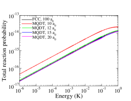
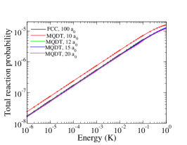
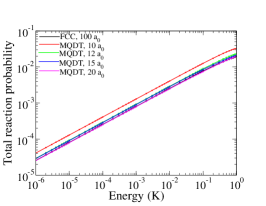
Figure 2: (Color online) Convergence of the total reaction probability in the $1\mu$K-1 K regime for different values of the short-range matching distance that defines the boundary between CC and MQDT formalisms. The left, middle and right panels correspond to $v=0,j=0$; $v=2,j=0$ and $v=5,j=0$ initial states of H₂, respectively. The different curves in each panel correspond to different matching distances for the MQDT part: 10 $a_{0}$ (red curve), 12 $a_{0}$ (green curve), 15 $a_{0}$ (blue curve), and 20 $a_{0}$ (pink curve).

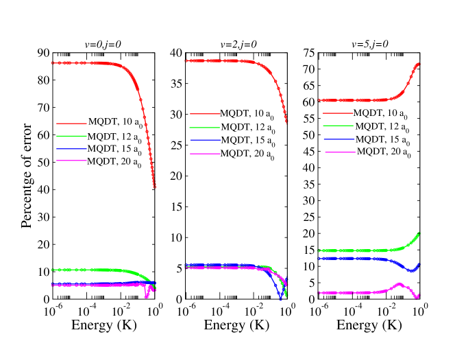
Figure 3: (Color online) The percentage error in total reaction probability for different short-range matching radii $S_{m}$ as a function of the collision energy for the three different initial ro-vibrational states of H₂ depicted in Fig 2.

Fig. 2 shows the convergence of the total reaction probabilities as a function of the short-range matching distance $S_{m}$ for three different initial vibrational levels of the H₂ molecule: $v=0,j=0$ (left panel); $v=2,j=0$ (middle panel) and $v=5,j=0$ (right panel). In each of the panels, results are shown for four different values of $S_{m}$: 10, 12, 15, and 20 $a_{0}$. In all three panels, the black curve shows converged full CC results obtained by matching at $\rho_{\infty}=100~{}a_{0}$. The different colored curves correspond to MQDT results for different values of $S_{m}$. It is seen that the hybrid CC-MQDT method yields nearly identical results as the numerically exact full CC calculation for a matching distance of 20 $a_{0}$. The percentage errors for the different matching distances are presented in Fig.3 for the different initial vibrational levels. While ideally one would like to have the smallest value of $S_{m}$ possible, any choice of $S_{m}$ at which the interaction potential has not reached its true asymptotic form will lead to larger errors as depicted by the results for $S_{m}$=10 $a_{0}$. Though any additional phase shift due to $V^{\rm lr}$ beyond $S_{m}$ is taken into account by MQDT, this phase shift is not taken into account for the reactive and vibrational de-excitation channels that are characterized by high kinetic energies and not described by MQDT. The percentage error is 30-80% for a matching radius of 10 $a_{0}$ (red curves) for all three vibrational levels. The percentage error is less than 10% for $S_{m}=12$ $a_{0}$ (green curves) and within 4-6% for $S_{m}=15$ and 20 $a_{0}$ (blue and pink curves). These values are slightly higher for $v=5$ for the matching radii of 12 and 15 $a_{0}$ but less than 5% for $S_{m}=20$ $a_{0}$. The convergence studies show that any values between 15-20 $a_{0}$ would be a reasonable short-range matching distance for MQDT.

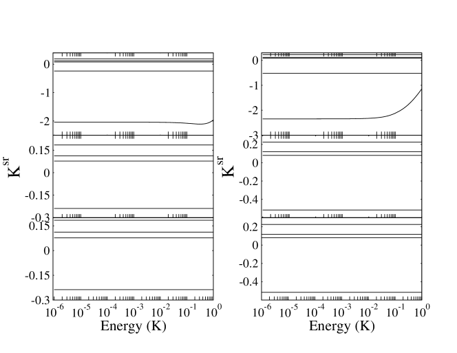
Figure 4: Diagonal elements of ${\bf K}^{\rm sr}$ involving only the reactant block as a function of energy for two different short-range matching distances. The left panel corresponds to a matching distance of 15 $a_{0}$ whereas the right panel pertains to the matching distance of 20 $a_{0}$.

III.1.2 Energy Independence of ${\bf K}^{\rm sr}$:

In Fig.4 we show the weak energy dependence of the diagonal elements of ${\bf K}^{\rm sr}$ as a function of the kinetic energy for two different matching distances of 15 (left panel) and 20 (right panel) $a_{0}$ for the $v=0,j=0$ initial state. It is clear from the left panel of Fig.4 that up to 100 mK the short range ${\bf K}$-matrix is independent of energy, but it becomes a smooth function of energy beyond 100 mK. This illustrates that, in principle, a single short-range ${\bf K}^{\rm sr}$-matrix can be used in the 1$\mu$K-100 mK regime, even though the cross sections vary by several orders of magnitude over this energy range. For energies in the 100 mK-1 K regime an interpolation procedure over a sparse grid of energies may be used. Thus, for the matching distance of 15 $a_{0}$, we divide the interpolation of $\bf{K^{\text{sr}}}$ into two different ranges of collision energy: (i) the ultra-low energy range $E_{c}=1\mu K$ - 1 mK, where ${\bf K}^{\rm sr}$ is evaluated at $1\mu$K and 1 mK and (ii) the energy range $E_{c}=$ 100 mK - 1 K, where an energy spacing of 200 mK is employed.

However, at $S_{m}=20$ $a_{0}$ (right panel of Fig.4) a stronger dependence on energy is observed for the same elements of ${\bf K}^{\rm sr}$ beyond 10 mK. This appears to be due to the very shallow nature of the van der Waals potential well in the D+H₂ system. The minimum of the van der Waals potential for D+H₂ is about 27 K at $S\approx 6.5$ $a_{0}$. As $S_{m}$ increases, the van der Waals well becomes shallower. At about 1 K the collision energy is no longer negligible compared to the well depth. Thus, the MQDT reference functions, defined by Eq. (21) and (22), become energy sensitive. This is also reflected in the stronger energy dependence of the ${\bf K}^{\rm sr}$ matrix obtained at $S_{m}=20~{}a_{0}$. Hence we need more points to accurately interpolate ${\bf K}^{\rm sr}$ evaluated at this matching distance. Therefore, in this case, we divide the interpolation of $\bf{K}^{\text{sr}}$ into three different ranges of collision energy: (i) the ultralow energy regime $E_{c}=1\mu$K - 1 mK, where ${\bf K}^{\rm sr}$ matrix is evaluated at $1\mu$K and 1 mK; (ii) the range $E_{c}$=10 mK-100 mK, where ${\bf K}^{\rm sr}$ is evaluated at 10 points with 10 mK separation; and (iii) the range $E_{c}=$ 200 mK - 1 K, where an energy spacing of 100 mK is employed. The energy dependence of ${\bf K}^{\rm sr}$ indicates that when the scattering energies are only a small fraction of the interaction potential (typically systems with deep attractive potential wells) a single ${\bf K}^{\rm sr}$ computed in the $\mu$K regime may suffice to evaluate reaction cross sections in the Kelvin regime. The results in Fig. 3 and 4 illustrate that 15 $a_{0}$ would be a resonable short-range matching radius for MQDT, and we adopt this value for the rest of the calculations.

The ability of MQDT to handle scattering in terms of an energy-smooth ${\bf K}^{\rm sr}$ will carry over into more elaborate conditions than the ones presented here. Notably, in the coldest collsions one may be interested in the influence of electronic and nuclear spin states on scattering, to say nothing of the ability of a magnetic field to manipulate scattering. This will require a description of Fano-Feshbach resonances, wherein the scattering observables will vary widely on the resonant scale. In MQDT, a whole forest of resonances may be usefully described over a large range of energy and field, utilizing a simple ${\bf K}^{\rm sr}$. Such resonances are not present in the prototype system we consider here, however.

III.2 Initial state-selected reaction probabilities and cross sections

In Fig. 5 we present a comparison of total reaction probabilities and the corresponding cross sections for D+H${}_{2}(v=0-7,j=0)$ collisions evaluated using the full CC and CC-MQDT approaches. Only the contribution from $J=0$ is included.

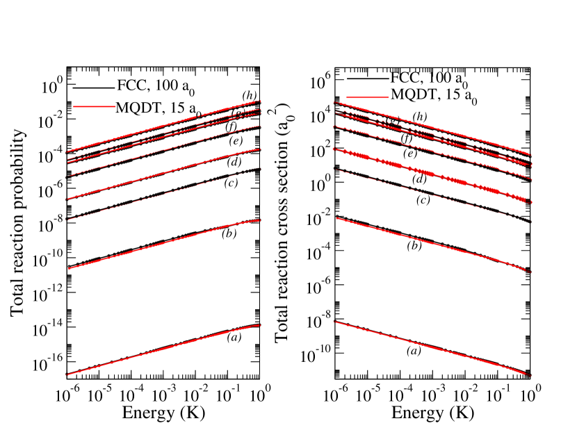
Figure 5: Total reaction probabilities (left panel) and the corresponding cross sections (right panel) for D+H${}_{2}(v,j)\to$HD+H reaction for $v=0-7$ and $j=0$ as functions of the incident collision energy. The black curves denote full CC results, and the overlapping red curves denote the corresponding MQDT results. The different curves correspond to the different initial vibrational levels of H₂: (a) $v=0$; (b) $v=1$; (c) $v=2$; (d) $v=3$; (e) $v=4$; (f) $v=5$; (g) $v=6$; and (h) $v=7$.

The full CC results are obtained at an asymptotic matching distance of 100 $a_{0}$; whereas, the MQDT results use a short-range matching distance of $S_{m}=15$ $a_{0}$. The different curves (in both the left and right panels) correspond to the different initial vibrational levels of the H₂ molecule. The solid black curves refer to results from full CC calculation, while the red curves correspond to MQDT results. The agreement between full CC and MQDT results is excellent, and in most cases the percentage error is about 5-6%. Since the reaction has an energy barrier of about 0.42 eV ($\sim$ 4800 K), the reaction probabilities are very small for $v=0$ and 1 initial states. However, the reactivity increases rapidly with H₂ vibrational excitation in agreement with previous results of Simbotin et al. Cote . The reactivity for $v=6$ and 7 are comparable to that of $v=5$. This is an indication that the reaction becomes essentially barrierless for $v\geq 5$. It is encouraging to see that, despite the small reactivity for $v=0$ and 1, the MQDT approach is still able to quantitatively reproduce the full CC results.

Regarding the parameters employed in the full CC calculations, stepsize of $\Delta\rho=0.01a_{0}$ is adopted for the radial integration. In the ABC code the total number of couple-channels is controlled by the three parameters $E_{\rm max}$, $j_{\rm max}$, and $\Omega_{\rm max}$. For a given $E_{\rm max}$, all channels with asymptotic rovibrational energies $\epsilon_{\tau vj}\leq E_{\rm max}$ are included, while the parameter $j_{\rm max}$ restricts the number of rotational levels for the different diatomic fragments. Similarly, $\Omega_{\rm max}$ ($k_{max}$ in the notation of ABC code) restricts the number of BF projection quantum numbers. Obviously, $\Omega_{max}=0$ for $J=0$. We have chosen different values of $E_{\rm max}$ for three different ranges of initial vibrational levels of H₂: for $v\leq 2$, $E_{\rm max}=3.5$ eV (this leads to $v_{\rm max}$=7 for H₂ and $v_{\rm max}$=8 for HD in the basis sets); for $3\leq v\leq 6$, $E_{\rm max}=4.25$ eV (this includes $v_{\rm max}$=10 for H₂ and $v_{\rm max}$=12 for HD) and for $v=7$, $E_{\rm max}=4.75$ eV (this includes $v_{\rm max}$=14 for H₂ and $v_{\rm max}$=17 for HD). However, we have restricted the total number of channels by fixing $j_{\rm max}=8$. Thus, the results presented here are only partially converged with respect to the number of rotational levels included in the basis set. Fully converged full CC results using higher rotational levels in the basis set have already been reported by Simbotin et al. Cote using the BKMP2 PES for the D+H₂ reaction for the vibrational levels and energy regimes investigated in this study. Since the aim of this paper is to illustrate the usefulness of the hybrid CC-MQDT formalism for cold and ultracold reactions, we resort to the smaller basis set described above.

III.3 Rovibrational-state resolution of reaction products

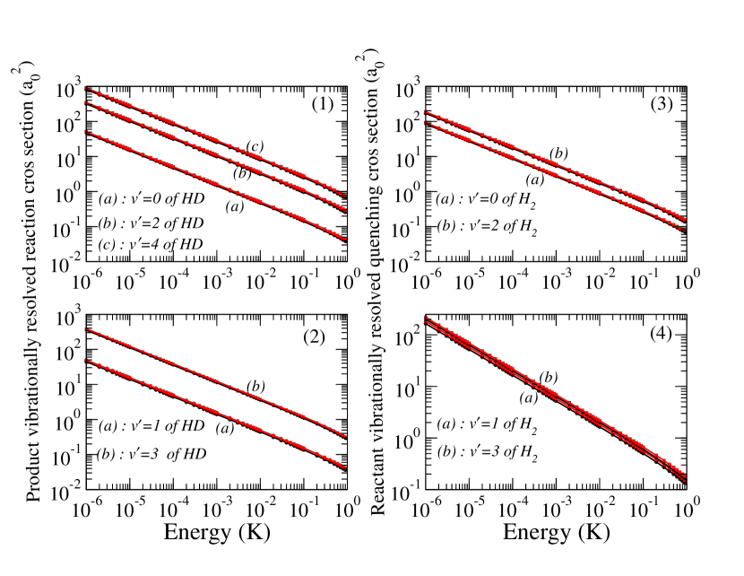
Figure 6: (Color online) Comparison between full CC and MQDT calculations for vibrationally resolved HD product as well as non-reactively scattered H₂ in D + H${}_{2}(v=4,j=0)$ collisions for total angular momentum $J=0$. The left panel shows vibrationally resolved cross sections for the HD product; whereas, the panel on the right shows corresponding cross sections for H₂ quenching.

The CC-MQDT approach presented here allows full quantum state resolution of reaction products as in full CC calculations, an aspect missing from previous MQDT treatments of ultracold chemistry. As an illustrative example we choose to study the $v=4,j=0$ initial state of H₂, which allows for the population of several rovibrational levels of the HD molecule as well as non-reactive quenching, leading to the population of lower vibrational levels of the reactant molecule. The total reaction probability and cross section for $J=0$ for this initial H₂ level have already been shown in Fig.5. In the left panels (1 and 2) of Fig.6, we show the corresponding vibrational-level resolved reaction cross sections for the HD product. Cross sections for non-reactive vibrational quenching of the H₂ molecule are shown in the right panels (3 and 4) of Fig.6. In all of the panels, the black curves denote the full CC results, and the red curves depict the MQDT results. The agreement is excellent, reflecting the similar agreement for the total cross sections.

The different curves correspond to the different vibrational levels of the HD product or non-reactively scattered H₂ molecule. Vibrational levels $v^{\prime}=0-4$ of the HD molecule are populated in the reaction. They are depicted by curves $(a)-(c)$ in panel (1) and $(a)$ and $(b)$ in panel (2) of Fig.6. The curves labeled $(a)$ and $(b)$ in panels (3) and (4) of Fig.6 show H₂ quenching cross sections. The results show that, even in the ultracold limit, chemical reaction dominates over inelastic vibrational quenching. The vibrationally resolved cross sections for quenching and reaction are proportional to the following sums: $\sigma^{v^{\prime}}_{\tau vj\Omega,\rm qn}\propto\sum_{{\rm qn},\hskip 2.84544ptj^{\prime}\Omega^{\prime}}|S^{v^{\prime}}_{\tau vj\Omega\to\tau v^{\prime}j^{\prime}\Omega^{\prime}}(E_{c})|^{2}$ and $\sigma^{v^{\prime}}_{\tau vj\Omega,\rm re}\propto\sum_{{\rm re},\hskip 2.84544ptj^{\prime}\Omega^{\prime}}|S^{v^{\prime}}_{\tau vj\Omega\to\tau^{\prime}v^{\prime}j^{\prime}\Omega^{\prime}}(E_{c})|^{2}$, respectively, where the sums are carried over all open rotational levels within a given vibrational level, $v^{\prime}$, of a particular arrangement channel. Note that here we omit the quantum number $J$ to simplify the notation.

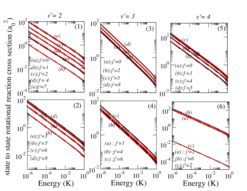
Figure 7: (Color online) Comparison between full CC and MQDT calculations for rotationally resolved reaction cross sections for the HD product in D + H${}_{2}(v=4,j=0)$ collisions. The left panels (1 and 2) correspond to HD$(v^{\prime}=2,j^{\prime})$, the middle panels (3 and 4) correspond to HD$(v^{\prime}=3,j^{\prime})$, and the right panels (5 and 6) correspond to HD$(v^{\prime}=4,j^{\prime})$.

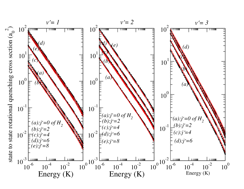
Figure 8: (Color Online) Similar results as in Fig.7 but for the non-reactively scattered H₂. The left panel corresponds to H${}_{2}(v^{\prime}=1,j^{\prime})$, the middle panel corresponds to H${}_{2}(v^{\prime}=2,j^{\prime})$, and the right panel corresponds to H${}_{2}(v^{\prime}=3,j^{\prime})$.

For vibrationally excited molecules, the treatment of MQDT is slightly modified in addition to the procedure described in Sec. IIB. For these cases, the MQDT-formalism is only applied to the initial collisional channel and those associated with cold and ultracold energies. Whereas, the other open inelastic (non-reactive) channels characterized by high kinetic energies within the reactant arrangement are treated in the standard way, i.e., these channels are matched to the normal asymptotic Bessel functions. In other words, they are treated like product channels. Thus, the transformations described by Eqs. (27) - (30) are also applied to the high kinetic energy channels of the reactant block in ${\bf\tilde{K}}_{\rm RR}$.

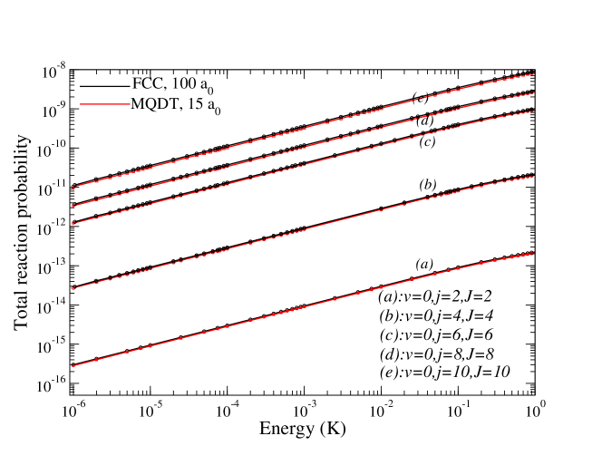
Figure 9: (Color online) Comparision of total reaction probability between the full CC and MQDT calculations as a function of collisional energy $E_{c}$ for an initially rotationally excited H₂ molecule within the $v=0$ vibrational level.

A comparison between the full CC and MQDT methods for rotationally resolved cross sections for the HD product in different energetically open vibrational levels are presented for the $v=4$ initial state in Fig. 7. The different panels correspond to the rotational distributions in the three highest populated vibrational levels, $v^{\prime}=2,3,$ and 4 of HD. As in other cases, the black curves denote the full CC results; whereas, the red curves depict the MQDT calculation. Again, the agreement is excellent, as it is in the case of vibrational distribution. Any small deviation can be attributed, at least in part, to neglecting the anisotropic contribution to the interaction potential in the construction of the MQDT reference functions.

The rotational level populations of non-reactively scattered H₂ molecules in three highest populated vibrational levels ($v^{\prime}=1,~{}2$ and 3) are presented in Fig.8. As before, the full CC results are shown by the black curves, and the MQDT-results are shown by the red curves. Note that only even rotational levels are populated since the calculations are restricted to the even parity states of the H₂ molecule (para-H₂).

III.4 Total reactive probability for non-zero $J$

Finally, in Fig.9 we present a comparison between full CC and MQDT results for the total reaction probability for different initial rotational levels of H₂ within the $v=0$ vibrational level. The different curves labeled (a)-(e) correspond to the initial rotational levels $j=2,~{}4,~{}6,8$ and 10, respectively. For each case, the calculations are restricted to $j=J$ to capture $s$-wave scattering in the incident channel. Also, for this particular case, both the triatomic parity $p$ and diatomic parity $q$ are limited to +1. These results are included to demonstrate that the method is not restricted to the non-rotating case.

IV Conclusions

We have presented a formulation of multichannel quantum defect theory that is able to yield full rovibrational level resolved cross sections and rate coefficients for cold and ultracold chemical reactions with an accuracy comparable to the full close-coupling calculations but at a much reduced computational cost. The method makes use of the close-coupling approach but restricts it to the chemically relevant region with the long-range part handled by the MQDT formalism. The usefulness and robustness of the method is illustrated by applying it to the benchmark D+H${}_{2}\to$ HD+H reaction for vibrational levels $v=0-7$ of the H₂ molecule. Rotational and vibrational populations of the product HD molecule are evaluated using this hybrid CC-MQDT method, and they are shown to be comparable to those obtained from the full close-coupling calculations. A similar agreement is found for rovibrational distributions of the non-reactively scattered H₂ molecule.

The method has many attractive features that make it appealing for ultracold chemical reactions. For instance, the short-range ${\bf K}$-matrix, evaluated by matching MQDT reference functions to the log-derivative matrix from the close-coupling calculation, is found to be largely energy independent in the $1\mu$K-10 mK regime. This implies that CC calculations need to be performed just at a single collision energy, say $1\mu$K, to evaluate cross sections at all energies between $1\mu$K-10 mK. Since this is the time consuming part of the computation, it leads to significant savings in computational time. For systems with deeper interaction potentials than D+H₂ (which has repulsive interaction at short range and a shallow van der Waals well in the long-range), the energy independence of the short-range ${\bf K}$-matrix is expected to be valid over a larger range of energies, allowing one to restrict the CC calculations to a few collision energies in the ultracold to 1-10 K regime. One caveat remains, namely, that the short-range ${\bf K}$-matrix may contain resonances from ro-vibrational channels that become closed at radial distances smaller than $S_{m}$ Hud1 , potentially requiring special handling within MQDT. Such resonances did not occur in the present calculation, however. Similarly, for open-shell systems with deep potential wells, calculations involving external fields, spin, and hyperfine effects can all be restricted to the MQDT part as energy splitting due to these factors will be many orders of magnitude smaller than the well depth of the interaction potential at short-range.

The application of the method to more complex reactions with deeper potential wells and inclusion of external field effects are planned.

V Acknowledgements

This work was supported in part by NSF grant PHY-1205838 (N.B.) and ARO MURI grant No. W911NF-12-1-0476 (N.B. and J.L.B). JH is grateful to Brian Kendrick for many helpful discussions.

APPENDIX-A

The matrix elements of the overlap matrix ${\bf O}$ between different arrangements $(\tau,\tau^{\prime})$ can be expressed in the SF representation as Krems

$$O_{\tau vj\ell,\tau^{\prime}v^{\prime}j^{\prime}\ell^{\prime}} = \frac{4}{\sin 2\theta_{\tau}\sin 2\theta_{\tau^{\prime}}}\langle\Upsilon_{\tau vj}(\theta_{\tau};\rho)|\langle{\cal Y}^{JM}_{j\ell}({\hat{s}}_{\tau},{\hat{S}}_{\tau})|\Upsilon_{\tau^{\prime}v^{\prime}j^{\prime}}(\theta_{\tau^{\prime}};\rho)\rangle|{\cal Y}^{JM}_{j^{\prime}\ell^{\prime}}({\hat{s}}_{\tau^{\prime}},{\hat{S}}_{\tau^{\prime}})\rangle$$ (A-1)

$$= \int d{\hat{S}_{\tau}}d{\hat{s}_{\tau}}\int^{\pi/2}_{0}d\theta_{\tau}{\cal Y}^{JM}_{j\ell}({\hat{s}}_{\tau},{\hat{S}}_{\tau}){\cal Y}^{JM}_{j^{\prime}\ell^{\prime}}({\hat{s}}_{\tau^{\prime}},{\hat{S}}_{\tau^{\prime}})$$

$$\times \left[\frac{\sin 2\theta_{\tau}}{\sin 2\theta_{\tau^{\prime}}}\right]\Upsilon_{\tau vj}(\theta_{\tau};\rho)\Upsilon_{\tau^{\prime}v^{\prime}j^{\prime}}(\theta_{\tau^{\prime}};\rho),$$

where the Jacobian, $\frac{1}{4}\sin^{2}2\theta_{\tau}$, for the integration over the angles is included in arriving at the second expression. The orthonormality of the matrix elements of ${\bf O}$ within the same arrangement, $(\tau,\tau)$ yields ${\bf O}_{\tau vj\ell,\tau v^{\prime}j^{\prime}\ell^{\prime}}=\delta_{vv^{\prime}}\delta_{jj^{\prime}}\delta_{\ell,\ell^{\prime}}$.

The matrix elements in the SF representation of the adibatic Hamiltonian are given by

$$\langle\xi_{m}|H_{\rm ad}(\rho)|\xi_{m^{\prime}}\rangle = \frac{4}{\sin 2\theta_{\tau}\sin 2\theta_{\tau^{\prime}}}\frac{1}{\sqrt{\sigma_{m}\sigma_{m^{\prime}}}}\sum_{\tau vj\ell}\sum_{\tau^{\prime}v^{\prime}j^{\prime}\ell^{\prime}}X_{\tau vj\ell,m}(\rho)X_{\tau^{\prime}v^{\prime}j^{\prime}\ell^{\prime},m^{\prime}}(\rho)$$ (A-2)

$$\times \langle\Upsilon_{\tau vj}(\theta_{\tau};\rho)|\langle{\cal Y}^{JM}_{j\ell}({\hat{s}}_{\tau},{\hat{S}}_{\tau})|H_{\rm ad}(\rho)|$$

$$\times \Upsilon_{\tau^{\prime}v^{\prime}j^{\prime}}(\theta_{\tau^{\prime}};\rho)\rangle|{\cal Y}^{JM}_{j^{\prime}\ell^{\prime}}({\hat{s}}_{\tau^{\prime}},{\hat{S}}_{\tau^{\prime}})\rangle.$$

In the SF representation, the sector-to-sector transformation matrix elements are defined by the following expression

$$[{\bf S}(\rho_{j},\rho_{j+1})]_{nn^{\prime}} = \langle\Phi^{JM}_{n}(\omega;\rho_{j})|\Phi^{JM}_{n^{\prime}}(\omega;\rho_{j+1})\rangle$$ (A-3)

$$= \sum_{m,m^{\prime}}F_{mn}(\rho_{j})F_{m^{\prime}n^{\prime}}(\rho_{j+1})\frac{1}{\sqrt{\sigma_{m}\sigma_{m^{\prime}}}}\sum_{\tau vj\ell}\sum_{\tau^{\prime}v^{\prime}j^{\prime}\ell^{\prime}}X_{\tau vj\ell,m}(\rho_{j})X_{\tau^{\prime}v^{\prime}j^{\prime}\ell^{\prime},m^{\prime}}(\rho_{j+1})$$

$$\times \frac{4}{\sin 2\theta_{\tau}\sin 2\theta_{\tau^{\prime}}}\langle\Upsilon_{\tau vj}(\theta_{\tau};\rho_{j})|\langle{\cal Y}^{JM}_{j\ell}({\hat{s}}_{\tau},{\hat{S}}_{\tau})|$$

$$\times \Upsilon_{\tau^{\prime}v^{\prime}j^{\prime}}(\theta_{\tau^{\prime}};\rho_{j+1})\rangle|{\cal Y}^{JM}_{j^{\prime}\ell^{\prime}}({\hat{s}}_{\tau^{\prime}},{\hat{S}}_{\tau^{\prime}})\rangle.$$

APPENDIX-B

Scattering Boundary Conditions

Once the propagation of the logderivative matrix from a small $\rho$ to an asymptotically large value of $\rho$ is accomplished, one needs to apply the asymptotic boundary conditions to the ${\bf Y}$ matrix (calculated in DC) to obtain ${\bf K}^{J}$. The boundary conditions are applied in Jacobi coordinates since the asymptotic forms of the wavefunctions are well known in this coordinate. Therefore, asymptotic analysis involves projecting the DC wavefunctions onto wavefunctions in Jacobi coordinates. A detailed description of this procedure is given by Pack and Parker Pack and only brief account is given below. Note that a similar approach will be used for matching MQDT reference functions to the log-derivative matrix from the CC calculations. First, in the asymptotic limit ($\rho\longrightarrow\infty$), where the exchange interactions between different arrangements become zero, it is convenient to express the total wavefunction $\Psi^{JM}$ of the reactive scattering system in Jacobi coordinates:

$$\Psi^{JM}=\sum_{\tau vj\ell}\frac{1}{s_{\tau}S_{\tau}}G^{J}_{\tau vj\ell}(S_{\tau}){\cal X}_{\tau vj}(s_{\tau}){\cal Y}^{JM}_{j\ell}({\hat{s}}_{\tau},{\hat{S}}_{\tau}),$$ (C-1)

where the quantities $G^{J}_{\tau vj\ell}$ and ${\cal X}_{\tau vj}$ denote, respectively, the radial expansion coefficients and the vibrational wavefunctions of the diatomic molecule. Note that here we explicitly include the quantum number $n=\{\tau,v,j,\ell\}$ since it refers to the asymptotic molecuar states. In the asymptotic region, the angular functions ${\cal Y}^{JM}_{j\ell}({\hat{s}}_{\tau},{\hat{S}}_{\tau})$ are the same in both Jacobi and DC as there is no overlap between functions with different $\tau$. The ro-vibrational wavefunctions in both coordinate systems satisfy the orthonormal condition. The asymptotic form of the total wavefunction in DC is given by

$$\Psi^{JM}=2\sum_{\tau vj\ell}\frac{\Gamma^{J}_{\tau vj\ell}(\rho)}{\rho^{5/2}}\frac{\Upsilon_{\tau vj}(\theta_{\tau};\rho)}{\sin 2\theta_{\tau}}{\cal Y}^{JM}_{j\ell}({\hat{s}}_{\tau},{\hat{S}}_{\tau}).$$ (C-2)

By usual projection and using the orthonormality of the ro-vibrational wave functions, the following expressions for the radial expansion coefficients, $\Gamma_{\tau vj\ell}^{J}(\rho)$ and its derivative, $\frac{\partial\Gamma_{\tau vj\ell}^{J}(\rho)}{\partial\rho}$ are obtained Pack

$$\Gamma_{\tau vj\ell}^{J}(\rho) = \frac{1}{4}\int_{0}^{\pi/2}d\theta_{\tau^{\prime}}(\sin 2\theta_{\tau^{\prime}})^{2}\int d{\hat{s}}_{\tau^{\prime}}d{\hat{S}}_{\tau^{\prime}}$$ (C-3)

$$\times \left[\frac{2\Upsilon_{\tau^{\prime}v^{\prime}j^{\prime}}^{*}(\theta_{\tau^{\prime}};\rho){\cal Y}^{JM*}_{j^{\prime}\ell^{\prime}}({\hat{s}}_{\tau^{\prime}},{\hat{S}}_{\tau^{\prime}})}{\sin 2\theta_{\tau^{\prime}}}\right]\left(\Psi^{JM}\rho^{5/2}\right)$$

$$\frac{\partial\Gamma_{\tau vj\ell}^{J}(\rho)}{\partial\rho} = \frac{1}{4}\int_{0}^{\pi/2}d\theta_{\tau^{\prime}}(\sin 2\theta_{\tau^{\prime}})^{2}\int d{\hat{s}}_{\tau^{\prime}}d{\hat{S}}_{\tau^{\prime}}$$ (C-4)

$$\times \left[\frac{2\Upsilon_{\tau^{\prime}v^{\prime}j^{\prime}}^{*}(\theta_{\tau^{\prime}};\rho){\cal Y}^{JM*}_{j^{\prime}\ell^{\prime}}({\hat{s}}_{\tau^{\prime}},{\hat{S}}_{\tau^{\prime}})}{\sin 2\theta_{\tau^{\prime}}}\right]\frac{\partial}{\partial\rho}\left(\Psi^{JM}\rho^{5/2}\right).$$

Using $sS=\rho^{2}\sin\theta\cos\theta=\frac{\rho^{2}\sin 2\theta}{2}$ and multiplying by $\rho^{5/2}$, Eq.(C-1) is reexpressed as

$$\rho^{5/2}\Psi^{JM}=\sum_{\tau vj\ell}\frac{2\rho^{1/2}}{\sin 2\theta_{\tau}}G^{J}_{\tau vj\ell}(S_{\tau}){\cal X}_{\tau vj}(s_{\tau}){\cal Y}^{JM}_{j\ell}({\hat{s}}_{\tau},{\hat{S}}_{\tau}).$$ (C-5)

Substitution of the above equation in Eqs. (C-3) and (C-4) and performing the integrals over $d{\hat{s}}_{\tau^{\prime}}$ and $d{\hat{S}}_{\tau^{\prime}}$ and using $\int d{\hat{s}}_{\tau^{\prime}}d{\hat{S}}_{\tau^{\prime}}{\cal Y}^{JM*}_{j^{\prime}\ell^{\prime}}({\hat{s}}_{\tau^{\prime}},{\hat{S}}_{\tau^{\prime}}){\cal Y}^{JM}_{j\ell}({\hat{s}}_{\tau},{\hat{S}}_{\tau})=\delta_{\tau^{\prime}\tau}\delta_{j^{\prime}j}\delta_{\ell^{\prime}\ell}$, one obtains

$$\Gamma_{\tau vj\ell}^{J}(\rho) = \sum_{\tau vj\ell}\delta_{\tau^{\prime}\tau}\delta_{j^{\prime}j}\delta_{\ell^{\prime}\ell}\rho^{1/2}\int_{0}^{\pi/2}d\theta_{\tau^{\prime}}\Upsilon_{\tau^{\prime},v^{\prime},j^{\prime}}^{*}(\theta_{\tau^{\prime}};\rho)G^{J}_{\tau vj\ell}(S_{\tau}){\cal X}_{\tau vj}(s_{\tau})$$ (C-6)

$$\frac{\partial\Gamma_{\tau vj\ell}^{J}(\rho)}{\partial\rho} = \frac{1}{2\rho}\Gamma_{\tau vj\ell}^{J}(\rho)+\sum_{\tau vj\ell}\delta_{\tau^{\prime}\tau}\delta_{j^{\prime}j}\delta_{\ell^{\prime}\ell}\rho^{1/2}$$ (C-7)

$$\times \int_{0}^{\pi/2}d\theta_{\tau^{\prime}}\Upsilon_{\tau^{\prime}vj}^{*}(\theta_{\tau^{\prime}};\rho)\frac{\partial[G^{J}_{\tau vj\ell}(S_{\tau}){\cal X}_{\tau vj}(s_{\tau})]}{\partial\rho}.$$

The asymptotic boundary conditions of the wavefunction and its derivative in Jacobi coordinates, in terms of two reference functions ${\bf\hat{f}}$ and ${\bf\hat{g}}$, are ${\bf G}(S_{\tau})={\bf\hat{f}}(S_{\tau})-{\bf\hat{g}}(S_{\tau})\bf K$ and ${\bf G^{\prime}}(S_{\tau})={\bf\hat{f}^{\prime}}(S_{\tau})-{\bf\hat{g}^{\prime}}(S_{\tau})\bf K$, respectively, where the primes indicate differentiation with respect to $S$, and $\bf K$ is the reactance matrix. In our case, the reference functions ${\bf\hat{f}}$ and ${\bf\hat{g}}$ are spherical Bessel functions in the product channels and MQDT-reference functions in the reactant channels. These two boundary conditions for the wavefunction $G$ in DC yields

$${\bf\Gamma}^{J}(\rho)={\bf{\cal A}}(\rho)-{\bf{\cal B}}(\rho){\bf K}^{J}$$

$$\frac{\partial{\bf\Gamma}^{J}(\rho)}{\partial\rho}=\frac{1}{2\rho}{\bf{\cal A}}(\rho)+{\bf{\cal C}}(\rho)-{\bf{\cal D}}(\rho){\bf K}^{J},$$ (C-8)

where the matrix elements of $\bf{\cal A}$ and $\bf{\cal C}$ have the form of

$${\cal A}_{\tau^{\prime}v^{\prime}j^{\prime}\ell^{\prime},\tau vj\ell}(\rho) = \delta_{\tau^{\prime}\tau}\delta_{j^{\prime}j}\delta_{\ell^{\prime}\ell}\rho^{1/2}\int_{0}^{\pi/2}d\theta_{\tau^{\prime}}\Upsilon_{\tau^{\prime}v^{\prime}j^{\prime}}^{*}(\theta_{\tau^{\prime}};\rho){\hat{f}}_{\tau vj\ell}(S_{\tau}){\cal X}_{\tau vj}(s_{\tau})$$ (C-9)

$${\cal C}_{\tau^{\prime}v^{\prime}j^{\prime}\ell^{\prime},\tau vj\ell}(\rho) = \delta_{\tau^{\prime}\tau}\delta_{j^{\prime}j}\delta_{\ell^{\prime}\ell}\rho^{1/2}\int_{0}^{\pi/2}d\theta_{\tau^{\prime}}\Upsilon_{\tau^{\prime}v^{\prime}j^{\prime}}^{*}(\theta_{\tau^{\prime}};\rho)$$ (C-10)

$$\times \left[\frac{d{\hat{f}}_{\tau vj\ell}}{dS_{\tau}}{\cal X}_{\tau vj}(s_{\tau})\cos\theta_{\tau}+\frac{d{\cal X}_{\tau vj}(s_{\tau})}{ds_{\tau}}{\hat{f}}_{\tau vj\ell}\sin\theta_{\tau}\right].$$

The matrices ${\bf{\cal B}}$ and ${\bf{\cal D}}$ have similar expressions but with the Bessel function ${\bf\hat{f}}(S)$ replaced by ${\bf\hat{g}}(S)$. It is clear from the expression of the projection matrices ${\bf{\cal A}}$ and ${\bf{\cal C}}$ that they are diagonal in all the quantum numbers but there is an overlap between different vibrational states with same $\{\tau,j,\ell\}$. From Eq.(24) and using the above expressions, the final form of the K-matrix is obtained in terms of the log-derivative matrix (in DC),

$${\bf K}^{J}=\left({\bf Y{\cal B}}-\frac{1}{2\rho}{\bf{\cal B}}-{\bf{\cal D}}\right)^{-1}\left({\bf Y{\cal A}}-\frac{1}{2\rho}{\bf{\cal A}}-{\bf{\cal C}}\right).$$ (C-11)

The S-matrix, ${\bf S}^{J}$ is obtained from the K-matrix using the well known Cayley transformation. It is to be noted that both ${\bf K}^{J}$ and ${\bf S}^{J}$ are independent of $\rho$ and the choice of the coordinate systems.

References

- (1) R. V. Krems, Int. Rev. Phys. Chem., 24, 99 (2005).
- (2) P. F. Weck and N. Balakrishnan, Int. Rev. Phys. Chem., 25 283 (2006).
- (3) P. Soldán and J. M. Hutson, Int. Rev. Phys. Chem., 25 497 (2006).
- (4) P. Soldán and J. M. Hutson, Int. Rev. Phys. Chem., 26 1 (2007).
- (5) R. V. Krems, Phys. Chem. Chem. Phys., 10 4079 (2008).
- (6) K.-K. Ni, S. Ospelkaus, M. H. G. de Miranda, A. Pe’er, B. Neyenhuis, J. J. Zirbel, S. Kotochigova, P. S. Julienne, D. S. Jin, and J. Ye, Science 322, 231 (2008).
- (7) S. Ospelkaus, K.-K. Ni, D. Wang, M. H. G. de Miranda, B. Neyenhuis, G. Quéméner, P. S. Julienne, J. L. Bohn, D. S. Jin, and J. Ye, Science 327, 853 (2010).
- (8) N. Balakrishnan and A. Dalgarno, Chem. Phys. Lett. 341, 652 (2001).
- (9) P. Soldán, M. T. Cvitaš, J. M. Hutson, P. Honvault, and J.-M. Launay, Phys. Rev. Lett. 89, 153201 (2002).
- (10) G. Quéméner, P. Honvault, and J.-M. Launay, Eur. Phys. J. D 30, 201 (2004).
- (11) M. T. Cvitaš, P. Soldán, J. M. Hutson, P. Honvault, and J.-M. Launay, Phys. Rev. Lett. 94, 200402 (2005).
- (12) J. C. Juanes-Marcos, G. Quéméner, B. K. Kendrick, and N. Balakrishnan, Phys. Chem. Chem. Phys. 13, 19067 (2011).
- (13) G. B. Pradhan, N. Balakrishnan and B. K. Kendrick, J. Chem. Phys. 138 164310 (2013).
- (14) T. V. Tscherbul and R. V. Krems, J. Chem. Phys. 129, 034112 (2008).
- (15) M. J. Seaton, Proc. Phys. Soc., 88, 801 (1966).
- (16) M. J. Seaton, Quantum defect theory, Rep. Prog. Phys., 46, 167 (1983).
- (17) U. Fano and A. R. P. Rau, Atomic Collisions and Spectra (Academic Press, Orlando, FL, 1986).
- (18) F. H. Mies, J. Chem. Phys. 80, 2514 (1984).
- (19) C. H. Greene, A. R. P. Rau, and U. Fano, Phys. Rev. A 26, 2441 (1982).
- (20) J. P. Burke, C. H. Greene, and J. L. Bohn, Phys. Rev. Lett. 81, 3355 (1998).
- (21) F. H. Mies and M. Raoult, Phys. Rev. A 62, 012708 (2000).
- (22) M. Raoult and F. H. Mies, Phys. Rev. A 70, 012710 (2004).
- (23) B. Gao, E. Tiesinga, C. J. Williams, and P. S. Julienne, Phys. Rev. A 72, 042719 (2005).
- (24) T. M. Hanna, E. Tiesinga, and P. S. Julienne, Phys. Rev. A 79, 040701 (2009).
- (25) B. P. Ruzic, C. H. Greene, and J. L. Bohn, Phys. Rev. A. 87, 032706 (2013).
- (26) Z. Idziaszek, T. Calarco, P. S. Julienne, and A. Simoni, Phys. Rev. A 79, 010702 (2009).
- (27) B. Gao, Phys. Rev. Lett. 104, 213201 (2010).
- (28) J. F. E. Croft, A. O. G. Wallis, J. M. Hutson, and P. S. Julienne, Phys. Rev. A 84, 042703 (2011).
- (29) J. F. E. Croft, J. M. Hutson, and P. S. Julienne, Phys. Rev. A 86, 022711 (2012).
- (30) Z. Idziaszek and P. S. Julienne, Phys. Rev. Lett. 104, 113202 (2010).
- (31) B. Gao, Phys. Rev. Lett., 105, 263203 (2010).
- (32) Z. Idziaszek, G. Quéméner, J. L. Bohn, and P. S. Julienne, Phys. Rev. A 82, 020703(R) (2010).
- (33) G.R. Wang, T. Xie, Y. Huang, W. Zhang, and S.L. Cong, Phys. Rev. A 86, 062704 (2012).
- (34) L. M. Delves, Nucl. Phys. 9, 391 (1959͒); 20, 275 (͑1960͒); F. T. Smith, Phys. Rev. 120, 1058 (͑1960͒).
- (35) R. T Pack and G. A. Parker, J. Chem. Phys. 87, 3888 (1987).
- (36) B. Lepetit, J. M. Launay and M. Le. Dourneuf, Chem. Phys. 106 103 (1986).
- (37) J. M. Launay and M. Le. Dourneuf, Chem. Phys. Letts. 163 178 (1989).
- (38) J. Hazra, B. P. Ruzic, N. Balakrishnan, and J. L. Bohn, Phys. Rev. A 90 032711 (2014).
- (39) D. Skouteris, J. F. Castillo, and D. E. Manolopoulos, Comp. Phys. Comm. 133, 128 (2000).
- (40) D. E. Manolopoulos, J. Chem. Phys. 85, 6425 (1986͒).
- (41) M. Tizniti, S. D. Le Picard, F. Lique, C. Berteloite, A. Canosa, M. H. Alexander, and I. R. Sims, Nature Chemistry, 6, 141 (2014).
- (42) S. L. Mielke, B. C. Garrett, and K. A. Peterson, J. Chem. Phys. 116, 4142 (2002).
- (43) I. Simbotin, S. Ghosal and R. Côté, Phys. Chem. Chem. Phys. 13, 19148 (2011).