Introduction

A symmetric, informationally complete, positive-operator valued measure or SIC-POVM on the Hermitian vector space $\mathbb{C}^{n}$ is a set $\{P_{j}\}$ of $n^{2}$ rank-one projection operators such that

$$\frac{1}{n}\!\sum_{i=1}^{n^{2}}P_{i}=I,$$

and

$$\mathop{\mathrm{tr}}(P_{j}P_{k})=\frac{1}{n+1}(n\delta_{jk}+1)$$

for all $j,k.$ Such objects attracted wide attention following conjectures about their existence made by Zauner Z in 1999 and Renes et al. RSC in 2004, and since then have been investigated by a large number of authors, along with higher rank versions and the allied concept of mutually unbiased basis. See, for example, App ; AFZ ; AYZ ; DBBA ; Durt ; Gour ; Grl ; Hogg ; Hugh ; SG ; Woo ; Zhu , and references cited therein.

SIC-POVMs arise in the theory of quantum measurement (see Davies Dav and Holevo Hol for the significance of general POVMs), and are of great interest in connection with their potential applications to quantum tomography. The idea is the following. Suppose that one has a large number of independent identical copies of a quantum system (say, a large molecule), the state (or ‘structure’) of which is unknown and needs to be determined. A SIC-POVM can be thought of as a kind of symmetrically oriented machine that can be used to make a single tomographic measurement on each independent copy of the molecule, with the property that once the results of the various measurements have been gathered for a sufficiently large number of molecules, the state of the molecule can be efficiently determined to a high degree of accuracy. The ‘symmetric orientation’ is not with respect to ordinary three-dimensional physical space (as in the classical tomography of medical imaging), but rather with respect to the space of pure quantum states.

Since each element $P_{i}$ of a SIC-POVM is a matrix of rank one and trace unity, it determines a point in complex projective space $\mathbb{CP}^{n-1}.$ It is well known that a SIC-POVM can then be defined as a configuration of $n^{2}$ points in $\mathbb{CP}^{n-1}$ that are mutually equidistant under the standard Kähler metric LS ; Wel . This is the definition that we shall adopt in §3, and the distance is determined by Lemma 3.6. Such a set of points is often called a ‘SIC’, but we favour the expression ‘SIC set’.

The existence of such configurations (for example, nine equidistant points in $\mathbb{CP}^{2},$ or sixteen equidistant points in $\mathbb{CP}^{3}$) is counterintuitive to our everyday way of thinking in which a regular simplex in $\mathbb{R}^{n}$ has $n+1$ vertices (but see GKMS ). It has been conjectured that $\mathbb{CP}^{n-1}$ possesses such a configuration for every $n$ RSC ; Z . There is evidence for this for $n$ up to at least $67,$ and various explicit solutions have been found in lower dimensions. Most of the known SIC sets in higher dimensions are constructed as orbits of a Heisenberg group $W\times H$ acting on $\mathbb{CP}^{n-1}$ (see Section 3), and representative vectors occur as eigenvectors of an isometry that is an outer automorphism of $W\times H.$ In the case $n=5$, the automorphisms of $W\times H$ play a key role in the construction of the celebrated Horrocks-Mumford bundle over $\mathbb{CP}^{4}$ in HM , which is an excellent reference for this group theory. In the case $n=3$ (and more generally, when $n$ is prime) any finite group of isometries whose orbit is a SIC set must be conjugate to $W\times H$ Zhu , but in this paper we work without the assumption of group covariance (see Grassl Grl ).

The space $\mathbb{CP}^{1},$ endowed with the Fubini-Study metric, is isometric to the standard two-sphere, and embedding this in $\mathbb{R}^{3}$ is a simple example of the representation of $\mathbb{CP}^{n-1}$ as an adjoint orbit in the Lie algebra $\mathfrak{su}(n)$ of its isometry group. The existence of a SIC set can then be interpreted as a statement about the placement of such orbits. The problem can also be formulated so as to apply to more general (co-)adjoint orbits in a Lie algebra.

The vertices of any inscribed regular tetrahedron in $S^{2}$ provide a SIC set for $\mathbb{CP}^{1}$ ($n=2$). The situation for the projective plane $\mathbb{CP}^{2}$ is already surprisingly intricate, and the case $n=3$ is characterized by the existence of continuous families of non-congruent SIC sets. It is easy to begin their study. Using homogeneous coordinates, any three equally-spaced points on the equator $\{[0,z_{2},z_{3}]:|z_{2}|=|z_{3}|\}$ of the two-sphere $z_{1}=0$ lie in a SIC set formed by adding three equally-spaced points from each of the equators of the two-spheres $z_{2}=0$ and $z_{3}=0.$ If the diameter of $\mathbb{CP}^{2}$ is chosen to be $\pi,$ all nine points are a distance $2\pi/3$ apart. Moreover, if the three triples match up so as to lie on a total of twelve projective lines, the nine points are the flexes of a plane cubic curve Hugh .

In this paper, we show that any SIC set in $\mathbb{CP}^{2}$ is congruent to one of those just described (see Theorem 5.5). This result will not surprise the experts; it has perhaps been verified numerically, and is apparently a consequence of computer-aided results in Sz . Our proof relies on a computation for its final step but is predominantly analytical. We use the two-point homogeneity of $\mathbb{CP}^{2}$ to fix two points of a SIC set; applying the moment mapping relative to a maximal torus shows that the remaining seven points lie in a pinched torus above a circle $\mathscr{C}$ in $\mathbb{R}^{3}$ (illustrated in Figure 1). We exhibit the known solutions in a different form (Proposition 6.2) and characterize them by a symmetry condition (Lemma 8.2). Adding three more points a distance $2\pi/3$ from the first two and from each other leads to a polynomial equation that is symmetric in three variables $x,y,z$ that represent the tangents of angles measured around $\mathscr{C}$ (Theorem 7.3). The resulting geometry is illustrated in Section 8.

Adding a sixth point allows us to write down four equations in four variables $t,x,y,z.$ When these are totally symmetrized, we obtain a system that represents a necessary condition for the six points to form part of a SIC set. For the known solutions, at least one of the four points on the pinched torus must project to $\mathscr{C}$ with an angle equal to $\pm\pi/6.$ This fact enables us to focus attention on the so-called quotient ideal that parametrizes ‘extra’ solutions, and to describe it by means of an appropriate Gröbner basis. Once one root $t$ is fixed, the extra solutions form a finite set and the final step is to determine its size. There are too few extra solutions for these to arise from an undiscovered SIC set.

This paper had its origins in a number of survey talks aimed at bringing elements of the SIC-POVM problem in various low dimensions to the attention of a wider audience, and the title and figures reflect this. We focus on the case $n=3$ from Section 4 onwards, and Sections 6–10 contain the more specialized material required to achieve our goal. The Fubini-Study metric on an ambient projective space plays a central role in the construction or approximation of Kähler-Einstein metrics on algebraic varieties, and it is our hope that more general theory may shed further light on the discrete problem outlined above.

1. Hermitian preliminaries

We begin with a few remarks to fix conventions. The complex vector space

(1.1) $$\mathbb{C}^{n}=\{\mathbf{z}=(z_{1},\ldots z_{n})^{\top}:z_{i}\in\mathbb{C}\}$$

of column vectors comes equipped with a Hermitian form

(1.2) $$\left<\mathbf{w},\mathbf{z}\right>=\left<\mathbf{w}|\,\mathbf{z}\right>=\sum_{i=1}^{n}\overline{w}_{i}z_{i}$$

which is anti-linear in the first (bra) position. Each fixed $\mathbf{w}$ defines a linear functional $\mathbf{z}\mapsto\left<\mathbf{w},\mathbf{z}\right>,$ and

(1.3) $$\mathbf{w}\ \mapsto\ \left<\mathbf{w},\ \hbox{\footnotesize$\bullet$}\ \right>$$

is an anti-linear bijective mapping $h\colon V\to V^{*},$ equivalently an isomorphism $V\cong\overline{V}^{*}$ of complex vector spaces. Complex projective space is the quotient

(1.4) $$\mathbb{CP}^{n-1}=\frac{\mathbb{C}^{n}\setminus 0}{\mathbb{C}^{*}},$$

consisting of one-dimensional subspaces of $\mathbb{C}^{n}$ or rays, and is a compact topological space. For any non-zero $\mathbf{w}\in\mathbb{C}^{n}$ the associated point in $\mathbb{CP}^{n-1}$ will be denoted by $[\mathbf{w}].$ Each such point determines a conjugate hyperplane $W$ defined by

(1.5) $$W=\mathbb{P}(\ker h(\mathbf{w}))\cong\mathbb{CP}^{n-2}\subset\mathbb{CP}^{n-1}.$$

This is the geometrical content of the map $h.$

Two points $[\mathbf{w}],[\mathbf{z}]$ lie on a unique projective line $\mathbb{L}\cong\mathbb{CP}^{1}.$ The associated conjugate hyperplanes $W,Z$ intersect $\mathbb{L}$ in $[\mathbf{w}^{\prime}],[\mathbf{z}^{\prime}],$ where

(1.6) $$\mathbf{w}^{\prime}=\left<\mathbf{w},\mathbf{z}\right>\mathbf{w}-\left<\mathbf{w},\mathbf{w}\right>\mathbf{z},\qquad\mathbf{z}^{\prime}=\left<\mathbf{z},\mathbf{z}\right>\mathbf{w}-\left<\mathbf{z},\mathbf{w}\right>\mathbf{z}.$$

The resulting four points, taken in the order $[\mathbf{w}],[\mathbf{z}],[\mathbf{z}^{\prime}],[\mathbf{w}^{\prime}],$ have inhomogeneous coordinates

(1.7) $$\infty,\quad 0,\quad-\big{<}\mathbf{z},\mathbf{z}\big{>}/\big{<}\mathbf{z},\mathbf{w}\big{>},\quad-\left<\mathbf{w},\mathbf{z}\right>/\big{<}\mathbf{w},\mathbf{w}\big{>},$$

and a real cross ratio

(1.8) $$\kappa([\mathbf{w}],[\mathbf{z}])=\frac{\big{<}\mathbf{w},\mathbf{z}\big{>}\big{<}\mathbf{z},\mathbf{w}\big{>}}{\big{<}\mathbf{w},\mathbf{w}\big{>}\big{<}\mathbf{z},\mathbf{z}\big{>}}=\frac{|\big{<}\mathbf{w},\mathbf{z}\big{>}|^{2}}{\|\mathbf{w}\|^{2}\|\mathbf{z}\|^{2}}\in[0,1].$$

When the points of $\mathbb{CP}^{n-1}$ are interpreted as pure quantum states, $\kappa$ can be regarded as a transition probability AshS ; BH ; Gib ; Hugh2 ; Hugh3 . The Fubini-Study distance $d$ between the points $[\mathbf{w}]$ and $[\mathbf{z}]$ is defined by expressing the cross ratio as $\cos^{2}(d/2),$ so that

(1.9) $$d([\mathbf{w}],[\mathbf{z}])=2\arccos\left(\frac{|\big{<}\mathbf{w},\mathbf{z}\big{>}|}{\|\mathbf{w}\|\|\mathbf{z}\|}\right)\in[0,\pi].$$

When $n=2$ we get $\mathbb{CP}^{1}\cong S^{2}.$ We shall see in Example 2.2 that $d$ is the spherical distance

(1.10) $$\theta=\arccos\big{|}\big{<}\mathbf{u},\mathbf{v}\big{>}\big{|},\qquad\mathbf{u},\mathbf{v}\in S^{2},$$

measuring the arclength of a great circle joining $\mathbf{u}$ and $\mathbf{v}.$ The $\mathbb{CP}^{1}$ calculation confirms that $d$ is the usual distance measured along geodesics of $\mathbb{CP}^{n-1}$ since any two points of the latter lie on a unique projective line $\mathbb{CP}^{1}.$ The distance (1.9) satisfies the triangle inequality

(1.11) $$d([\mathbf{w}],[\mathbf{z}])\leqslant d([\mathbf{w}],[\mathbf{y}])+d([\mathbf{y}],[\mathbf{z}]).$$

This can be verified by working inside the $\mathbb{CP}^{2}$ that contains $[\mathbf{w}],$ $[\mathbf{y}],$ $[\mathbf{z}].$

The so-called Fubini-Study metric is the square $ds^{2}$ of the infinitesimal distance between $[\mathbf{z}]$ and $[\mathbf{z}+d\mathbf{z}],$ computed using

(1.12) $$\begin{array}[]{rcl}\kappa([\mathbf{z}],[\mathbf{z}+d\mathbf{z}])&=&\displaystyle\frac{\|\mathbf{z}\|^{2}+2\mathop{\mathrm{Re}}\big{<}\mathbf{z},d\mathbf{z}\big{>}+|\big{<}\mathbf{z},d\mathbf{z}\big{>}|^{2}/\|\mathbf{z}\|^{2}}{\|\mathbf{z}\|^{2}+2\mathop{\mathrm{Re}}\big{<}\mathbf{z},d\mathbf{z}\big{>}+\|d\mathbf{z}\|^{2}}\\[20.0pt] &=&\displaystyle 1-\frac{\|d\mathbf{z}\|^{2}}{\|\mathbf{z}\|^{2}}+\frac{|\big{<}\mathbf{z},d\mathbf{z}\big{>}|^{2}}{\|\mathbf{z}\|^{4}}+O(\|d\mathbf{z}\|^{3}).\end{array}$$

There are no first-order terms, and we obtain the Riemannian metric $g=ds^{2}$ where

(1.13) $$ds^{2}\ =\ 4\frac{\|\mathbf{z}\|^{2}\|d\mathbf{z}\|^{2}-|\big{<}\mathbf{z},d\mathbf{z}\big{>}|^{2}}{\|\mathbf{z}\|^{4}}.$$

If we set $z_{n}=1,$ and use the summation convention over the remaining indices $z_{1},\ldots,z_{n-1},$ then in the traditional notation we have

(1.14) $$g_{\alpha\beta}dz^{\alpha}d\overline{z}^{\beta}\ =\ 4\frac{(\overline{z}_{\alpha}z^{\alpha}+1)dz_{\beta}d\overline{z}^{\beta}-\overline{z}_{\alpha}z_{\beta}dz^{\alpha}d\overline{z}^{\beta}}{(\overline{z}_{\alpha}z^{\alpha}+1)^{2}}.$$

See, for example, Arnold Arn and Kobayashi and Nomizu KN . When $n=2,$ we obtain the classical first fundamental form

(1.15) $$ds^{2}\ =\ \frac{4\,dzd\overline{z}}{(1+|z|^{2})^{2}}\ =\ \frac{8(dx^{2}+dy^{2})}{(1+x^{2}+y^{2})^{2}}$$

on the two-sphere $S^{2},$ in which $x,y$ are isothermal coordinates.

2. The special unitary group

The Hermitian form $h$ is invariant under the action of the unitary group

(2.1) $$\mathrm{U}(n)=\{X\in\mathbb{C}^{n,n}:\overline{X}\!X^{\top}=I\}.$$

Its centre consists of scalar multiples $e^{it}I$ that act trivially on $\mathbb{CP}^{n-1}.$ So we consider the special unitary group

(2.2) $$\mathrm{SU}(n)=\{X\in\mathrm{U}(n):\det X=1\},$$

whose centre is $\mathbb{Z}_{n}=\big{<}e^{2\pi i/n}I\big{>}.$ The next result is due to Wigner Wig ; a modern treatment is given in Fr .

Theorem 2.1.

The isometry group of the Fubini-Study space $\mathbb{CP}^{n-1},$ i.e. the group of bijections preserving the distance $d,$ is generated by $\mathrm{SU}(n)/\mathbb{Z}_{n}$ and $[\mathbf{z}]\mapsto[\overline{\mathbf{z}}].$

The Lie algebra $\mathfrak{su}(n)$ can (as a vector space) be defined as the tangent space $T_{I}\mathrm{SU}(n)$ at the identity. It consists of tangent vectors $A=\dot{X}_{0}$ to curves $X_{t}=I+tA+O(t^{2})$ in $U(n).$ Thus

(2.3) $$\mathfrak{su}(n)=\{A\in\mathbb{C}^{n,n}:\overline{A}+A^{\top}=0,\ \mathop{\mathrm{tr}}A=0\}.$$

A matrix $M\in\mathrm{SU}(n)$ acts on $\mathfrak{su}(n)$ by the adjoint representation

(2.4) $$A\mapsto M\!AM^{-1}=M\!AM^{\top}.$$

The space $\mathfrak{su}(n)$ carries an invariant inner product

(2.5) $$\big{<}A,B\big{>}=-\mathop{\mathrm{tr}}(AB),$$

and $\mathrm{SU}(n)$ itself carries a bi-invariant Riemannian invariant. We shall work with the corresponding affine space

(2.6) $$\mathscr{H}_{n}=\{A\in\mathbb{C}^{n,n}:\overline{A}=A^{\top},\ \mathop{\mathrm{tr}}A=1\}$$

of Hermitian matrices of trace one. There is an obvious bijection

(2.7) $$\mathscr{H}_{n}\ \stackrel{{\scriptstyle\cong}}{{\longrightarrow}}\ \mathfrak{su}(n),$$

given by $A\mapsto i(A-n^{-1}I).$

The canonical embedding of $\mathbb{CP}^{n-1}$ into $\mathscr{H}_{n}$ is a variant of the moment mapping for the adjoint action of $\mathrm{SU}(n).$ To describe it, assume for convenience that all vectors are normalized. Thus, we set $\|\mathbf{z}\|=1$ ($\mathbf{z}\in S^{2n-1}$) and there remains only a phase ambiguity in passing to a point $[\mathbf{z}]=[e^{it}\mathbf{z}]$ of $\mathbb{CP}^{n-1}.$ Map $[\mathbf{z}]$ to

(2.8) $$P_{\mathbf{z}}=\mathbf{z}\overline{\mathbf{z}}^{\top}=\textstyle\left(\begin{array}[]{l}|z_{1}|^{2}\quad z_{1}\overline{z}_{2}\quad z_{1}\overline{z}_{3}\cdots\\ z_{2}\overline{z}_{1}\quad|z_{z}|^{2}\quad z_{2}\overline{z}_{3}\cdots\\ z_{3}\overline{z}_{1}\quad\cdots\\ \cdots\quad\cdots\end{array}\right),$$

which is a projection operator (meaning $P^{2}=P$) of rank one. The injective map

(2.9) $$i\colon\mathbb{CP}^{n-1}\hookrightarrow\mathscr{H}_{n}$$

defined by $[\mathbf{z}]\mapsto P_{\mathbf{z}}$ is $\mathrm{SU}(n)$-equivariant. We can use it to measure distances since

(2.10) $$\kappa([\mathbf{w}],[\mathbf{z}])=\big{|}\big{<}\mathbf{w},\mathbf{z}\big{>}\big{|}^{2}=\mathop{\mathrm{tr}}(P_{\mathbf{w}}P_{\mathbf{z}}),$$

assuming $\|\mathbf{z}\|=1=\|\mathbf{w}\|.$ Moreover, the derivative

(2.11) $$i_{*}\colon T_{x}\mathbb{CP}^{n-1}\hookrightarrow T_{x}\mathscr{H}_{n}\cong\mathbb{R}^{N}$$

is $\mathrm{U}(n-1)$-equivariant, and (2.9) is an isometric embedding.

Example 2.2 (The Bloch sphere).

For $n=2,$ the image of this map consists of the matrices

(2.12) $$\left(\!\begin{array}[]{cc}|z_{1}|^{2}&\overline{z}_{1}z_{2}\\[3.0pt] z_{1}\overline{z}_{2}&|z_{2}|^{2}\end{array}\!\right)=\hbox{\Large$\frac{1}{2}$}\!\left(\!\begin{array}[]{cc}1+a&b+ic\\[2.0pt] b-ic&1-a\end{array}\!\right)$$

with $|z_{1}|^{2}+|z_{2}|^{2}=1$ and $a^{2}+b^{2}+c^{2}=1.$ This provides the well-known isomorphism $\mathbb{CP}^{1}\cong S^{2}.$ The angle $\theta$ between two unit vectors in $\mathbb{R}^{3}$ is given by

(2.13) $$aa^{\prime}+bb^{\prime}+cc^{\prime}=\cos\theta.$$

The inner product in $\mathscr{H}_{2}$ is then

(2.14) $$\textstyle\hbox{\Large$\frac{1}{2}$}(1+aa^{\prime}+bb^{\prime}+cc^{\prime})=\hbox{\Large$\frac{1}{2}$}(1+\cos\theta)=\cos^{2}(\theta/2).$$

But $\theta$ is also the standard distance $d$ along the great circle on the surface of the sphere joining the endpoints of the two unit vectors.

In the example above, fix (say) the north pole $p\in S^{2},$ and consider the function $\kappa_{p}=\sin^{2}(\theta/2)$ where $\theta$ is now latitude in radians. Its gradient $\nabla\kappa_{p}$ is tangent to the meridians joining $p$ to the south pole $p^{\prime},$ whereas $J(\nabla\kappa_{p})$ is a vector field that represents rotation about $pp^{\prime}.$ This situation is generalized to higher dimensions as follows. The composition

(2.15) $$\mathbb{CP}^{n-1}\ \longrightarrow\ \mathscr{H}_{n}\ \stackrel{{\scriptstyle\cong}}{{\longrightarrow}}\ \mathfrak{su}(n),$$

where $[\mathbf{z}]\mapsto i(P_{\mathbf{z}}-n^{-1}I),$ is a moment mapping of the type determined whenever a Lie group acts on a symplectic manifold. The image (isomorphic to $\mathbb{CP}^{n-1}$) inside $\mathfrak{su}(n)$ is an orbit for the action of $\mathrm{SU}(n).$ Any such adjoint orbit carries a Kähler metric by general principles. Fix a point $p=[\mathbf{z}]\in\mathbb{CP}^{-1},$ and consider the function $\kappa_{p}$ defined by

(2.16) $$\kappa_{p}([\mathbf{w}])=\kappa([\mathbf{z}],[\mathbf{w}])=\mathop{\mathrm{tr}}(P_{\mathbf{z}}P_{\mathbf{w}}).$$

We have

Proposition 2.3.

The rotated gradient $J(\nabla\kappa_{p})$ is the infinitesimal isometry (Killing field) associated to $i(P_{\mathbf{z}}-n^{-1}I).$

For further details of various aspects of the Kählerian geometry of the space of pure quantum states, see Anandan and Aharonov AA , Ashtekar and Schilling AshS , Bengtsson and Zyczkowski BZ , Brody and Hughston BH , Gibbons Gib , Hughston Hugh2 ; Hugh3 , and Kibble Kib .

3. Sets of points in projective space

We choose to begin with

Definition 3.1.

A SIC-POVM or SIC set is a collection $\SS$ of $n^{2}$ points $[\mathbf{z}_{i}]$ in $\mathbb{CP}^{n-1}$ that are mutually equidistant, so if $\|\mathbf{z}_{i}\|=1$ then

(3.1) $$|\big{<}\mathbf{z}_{i},\mathbf{z}_{j}\big{>}|^{2}=\kappa,\qquad i\neq j,$$

for some fixed cross ratio $\kappa\in[0,1).$

We can associate to $[\mathbf{z}_{i}]$ the point $P_{i}=P_{[\mathbf{z}_{i}]}$ in $\mathscr{H}_{n}.$ A SIC set then consists of a regular simplex embedded in

(3.2) $$\mathscr{H}_{n}\cong\mathfrak{su}(n)\cong\mathbb{R}^{N},\quad N=n^{2}\!-\!1$$

with $n^{2}$ vertices $\{P_{i}\}$ that lie in the adjoint orbit $\mathbb{CP}^{n-1}.$ The latter requirement is the crucial one, since a regular simplex with $n^{2}$ vertices in $\mathbb{R}^{N}$ is readily obtained by projecting an arbitrary orthonormal basis of $\mathbb{R}^{N+1}.$

Do SIC sets exist?

Example 3.2.

A SIC set in $\mathbb{CP}^{1}=S^{2}$ is an inscribed tetrahedron in the two-sphere. Any two such tetrahedrons are congruent by $\mathrm{SO}(3)=\mathrm{SU}(2)/\mathbb{Z}_{2},$ though that does not stop us seeking the ‘neatest’ set of vertices to write down. One set is

(3.3) $$\Big{\{}\ [0,1],\quad[\sqrt{2},1],\quad[\sqrt{2},\omega],\quad[\sqrt{2},\omega^{2}]\ \Big{\}},$$

where $\omega=e^{2\pi i/3}.$ Another set of vertices, which is perhaps less obvious, is

(3.4) $$\Big{\{}\ [1,\varpi],\quad[\varpi,1],\quad[1,-\varpi],\quad[\varpi,-1]\ \Big{\}},$$

where $\varpi=(1+i)/(1+\sqrt{3}).$ This second set nevertheless plays an important role, as we shall see.

If $n\geqslant 3,$ any two SIC sets in $\mathbb{CP}^{n-1}\subset\mathbb{R}^{N}$ are congruent by $\mathrm{SO}(N)$ (where $N=n^{2}-1$), but not in general by $\mathrm{SU}(n).$

One can present more SIC sets by generalizing the second tetrahedron (3.4). We define two cyclic groups of order $n.$ Let $W$ be the group generated by the cyclic permutation

(3.5) $$[z_{1},z_{2},\ldots,z_{n}]\mapsto[z_{n},z_{1},\ldots,z_{n-1}];$$

let $\omega=e^{2\pi i/n},$ and denote by $H$ the group generated by

(3.6) $$[z_{1},z_{2},\ldots,z_{n}]\mapsto[z_{1},\omega z_{2},\ldots,\omega^{n-1}z_{n}].$$

$W\times H$ acts on $\mathbb{CP}^{n-1}$ as a subgroup of $\mathrm{SU}(n)$ isomorphic to $\mathbb{Z}_{n}\times\mathbb{Z}_{n}.$ This subgroup is sometimes called the Weyl-Heisenberg group after Weyl . It can be regarded as the projectivization of an extended finite group, namely the Heisenberg group of three-by-three matrices with coefficients in the ring $\mathbb{Z}_{n}.$ For this reason, it is legitimate to refer to the action of $W\times H$ simply as that of the Heisenberg group. The following two results can be verified by direct calculation:

Proposition 3.3.

The orbit

(3.7) $$(W\times H)\cdot[0,1,1]$$

is a SIC set consisting of nine points in $\mathbb{CP}^{2}.$

Proposition 3.4.

Let $r=\sqrt{2}$ and $s=\sqrt{2+\sqrt{5}}.$ Then

(3.8) $$(W\times H)\cdot[-s-i(r\!+\!s),\ 1\!-\!r+i,\ s+i(s\!-\!r),\ 1+r+i]$$

is a SIC set of sixteen points in $\mathbb{CP}^{3}.$

An element $\mathbf{z}\in\mathbb{C}^{n}$ such that the orbit $(W\times H)\cdot[\mathbf{z}]$ is a SIC set is called a fiducial vector for the action of $W\times H.$

In his 1999 Vienna PhD thesis Z , Zauner made a number of conjectures that extended the basic

Conjecture 3.5.

$\mathbb{CP}^{n-1}$ possesses a SIC set for all $n.$

It is widely believed that such a set can always be realized as an orbit of $W\times H,$ and that the number of non-congruent solutions (meaning solutions that are not related to one another by an isometry or element of $\mathrm{SU}(n)$) increases with $n.$ There are sporadic constructions of SIC sets using different finite groups (see Remark 3.8).

Explicit algebraic solutions are known for $n=2,3,4,\ldots,15,19,24,35$ and $48,$ from work of Zauner Z , Appleby App , Renes et al. RSC , Flammia Fla , Grassl Grl , Zhu Zhu , and many other authors (see AFZ ; DBBA and references cited therein). All such examples lie (up to isometry) in solvable extensions of $\mathbb{Q}$ AYZ . Extensive numerical verification has been carried out for $n\leqslant 67$ (Scott and Grassl SG ).

The next result is well known, but we include it for completeness. Let $\{[\mathbf{z}_{i}]\}$ be a SIC set in $\mathbb{CP}^{n-1}$ and $\{P_{i}\}$ its image in $\mathscr{H}_{n}.$ Recall that $\mathop{\mathrm{tr}}(P_{i}P_{j})=\kappa$ if $i\neq j.$ Thus $\kappa$ is the cross ratio or transition probability between any two points in the SIC set.

Lemma 3.6.

Any SIC set in $\mathbb{CP}^{n-1}$ satisfies $\kappa=1/(n+1),$ and

(3.9) $$\frac{1}{n}\sum P_{i}=I.$$

Proof.

Define $Q_{j}=P_{j}-\kappa I.$ Then

(3.10) $$\mathop{\mathrm{tr}}(P_{i}Q_{j})=\left\{\begin{array}[]{ll}1-\kappa&i=j\\ 0&i\neq j\end{array}\right.$$

So $(P_{i})$ is a basis of $i\mathfrak{u}(n)$ (called a quorum) and we can set

(3.11) $$I=\sum_{i=1}^{n^{2}}c_{i}P_{i}.$$

Applying $\mathop{\mathrm{tr}}(Q_{j}\,\cdot),$ we get $1-\kappa n=c_{j}(1-\kappa),$ so all the $c_{i}$ are equal. To complete the proof, take the trace of (3.11). This gives

(3.12) $$n=n^{2}\frac{1-\kappa n}{1-\kappa},$$

and $\kappa=(1-n)/(1-n^{2})=1/(1+n).$ ∎

It will be convenient in our analysis of SIC sets to introduce the following.

Definition 3.7.

Two points in $\mathbb{CP}^{n-1}$ will be said to be ‘correctly separated’ if the cross ratio that they define equals $1/(n+1).$

Suppose that $\mathbb{CP}^{n-1}$ admits a SIC set $\SS.$ Then, up to isometry, two points form part of a SIC set if and only if they are correctly separated. This follows from the fact that $\mathbb{CP}^{n-1}$ is a two-point homogeneous space, meaning that there exists an isometry that maps any two points to any other two points the same distance apart Wang . The lemma above is then a key result that enables one to go some way in attempting to construct a SIC set without knowing for sure that it exists.

Remark 3.8.

Lemma 3.6 precludes the existence of four or more points of a SIC set from lying on a projective line $\mathbb{CP}^{1}$ whenever $n\geqslant 3,$ since their cross ratio would have to be that for $n=2,$ namely $1/3.$ An application relates to the SIC set in $\mathbb{CP}^{7}$ constructed by Hoggar Hogg . It consists of a $(\mathbb{Z}_{2})^{6}$ orbit of 64 points that the Hopf fibration $\pi\colon\mathbb{CP}^{7}\to\mathbb{HP}^{3}$ projects down to an equal number of points in the quaternionic projective space $\mathbb{HP}^{3}.$ It would be impossible to find a SIC set in $\mathbb{CP}^{7}$ with four points in each fibre of $\pi,$ but we wonder whether there exists a SIC set arising from 32 points in $\mathbb{HP}^{3}$ with two points in each fibre. Such questions are related to work by Armstrong et al. on twistor lifts APS .

4. The action of a maximal torus

Starting in this section, we restrict the discussion mainly to the case $n=3.$ We shall develop the concept of moment mapping, but restricted to a maximal torus in $\mathrm{SU}(3),$ acting on $\mathbb{CP}^{2}.$ Fix the torus

(4.1) $$T=\left\{\left(\!\begin{array}[]{ccc}e^{ix_{1}}&0&0\\ 0&e^{ix_{2}}&0\\ 0&0&e^{ix_{3}}\end{array}\!\right)\ :\ \textstyle\sum\limits_{i=1}^{3}x_{i}=0\hbox{ mod\,$2\pi$}\right\},$$

which is, of course, homeomorphic to $S^{1}\times S^{1}.$ The hyperplane $x_{1}+x_{2}+x_{3}=0$ in $\mathbb{R}^{3}$ represents the Lie algebra $\mathfrak{t}$ of $T,$ which we also identify with $\mathfrak{t}^{*}$ using the induced inner product. The moment mapping for $T$ acting on $\mathbb{CP}^{2}$ is then the composition

(4.2) $$\mathbb{CP}^{2}\longrightarrow\mathfrak{su}(3)\longrightarrow\mathfrak{t}$$

obtained by projecting the adjoint orbit orthogonally to $\mathfrak{t}.$

When we pass from $\mathfrak{su}(3)$ to $\mathscr{H}_{3}$ via (2.7), we can identify this composition with the mapping $[\mathbf{z}]\mapsto(x_{1},x_{2},x_{3}),$ where

(4.3) $$(x_{1},x_{2},x_{3})=\mu([\mathbf{z}])=\frac{1}{\|\mathbf{z}\|^{2}}(|z_{1}|^{2},|z_{2}|^{2},|z_{3}|^{2})$$

consists of the diagonal entries in (2.8). Here, $\|\mathbf{z}\|^{2}=|z_{1}|^{2}+|z_{2}|^{2}+|z_{3}|^{2},$ though it is convenient to assume $\|\mathbf{z}\|=1.$ After the shift from traceless matrices to $\mathscr{H}_{3},$ the image of $\mu$ is the two-simplex $\mathscr{T},$ a filled equilateral triangle lying in the plane $x_{1}+x_{2}+x_{3}=1,$ illustrated in Figure 1. The residual three-fold symmetry visible is that of the Weyl group $W=N(T)/T\cong\mathbb{Z}_{3}.$

It is well known that $\mathscr{T}$ parametrizes the orbits of $T$ on $\mathbb{CP}^{2}$ via (4.3). See, for example, Guillemin and Sternberg GS . The inverse image of an interior point of $\mathscr{T}$ is a two-torus $T/\mathbb{Z}_{3};$ the inverse image of a vertex is a single point in $\mathbb{CP}^{2};$ and the inverse image of any other boundary point is a circle $S^{1}.$ Topologically, this leads to a description of the complex projective plane as a quotient

(4.4) $$\mathbb{CP}^{2}=\frac{\mathscr{T}\times T^{2}}{{}\sim{}}.$$

Here $\sim$ is the equivalence relation that collapses points over the boundary of $\mathscr{T}$ in accordance with the scheme outlined above.

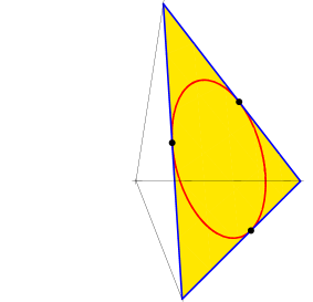
Figure 1. The image of the moment mapping $\mu\colon\mathbb{CP}^{2}\to\mathbb{R}^{3}$ is a two-simplex $\mathscr{T}$ that takes the form of a filled equilateral triangle. If $\mathbf{z}=(z_{1},z_{2},z_{3})$ is a unit vector in $\mathbb{C}^{3},$ the point $[\mathbf{z}]$ is mapped to $(x_{1},x_{2},x_{3})=(|z_{1}|^{2},|z_{2}|^{2},|z_{3}|^{2}).$ The inscribed circle is the intersection of the plane $x_{1}+x_{2}+x_{3}=1$ containing the (coloured) image of $\mu$ and the (invisible) sphere $x_{1}^{2}+x_{2}^{2}+x_{3}^{2}=\frac{1}{2}.$

Let $m_{1},m_{2},m_{3}$ be the midpoints of the sides of $\mathscr{T},$ and consider the circles

(4.5) $$C_{i}=\mu^{-1}(m_{i}),\qquad i=1,2,3.$$

The first circle $C_{1}$ consists of those points $[0,z_{2},z_{3}]$ of $\mathbb{CP}^{2}$ with $|z_{2}|=|z_{3}|.$ Any set of three equidistant points in $C_{1}$ has the form

(4.6) $$[0,e^{i\sigma},1],\quad[0,e^{i\sigma},\omega],\quad[0,e^{i\sigma},\omega^{2}],$$

where $\omega=e^{2\pi i/3}.$ The cross ratio defined by any two of these points is given by

(4.7) $$\textstyle\left|\frac{1}{2}(1+\omega)\right|^{2}=\frac{1}{4},$$

so they are indeed correctly separated. Similarly, $C_{2}$ consists of points $[z_{1},0,z_{3}]$ with $|z_{1}|=|z_{3}|,$ and $C_{3}$ points $[z_{1},z_{2},0]$ with $|z_{1}|=|z_{2}|.$ Now choose three equidistant points in $C_{2},$ and three equidistant ones in $C_{3}.$ It is easy to check that the resulting nine points constitutes a SIC set. This generalizes Proposition 3.3.

Definition 4.1.

By a midpoint solution, we mean a SIC set in $\mathbb{CP}^{2}$ consisting of three points in each of the three circles $C_{1},C_{2},C_{3}.$

This construction defines a one-parameter family of SIC sets up to isometry, since the stabilizer in $\mathrm{SU}(3)$ of the points in $C_{1}$ is a subgroup $\mathrm{U}(1)$ that can be used to remove the phase ambiguity in $C_{2}.$ See the discussion surrounding (6.10).

Let $\mathscr{C}$ denote the circle passing through the midpoints $m_{1},m_{2},m_{3},$ illustrated in Figure 1. As a curve in $\mathbb{R}^{3},$ it is the intersection of the plane $x_{1}+x_{2}+x_{3}=1$ with the sphere $x_{1}^{2}+x_{2}^{2}+x_{3}^{2}=1/2.$ It was actually plotted using the next result.

Lemma 4.2.

In $\mathbb{R}^{3},$ the inscribed circle $\mathscr{C}$ is parametrized by

(4.8) $$\hbox{\Large$\frac{2}{3}$}\Big{(}\!\cos^{2}\theta,\,\cos^{2}(\theta+\hbox{\Large$\frac{2}{3}$}\pi),\,\cos^{2}(\theta+\hbox{\Large$\frac{4}{3}$}\pi)\Big{)},$$

for $\theta\in[-\frac{1}{2}\pi,\frac{1}{2}\pi).$

Proof.

First, consider the effect of $\mu$ on real vectors. Suppose that $\mathbf{z}=(a,b,c)$ is a unit vector with $a,b,c\in\mathbb{R},$ and set $s_{k}=a^{k}+b^{k}+c^{k}.$ There is an identity

(4.9) $$s_{1}(-a+b+c)(a-b+c)(a+b-c)=s_{2}^{2}-2s_{4}.$$

If $\mu([\mathbf{z}])=(a^{2},b^{2},c^{2})\in\mathscr{C}$ then $s_{2}=1$ and $s_{4}=1/2,$ so the right-hand side of (4.9) vanishes. It follows $a\pm b\pm c=0$ for some choice of signs. Now set

(4.10) $$\textstyle a=\sqrt{\frac{2}{3}}\cos\theta,\quad b=\sqrt{\frac{2}{3}}\cos(\theta+\hbox{\Large$\frac{2}{3}$}\pi),\quad c=\sqrt{\frac{2}{3}}\cos(\theta+\hbox{\Large$\frac{4}{3}$}\pi).$$

Trig-expanding $b$ and $c$ shows that $a+b+c=0$ and $a^{2}+b^{2}+c^{2}=1.$ It follows from (4.9) that $s_{4}=1/2$ and $(a^{2},b^{2},c^{2})\in\mathscr{C}.$

The midpoints $m_{1},m_{2},m_{3}$ are given respectively by $\theta=\pm\pi/2,-\pi/6,\pi/6.$ This confirms the stated range for $t.$ ∎

5. Weyl-Heisenberg orbits

In this section, we show how the moment mapping (4.3) helps one to understand the action of the groups $W$ and $H$ defined in (3.5) and (3.6) with $n=3.$ We shall see that the $\mathscr{C}$ plays a prominent role, and Lemma 4.2 will be the basis for the parametrization of elements of a SIC set.

Lemma 5.1.

The $H$-orbit of a point $[\mathbf{z}]$ in $\mathbb{CP}^{2}$ consists of three points that are correctly separated from one another if and only if $\mu([\mathbf{z}])\in\mathscr{C}.$

Proof.

Suppose that $\mathbf{z}=\mathbf{z}^{(0)}$ is a unit vector. The orbit $H\cdot[\mathbf{z}]$ consists of the projective classes of the vectors

(5.1) $$\mathbf{z}^{(0)}=(z_{1},z_{2},z_{3}),\quad\mathbf{z}^{(1)}=(z_{1},\omega z_{2},\omega^{2}z_{3}),\quad\mathbf{z}^{(2)}=(z_{1},\omega^{2}z_{2},\omega z_{3})$$

generated by (3.6). We can express

(5.2) $$|\big{<}\mathbf{z}^{(0)},\mathbf{z}^{(1)}\big{>}|^{2}=(|z_{1}|^{2}+\omega|z_{2}|^{2}+\omega^{2}|z_{3}|^{2})(|z_{1}|^{2}+\omega^{2}|z_{2}|^{2}+\omega|z_{3}^{2}|)$$

in the form $\alpha-\beta,$ where

(5.3) $$\alpha=|z_{1}|^{4}+|z_{2}|^{4}+|z_{3}|^{4},\quad\beta=|z_{2}|^{2}|z_{3}|^{2}+|z_{3}|^{2}|z_{1}|^{2}+|z_{1}|^{2}|z_{2}|^{2}.$$

Therefore $\mathbf{z}^{(0)}$ and $\mathbf{z}^{(1)}$ are correctly separated if and only if $\alpha-\beta=1/4.$ But

(5.4) $$\alpha+2\beta=(|z_{1}|^{2}+|z_{2}|^{2}+|z_{3}|^{2})^{2}=1,$$

since $\mathbf{z}=\mathbf{z}^{(0)}$ is normalized, so the condition of correct separation is $\alpha=1/2.$ Since $x_{i}=|z_{i}|^{2}$ are the Cartesian coordinates in $\mathbb{R}^{3},$ correct separation of $\mathbf{z}^{(0)}$ and $\mathbf{z}^{(1)}$ implies that $\mu([\mathbf{z}])\in\mathscr{C}.$ This condition only depends on $\mu([\mathbf{z}])$ since $H$ is a subgroup of $T$ and its action commutes with all the elements of $T.$ Therefore if $\mu([\mathbf{z}])\in\mathscr{C},$ all three points in (5.1) will be correctly separated. ∎

Example 5.2.

Lemma 5.1 is really an assertion about the induced metric on the fibres $\mu^{-1}(p)$ for $p\in\mathscr{C}.$ This metric will depend crucially on the position of $p$ in $\mathscr{C},$ since it degenerates as $p$ approaches any one of the midpoints $m_{i}$ (over which the fibres are circles rather than 2-tori). This behaviour is illustrated in Figure 2, which provides a visualization of the fibres $\mu^{-1}(p_{i})$ for $i=1,2,$ where

(5.5) $$p_{1}=\big{(}\hbox{\Large$\frac{2}{3}$},\hbox{\Large$\frac{1}{6}$},\hbox{\Large$\frac{1}{6}$}\big{)},\qquad p_{2}=\big{(}\hbox{\Large$\frac{1}{8}$}(3+\sqrt{5}),\hbox{\Large$\frac{1}{4}$},\hbox{\Large$\frac{1}{8}$}(3-\sqrt{5})\big{)}.$$

are two points of $\mathscr{C}$. Note that $p_{1}$ is the point diametrically opposite $m_{1},$ whereas $p_{2}$ lies between $p_{1}$ and $m_{3}.$

The coordinates used in Figure 2 are derived from the action of the maximal torus (4.1), which is represented by translation. Scalar multiplication by $\omega=e^{2\pi i/3}$ on vectors in $\mathbb{C}^{3}$ generates the action of the centre $\mathbb{Z}_{3}$ of $\mathrm{SU}(3),$ so that $(z_{1},z_{2},z_{3})$ and $(\omega z_{1},\omega z_{2},\omega z_{3})$ appear as distinct points in the diagrams, although they determine the same point of $\mathbb{CP}^{2}.$ The centre is responsible for the evident three-fold symmetry, which is best represented by the hexagonal fundamental domain on the right-hand side. Comparing this with the left-hand parallogram and its translates, one sees that a 2-torus can be formed by identifying the opposite edges of a hexagon, a fact that is well known (see, for example, Thurston Thur ).

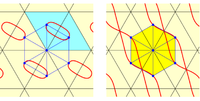
Figure 2. A representation of the fibre $\mu^{-1}(p_{1})$ (left) and $\mu^{-1}(p_{2})$ (right) in $\mathbb{CP}^{2}$ for the points (5.5). The coloured regions are two different fundamental regions for the torus, and the red curves are points a distance $2\pi/3$ from the centre point.

Both diagrams display exactly three distinct points of $\mathbb{CP}^{2}$ in the closure of each coloured fundamental domain, and each of these triples of points forms an equilateral triangle. This can be seen from an inspection of the curves that are the loci of points a distance $2\pi/3$ from the centre point. The latter is correctly separated from each of the other two points, and these two points are correctly separated from each other because distances are translation invariant.

We are now in a position to give a full description of those SIC sets that are orbits of the group generated by (3.5) and (3.6).

Theorem 5.3.

Let $\mathbf{z}=(z_{1},z_{2},z_{3})\in\mathbb{C}^{3}.$ Then $(W\times H)\cdot[\mathbf{z}]$ is a SIC set if and only if one of the variables $z_{1},z_{2},z_{3}$ vanishes, or

(5.6) $$[\mathbf{z}]=\Big{[}\!\cos\theta,\,\omega^{j}\cos(\theta+\hbox{\Large$\frac{2}{3}$}\pi),\,\omega^{k}\cos(\theta+\hbox{\Large$\frac{4}{3}$}\pi)\Big{]},$$

for some $\theta\in[-\frac{1}{2}\pi,\frac{1}{2}\pi)$ and $j,k\in\{0,1,2\}.$

Proof.

Suppose that $\mathbf{z}$ is a unit vector and that $(W\times H)\cdot[\mathbf{z}]$ is a SIC set.

Let $\mathbf{z}^{\prime}=(z_{3},z_{1},z_{2}).$ In the notation (5.1), we have

(5.7) $$|\big{<}\mathbf{z}^{(k)},\mathbf{z}^{\prime}\big{>}|^{2}=\big{|}z_{1}\overline{z}_{3}+\omega^{k}z_{2}\overline{z}_{1}+\omega^{2k}z_{3}\overline{z}_{2}\big{|}^{2}=\beta+2\,\mathrm{Re}\big{[}\omega^{2k}\Delta\big{]},$$

where

(5.8) $$\Delta=z_{1}^{2}\overline{z}_{2}\overline{z}_{3}+z_{2}^{2}\overline{z}_{3}\overline{z}_{1}+z_{3}^{2}\overline{z}_{1}\overline{z}_{2}.$$

By assumption, (5.7) equals $1/4$ for all $k=0,1,2.$ From (5.4) we have $\beta=1/4,$ so the expression in square brackets above must be purely imaginary. This happens for all $k$ if and only if $\Delta=0.$

By assumption, $\mu([\mathbf{z}])\in\mathscr{C},$ so $[\mathbf{z}]$ must lie in a $T$-orbit of $[a,b,c]$ where $a,b,c$ are given by (4.10) for some $\theta.$ Since $a+b+c=0,$ (5.8) and (5.7) tell us that $\mathbf{z}=(a,b,c)$ is a fiducial vector. Let us look for other fiducials in the same $T$-orbit by considering

(5.9) $$(z_{1},z_{2},z_{3})=(a,\,e^{i\beta}b,\,e^{i\gamma}c),$$

having normalized the coefficient of $a.$ Let us assume that $abc\neq 0,$ so $b+c\neq 0.$ Since $\Delta=0,$ we have

(5.10) $$e^{3i\beta}b+e^{3i\gamma}c=b+c.$$

Taking the moduli of both sides gives $\cos(3\beta-3\gamma)=1,$ so $\beta$ equals $\gamma$ mod $2\pi/3.$ It follows that both $\beta$ and $\gamma$ are multiples of $2\pi/3,$ and that $[\mathbf{z}]$ has the form (5.6).

Conversely, the vector (5.6) satisfies (5.7) and projects to $\mathscr{C}.$ Thus its $W\times H$ orbit is a SIC set. ∎

To summarize, any three equally-spaced points on $\mathscr{C}$ form the ‘base’ of a group covariant SIC set. If these are the three midpoints $m_{i}$ of the sides then any point in $\mu^{-1}(m_{i})$ is a fiducial vector. But for a generic point $p\in\mathscr{C},$ the choices are restricted to nine points on the two-torus $\mu^{-1}(p).$ As $p$ approaches a midpoint, these nine points become three.

Remark 5.4.

The methods of this section can be extended to the study of SIC sets in $\mathbb{CP}^{n-1}$ that arise as orbits of $W\times H$ for $n>3.$ Using the moment mapping $\mu\colon\mathbb{CP}^{n-1}\to\mathbb{R}^{n},$ one can define a subset of the simplex $\mu(\mathbb{CP}^{n-1})$ consisting of points whose inverse image contains $H$-orbits of correctly-separated points. For $\mathbb{CP}^{3}$ the relevant subset consists of two circular arcs inside a solid tetrahedron, but is no longer one-dimensional if $n>4,$ as discussed by Lora Lamia NLLD . For applications of the use of $\mu\colon\mathbb{CP}^{3}\to\mathbb{R}^{4}$ in classifying almost-Hermitian structures on manifolds of real dimension six, see Mihaylov Mih .

The SIC sets in $\mathbb{CP}^{2}$ described above have been discussed by Renes et al. RSC , Zhu Zhu , and various other authors. In particular, it is known that any SIC set arising from Theorem 5.3 is isometric to a midpoint solution. This can be proved by adapting the proof of Proposition 6.2 below, but we shall prove a much stronger result in this paper, namely

Theorem 5.5.

Any SIC set $\SS$ in $\mathbb{CP}^{2}$ is congruent modulo $\mathrm{SU}(3)$ to a midpoint solution.

In the next section, we shall work with yet another description of the isometry class of a midpoint solution, in which each circle $C_{i}$ contains exactly two points of the SIC set.

6. Two-point homogeneity

Suppose, going forward, that $\SS$ is a SIC set in $\mathbb{CP}^{2},$ consisting of nine points $[\mathbf{z}_{i}],$ $i=1,\ldots,9.$ Up to the action of the isometry group, we are free to assume that $\SS$ contains the two points of $C_{1}$ represented by the unit vectors

(6.1) $$\textstyle\mathbf{z}_{1}=\hbox{\Large$\frac{1}{\sqrt{2}}$}(0,1,-\omega),\quad\mathbf{z}_{2}=\hbox{\Large$\frac{1}{\sqrt{2}}$}(0,1,-\omega^{2}),$$

which are a distance $2\pi/3$ apart. This is on account of the two-point homogeneity of $\mathbb{CP}^{2}.$ Lemma 3.6 tells us that any other point $[\mathbf{z}]$ of $\SS$ must satisfy

(6.2) $$\big{|}\big{<}\mathbf{z},\mathbf{z}_{j}\big{>}\big{|}^{2}=\hbox{\Large$\frac{1}{4}$}\|\mathbf{z}\|^{2},\qquad j=1,2.$$

Using this equation, we can prove another lemma that emphasizes the important role played by the incircle $\mathscr{C}.$

Lemma 6.1.

The moment map $\mu$ projects any remaining point $[\mathbf{z}]$ of $\SS$ to a point of $\mathscr{C}.$ Indeed, we may take $\mathbf{z}$ to be a unit vector of the form

(6.3) $$\mathbf{z}(\sigma,\phi)=\sqrt{\!\hbox{\Large$\frac{2}{3}$}}\Big{(}\,e^{i\sigma}\cos\phi,\ \cos(\phi+\hbox{\Large$\frac{2}{3}$}\pi),\,\cos(\phi+\hbox{\Large$\frac{4}{3}$}\pi)\,\Big{)}$$

for some $\sigma\in(-\pi,\pi]$ and some $\phi\in(-\frac{1}{2}\pi,\frac{1}{2}\pi].$

To lighten the notation, we shall write $\mathbf{z}[\sigma,\phi]$ as a shorthand for $[\mathbf{z}(\sigma,\phi)],$ so that square brackets on either side of ‘$\mathbf{z}$’ indicate a projective class.

Lemma 4.2 tells us that $\mathbf{z}[\sigma,\phi]$ lies over $\mathscr{C}.$ Observe that $\mu(\mathbf{z}[\sigma,\phi])$ depends only on the angle $\phi$ measured around $\mathscr{C},$ and not on the phase $\sigma.$ Moreover, as $\sigma$ and $\phi$ vary, $\mathbf{z}[\sigma,\phi]$ parametrizes a pinched two-torus, the pinch point being

(6.4) $$\textstyle\mathbf{z}[\sigma,-\frac{1}{2}\pi]=\mathbf{z}[\sigma,\frac{1}{2}\pi]=[0,1,-1],$$

which is evidently independent of $\sigma.$ Having chosen $[\mathbf{z}_{1}],[\mathbf{z}_{2}]$ on $C_{1},$ we can see that any third point of $C_{1}\cap\SS$ must be this point, which explains the pinching. One should note that $\mathbf{z}(\sigma,\phi)=-\mathbf{z}(\sigma,\phi+\pi),$ which is why $\phi=-\pi/2$ is excluded from the non-projective representation (6.3).

Proof of Lemma 6.1.

Let us suppose that $[\mathbf{z}]=[z_{1},z_{2},z_{3}]\in\SS.$ If $z_{2}=0$ then $[\mathbf{z}]\in C_{2}$ and (6.3) will be valid for $\phi=-\pi/6.$ We may therefore take $z_{2}=1$ and set $z_{1}=a,$ $z_{3}=c$ where $a,c\in\mathbb{C}.$ Then by assumption, we have

(6.5) $$|1-c\overline{\omega}|^{2}=|1-c\omega|^{2},$$

which implies that $c$ is real, and

(6.6) $$[\mathbf{z}]=\left[a,\ 1,\ \pm|c|\right].$$

Using (6.2), we see that

(6.7) $$\hbox{\Large$\frac{1}{2}$}(1\pm|c|+|c|^{2})=\hbox{\Large$\frac{1}{4}$}(|a|^{2}+1+|c|^{2}),$$

so $|a|^{2}=(1\pm|c|)^{2},$ and

(6.8) $$|a|^{2}+1+|c|^{2}=2(1\pm|c|+|c|^{2}).$$

Therefore,

(6.9) $$\begin{array}[]{rcl}|a|^{4}+1+|c|^{4}&=&2\pm 4|c|+6|c|^{2}\pm 4|c|^{3}+2|c|^{4}\\[4.0pt] &=&\hbox{\Large$\frac{1}{2}$}(|a|^{2}+1+|c|^{2})^{2}.\end{array}$$

It follows that $\mu$ does indeed map $[\mathbf{z}]$ into $\mathscr{C}.$ In view of Lemma 4.2, we must be able to express $[\mathbf{z}]$ in the stated form for some $e^{i\sigma}\in\mathrm{U}(1).$ ∎

The points $[\mathbf{z}_{1}],[\mathbf{z}_{2}]$ are both fixed by the subgroup $\mathrm{U}(1)$ of (4.1) generated by

(6.10) $$\left(\!\begin{array}[]{ccc}e^{-2ix}&0&0\\ 0&e^{ix}&0\\ 0&0&e^{ix}\end{array}\!\right),$$

so we may assume that a third point of $\SS$ is $\mathbf{z}[0,\theta]$. The next result shows that there does exist a SIC set containing this point for any $\theta.$

Proposition 6.2.

For any $\theta\in[-\frac{1}{2}\pi,\frac{1}{2}\pi),$ the six points

(6.11) $$\begin{array}[]{lll}[0,1,-\omega]=[\mathbf{z}_{1}],&[0,1,-\omega^{2}]=[\mathbf{z}_{2}]&\in C_{1},\\[5.0pt] [1,0,-\omega]=\mathbf{z}[-\frac{2}{3}\pi,\!-\frac{1}{6}\pi],&[1,0,-\omega^{2}]=\mathbf{z}[\frac{2}{3}\pi,\!-\frac{1}{6}\pi]&\in C_{2},\\[5.0pt] [1,-\omega,0]=\mathbf{z}[-\frac{2}{3}\pi,\frac{1}{6}\pi],&[1,-\omega^{2},0]=\mathbf{z}[\frac{2}{3}\pi,\frac{1}{6}\pi]&\in C_{3},\end{array}$$

combine with three points

(6.12) $$\textstyle\mathbf{z}[0,\theta-\frac{1}{3}\pi],\qquad\mathbf{z}[0,\theta],\qquad\mathbf{z}[0,\theta+\frac{1}{3}\pi]$$

to form a SIC set isometric to a midpoint solution.

We shall denote this SIC set by $\mathbb{S}_{\theta};$ it is illustrated in Figure 3.

Proof.

Consider the matrix

(6.13) $$M=\frac{1}{\sqrt{3}}\!\left(\begin{array}[]{ccc}\omega^{2}&\omega&1\\ 1&\omega&\omega^{2}\\ 1&1&1\end{array}\right).$$

It is easy to check that $M\in\mathrm{U}(3)$ and that $M^{3}=i\omega^{2}I.$ A calculation shows that

(6.14) $$\textstyle M\kern 1.0pt\mathbf{z}(0,\theta)^{\!\top}=\hbox{\Large$\frac{1}{\sqrt{2}}$}\!\left(e^{i\theta}\omega^{2},\ e^{-i\theta},\ 0\right)^{\!\top},$$

so that $M$ maps $\mathbf{z}[0,\theta]$ to the point $[e^{2i\theta},\,\omega,\,0]$ of $C_{3}.$ Moreover, $M$ maps the array (6.11) to the array

(6.15) $$\begin{array}[]{ll}[0,1,-1],&[1,0,-\omega],\\[5.0pt] [1,0,-\omega^{2}],&[0,1,-\omega^{2}],\\[5.0pt] [0,1,-\omega],&[1,0,-1]\end{array}$$

of points in $C_{1}\sqcup\,C_{2}.$ It follows that $M$ maps $\mathbb{S}_{\theta}$ onto three triples of points, each triple belonging to $C_{i}$ for some $i=1,2,3.$ ∎

The first six points (6.11) of $\mathbb{S}_{\theta}$ do not depend on $\theta,$ whereas the last triple of points can be rotated at will (by varying $\theta$) around a circle $C_{3}^{\prime}$ covering $\mathscr{C}$. For example, $\mathbf{z}[0,0]$ lies over the point $p_{1}$ of $\mathscr{C}$ diametrically opposite $m_{1}$ (see (5.5)).

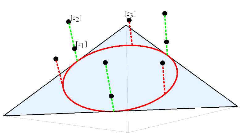
Figure 3. The SIC set $\mathbb{S}_{\theta}$ defined by Proposition 6.2 contains two points in each circle $C_{i}$ (including $[\mathbf{z}_{1}],[\mathbf{z}_{2}]$ in $C_{1}$) that do not depend on $\theta,$ together with a triple of points (including $[\mathbf{z}_{3}]$) that $\mu$ also projects to $\mathscr{C}$ for which $\theta$ represents the angle around $\mathscr{C}.$

Remark 6.3.

Nine points in $\mathbb{CP}^{2}$ are the inflection points of a non-singular cubic curve if and only if the line determined by any two of them contains a third. This being the case, there are twelve such lines altogether, on which the nine points lie by threes, with four of the twelve lines through each of the nine points, thus forming the so-called Hesse configuration $\{9_{4},12_{3}\}$. For the points of $\mathbb{S}_{\theta}$ to arise in this way, and as described by Hughston Hugh and Dang et al. DBBA , the projective line $\mathbb{L}_{1}\cong\mathbb{CP}^{1}$ generated $[\mathbf{z}_{1}],[\mathbf{z}_{2}]$ must contain a third point of $\mathbb{S}_{\theta}.$ But $\mathbb{L}_{1}$ is the inverse image by $\mu$ of the side of $\mathscr{T}$ containing $m_{1},$ and will only contain another point if $\theta$ assumes one of the values $\pm\pi/2,\pm\pi/6.$ This occurs when the three red legs (the ones generated by $[\mathbf{z}_{3}]$ by rotation by $2\pi/3$) in Figure 3 line up with the green legs (the ones over the midpoints), and $\mathbb{S}_{\theta}$ is then itself a special midpoint solution.

Example 6.4.

The unitary transformation $M$ maps $C_{3}^{\prime}$ to $C_{3}.$ It permutes the elements of the SIC set $(W\times H)\cdot[0,1,-1],$ though it fixes none of them. The matrices

(6.16) $$A=\left(\!\begin{array}[]{ccc}0&1&0\\ 0&0&1\\ 1&0&0\end{array}\!\right),\quad B=\left(\!\begin{array}[]{ccc}1&0&0\\ 0&\omega&0\\ 0&0&\omega^{2}\end{array}\!\right)$$

generate $W$ and $H$ respectively, and satisfy

(6.17) $$M\kern-1.0ptAM^{-1}=\omega B,\qquad M\kern-1.0ptBM^{-1}=\omega^{2}A^{-1}B^{-1}.$$

It follows that $M$ is an element of the so-called Clifford group, the normalizer of $W\times H$ in $\mathrm{U}(3).$ Modulo phase, this normalizer is isomorphic to a semidirect product $\mathrm{SL}(2,\mathbb{Z}_{3})\ltimes(\mathbb{Z}_{3})^{2}$ (see Appleby App and Horrocks-Mumford HM ). Equation (6.17) asserts that $M$ induces the automorphism of $W\times H$ given by

(6.18) $$\left(\!\begin{array}[]{cc}0&-1\\ 1&-1\end{array}\!\right)\in\mathrm{SL}(2,\mathbb{Z}_{3}).$$

It is conjectured that a fiducial vector can always be found in an eigenspace of some element of the Clifford group (see Zauner Z ). In the case of $M,$ a computation shows that any one of its eigenvectors defines a point of $\mathbb{CP}^{2}$ whose orbit under $W\times H$ is a configuration of nine points arranged in nine lines. Each of the 27 pairs of points lying on one of the nine lines has a cross ratio $\kappa=1/3,$ whereas the remaining nine pairs of points have $\kappa=0.$ Compared to the Hesse configuration above, this means that three of the twelve triples of points are not collinear, but each of these three triples forms an orthonormal basis of $\mathbb{C}^{3}.$

Remark 6.5.

If an isometry is to fix both $[\mathbf{z}_{1}]$ and $[\mathbf{z}_{2}],$ there is no ambiguity remaining in the choice of $\phi\in[\!-\!\pi/2,\pi/2)$ in Lemma 6.1. However, we are at liberty to interchange $[\mathbf{z}_{1}]$ and $[\mathbf{z}_{2}]$ by applying either complex conjugation or the unitary

(6.19) $$\left(\!\begin{array}[]{ccc}1&0&0\\ 0&0&1\\ 0&1&0\end{array}\!\right).$$

The former has the effect of replacing $\sigma$ by $-\sigma,$ and the latter of replacing $\phi$ by $-\phi$ in (6.3). In particular, the congruence class of the unordered set $\mathbb{S}_{\theta}$ uniquely specifies $|\theta|.$ This fact can also be verified using a triple product that measures the signed area of the planar geodesic triangle spanned by three points. See, for example, Brody and Hughston BH and references cited therein.

7. Trigonometry

From now on, we shall assume that $\SS$ is a SIC set in $\mathbb{CP}^{2}$ that contains the points $[\mathbf{z}_{1}],[\mathbf{z}_{2}]$ defined by (6.1). Lemma 6.1 tells that any other point of $\SS$ has the form

(7.1) $$\mathbf{z}[\sigma,\phi]=\Big{[}\,e^{i\sigma}\cos\phi,\ \cos(\phi+\hbox{\Large$\frac{2}{3}$}\pi),\,\cos(\phi+\hbox{\Large$\frac{4}{3}$}\pi)\omega^{2}\,\Big{]},$$

where $(\sigma,\phi)$ belongs to the rectangle

(7.2) $$\mathscr{R}=(-\pi,\pi]\times(-\hbox{\Large$\frac{1}{2}$}\pi,\hbox{\Large$\frac{1}{2}$}\pi].$$

The next result, from which many others follow, translates distance into the new ‘rectangular’ coordinates.

Lemma 7.1.

Suppose that $\phi,\psi\in(-\frac{1}{2}\pi,\frac{1}{2}\pi)\setminus\{-\frac{1}{6}\pi,\frac{1}{6}\pi\}.$ Then the points $\mathbf{z}[\sigma,\phi]$ and $\mathbf{z}[\tau,\psi]$ are the correct distance $2\pi/3$ apart if and only if

(7.3) $$1-\cos(\sigma-\tau)=\frac{9(1+2\cos(2(\phi-\psi)))\sec\phi\sec\psi}{16(\cos\phi\cos\psi+3\sin\phi\sin\psi)}.$$

Proof.

Not only do we have to establish the formula, but we also need to show that the assumptions imply that the denominator of the fraction is non-zero. We use the abbreviated notation

(7.4) $$\begin{array}[]{rcl}\Gamma_{0}&=&\cos\phi\cos\psi,\\[4.0pt] \Gamma_{1}&=&\cos(\phi+\frac{2}{3}\pi)\cos(\psi+\frac{2}{3}\pi),\\[4.0pt] \Gamma_{2}&=&\cos(\phi+\frac{4}{3}\pi)\cos(\psi+\frac{4}{3}\pi).\end{array}$$

The condition on the cross ratio for correct separation is that

(7.5) $$\hbox{\Large$\frac{4}{9}$}\big{|}e^{i(\sigma-\tau)}\Gamma_{0}+\Gamma_{1}+\Gamma_{2}\big{|}^{2}=\hbox{\Large$\frac{1}{4}$},$$

which gives

(7.6) $$2\cos(\sigma-\tau)\Gamma_{0}(\Gamma_{1}+\Gamma_{2})+\Gamma_{0}^{2}+(\Gamma_{1}+\Gamma_{2})^{2}=\hbox{\Large$\frac{9}{16}$},$$

and therefore

(7.7) $$32\Gamma_{0}(\Gamma_{1}+\Gamma_{2})(1-\cos(\sigma-\tau))=32\Gamma_{0}(\Gamma_{1}+\Gamma_{2})+16\Gamma_{0}^{2}+16(\Gamma_{1}+\Gamma_{2})^{2}-9.$$

A calculation shows that the right-hand side of (7.7) is equal to

(7.8) $$9(1+2\cos(2(\phi-\psi))),$$

which vanishes when $\cos(\phi-\psi)=\pm 1/2.$ By hypothesis, $\Gamma_{0}\neq 0.$ If

(7.9) $$\Gamma_{1}+\Gamma_{2}=\hbox{\Large$\frac{1}{2}$}[\cos\phi\cos\psi+3\sin\phi\sin\psi]$$

vanishes, then

(7.10) $$\cos\phi\cos\psi+\sin\phi\sin\psi=\cos(\phi-\psi)=\pm\hbox{\Large$\frac{1}{2}$},$$

and hence

(7.11) $$\cos\phi\cos\psi=\pm\hbox{\Large$\frac{3}{4}$},\quad\sin\phi\sin\psi=\mp\hbox{\Large$\frac{1}{4}$}.$$

Now set $x=\tan\phi$ and $y=\tan\psi.$ Then $xy=-1/3$ and it holds that

(7.12) $$\pm\sqrt{3}=\tan(\phi-\psi)=\frac{x-y}{1+xy}=\hbox{\Large$\frac{3}{2}$}(x-y).$$

We therefore have

(7.13) $$(x+y)^{2}=(x-y)^{2}+4xy=0,$$

and $\phi=-\psi=\pm\pi/6,$ values that are excluded. We may therefore assume that $\Gamma_{0}(\Gamma_{1}+\Gamma_{2})\neq 0,$ and (7.3) follows. ∎

Lemma 7.2.

If $\SS$ contains the pinch point $[0,1,-1]$ as well as $[0,1,-\omega]$ and $[0,1,-\omega^{2}],$ then $\SS$ is a midpoint solution.

Proof.

By hypothesis, $\SS$ contains three points of the circle $C_{1}.$ If $\mathbf{z}[\sigma,\phi]$ is a fourth point of $\SS,$ then (7.1) is correctly separated from $[0,1,-1]$ and

(7.14) $$\cos(\phi+\hbox{\Large$\frac{2}{3}$}\pi)-\cos(\phi+\hbox{\Large$\frac{4}{3}$}\pi)=\pm\hbox{\Large$\frac{\sqrt{3}}{2}$}.$$

This implies that $\sin\phi=\pm 1/2,$ and forces $\mathbf{z}[\sigma,\phi]$ to lie on $C_{2}\sqcup C_{3}.$ Therefore $\SS$ lies in the disjoint union $C_{1}\sqcup C_{2}\sqcup C_{3}.$ ∎

One can rewrite (7.3) as

(7.15) $$\begin{array}[]{rcl}\cos(\sigma-\tau)&=&\displaystyle 1-\frac{9(1+2\cos 2(\phi-\psi))}{4(4\cos^{2}\phi\cos^{2}\psi+3\sin 2\phi\sin 2\psi)}\\[15.0pt] &=&\displaystyle\frac{-5+4\cos 2\phi+4\cos 2\psi-14\cos 2\phi\cos 2\psi-6\sin 2\phi\sin 2\psi}{4(1+\cos 2\phi+\cos 2\psi+\cos 2\phi\cos 2\psi+3\sin 2\phi\sin 2\psi)}.\end{array}$$

We shall convert the right-hand side into a rational function by setting

(7.16) $$x=\tan\phi,\quad y=\tan\psi.$$

In the light of Lemma 7.2, we assume from now on that $x,y$ are finite.

Equation (7.15) simplifies to

(7.17) $$\cos(\sigma-\tau)=\frac{-11+9x^{2}+9y^{2}-27x^{2}y^{2}-24xy}{16(1+3xy)}.$$

If $1+3xy=0,$ then the numerator on top of it must also vanish, so $x^{2}+y^{2}=2/3$ and $(x+y)^{2}=0.$ Thus (as in the previous proof) $x=-y=\pm 1/\kern-2.0pt\sqrt{3}.$ This means that $\mathbf{z}[\sigma,\phi]$ lies on one of the circles $C_{2},C_{3},$ and $\mathbf{z}[\tau,\psi]$ lies on the other, so there are no restrictions on $\sigma$ and $\tau.$

The main result of this section is the following, which establishes a criterion for the existence in $\mathbb{CP}^{2}$ of five points that are correctly separated from one another.

Theorem 7.3.

Suppose that $\mathbf{z}[\sigma,\phi],\mathbf{z}[\tau,\psi],\mathbf{z}[\upsilon,\chi]$ are three points of $\mathbb{CP}^{2},$ a distance $2\pi/3$ away from each other (and from $[\mathbf{z}_{1}],[\mathbf{z}_{2}]$). Set $p=x+y+z,$ $q=yz+zx+xy,$ $r=xyz,$ where $x=\tan\phi,$ $y=\tan\psi,$ $z=\tan\chi.$ Then $F(p,q,r)=0$ where

(7.18) $$\begin{array}[]{c}F(p,q,r)=9-22p^{2}+9p^{4}+87q-126p^{2}q+27p^{4}q+298q^{2}-226p^{2}q^{2}\\ +24p^{4}q^{2}+414q^{3}-138p^{2}q^{3}+189q^{4}+27q^{5}-3pr-50p^{3}r-15p^{5}r\\ +88pqr-48p^{3}qr+234pq^{2}r+18p^{3}q^{2}r-144pq^{3}r+81pq^{4}r+189r^{2}\\ -480p^{2}r^{2}-153p^{4}r^{2}+1398qr^{2}-306p^{2}qr^{2}+2736q^{2}r^{2}-486p^{2}q^{2}r^{2}\\ +810q^{3}r^{2}+243q^{4}r^{2}-558pr^{3}-486p^{3}r^{3}+2376pqr^{3}-810pq^{2}r^{3}\\ +567r^{4}-162p^{2}r^{4}+6399qr^{4}+486q^{2}r^{4}+1701pr^{5}+2187r^{6}.\end{array}$$

Proof.

Although (7.18) is rather complicated, the existence of such an expression is a consequence of the elementary trigonometric identity

(7.19) $$A+B+C=0\ \Rightarrow\ \cos^{2}\!A+\cos^{2}\!B+\cos^{2}\!C=1+2\cos A\cos B\cos C,$$

which is tailor made for (7.17). The identity itself can be proved by writing applying more standard ones to the sum $A+(B+C).$ Denote the right-hand side of (7.17) by the symmetric function $c(x,y).$ Then

(7.20) $$c(x,y)^{2}+c(y,z)^{2}+c(z,x)^{2}=1+2c(x,y)c(y,z)c(z,x).$$

This simplifes into the vanishing of the quotient

(7.21) $$\frac{243\,f(x,y,z)}{2048(1+3xy)^{2}(1+3yz)^{2}(1+3zx)^{2}},$$

in which $f$ is a totally symmetric polynomial. We can then use the Mathematica command $\mathtt{SymmetricReduction}$ to express

(7.22) $$f(x,y,z)=F(p,q,r)$$

as a function of the elementary symmetric polynomials, and the result follows. ∎

8. Graphical interpretation

Suppose once again that $\SS$ is a SIC set in $\mathbb{CP}^{2}$ containing $[\mathbf{z}_{1}]=[0,1,-\omega]$ and $[\mathbf{z}_{2}]=[0,1,-\omega^{2}],$ and (in view of Lemma 7.2) not the third point $[0,1,-1]$ of $C_{1}.$ The planar parametrization (7.3) of the remaining points of $\SS$ enables us to describe graphically the quest for such SIC sets. Before we do this, we prove two results that help with their classification.

Setting $\phi=-\pi/6$ in (6.3) defines the circle $C_{2},$ and $\phi=\pi/6$ the circle $C_{3}.$ It will be convenient to consider three more circles $C_{-},C_{0},C_{+}$ given by $\sigma=-2\pi/3$, $0$, $2\pi/3$ respectively. Unlike $C_{1},C_{2},C_{3},$ these three are not disjoint: they meet in $[0,1,-1].$ The circles $C_{2},C_{3}$ are represented by horizontal lines in $\mathscr{R},$ and $C_{-},C_{0},C_{+}$ by equally-spaced vertical lines; all five have diameter $\pi.$ The lines representing $C_{-},C_{0}$ and $C_{2}$ are visible in Figure 7.

Lemma 8.1.

If $\SS$ contains a point $\mathbf{z}[\sigma,\phi]$ with $|\phi|=\pi/6$ then $\SS$ is isometric to a midpoint solution.

Proof.

We can use the isometry (6.10) to shift all points of $\SS$ by a translation parallel to the horizontal axis within our rectangle $\mathscr{R}.$ We may therefore assume that $\sigma=0.$ Suppose for definiteness that $\phi=\pi/6,$ so that $x=1/\kern-2.0pt\sqrt{3}$ and $\mathbf{z}[\sigma,\phi]\in C_{3}.$ Suppose that $\mathbf{z}[\tau,\psi]$ is a fourth point of $\SS,$ and apply (7.17). The numerator equals

(8.1) $$-11+9x^{2}+9y^{2}-27x^{2}y^{2}-24xy=-8(1+\sqrt{3}y),$$

and the right-hand side of (7.17) becomes $-1/2$ unless $y=-1/\kern-2.0pt\sqrt{3}.$ It follows that $\tau=\pm 2\pi/3$ or $\psi=-\pi/6.$ Indeed, the set of points correctly separated from $[\mathbf{z}_{1}],$ $[\mathbf{z}_{2}]$ and $\mathbf{z}[0,\pi/6]$ is the union $C_{-}\cup C_{2}\cup C_{+}.$ This union must now contain six points of $\SS,$ and no circle can contain more than three.

Now suppose that $\SS$ contains distinct points $\mathbf{z}[\frac{2}{3}\pi,\psi]\in C_{+}$ and $\mathbf{z}[\upsilon,-\frac{1}{6}\pi]\in C_{2}$. Then (7.17) tells us that either $y=1/\kern-2.0pt\sqrt{3}$ (and so $\psi=\pi/6$), or else

(8.2) $$\textstyle\cos(\frac{2}{3}\pi-\upsilon)=-\frac{1}{2}$$

and $\upsilon=-2\pi/3$ or $\upsilon=0$. So either the first point lies on $C_{3}$, or else the second point lies on $C_{-}\sqcup C_{0}$. Now suppose that $\SS$ contains $\mathbf{z}[-\frac{2}{3}\pi,\psi]\in C_{-}$ and $\mathbf{z}[\frac{2}{3}\pi,\chi]\in C_{+}$ This time, (7.17) yields

(8.3) $$(3y^{2}-1)(3z^{2}-1)=0,$$

and at least one of the two points is one of the last four in (6.11). We may also suppose that $[0,1,-1]\not\in\SS$ by Lemma 7.2. It then follows that $\SS$ consists of $[\mathbf{z}_{1}]$ and $[\mathbf{z}_{2}]$, the two points in $C_{-}\cap(C_{2}\sqcup C_{3}),$ the two points in $C_{0}\cap(C_{2}\sqcup C_{3})$ and three points in $C_{+},$ or the same thing with $C_{-}$ and $C_{+}$ interchanged. Applying (6.10) with $x=\pm 2\pi/3,$ we obtain exactly the SIC set $\mathbb{S}_{\theta}$ for some $\theta$ (like the one that includes the green points in Figures 6 and 7). Then the result follows from Proposition 6.2. ∎

Lemma 8.2.

Suppose that $\SS$ is a SIC set that contains $[\mathbf{z}_{1}],[\mathbf{z}_{2}]$ and $\mathbf{z}[0,\theta].$ Recall that any SIC set has this property up to isometry. If $\SS$ contains distinct points $\mathbf{z}[\sigma_{1},\phi],\mathbf{z}[\sigma_{2},\phi]$ with $\sigma_{1},\sigma_{2}\in(-\pi,\pi)$ then it is isometric to a midpoint solution.

Proof.

First observe that $\sigma_{1}+\sigma_{2}=0;$ this follows by applying Lemma 7.1 in which we can set $(\tau,\psi)=(0,\theta)$ to obtain $\cos\sigma_{1}=\cos\sigma_{2}.$ So take $\sigma=\sigma_{1}.$

In view of Lemma 8.1, we may suppose that $x=\tan\phi$ is different from $\pm 1/\kern-2.0pt\sqrt{3}.$ We can choose a sixth point $\mathbf{z}[\tau,\psi]$ of $\SS$ such that $\tau\neq\pi,$ since the circle $\tau=\pi$ can contain at most three points a distance $2\pi/3$ apart. It follows from (7.17) that either $1+3xy=0$ (and we can apply Lemma 8.1) or

(8.4) $$\cos(\sigma-\tau)=\cos(-\sigma-\tau).$$

Since $\sigma=0$ and $\sigma=\pi$ do not yield distinct points, the only possibility remaining from our assumption is that $\tau=0.$ If $t=\tan\theta$ and $y=\tan\psi$, (7.17) implies that

(8.5) $$t^{2}+y^{2}-3t^{2}y^{2}-8ty-3=0.$$

This gives

(8.6) $$y=\frac{t\pm\sqrt{3}}{1\mp\sqrt{3}\,t},$$

$\psi=\theta\pm\pi/3$ modulo $\pi.$ This is the configuration of three points visible on the central vertical axis in Figure 7. All together, $\SS$ now contains at most seven points including $[\mathbf{z}_{1}]$ and $[\mathbf{z}_{2}],$ which is a contradiction. Using (7.17), one can in fact show that given the sixth point, either $\phi$ or $\psi$ must equal $\pm\pi/6.$ ∎

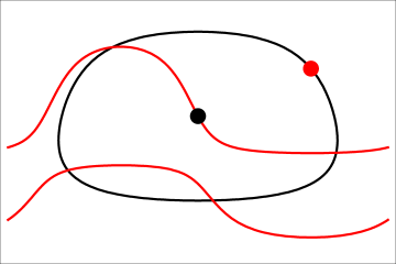
Figure 4. The black (resp., red) point is correctly separated from all points on the black (resp., red) curve. The two points cannot belong to a SIC set because there are only four remaining points correctly separated from them both.

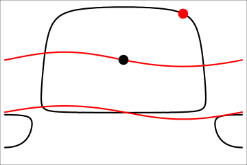
Figure 5. The points that are correctly separated from the black point can form a disconnected set. Here, there appear to be five points correctly separated from the red and black points, but these five points do not in fact form part of a SIC set.

We are now in a position to illustrate the problem of finding SIC sets that contain $[\mathbf{z}_{1}]$ and $[\mathbf{z}_{2}].$ We can (and shall) assume that a third point of $\SS$ is $\mathbf{z}[0,\theta]$ for some fixed $\theta\in(-\pi/2,\pi/2).$ This point corresponds to one on the central vertical axis of the rectangle $\mathscr{R},$ and will be displayed by a black dot in the figures. We shall draw some curves to illustrate the concept of correctly separated points in $\mathscr{R},$ meaning that the distance between the points they represent in $\mathbb{CP}^{2}$ equals $2\pi/3.$ A fourth point $\mathbf{z}[\sigma,\phi]$ of $\SS$ will be displayed by a red dot.

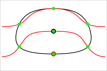
Figure 6. Here the fourth point $\mathbf{z}[0,\frac{1}{16}\pi-\frac{1}{3}\pi]$ belongs to $\mathbb{S}_{\theta}$ which is generated by the remaining five points on the intersection of the black and red curves.

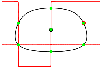
Figure 7. Here the fourth point $\mathbf{z}[\frac{2}{3}\pi,\frac{1}{6}\pi]\in\mathbb{S}_{\theta}$ is equidistant from all points on the circles $C_{-},C_{0},C_{2}$, represented by straight lines in $\mathscr{R}.$ The segments top and bottom collapse to the pinch point.

In Figure 4, $\theta=\pi/16$ so that the third point $\mathbf{z}[0,\theta]$ of $\SS$ is close to centre of $\mathscr{R}.$ The black curve is the set of points $\mathbf{z}[\sigma,\phi]$ which are a distance $2\pi/3$ from $\mathbf{z}[0,\theta].$ The remaining six points of $\SS$ must therefore lie on this curve. One such example is represented by the red dot, which actually has $\phi=\pi/4.$ Points $\mathbf{z}[\tau,\psi]$ a distance $2\pi/3$ apart from this red point are those on the red curve (which has two components). The intersection of the black and red curves consists of points which are correctly separated from both the third and fourth points. Since there are only four of these (we require five), the value $x=\tan\phi=1$ cannot in fact occur when $\theta=\pi/16.$

The nature of the black curve is heavily dependent on the value chosen of $\theta$ and $t=\tan\theta.$ If $\mathbf{z}[\pi,\phi]$ is correctly separated from $\mathbf{z}[0,\theta]$ and $x=\tan\phi$ then

(8.7) $$9(1-3t^{2})x^{2}+24tx+9t^{2}+5=0.$$

Computing the roots of the discriminant as a function of $t,$ (8.7) has distinct roots if and only if $|t|>\sqrt{5/27}=0.430\ldots$ In this case, the black curve has two connected components, and an example is visible in Figure 5 for which $\theta=\pi/7.$ This time the red point $(\sigma,\phi)$ is chosen (with $x$ approximately $4.75$) so that there are exactly five points correctly separated from both the (black and red) third and fourth points. Subsequent analysis will show that these five points are not correctly separated from each other.

Although the fourth (red) point in Figure 4 is not admissible (nor, in fact, is that in Figure 5), Proposition 6.2 implies that there does exists a SIC set, namely $\mathbb{S}_{\theta},$ containing the first three points, so there must be at least six points on the black curve that are admissible. For Figures 6 and 7, we return to the value $\theta=\pi/16,$ and display these six points in green.

In Figure 6, we have chosen the fourth point $\mathbf{z}[\sigma,\phi]$ to be the admissible one with $\sigma=0$ and $\phi$ negative. In Figure 7, we have chosen the fourth point to be one of the points of $\mathbb{S}_{\theta}$ that does not depend on $\theta.$ Recall that the top and bottom boundary of $\mathscr{R}$ is a single point, and that the horizontal lines $\phi=\pm\pi/6$ are the circles $C_{2},C_{3}.$ Figure 7 illustrates the fact that any point of $C_{2}$ is correctly separated from $[\mathbf{z}_{1}],$ $[\mathbf{z}_{2}]$ and a given point of $C_{3},$ as we explained in the proof of Lemma 8.1.

9. Symmetrization

We suppose now that $\SS$ is a SIC set containing, in addition to $[\mathbf{z}_{1}]=[0,1,-\omega]$ and $[\mathbf{z}_{2}]=[0,1,-\omega^{2}],$ four more points $\mathbf{z}[\sigma_{i},\phi_{i}],$ $i=3,4,5,6,$ with $t=\phi_{3},$ $x=\phi_{4},$ $y=\phi_{5},$ $z=\phi_{6}.$

In view of Theorem 7.3 and equation (7.21), our task is to investigate the system of polynomial equations given by

(9.1) $$f(x,y,z)=0,\ \ f(t,y,z)=0,\ \ f(t,x,z)=0,\ \ f(t,x,y)=0.$$

Since $f$ is itself symmetric, the whole system is invariant under the action of the group of permutations of $t,x,y,z.$ There are refinements of Buchberger’s algorithm for dealing with symmetric ideals, but we shall adopt the technique outlined in St . Namely, we shall convert the system into a system four equations, each of which involves only the elementary symmetric polynomials defined by

(9.2) $$\begin{array}[]{l}a=t+x+y+z,\\ b=tx+ty+tz+yz+zx+xy,\\ c=xyz+tyz+txz+txy,\\ d=txyz.\end{array}$$

To accomplish this, first define

(9.3) $$F_{1}=f(x,y,z)+f(t,y,z)+f(t,x,z)+f(t,x,y),$$

and consider

(9.4) $$g(t,x,y,z)=\frac{f(t,x,y)-f(t,x,z)}{y-z}.$$

This is a polynomial in $t,x,y,z,$ so we can symmetrize it to get

(9.5) $$\begin{array}[]{r}F_{2}=g(t,x,y,z)+g(t,y,z,x)+g(t,z,x,y)\\ +g(x,y,t,z)+g(x,z,t,y)+g(y,z,x,t).\end{array}$$

Next, set

(9.6) $$h(t,x,y,z)=\frac{g(t,x,y,z)-g(t,y,x,z)}{x-y},$$

so as to define

(9.7) $$\begin{array}[]{r}F_{3}=h(t,x,y,z)+h(t,y,z,x)+h(t,z,x,y)\\ +h(x,y,t,z)+h(x,z,t,y)+h(y,x,t,z)\\ +h(z,x,y,t)+h(x,y,z,t)+h(y,z,x,t)\\ +h(z,y,t,x)+h(y,z,t,x)+h(z,x,t,y),\\[10.0pt] \displaystyle F_{4}=\frac{h(t,x,y,z)-h(x,t,y,z)}{t-x}.\phantom{oooooo}\end{array}$$

Each of $F_{1},F_{2},F_{3},F_{4}$ is a symmetric polynomial in $t,x,y,z,$ and can therefore be expressed as a polynomial in $a,b,c,d.$ The proof of Theorem 5.5 proceeds by examination of the system

(9.8) $$F_{1}(a,b,c,d)=0,\ \ F_{2}(a,b,c,d)=0,\ \ F_{3}(a,b,c,d)=0,\ \ F_{4}(a,b,c,d)=0.$$

To determine the polynomials $F_{i}$ in practice, we used again the Mathematica command $\mathtt{SymmetricReduction}$. For completeness we list them explicitly:

$$\begin{array}[]{l}F_{1}=36-66a^{2}+27a^{4}+218b-288a^{2}b+54a^{4}b+614b^{2}-452a^{2}b^{2}+48a^{4}b^{2}+828b^{3}-276a^{2}b^{3}\\[-0.7pt] +378b^{4}+54b^{5}-41ac+159a^{3}c-63a^{5}c-567abc+270a^{3}bc-246ab^{2}c+18a^{3}b^{2}c-279ab^{3}c\\[-0.7pt] +81ab^{4}c+834c^{2}-708a^{2}c^{2}-153a^{4}c^{2}+1968bc^{2}-171a^{2}bc^{2}+2871b^{2}c^{2}-486a^{2}b^{2}c^{2}+810b^{3}c^{2}\\[-0.7pt] +243b^{4}c^{2}-693ac^{3}-486a^{3}c^{3}+2376abc^{3}-810ab^{2}c^{3}+567c^{4}-162a^{2}c^{4}+6399bc^{4}+486b^{2}c^{4}\\[-0.7pt] +1701ac^{5}+2187c^{6}-712d+687a^{2}d+414a^{4}d-2632bd+351a^{2}bd+216a^{4}bd-4470b^{2}d+1107a^{2}b^{2}d\\[-0.7pt] -5454b^{3}d+243a^{2}b^{3}d-1782b^{4}d-486b^{5}d+453acd+927a^{3}cd-3330abcd+2835a^{3}bcd-7857ab^{2}cd\\[-0.7pt] +1458ab^{3}cd+666c^{2}d-1485a^{2}c^{2}d-4968bc^{2}d+2268a^{2}bc^{2}d-24786b^{2}c^{2}d-1944b^{3}c^{2}d-6075ac^{3}d\\[-0.7pt] -9477abc^{3}d-1701c^{4}d-13122bc^{4}d+4656d^{2}-531a^{2}d^{2}-2673a^{4}d^{2}+14436bd^{2}+9774a^{2}bd^{2}+12042b^{2}d^{2}\\[-0.7pt] -2349a^{2}b^{2}d^{2}+13608b^{3}d^{2}+972b^{4}d^{2}+3861acd^{2}-1944a^{3}cd^{2}+37665abcd^{2}+13365ab^{2}cd^{2}+6966c^{2}d^{2}\\[-0.7pt] +8991a^{2}c^{2}d^{2}+7776bc^{2}d^{2}+19683b^{2}c^{2}d^{2}+13122ac^{3}d^{2}-11448d^{3}-11907a^{2}d^{3}-35640bd^{3}-12393a^{2}bd^{3}\\[-0.7pt] -7290b^{2}d^{3}-4374b^{3}d^{3}-16281acd^{3}-26244abcd^{3}-13122c^{2}d^{3}+8748d^{4}+6561a^{2}d^{4}+13122bd^{4}.\end{array}$$

$$\begin{array}[]{l}F_{2}=63a-243a^{3}+81a^{5}+829ab-846a^{3}b+81a^{5}b+1706ab^{2}-642a^{3}b^{2}+1092ab^{3}+18a^{3}b^{3}+45ab^{4}\\[-0.7pt] +81ab^{5}-1086c+741a^{2}c-18a^{4}c-2348bc+123a^{2}bc-153a^{4}bc+24b^{2}c-630a^{2}b^{2}c+2493b^{3}c\\[-0.7pt] -486a^{2}b^{3}c+810b^{4}c+243b^{5}c+135ac^{2}+81a^{3}c^{2}-18abc^{2}-486a^{3}bc^{2}+2376ab^{2}c^{2}-810ab^{3}c^{2}\\[-0.7pt] -162c^{3}+567bc^{3}-162a^{2}bc^{3}+6399b^{2}c^{3}+486b^{3}c^{3}+1701abc^{4}+2187bc^{5}-1512ad+2583a^{3}d\\[-0.7pt] +405a^{5}d-8709abd+2232a^{3}bd-11583ab^{2}d+1944a^{3}b^{2}d-7479ab^{3}d-891ab^{4}d+1926cd+1080a^{2}cd\\[-0.7pt] +1701a^{4}cd+270bcd-5859a^{2}bcd-2862b^{2}cd+4374a^{2}b^{2}cd-11988b^{3}cd-972b^{4}cd-2916ac^{2}d\\[-0.7pt] +486a^{3}c^{2}d-25272abc^{2}d-7533ab^{2}c^{2}d-5103a^{2}c^{3}d-1701bc^{3}d-8748b^{2}c^{3}d-6561ac^{4}d+10422ad^{2}\\[-0.7pt] -3807a^{3}d^{2}+37071abd^{2}-3888a^{3}bd^{2}+29160ab^{2}d^{2}+4617ab^{3}d^{2}+486cd^{2}+14337a^{2}cd^{2}+41472bcd^{2}\\[-0.7pt] +17010a^{2}bcd^{2}+7290b^{2}cd^{2}+6561b^{3}cd^{2}+15309ac^{2}d^{2}+26244abc^{2}d^{2}+13122c^{3}d^{2}-46656ad^{3}\\[-0.7pt] -6561a^{3}d^{3}-28431abd^{3}-10935ab^{2}d^{3}-10206cd^{3}-13122a^{2}cd^{3}-30618bcd^{3}+19683ad^{4}.\end{array}$$

$$\begin{array}[]{l}F_{3}=780-978a^{2}-180a^{4}+27a^{6}+3468b-1320a^{2}b-396a^{4}b+4968b^{2}-81a^{2}b^{2}+54a^{4}b^{2}+2268b^{3}\\[-0.7pt] -108a^{2}b^{3}+324b^{4}+243a^{2}b^{4}-594ac-693a^{3}c-459a^{5}c+2250abc-1161a^{3}bc+6993ab^{2}c-1458a^{3}b^{2}c\\[-0.7pt] +2430ab^{3}c+729ab^{4}c+900c^{2}-1188a^{2}c^{2}-1458a^{4}c^{2}+648bc^{2}+7128a^{2}bc^{2}-2430a^{2}b^{2}c^{2}+1701ac^{3}\\[-0.7pt] -486a^{3}c^{3}+19197abc^{3}+1458ab^{2}c^{3}+5103a^{2}c^{4}+6561ac^{5}-5304d+4446a^{2}d+4509a^{4}d-22644bd\\[-0.7pt] -6318a^{2}bd+3645a^{4}bd-32076b^{2}d-10044a^{2}b^{2}d-10692b^{3}d-486a^{2}b^{3}d-2916b^{4}d+6642acd\\[-0.7pt] +4779a^{3}cd-34668abcd+5832a^{3}bcd-26244ab^{2}cd-2916ab^{3}cd-7776c^{2}d-16281a^{2}c^{2}d-76788bc^{2}d\\[-0.7pt] -18225a^{2}bc^{2}d-5832b^{2}c^{2}d-25515ac^{3}d-26244abc^{3}d-26244c^{4}d+19440d^{2}+18954a^{2}d^{2}-2187a^{4}d^{2}\\[-0.7pt] +50868bd^{2}+19440a^{2}bd^{2}+75816b^{2}d^{2}+9477a^{2}b^{2}d^{2}+5832b^{3}d^{2}+85050acd^{2}+11664a^{3}cd^{2}\\[-0.7pt] +65610abcd^{2}+19683ab^{2}cd^{2}+20412c^{2}d^{2}+19683a^{2}c^{2}d^{2}+78732bc^{2}d^{2}-68040d^{3}-39366a^{2}d^{3}\\[-0.7pt] -32076bd^{3}-13122a^{2}bd^{3}-26244b^{2}d^{3}-65610acd^{3}+26244d^{4}.\end{array}$$

$$\begin{array}[]{l}F_{4}=70a-168a^{3}+9a^{5}+464ab-228a^{3}b+525ab^{2}+18a^{3}b^{2}-36ab^{3}+81ab^{4}-26c-399a^{2}c-153a^{4}c\\[-0.7pt] +1158bc-387a^{2}bc+2655b^{2}c-486a^{2}b^{2}c+810b^{3}c+243b^{4}c-504ac^{2}-486a^{3}c^{2}+2376abc^{2}-810ab^{2}c^{2}\\[-0.7pt] +567c^{3}-162a^{2}c^{3}+6399bc^{3}+486b^{2}c^{3}+1701ac^{4}+2187c^{5}-762ad+963a^{3}d-3942abd+1215a^{3}bd\\[-0.7pt] -4320ab^{2}d-162ab^{3}d+486cd-675a^{2}cd-3348bcd+1944a^{2}bcd-11988b^{2}cd-972b^{3}cd-6075ac^{2}d\\[-0.7pt] -6075abc^{2}d-1701c^{3}d-8748bc^{3}d+4266ad^{2}-729a^{3}d^{2}+10692abd^{2}+3159ab^{2}d^{2}+5994cd^{2}\\[-0.7pt] +3888a^{2}cd^{2}+4374bcd^{2}+6561b^{2}cd^{2}+6561ac^{2}d^{2}-4374ad^{3}-4374abd^{3}-4374cd^{3}.\end{array}$$

When $d=0$ (so at least one of $t,x,y,z$ vanishes), the expressions for the $F_{i}$ simplify greatly, and explicit solutions to (9.8) can be computed. Not all of the solutions are valid because both (9.8) is only a necessary (not a sufficent) condition on the variables $t,x,y,z.$ The symmetrization process can introduce solutions that arise when these quantities are not distinct, as in (10.8) below. Another problem is the ambiguity of sign in the horizontal coordinate of $\mathscr{R},$ and this will result in our method capturing solutions like that illustrated in Figure 8.

10. Conclusion

We shall use the theory of Gröbner bases to analyse the ideal

(10.1) $$I=\left<F_{1},F_{2},F_{3},F_{4}\right>$$

of the polynomial ring $\mathbb{R}[a,b,c,d].$ In view of Lemma 8.1, we are not interested in solutions to (9.8) for which $\pm 1/\kern-2.0pt\sqrt{3}$ is a root of the polynomial

(10.2) $$g(x)=x^{4}-ax^{3}+bx^{2}-cx+d.$$

Equivalently we want solutions for which

(10.3) $$\begin{array}[]{rcl}G(a,b,c,d)&=&81g(\frac{1}{\sqrt{3}})g(-\frac{1}{\sqrt{3}})\\[8.0pt] &=&1-3a^{2}+6b+9b^{2}-18ac-27c^{2}+18d+54bd+81d^{2}\end{array}$$

is non-zero. Nor are we interested in solutions of (9.8) that give rise to a repeated root of (10.2), for these can be ignored thanks to Lemma 8.2.

Using the notion of quotient ideal (see Cox et al. (CLO, , Chap. 4, §4)) we compute the quotient $I:\left<G\right>.$ This is done by finding a Gröbner basis for

(10.4) $$J=\left<uF_{1},uF_{2},uF_{3},uF_{4},(1-u)G\right>$$

using a lexicographic ordering with the dummy variable $u$ first in the dictionary. Those basis elements that do not involve $u$ are necessarily divisible by $G$ and provide a basis for the quotient. The order of the remaining variables is also important, and we used the Mathematica command $\mathtt{gb:=GroebnerBasis[J,\{u,a,c,b,d\}]}.$ The first element $\mathtt{gb[[1]]/G}$ equals

(10.5) $$-(d-1)^{3}(3d-1)^{3}(3+b+3d)(9d-1)^{3}(1+3b+9d)^{3}(19+9b+27d),$$

and thus we obtain

Theorem 10.1.

Let $\SS=\{[\mathbf{z}_{i}]\}$ be a SIC set satisfying (6.1). Let $t,x,y,z$ be the ‘vertical tangents’ of $[\mathbf{z}_{3}],[\mathbf{z}_{4}],[\mathbf{z}_{5}],[\mathbf{z}_{6}],$ and define $b,d$ as in (9.2). If $\SS$ is not isometric to a midpoint solution then one or more of the following equations must hold:

(10.6) $$d=1,\ d=\hbox{\Large$\frac{1}{3}$},\ d=\hbox{\Large$\frac{1}{9}$},\ b=-(3d+3),\ b=-\hbox{\Large$\frac{1}{3}$}(9d+1),\ -\hbox{\Large$\frac{1}{9}$}(27d+19).$$

We shall examine each possibility in turn.

Case (i). $d=1/9.$ If $I^{\prime}$ denotes the ideal $I$ with $9d-1$ adjoined (in practice, we can merely set $d=1/9$), one repeats the procedure to determine a basis of $I^{\prime}:\left<G\right>.$ The new second element $\mathtt{gb[[2]]/G}$ equals

$$(12b+8-27c^{2})(3b+2)(3b+10)(9b+22).$$

First suppose that $b=(27c^{2}-8)/12.$ This leads to $a+3c=0$ and the quartic (10.2) has a pair of double roots

(10.7) $$x=\hbox{\Large$\frac{1}{12}$}(-9c\pm\sqrt{48+81c^{2}}).$$

Expressed more simply, the roots are

(10.8) $$x=t,\ t,\ -\hbox{\Large$\frac{1}{3t}$},\ -\hbox{\Large$\frac{1}{3t}$},$$

and we can ignore this solution in view of Lemma 8.2.

If $b=-2/3$ we get $a=c=0$ and all the roots of (10.2) are $\pm 1/\kern-2.0pt\sqrt{3}.$ If $b=-10/3$ we get $a=0$ and $c=\pm 8/(3\sqrt{3});$ one root of (10.2) is still $\pm 1/\kern-2.0pt\sqrt{3}.$ If $b=-22/9,$ we have an instance of Case (iv) in which $a=0$ and

(10.9) $$c=\pm\hbox{\Large$\frac{8}{27}$}\sqrt{\smash{26\pm 2\sqrt{97}}\vphantom{I^{I}}}.$$

Provided we take a minus sign inside the square root, (10.2) has four distinct roots, and provides the ‘fake SIC set’ discussed below and illustrated in Figure 8.

Case (ii). Setting $1+3b+9d=0$ and re-evaluating the quotient ideal forces $d$ to equal one of $1,1/3,1/9.$ The first leads to

$$a=0,\ b=-\hbox{\Large$\frac{10}{3}$},\ c=0,\ d=1,$$

giving roots of (10.2) that are repeated and include $\pm 1/\kern-2.0pt\sqrt{3}.$ The case $d=1/3$ produces no new solutions.

Case (iii). $3+b+3d=0.$ This leads to the solutions

$$a=\pm\hbox{\Large$\frac{8}{\sqrt{3}}$},\ b=-6,\ c=0,\ d=1$$

and

$$a=\pm\hbox{\Large$\frac{8}{\sqrt{3}}$},\ b=0,\ c=0,\ d=-1.$$

In the former case, $\pm 1/\kern-2.0pt\sqrt{3}$ is still a root of (10.2). In the latter case, the quartic has two non-real roots.

Case (iv). $19+9b+27d=0.$ This is in some sense the generic case. It leads to

(10.10) $$\begin{array}[]{r}16+9a^{2}+27ac-144d=0,\hskip 200.0pt\\[4.0pt] 4194304-73728a^{2}-132192a^{4}+6561a^{6}-4866048ac-746496a^{3}c\\ +78732a^{5}c-8626176c^{2}-699840a^{2}c^{2}+354294a^{4}c^{2}+1679616ac^{3}\\ +708588a^{3}c^{3}+1889568c^{4}+531441a^{2}c^{4}=0,\end{array}$$

giving rise to a one-parameter family of solutions to (9.8). To describe this family, we fix $t=\tan\theta$ exactly as we did in the figures of Section 9. We set

(10.11) $$a=t+p,\ \ b=tp+q,\ \ c=tq+r,\ \ d=tr$$

(the notation is as in Theorem 7.3), and compute a Gröbner basis of the ideal $K$ generated by $19+9b+27d$ and the left-hand sides of (10.10) in terms of $t.$ This can be accomplished with the Mathematica command
ooo$\mathtt{GroebnerBasis[K,\{r,q,p\},CoefficientDomain\to RationalFunctions]}.$
Provided $t\neq 0$ and $|t|\neq 1/\kern-2.0pt\sqrt{3},$ the leading terms are $p,q,r^{6}.$ This means that the non-leading monomials are $1,r,r^{2},r^{3},r^{4},r^{5},$ and that there exist six solutions over $\mathbb{C}$ counting multiplicity Sturm .

Completion of the proof of Theorem 5.5.

Let us first summarize the argument so far. The existence of six correctly-separated points in $\mathbb{CP}^{2},$ including the ones $[\mathbf{z}_{1}],[\mathbf{z}_{2}]$ we fixed from the start of Section 6 onwards, leads to a solution of the system (9.8). Lemma 8.1 allows us to dispense with cases in which one root $t$ of (10.2) (or, one root of $x^{3}-px^{2}+qx-r=0$) equals $\pm 1/\kern-2.0pt\sqrt{3};$ such cases give rise to SIC sets isometric to $\mathbb{S}_{\theta}.$

Theorem 10.1 provides conditions for any extra solutions, and we are led to focus on Case (iv), which does supply a family of solutions to (9.8). We must show that these do not harbour an undetected SIC set. In accordance with (6.10), we can assume that a third point of $\SS$ equals $\mathbf{z}[0,\theta]$ and apply Lemma 8.2. The remaining six points of a SIC set would give rise to $\binom{6}{3}=20$ solutions for each fixed $x.$ But Case (iv) provides at most six sets of roots. ∎

We can now be certain that the solutions in Case (iv) are not SIC sets. For any given rational value of $t,$ the solutions are roots of polynomials whose coefficients are known exactly. Experimentally, the number of real solutions varies from two to five according to the following table:

$$\begin{array}[]{|c|c|}\hline\cr\hbox{real solutions}&\hbox{range}\\ \hline\cr\hline\cr 2&\hphantom{0.11<}|t|<0.1898\\ \hline\cr 3&\quad 0.1899<|t|<0.4386\\ \hline\cr 5&0.4387<|t|<1/\kern-2.0pt\sqrt{3}\\ \hline\cr 4&1/\kern-2.0pt\sqrt{3}<|t|<1.1546\\ \hline\cr 3&1.1547<|t|\hphantom{<0.11}\\ \hline\cr\end{array}$$

Although not SIC sets, these solutions validate (9.8) by virtue of ‘cross-field passes’ of the type described below. Their changing number as $|t|$ increases reflects the transitional nature of the curves displayed in Figures 4 to 7.

Example 10.2.

Take $(a,b,c,d)=(0,-22/9,c,1/9)$ where $c$ is given by (10.9) with both minus signs. Then (10.2) becomes

(10.12) $$27x^{4}-66x^{2}+8\sqrt{\smash{26-2\sqrt{97}}\vphantom{I^{I}}}x+3=0,$$

and has four real roots, namely $x_{3}=t=-1.687\ldots$ and

(10.13) $$x=x_{4}=-0.109\ldots\quad y=x_{5}=0.442\ldots\quad z=x_{6}=1.354\ldots$$

Let $\phi_{i}=\arctan x_{i}.$ Set $\sigma_{3}=0,$ but for $i=4,5,6$ choose $\sigma_{i}>0$ such that $\mathbf{z}[\sigma_{i},\phi_{i}]$ is correctly separated from $\mathbf{z}[0,\phi_{3}].$ Then $[\mathbf{z}_{1}],[\mathbf{z}_{2}],\mathbf{z}[0,\phi_{3}]$ are all a distance $2\pi/3$ from each of the six points $\mathbf{z}[\pm\sigma_{i},\phi_{i}]$ for $i=4,5,6.$ Moreover, the pairs

(10.14) $$\begin{array}[]{lll}\mathbf{z}[\sigma_{4},\phi_{4}],\ \mathbf{z}[\sigma_{5},\phi_{5}];&\mathbf{z}[\sigma_{4},\phi_{4}],\ \mathbf{z}[\sigma_{6},\phi_{6}];&\mathbf{z}[\sigma_{5},\phi_{5}],\ \mathbf{z}[-\sigma_{6},\phi_{6}];\\[3.0pt] \mathbf{z}[-\sigma_{4},\phi_{4}],\mathbf{z}[-\sigma_{5},\phi_{5}];&\mathbf{z}[-\sigma_{4},\phi_{4}],\mathbf{z}[-\sigma_{6},\phi_{6}];&\mathbf{z}[-\sigma_{5},\phi_{5}],\ \mathbf{z}[\sigma_{6},\phi_{6}]\end{array}$$

are a distance $2\pi/3$ apart. This does not contradict Lemma 8.2 because $\mathbf{z}[-\sigma_{i},\phi_{i}]$ and $\mathbf{z}[\sigma_{i},\phi_{i}]$ are not correctly separated. All together, we have constructed nine points in $\mathbb{CP}^{2}$ for which 27 of the $\binom{9}{2}$ pairs are correctly separated, though the resulting configuration is less symmetrical than that of Example 6.4. The seven points $\mathbf{z}[\pm\sigma_{i},\phi_{i}]$ are shown in Figure 8; distinguishing a different root $x_{3}$ from the list (10.13) would give a different picture of the same phenomenon.

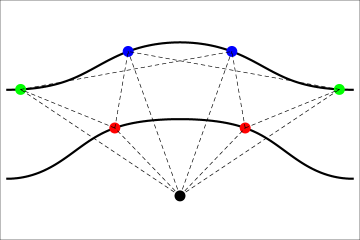
Figure 8. A representation of seven points in $\mathbb{CP}^{2}$ all a distance $2\pi/3$ from $[\mathbf{z}_{1}],[\mathbf{z}_{2}].$ Pairs joined by dashed edges are also $2\pi/3$ apart.

References

- [1] Anandan, J., and Aharonov, Y. Geometry of quantum evolution. Phys. Rev. Lett. 65 (1990), 1697.
- [2] Appleby, D. M. Symmetric informationally complete-positive operator valued measures and the extended Clifford group. J. Math. Phys. 46, 5 (2005), 052107.
- [3] Appleby, D. M., Fuchs, C. M., and Zhu, H. Group theoretic, Lie algebraic and Jordan algebraic formulations of the SIC existence problem. Quantum Inf. Comp. 15 (2015), 61–94.
- [4] Appleby, D. M., Yadsan-Appleby, H., and Zauner, G. Galois automorphisms of a symmetric measurement. Quantum Inf. Comp. 13 (2014), 672–720.
- [5] Armstrong, J., Povero, M., and Salamon, S. Twistor lines on cubic surfaces. Rend. Sem. Mat. Univ. Pol. Torino 71, 3–4 (2013), 317–338.
- [6] Arnold, V. I. Mathematical Methods of Classical Mechanics, second edition. Springer, Berlin, 1989.
- [7] Ashtekar, A., and Schilling, T. A. Geometrical formulation of quantum mechanics. In On Einstein’s Path: Essays in Honor of Engelbert Schucking, A. Harvey, Ed. Springer, Berlin, 1998.
- [8] Bengtsson, I., and Zyczkowski, K. Geometry of Quantum States: An Introduction to Quantum Entanglement. Cambridge University Press, 2008.
- [9] Brody, D. C., and Hughston, L. P. Geometric quantum mechanics. J. Geom. Phys. 38 (2001), 19–53.
- [10] Cox, D., Little, J., and O’Shea, D. Ideals, Varieties, and Algorithms. Springer, Berlin, 1992.
- [11] Dang, H. B., Blanchfield, K., Bengtsson, I., and Appleby, D. M. Linear dependencies in Weyl-Heisenberg orbits. Quantum Inf. Processing 12 (2013), 3449–3475.
- [12] Davies, E. B. Quantum Theory of Open Systems. Academic Press, London, 1976.
- [13] Durt, T. About mutually unbiased bases in even and odd prime power dimensions. J. Phys. A: Math. Gen. 38 (2005), 5267.
- [14] Flammia, S. T. On SIC-POVMs in prime dimensions. J. Phys. A: Math. Gen. 39 (2006), 13483–13493.
- [15] Freed, D. S. On Wigner’s theorem. arXiv:1112.2133.
- [16] Gibbons, G. W. Typical states and density matrices. J. Geom. Phys. 8 (1992), 147–162.
- [17] Gour, G. Construction of all general symmetric informationally complete measurements. J. Phys. A: Math. Theor. 47 (2014), 335302.
- [18] Grassl, M. Computing equiangular lines in complex space. In Mathematical Methods in Computer Science, vol. 5393 of Lecture Notes in Computer Science. Springer, 2008, pp. 89–104.
- [19] Greaves, G., Koolen, J. H., Munemasa, A., and Szöllősi, F. Equiangular lines in Euclidean spaces. arXiv:1403.2155.
- [20] Guillemin, V., and Sternberg, S. Symplectic Techniques in Physics. Cambridge University Press, 1990.
- [21] Hoggar, S. G. 64 lines from a quaternionic polytope. Geom. Ded. 69 (1998), 287–289.
- [22] Holevo, A. S. Probabilistic and Statistical Aspects of Quantum Theory. North-Holland, Amsterdam, 1982.
- [23] Horrocks, G., and Mumford, D. A rank 2 vector bundle on with 15000 symmetries. Topology 12 (1973), 63–81.
- [24] Hughston, L. P. d3 SIC-POVMs and elliptic curves. Perimeter Institute seminar (2007), available at http://pirsa.org/07100040/.
- [25] Hughston, L. P. Geometric aspects of quantum mechanics. In Twistor Theory, S. Huggett, Ed. Marcel Dekker, New York, 1995.
- [26] Hughston, L. P. Geometry of stochastic state vector reduction. Proc. Roy. Soc. London A 452 (1996), 953–979.
- [27] Kibble, T. W. B. Geometrization of quantum mechanics. Commun. Math. Phys. 65 (1979), 189–201.
- [28] Kobayashi, S., and Nomizu, K. Foundations of Differential Geometry, Vols I and II. Wiley Classics Library, 1996.
- [29] Lemmens, P. W. H., and Seidel, J. J. Equiangular lines. J. Algebra 24 (1973), 494–512.
- [30] Lora Lamia, N. Kähler, complex, Hermitian geometry: Fubini distance in with computations in dimension . MSc thesis, University of Turin, 2014.
- [31] Mihaylov, G. Toric moment mappings and Riemannian structures. Geom. Dedicata 162 (2013), 129–152.
- [32] Renes, J. M., Blume-Kohout, R., Scott, A. J., and Caves, C. M. Symmetric informationally complete quantum measurements. J. Math. Phys. 45, 6 (2004), 2171–2180.
- [33] Scott, A. J., and Grassl, M. SIC-POVMs: A new computer study. J. Math. Phys. 51, 4 (2010), 042203.
- [34] Steidel, S. Gröbner bases of symmetric ideals. J. Symbolic Comput. 54 (2013), 72–86.
- [35] Sturmfels, B. What is a Gröbner basis? Notices Amer. Math. Soc. 52, 10 (2005), 2–3.
- [36] Szöllősi, F. All complex equiangular tight frames in dimension 3. arXiv:1402.6429.
- [37] Thurston, W. P. Three-Dimensional Geometry and Topology. Vol. 1. Princeton Mathematical Series 35. Princeton University Press, 1997.
- [38] Wang, H.-C. Two-point homogeneous spaces. Annals of Math. 55 (1952), 177–191.
- [39] Welch, L. R. Lower bounds on the maximum cross-correlation of signals. IEEE Trans. Inform. Theory 20 (1974), 397–399.
- [40] Weyl, H. The Theory of Groups and Quantum Mechanics. Dover, 1950.
- [41] Wigner, E. P. Gruppentheorie und ihre Anwendung auf die Quanten mechanik der Atomspektren. Friedrich Vieweg und Sohn, 1931.
- [42] Wooters, W. K. Quantum measurements and finite geometry. Found. Phys. 36, 1 (2006), 112–126.
- [43] Zauner, G. Quantum designs: foundations of a non-commutative design theory. Int. J. Quantum Inf. 9 (2011), 445–507. (Quantendesigns – Grundzüge einer nichtkommutativen Designtheorie, PhD thesis, University of Vienna, 1999).
- [44] Zhu, H. SIC POVMs and Clifford groups in prime dimensions. J. Phys. A: Math. Theor. 43 (2010), 305305.
Lane Hughston
Department of Mathematics, Brunel University London, Uxbridge UB8 3PH, UK
Department of Mathematics, University College London, London WC1E 6BT, UK
St Petersburg State University of Information Technologies, Mechanics and Optics,
Kronwerkskii ave 49, 199034 St Petersburg, Russia
E-mail: lane.hughston@brunel.ac.uk
Simon Salamon
Department of Mathematics, King’s College London, Strand, London WC2R 2LS, UK
E-mail: simon.salamon@kcl.ac.uk