Banana Split: Testing the Dark Energy Consistency with Geometry and Growth

Abstract

We perform parametric tests of the consistency of the standard $w$CDM model in the framework of general relativity by carefully separating information between the geometry and growth of structure. We replace each late-universe parameter that describes the behavior of dark energy with two parameters: one describing geometrical information in cosmological probes, and the other controlling the growth of structure. We use data from all principal cosmological probes: of these, Type Ia supernovae, baryon acoustic oscillations, and the peak locations in the cosmic microwave background angular power spectrum constrain the geometry, while the redshift space distortions, weak gravitational lensing and the abundance of galaxy clusters constrain both geometry and growth. Both geometry and growth separately favor the $\Lambda$CDM cosmology with the matter density relative to critical $\Omega_{M}\simeq 0.3$. When the equation of state is allowed to vary separately for probes of growth and geometry, we find again a good agreement with the $\Lambda$CDM value ($w\simeq-1$), with the major exception of redshift-space distortions which favor less growth than in $\Lambda$CDM at 3-$\sigma$ confidence, favoring the equation of state $w^{\rm grow}\simeq-0.8$. The anomalous growth favored by redshift space distortions has been noted earlier, and is common to all redshift space distortion data sets, but may well be caused by systematics, or be explained by the sum of the neutrino masses higher than that expected from the simplest mass hierarchies, $m_{\nu}\simeq 0.45$ eV. On the whole, the constraints are tight even in the new, larger parameter space due to impressive complementarity of different cosmological probes.

I Introduction

The discovery of the acceleration of the universe’s expansion Riess et al. (1998); Perlmutter et al. (1999) has brought about one of the most interesting and important questions in modern physics: what is the nature of dark energy responsible for the acceleration? Arguably the simplest and certainly the most popular candidate is vacuum energy, responsible for the cosmological constant term in Einstein’s equations. The cosmological constant-dominated universe ($\Lambda$CDM), where the energy density today is dominated by $\sim 75\%$ dark energy and $\sim 25\%$ matter, is well fit by essentially all current data. Nevertheless, many alternatives to vacuum energy have been discussed over the past 15 years or so. Some of these alternatives involve scalar fields or other light degrees of freedom which obey the standard equations of general relativity but lead to a richer dynamics and a different expansion rate and growth of structure than $\Lambda$CDM and, therefore, can in principle be distinguished from the latter. Nevertheless, in all such explanations the growth of linear structures (matter density contrast $\delta\equiv\delta\rho_{M}/\rho_{M}\ll 1$) evolves independently of the spatial scale $k$ and can be obtained, well within the Hubble radius, by solving the equation

$$\ddot{\delta}+2H\dot{\delta}-4\pi G\rho_{M}\delta=0,$$ (1)

where $H$ is the Hubble parameter and dots are derivatives with respect to time. For a review of dark energy observations and theory, see e.g. Frieman et al. (2008).

A very different class of explanations fall in the category of modified gravity (for an excellent review, see Joyce et al. (2015)). Here the acceleration of the universe is caused by the corrections to general relativity at large scales. These corrections obviously have to be suppressed at Solar-System-size and perhaps galactic-size scales, and there are several known mechanisms that do just that. Because the gravity theory is truly modified, the growth is generally not given by Eq. (1), and moreover the growth is not necessarily scale independent any more. Therefore, for a fixed expansion rate $H(t)$ — or, for that matter, the comoving distance as a function of redshift $r(z)$ or any other geometric quantity — the growth of linear structures is different in standard and modified gravity. Moreover, the time dependence of $\delta$ is in general $k$-dependent in modified gravity.

Comparing the geometrical quantities to the growth of structure is, therefore, an excellent way to test the consistency of the fiducial standard-gravity cosmological model; this was pointed out soon after the discovery of the accelerating universe Ishak et al. (2006); Zhan et al. (2009); Mortonson et al. (2009, 2010); Acquaviva and Gawiser (2010); Vanderveld et al. (2012). The idea is to separately measure the redshift evolution of the geometrical quantities such as distances on the one hand, and growth of structure on the other, and test whether or not they are related by Eq. (1). This approach is the same in spirit to a much more extensive body of work on parameterizing the nonrelativistic and relativistic gravitational potentials, $\Phi$ and $\Psi$ (which govern the motion of matter and of light, respectively), and testing in whether they are the same or not Zhao et al. (2010); Bean and Tangmatitham (2010); Zhao et al. (2012); Hojjati et al. (2012); Dossett et al. (2011a, b); Silvestri et al. (2013). In practice and implementation, however, the two approaches are very complementary.

Our goal is to make a major step forward in developing the first one of the aforementioned consistency tests — testing the consistency of $w$CDM (the generalization of $\Lambda$CDM where the dark energy equation of state $w$ is allowed to take constant values other than the $\Lambda$CDM value of -1) by separately constraining the geometry and growth in major cosmological probes of dark energy. This program has been started very successfully by Wang et al. (2007) (see also (Zhang et al., 2005; Chu and Knox, 2005; Abate and Lahav, 2008) which contained very similar ideas), who used data available at the time; the constraints however were weak. Our overall philosophy and approach are similar as those in Refs. Wang et al. (2007); Zhang et al. (2005); Chu and Knox (2005); Abate and Lahav (2008), but we benefit enormously from the new data and increased sophistication in understanding and modeling them, as well as the availability of a few additional cosmological probes not available in 2007.

The paper is divided as follows: we present the reasoning behind our approach in Sec. II. In Sec. III we review the cosmological probes used in the analysis. A review of the analysis method is provided in Sec. IV, and we present our constraints on parameters in Sec. V. We discuss these results in Sec. VI, and give final remarks in Sec. VII.

II Philosophy of our Approach

We would like to perform stringent but general consistency tests of the currently favored $\Lambda$CDM cosmological model with $\sim$25% dark plus baryonic matter and $\sim$75% dark energy, as well as the more general $w$CDM model. The $\Lambda$CDM model, favored since even before the direct discovery of the accelerating universe (e.g. Krauss and Turner (1995)), is in excellent agreement with essentially all cosmological data, despite occasional mild warnings to the contrary (Scolnic et al. (2014); Cheng and Huang (2014); Xia et al. (2013); Shafer and Huterer (2014)). There has been a huge amount of effort devoted to tests alternative to $w$CDM – most notably, modified gravity models where modifications to Einstein’s General Theory of Relativity, imposed to become important at late times in the evolution of the universe and at large spatial scales, make it appear as if the universe is accelerating if interpreted assuming standard general relativity.

Here we take a complementary approach, and study the internal consistency of the $w$CDM model itself, without assuming any alternative model. We split the cosmological information describing the late universe into two classes:

• Geometry: expansion rate $H(z)$ and the comoving distance $r(z)$, and associated derived quantities.

• Growth: growth rate of density fluctuations in linear ($D(z)\equiv\delta(z)/\delta(0)$) and nonlinear regime.

Regardless of the parametric description of the geometry and growth sectors, one thing is clear: in the standard model that assumes general relativity with its usual relations between the growth and distances, the split parameters $X_{i}^{\rm geom}$ and $X_{i}^{\rm grow}$ have to agree – that is, be consistent with each other at some statistically appropriate confidence level. Any disagreement between the parameters in the two sectors, barring unforeseen remaining systematic errors, can be interpreted as the violation of the standard cosmological model assumption.

The split parameter constraints provide very general, yet powerful, tests of the dominant paradigm. They can be compared to more specific parameterizations of departures from general relativity — for example, the $\gamma$ parametrization Linder (2005), or the various schemes of the aforementioned comparison of the Newtonian potentials. Our approach is complementary to these more specific parameterizations: while perhaps not as powerful in specific instances, it is equipped with more freedom to capture departures from the standard model.

Cosmological Probe	Geometry	Growth
SN Ia	$H_{0}D_{L}(z)$	—–
BAO	$\displaystyle\left(\frac{D_{A}^{2}(z)}{H(z)}\right)^{1/3}/r_{s}(z_{d})$	—–
CMB peak loc.	$R\propto\sqrt{\Omega_{m}H_{0}^{2}}\,D_{A}(z_{*})$	—–
Cluster counts	$\displaystyle\frac{dV}{dz}$	$\displaystyle\frac{dn}{dM}$
Weak lens 2pt	$\displaystyle\frac{r^{2}(z)}{H(z)}W_{i}(z)W_{j}(z)$	$P\left(k=\displaystyle\frac{\ell}{r(z)}\right)$
RSD	$F(z)\propto D_{A}(z)H(z)$	$f(z)\sigma_{8}(z)$

Table 1: Summary of cosmological probes that we used and aspects of geometry and growth that they are sensitive to. The assignments in the second and third column are necessarily approximate given the short space in the table; more detail is given in respective sections covering our use of these cosmological probes. Here $r_{s}(z_{d})$ refers to the sound horizon evaluated at the baryon drag epoch $z_{d}$.

Most of the cosmological measurements involve large amounts of raw data, and their information is often compressed into a very small number of meta-parameters. For example, weak lensing shows the two-point correlation function, cluster number counts are given in mass bins, while baryon acoustic oscillations, cosmic microwave background, and redshift space distortion information is often captured in a small number of meta-parameters which are defined and presented below. [Type Ia supernovae are somewhat of an exception, since we use individual magnitude measurements from each SN from the beginning.] Given that in some cases one assumes the cosmological model (often $\Lambda$CDM) to derive these intermediate parameters, the question is whether we should worry about using the meta-parameters to constrain the wider class of cosmological models where growth history is decoupled from geometry. Fortunately, in this particular case our constraints are robust: certainly for surveys that specialize in either geometry and growth alone, the meta-parameters are de facto correct by construction, and capture nearly all cosmological information of interest. For probes that are sensitive to both growth and geometry, e.g. weak lensing and cluster counts, the quantities used for the analysis — correlation functions and number counts, respectively — provide a general enough representation of the raw data that one can relax the assumption that growth and geometry are consistent without the loss of robustness and accuracy.

III Observational Probes

We now discuss, in turn, the various cosmological probes used in this work: Type Ia supernovae, the cosmic microwave background fluctuation power spectrum, baryon acoustic oscillations, cluster counts, weak gravitational lensing, and redshift space distortions.

In Table 1 we summarize quantities or aspects of each cosmological probe that are sensitive to geometry, and those that depend on growth. In the following subsections, we describe in more detail the cosmological probes, the quantities that they measure, and the data sets that we use.

III.1 Type Ia Supernovae

Type Ia supernovae (SNIa) are the principal probes of geometry of the universe, as they directly measure the luminosity distance. Thus SNIa are specialized in probing the geometrical parameters.

Each SNIa provides an independent measurement of the magnitude-redshift relation. The theoretically expected apparent magnitude of the supernova at redshift $z$ is

$$m_{\text{th}}(z)=5\log_{10}(H_{0}D_{L}(z))+\mathcal{M},$$ (2)

where $\mathcal{M}$ is a nuisance parameter combining the intrinsic magnitude of the supernova with the Hubble parameter $H_{0}$ (Perlmutter et al., 1999). Therefore, each SNIa constrains the luminosity distance $D_{L}(z)$, with one overall nuisance parameter $\mathcal{M}$ to be determined from the data as well.

There are several properties of supernovae that can change the magnitude of a supernova; these must be corrected for. The stretch (or broadness) of a supernova light curve is correlated with its brightness. Similarly, the color of a supernova is also correlated with its brightness — the broader and bluer the supernova light curve, the brighter that supernova will be. We correct for these effects by writing the magnitude as Conley et al. (2011); Ruiz et al. (2012)

$$m=m_{\text{th}}-\alpha_{s}\ (s-1)+\beta_{\mathcal{C}}\ \mathcal{C},$$ (3)

where $s$ is the stretch and $\mathcal{C}$ the color of each SNIa, and $\alpha_{s}$ and $\beta_{\mathcal{C}}$ are additional, global nuisance parameters.

In addition to the statistical errors for each supernova measurement, we also include the correlated systematic errors between each supernova measurement Conley et al. (2011); Ruiz et al. (2012). The covariance matrix resulting from these correlations is also a function of $\alpha_{s}$ and $\beta_{\mathcal{C}}$. Finally, we take into account host-galaxy effects in the value of $\mathcal{M}$ Conley et al. (2011); Shafer and Huterer (2014) in our analysis. We allow two values of $\mathcal{M}$, one for supernovae in lower-mass host galaxies and one for higher-mass galaxies. These two $\mathcal{M}$’s are then marginalized over analytically. See Appendix C of Conley et al. (2011) for details.

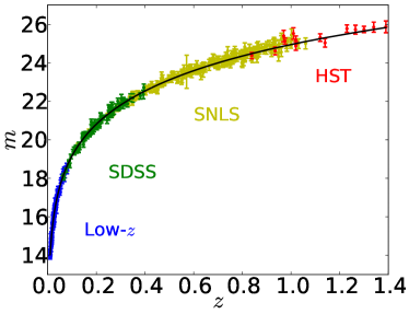
Figure 1: Plot showing the set of 472 supernovae used in this work. Error bars are from diagonal-only statistical errors. The black line shows the best-fit $\Lambda$CDM model with parameter values from column 2 of Table 7.

We use the Supernova Legacy Survey (SNLS) data compilation from Conley et al. (2011), which contains 472 supernovae from various surveys, including SNLS itself, the Sloan Digital Sky Survey (SDSS), some high redshift supernovae observed by the Hubble Space Telescope (HST), and a selection of low-$z$ supernovae observed by various ground-based telescopes, collectively named the “Low-$z$” sample. Supernova observations are summarized in Table 2.

Source	$N_{\mathrm{SN}}$	Redshift range
Low-$z$	123	$0.01-0.1$
SDSS	93	$0.06-0.4$
SNLS	242	$0.08-1.05$
HST	14	$0.7-1.4$

Table 2: Summary of SNIa observations included in this analysis, showing the number of SN included from each survey and the approximate redshift ranges.

III.2 CMB Peak Location

The hot and cold spots of the cosmic microwave background (CMB) anisotropies provide an excellent standard ruler: their angular separation, combined with the sound horizon distance that is independently well determined (from the CMB peaks’ morphology), provides a single yet accurate measurement of the angular diameter distance $D_{A}(z_{*})$ to recombination. In addition to being very high-redshift, this measurement of $D_{A}(z_{*})$ is unique in that the physical matter density $\Omega_{M}h^{2}$ is essentially fixed by the CMB peaks’ height. This is why the CMB peak location measurement traces out a very complementary degeneracy direction in the $\Omega_{M}$–$w$ plane to low-redshift measurements of distance Frieman et al. (2003).

For simplicity and clarity, we only use the geometrical measurement provided by the CMB acoustic peaks’ locations. The integrated Sachs-Wolfe (ISW) effect of dark energy imprints on the CMB angular power spectrum on very large scales adds very little to the information due to large cosmic variance. CMB is also sensitive to the physics at the last-scattering surface Zahn and Zaldarriaga (2003), but recall that we decided to study the growth vs. geometry only in the late universe, when dark energy becomes significant. Our use of the peaks’ location only obviates the use the numerical CMB codes that evaluate a full set of Einstein-Boltzmann equations, and speeds on this aspect of computation by a factor of $O(100)$.

Therefore, we use the aforementioned angular diameter distance to last scattering with $\Omega_{M}h^{2}$ fixed, which is sometimes referred to as the “shift parameter” $R$, defined as

$$R=\sqrt{\Omega_{m}H_{0}^{2}}\,(1+z_{*})D_{A}(z_{*}).$$ (4)

To obtain a value of $R$, we use the Planck collaboration’s Planck + WP measurements of $r_{*}$ and $\theta_{*}$ Ade et al. (2014); since $\theta_{*}=r_{*}/D_{A}(z_{*})$, we marginalize over these measurements assuming the $\Lambda$CDM cosmological model, as in (Ade et al., 2014) to get a value for $D_{A}(z_{*})$. Combining this with the Planck values of $\Omega_{M}h^{2}$ and $z_{*}$, we obtain

$$R=1.7502\pm 0.0073$$ (5)

for their value of $z_{*}=1090.48$. Being only sensitive to $\Omega_{M}$ and $w$, $R$ presents a handy yet powerful constraint on the late universe. When using the CMB peak information alone, measurement of parameter $R$ in Eq. (5) therefore provides complete information – modulo the aforementioned small ISW contribution – about CMB’s constraint on the late universe.

Once we combine the CMB peaks information with that of other cosmological probes and add the CMB early-universe prior (discussed further below in Sec. IV.1), simply including the $R$ measurement would be inconsistent as $R$ is necessarily correlated with the early universe parameters, e.g. $\Omega_{M}h^{2}$. To do it correctly, we first extract the $5\times 5$ covariance matrix from Planck which contains the $4\times 4$ early universe prior shown in Table 6, plus an additional row and column corresponding to $R$. We than use the $5\times 5$ matrix as our early universe prior that automatically and consistently includes the CMB peaks information. Other probes are then added straightforwardly; see Sec. IV.2 for details.

III.3 Baryon Acoustic Oscillations

Baryonic acoustic oscillations (BAO) are features that arise from the propagating sound waves in the early universe. The distance the sound wave can travel between the Big Bang and decoupling – the sound horizon – imprints a characteristic scale not only in the CMB fluctuations, but also in the clustering two-point correlation function of galaxies. Roughly speaking, the two-point correlation function is enhanced by $\sim 10\%$ at distances of $\sim 100\,h^{-1}{\rm Mpc}$. This latter distance is, similarly to the CMB case, well measured by the early-universe parameters ($\Omega_{M}h^{2}$ and $\Omega_{B}h^{2}$ principally), but where we observe it is dependent on the expansion history of the universe between the time that light from the galaxies is emitted and today.

Specifically, for two galaxies at the same redshift separated by comoving distance $r$ and seen with separation angle $\theta$, we have $\theta=r/D_{A}(z)$ which enables measurement of the angular diameter distance given known separation between galaxies. Similarly, two galaxies at the same angular location but separated by redshift difference $\Delta z$ are separated by comoving distance $r$, with the two quantities related via $\Delta z=rH(z)$. The information from these transverse and radial sensitivities can be conveniently combined into a single quantity, a generalized distance $D_{V}(z_{\text{eff}})$ defined as Eisenstein et al. (2005)

$$D_{V}(z)\equiv\left(\frac{(1+z)^{2}D_{A}^{2}(z)cz}{H(z)}\right)^{1/3}.$$ (6)

The BAO surveys measure $r_{s}(z_{d})/D_{V}(z_{\text{eff}})$ (or its inverse), where $r_{s}(z_{d})$ is the comoving sound horizon at the redshift of the baryon drag epoch $z_{d}$,

$$r_{s}(z)=\frac{1}{\sqrt{3}}\int_{0}^{1/(1+z)}\frac{da^{\prime}}{a^{\prime 2}H(a^{\prime})\sqrt{1+3\rho_{b}/4\rho_{\gamma}}}.$$ (7)

In addition to the late-universe parameters, these BAO observable quantities are only sensitive to the early-universe physics via a fixed single combination, the sound horizon $r_{s}(z_{d})$.

Survey	$z_{\text{eff}}$	Parameter	Measurement
6dFGS Beutler et al. (2011)	0.106	$r_{s}/D_{V}$	$0.336\pm 0.015$
SDSS LRG Padmanabhan et al. (2012)	0.35	$D_{V}/r_{s}$	$8.88\pm 0.17$
BOSS CMASS Anderson et al. (2012)	0.57	$D_{V}/r_{s}$	$13.67\pm 0.22$

Table 3: BAO data measurements used here, together with the effective redshift for the corresponding galaxy sample.

It is important to note that the radiation term must be included in $H(a)$ in Eq. (7). The radiation energy density relative to critical is $\Omega_{r}=\Omega_{M}a_{\text{eq}}$, where $a_{\text{eq}}=1/(1+z_{\text{eq}})$ is the scale factor at matter-radiation equality and

$$z_{\text{eq}}\approx 25000\ \Omega_{M}h^{2}\left(\frac{T_{\text{CMB}}}{2.7\text{K}}\right)^{-4}.$$ (8)

The ratio of the baryonic density to the radiation density can be approximated as

$$\frac{3\rho_{b}}{4\rho_{\gamma}}\approx 31500\ \Omega_{B}h^{2}\left(\frac{T_{\text{CMB}}}{2.7\text{K}}\right)^{-4}a.$$ (9)

We assume a value of $T_{\text{CMB}}=2.7255\text{K}$.

The redshift of the drag epoch can be approximated by the fitting formula Eisenstein and Hu (1999)

$$z_{d}=\frac{1291(\Omega_{M}h^{2})^{0.251}}{1+0.659(\Omega_{M}h^{2})^{0.828}}\left[1+b_{1}(\Omega_{B}h^{2})^{b_{2}}\right],$$ (10)

where

$$b_{1} =0.313(\Omega_{M}h^{2})^{-0.419}\left[1+0.607(\Omega_{M}h^{2})^{0.674}\right],$$ (11)

$$b_{2} =0.238(\Omega_{M}h^{2})^{0.223}.$$

We use three sources of data for BAO constraints: the Six-degree-Field Galaxy Survey (6dFGS) Beutler et al. (2011), the SDSS Luminous Red Galaxies (SDSS LRG) Padmanabhan et al. (2012), and the SDSS-III DR9 Baryon Oscillation Spectroscopic Survey (BOSS) Anderson et al. (2012). These measurements and the corresponding redshift ranges of their galaxy samples are summarized in Table 3.

III.4 Cluster Counts: MaxBCG

Counts of galaxy clusters are a particularly useful probe for this work, as they probe both growth and geometry (for a review see Allen et al. (2011)). Cluster number density and its dependence on the cosmological model are calibrated from N-body simulations; they are determined by the growth of structure. On the other hand, the volume is purely a geometric quantity that is straightforwardly calculated from first principles. Product of the number density and volume gives the number of clusters in some mass and redshift range, which can be compared to measurements.

More specifically, the number of clusters within some mass and redshift range is

$$N=\int dM\ dz\ \frac{dn}{dM}\frac{dV}{dz}\psi(M)\phi(z)$$ (12)

where $dn/dM$ is the halo mass function, $dV/dz$ is the comoving volume per unit redshift, and $\psi(M)$ and $\phi(z)$ are the top-hat functions that specify our binning in mass and redshift, that is, $\psi(M)=1$ if $M$ is in the mass bin of interest and 0 otherwise, and likewise for $\phi(z)$.

Here we use the measurements from the MaxBCG cluster catalog (Rozo et al. (2010)), based on measurements from the Sloan Digital Sky Survey Koester et al. (2007). A key proxy for measuring cluster masses is “richness”, defined as the number of galaxies in $R_{200}$, the radius at which the average density of the cluster is 200 times that of the critical density of the universe. The richness-mass relation has been calibrated using weak gravitational lensing measurements from Johnston et al. (2007). For clarity and completeness, we give further details of the Rozo et al. (2010) analysis that we adopt in Appendix A.

Cluster mass and redshift are not directly observable, but instead we rely on cluster richness-mass relation and photometric redshift of cluster galaxy members, respectively. We define $P(N_{200}|M)$ to be the probability that a cluster of mass $M$ has a richness $N_{200}$, and $P(z_{\text{photo}}|z)$ to be the probability that a cluster at redshift $z$ is observed with a photometric redshift $z_{\text{photo}}$. We redefine $\psi=\psi(N_{200})$ and $\phi=\phi(z_{\text{photo}})$. The expected number of clusters then becomes

$$\langle N\rangle=\int dM\,dz\,\frac{dn}{dM}\frac{dV}{dz}\langle\psi|M\rangle\langle\phi|z\rangle$$ (13)

where we introduce the probability weighting functions

$$\langle\psi|M\rangle =\int dN_{200}\,P(N_{200}|M)\psi(N_{200}),$$ (14)

$$\langle\phi|z\rangle =\int dz_{\text{photo}}\,P(z_{\text{photo}}|z)\phi(z_{\text{photo}}).$$ (15)

Here $P(z_{\text{photo}}|z)$ is modeled as a Gaussian distribution as discussed in Rozo et al. (2010). Meanwhile, $P(N_{200}|M)$ is modeled as log-normal distribution, with the mean $\langle\ln N_{200}|M\rangle$ assumed to vary linearly with mass, resulting in two free parameters and an unknown variance which is also treated as free parameter. These parameters are marginalized in the analysis; see Appendix A for details.

In a similar fashion, the expected total mass of clusters in a richness bin is given by

$$\langle N\bar{M}\rangle=\beta\int dM\,dz\frac{dn}{dM}\frac{dV}{dz}\langle\psi|M\rangle\langle\phi|z\rangle.$$ (16)

where another nuisance parameter $\beta$ is introduced to take into account the uncertainty in the overall calibration of mass; $\bar{M}_{\text{obs}}\rightarrow\beta\bar{M}_{\text{obs}}$. The comoving volume is simply

$$\frac{dV}{dz}=\Omega_{\text{sky}}\frac{r^{2}(z)}{H(z)}$$ (17)

where $\Omega_{\text{sky}}=2.254\text{ sr}$ is the solid angle covered by SDSS and $r(z)$ is the comoving distance.

Finally, we use the Tinker mass function Tinker et al. (2008) for our halo mass function $dn/dM$. The mass function requires the matter power spectrum as input, and to speed up the code we calculate $P(k)$ semianalytically; for that purpose we use the Eisenstein and Hu transfer function Eisenstein and Hu (1999). We have checked that our calculation leads to negligible differences in the results compared to one using CAMB’s matter power spectrum as input.

III.5 Weak Lensing Shear: CFHTLens

Recent measurements by the Canada-France Hawaii Telescope Lensing Survey (CFHTLenS) provide a very appealing test bed to apply our methodology and test the consistency of the cosmological model, as weak lensing is sensitive to both growth and distance.

The CFHTLenS survey Erben et al. (2013); Heymans et al. (2012) covered 154 square degrees over a period of five years in five wavebands (ugriz). The resolved galaxy density is 17/arcmin². What is particularly appealing for cosmological tests is that the survey is very deep (mean redshift $z_{\rm mean}\simeq 0.75$), implying that potentially strong constraints on the temporal evolution of the effects of dark energy – and, therefore, the growth and geometry parameters – can be achieved. A detailed analysis by the CFHTLenS team made the shape measurements and obtained the photometric redshift of galaxies, all the while dealing with a host of observational and astrophysical systematic errors. The results are publicly available at the survey web site. We use their blu_sample data, which were shown in Heymans et al. (2012) to have a negligible intrinsic alignment signal. The data are given in six tomographic redshift bins, and presented at five different angles, $\theta=\{1.73^{\prime\prime},3.75^{\prime\prime}.8.13^{\prime\prime},17.6^{\prime\prime},37.9^{\prime\prime}\}$. The data is given for the two 2-point correlation functions $\xi^{+}$ and $\xi^{-}$, defined as

$$\xi_{ij}^{\pm}=\frac{1}{2\pi}\int_{0}^{\infty}d\ell\,\ell\,P^{\kappa}_{ij}(\ell)J^{\pm}(\ell\theta),$$ (18)

where $\ell$ is the multipole, and $J^{+}(x)\equiv J_{0}(x)$ and $J^{-}(x)\equiv J_{4}(x)$. Here $P^{\kappa}$ is the weak lensing convergence power spectrum, that is, the two-point correlation function of the convergence field on the sky, given as a function of the multipole $\ell$. In the Limber approximation, which only includes modes perpendicular to the line of sight and is an excellent approximation at scales of interest, the convergence power is given as

$$P^{\kappa}_{ij}(\ell)=\int dz\,\frac{r^{2}(z)}{H(z)}W_{i}(z)W_{j}(z)\,P\left(k=\frac{\ell}{r(z)}\right),$$ (19)

where $r(z)$ and $H(z)$ are the comoving distance and Hubble parameter respectively, and the weight functions involve the distribution of galaxies $dN/dz$ in each redshift bin

$$W_{i}(z)=\frac{3}{2}\Omega_{M}H_{0}^{2}g_{i}(z)(1+z),$$ (20)

where the weight function is given in terms of the radial distance $\chi=\int dz/H(z)$,

$$g_{i}(\chi(z)) = r(\chi)\int_{\chi}^{\infty}d\chi_{s}n_{i}(\chi_{s})\,\frac{r(\chi_{s}-\chi)}{r(\chi_{s})}$$

$$\longrightarrow r(z)\int_{z}^{\infty}\frac{dz_{s}}{H(z_{s})}n_{i}(z_{s})\,\frac{r(z_{s})-r(z)}{r(z_{s})}.$$

Here the second line holds in the special case of a flat universe which we adopt in the paper, and where $n(z_{s})$ is the distribution of source galaxies in each redshift bin, normalized to $n_{i}(z_{s})dz_{s}=1$, and provided by CFHTLenS for each tomographic bin (see Fig. 1 of Heymans et al. (2012)).

Finally, special attention is required to modeling the power spectrum $P(k)$, given that scales probed are small — consider, for example, that the smallest angle $\theta=1.73^{\prime\prime}$, at the mean redshift of the survey $z\simeq 1$ spans $k\simeq 1h\,{\rm Mpc}^{-1}$, which is in a regime of strongly nonlinear clustering. It is imperative to have an accurate theoretical prediction for the dark matter clustering at these scales which are a “sweet spot” for sensitivity for weak lensing surveys Huterer and Takada (2005). Here we adopt an updated version of the halofit Smith et al. (2003) prescription for nonlinear clustering given by Takahashi et al. (2012). This fit has the same functional form as the original halofit, but with updated parameter values. The formula has been optimized for the dark energy equation of state $w\simeq-1$, justifying its use in this analysis. We find that the Takahashi et al. prescription makes a non-negligible difference relative to the original; for example, the best-fit $\sigma_{8}$ value, in a simplified analysis we ran as a check, moves downwards by $\sim$0.03 relative to the original halofit, returning $\sigma_{8}\simeq 0.74$ (for a fixed $\Omega_{M}=0.3$), in agreement with Heymans et al. (2012).

We also checked the robustness of the data assumptions by verifying that the blue and full data sets from CFHTLens give very similar constraints.

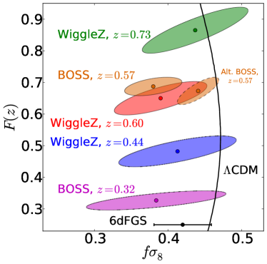
Figure 2: RSD data used in our analysis, shown in the $f\sigma_{8}$–$F$ plane; more details can be found in Table 4. The black line shows the best-fit $\Lambda$CDM model with our best-fit parameter values given in the second column of Table 7. The low-redshift 6dFGS measurement does not have an associated value for $F(z)$, and we therefore only show its horizontal error bar. The BOSS constraint on $F$ is obtained from the covariance of $H(z)$ and $D_{A}(z)$; see Appendix B for details. The dashed error ellipse corresponds to an alternative RSD measurement at $z=0.57$ from Samushia et al. (2014); for details, see Sec. VI.

III.6 Redshift Space Distortions

Redshift space distortions (RSD) refer to the effect of how density modes affect velocity distribution of galaxies in their vicinity. Galaxies’ peculiar velocities are imprinted in galaxy redshift surveys in which recessional velocity is used as the line-of-sight coordinate for galaxy positions, leading to an apparent compression of radial clustering relative to transverse clustering on large spatial scales (a few tens of Mpc). On smaller scales (a few Mpc), one additionally observes the “finger-of-God” elongation Jackson (1972) due to nonlinear effects. The spatial clustering of galaxies is affected on scales corresponding to the size of the largest objects (galaxy clusters) and larger, all the way up to $\sim 100$Mpc. Measuring the clustering at these scales and at various redshifts provides valuable information about the growth of structure across cosmic history.

RSD measurements are uniquely sensitive to the combination of cosmological parameters $f(a)\sigma_{8}(a)$ (often just referred to as $f\sigma_{8}$) Song and Percival (2009), where $f(a)\equiv d\ln D/d\ln a$ and $D(a)$ is the linear growth factor.

In addition to pure growth information, however, we must take into account the geometrical aspect of the RSD measurements, which comes about from the breaking of underlying isotropy of galaxy clustering when observed in redshift space. The effect is accurately captured by the parameter which serves to compare clustering in the radial and tangential directions Ballinger et al. (1996); Matsubara and Suto (1996); Simpson and Peacock (2010), and which has been motivated by the original analysis by Alcock and Paczynski (1979)

$$F(z)\equiv(1+z)H(z)D_{A}(z)/c$$ (22)

where $H(z)$ is the Hubble parameter and $D_{A}(z)$ is the angular distance. Intuitively, the comoving diameter a spherical object (or, more generally, a feature in the clustering of galaxies) $ds$ at redshift $z$ is related to its angular size on the sky $\Delta\theta$ by $ds=D_{A}(z)\Delta\theta$. The diameter of the feature can also be related to its redshift extent $\Delta z$ via $ds=c\Delta z/[(1+z)H(z)]$. By comparing the angular and redshift dimensions of the feature (i.e. measuring $\Delta\theta/\Delta z$) one can then determine the parameter combination given in Eq. (22). Alternatively, the effect is captured by the separate but correlated measurements of $H(z)$ and $D_{A}(z)$. These parameters all measure geometric effects and thus grant RSD the ability to test both geometry and growth.

We use a compilation of measurements of $f\sigma_{8}$, $F(z)$, $H(z)$, and $D_{A}(z)$ from a number of spectroscopic surveys; these are summarized in Table 4 and illustrated in Fig. 2.

$z$	Parameter	Measurement (diag)	Survey
$0.067$	$f\sigma_{8}$	$0.42\pm 0.06$	6dFGS Beutler et al. (2012)
$0.32$	$H(z)$	$78.1\pm 7.1$	BOSS Low-z Chuang et al. (2013)
$0.32$	$D_{A}(z)$	$950\pm 61$	BOSS Low-z Chuang et al. (2013)
$0.32$	$f\sigma_{8}$	$0.38\pm 0.10$	BOSS Low-z Chuang et al. (2013)
$0.44$	$F(z)$	$0.48\pm 0.05$	WiggleZ Blake et al. (2012)
$0.44$	$f\sigma_{8}$	$0.41\pm 0.08$	WiggleZ Blake et al. (2012)
$0.57$	$H(z)$	$97.1\pm 5.5$	BOSS CMASS Chuang et al. (2013)
$0.57$	$D_{A}(z)$	$1351\pm 60$	BOSS CMASS Chuang et al. (2013)
$0.57$	$f\sigma_{8}$	$0.38\pm 0.04$	BOSS CMASS Chuang et al. (2013)
$0.60$	$F(z)$	$0.65\pm 0.05$	WiggleZ Blake et al. (2012)
$0.60$	$f\sigma_{8}$	$0.39\pm 0.06$	WiggleZ Blake et al. (2012)
$0.73$	$F(z)$	$0.87\pm 0.07$	WiggleZ Blake et al. (2012)
$0.73$	$f\sigma_{8}$	$0.44\pm 0.07$	WiggleZ Blake et al. (2012)

Table 4: RSD measurements from various surveys. Each line shows the effective redshift associated with the data point, the measured parameter, the value of that parameter with associated diagonal error, and the data point’s associated survey. Measurements from the same survey are correlated; (Beutler et al., 2012; Chuang et al., 2013; Blake et al., 2012); for brevity we show the diagonal errors (i.e. square roots of parameter variances) here and the full covariance matrices in Appendix B.

IV Parameters and analysis

IV.1 Parameter space

We adopt the following set of fundamental cosmological parameters

$$\vec{\textbf{p}}^{\text{fund}}=\{\Omega_{M},\Omega_{M}h^{2},\Omega_{B}h^{2},w,10^{9}A,n_{s}\}$$ (23)

where $\Omega_{M}$ and $\Omega_{B}$ are the energy densities in matter and baryons relative to critical density, $w$ is the equation of state of dark energy, $A$ is the amplitude of the primordial curvature power spectrum on scale of 0.05 Mpc^-1, and $n_{s}$ is the scalar spectral index of curvature perturbations. We also include the nuisance parameters

$$\vec{\textbf{p}}^{\text{nuis}}=\{\alpha_{s},\beta_{\mathcal{C}},\langle\ln N|M_{1}\rangle,\langle\ln N|M_{2}\rangle,\sigma_{NM},\beta\},$$ (24)

where $\alpha_{s}$ and $\beta_{\mathcal{C}}$ are the supernovae nuisance parameters, while the others enter the cluster count analysis. Our analysis also produces constraints on several derived parameters,

$$\vec{\textbf{p}}^{\text{deriv}}=\{\sigma_{8},h;\sigma_{MN}\}.$$ (25)

Here, $\sigma_{MN}$ is the scatter of the richness for a given mass (opposed to $\sigma_{NM}$, which is the scatter of the mass for a given richness), and is considered a derived nuisance parameter.

Throughout we assume a constant equation of state parameter $w$ for analyses, as well as a flat universe ($\Omega_{K}=0$). The latter assumption effectively assumes standard inflation, and also has a very practical benefit of improving the convergence of the parameter constraints. At any rate, in this paper we are interested in testing the consistency of the dark energy sector, which is typically unrelated to the flatness of the universe. In addition, we set the sum of neutrino masses to $m_{\nu}=0.06$ eV, which is consistent with atmospheric and solar data on neutrino flavor oscillations and a normal hierarchy between individual mass eigenstates Beringer et al. (2012). Note that, in our extended tests in Sec. VI, we also vary the neutrino mass $m_{\nu}$. The number of neutrino species is held fixed at $N_{\nu}=3.046$ throughout the analysis, as predicted by the standard model.

We adopt priors on $\Omega_{M}$, $\sigma_{NM}$, $\beta$, and $\sigma_{MN}$ from Rozo et al. (2010). In addition, we add very weak top-hat priors on $h$, $w$ and $n_{s}$. See Table 5 for details.

We also impose a multidimensional Gaussian prior based on Planck constraints on $\Omega_{M}h^{2}$, $\Omega_{B}h^{2}$, $10^{9}A$, and $n_{s}$; we term this the early-universe prior (“EU” for short in our plots). While we would have ideally liked to run our analyses without this prior, we find that the MCMC runs without the prior have difficulty converging in the large parameter space with split geometry and growth late-universe parameters. The early-universe prior correlation matrix is calculated from Planck $\Lambda$CDM (+ lowl) MCMC chains Ade et al. (2014); see Table 6. The square roots of the diagonal entries of the full covariance matrix prior – the unmarginalized errors of the prior – are shown in Table 5. We apply this full prior covariance to RSD, WL and clusters, and the overall combined constraint. In the case of BAO, we apply only information coming from the $2\times 2$ subset of this matrix containing $\Omega_{M}h^{2}$ and $\Omega_{B}h^{2}$, corresponding to the sound horizon (“SH” in our plots). The Planck prior changes very little if one assumes the underlying Planck $w$CDM model instead of $\Lambda$CDM, as has been verified explicitly by the authors, implying that it should represent the early-universe information with the sufficient accuracy even when the late-universe parameters have been split.

Parameter	Priors	Geometry	Growth
$\Omega_{M}$	[0.05, 0.95]	✓	✓
$\Omega_{M}h^{2}$	$0.1423\pm 0.0029$5		✓
$\Omega_{B}h^{2}$	$0.02207\pm 0.00033$5		✓
$w$	[-2, 0]	✓	✓
$10^{9}A$	$2.215\pm 0.16$5		✓
$n_{s}$	[0.9, 1.1], $0.9616\pm 0.0094$5		✓
$\sigma_{8}$	—	derived par.
$h$	[0.5, 1.0]	derived par.
$\alpha_{s}$	—	nuisance par.
$\beta_{\mathcal{C}}$	—	nuisance par.
$\langle\ln N|M_{1}\rangle$	—	nuisance par.
$\langle\ln N|M_{2}\rangle$	—	nuisance par.
$\sigma_{NM}$	[0.1, 1.5]	nuisance par.
$\beta$	[0.5, 1.5], $1.0\pm 0.06$	nuisance par.
$\sigma_{MN}$	$0.45\pm 0.1$	der. nuis. par.

Table 5: Parameters used in our analysis. The first seven parameters lying above the horizontal line are the fundamental quantities that we varied in the Markov chains. The next two parameters are derived from the fundamental parameters. Those in the final sections are nuisance parameters, again separated into fundamental (six) and derived (one). In the ’Priors’ column, notation $[a,b]$ indicates a flat prior between the end points $a$ and $b$, while $c\pm d$ indicates a Gaussian prior with mean $c$ and standard deviation $d$. For the basic set of cosmological parameters (i.e. the first six above), we include information about whether they enter the geometry or growth in the final two columns. If a parameter is found in both columns, it is necessarily a split parameter.

IV.2 Likelihood

We assume that the likelihood is Gaussian in suitably chosen meta-parameters for each cosmological probe. We assign the individual likelihoods as follows:

• SNIa: the data vector consists of SN magnitudes, and we calculate the full off-diagonal covariance matrix that takes into account errors in magnitude, stretch factor, color, redshift, and gravitational lensing. See Appendix C of Conley et al. (2011) for details.

• CMB peak location: the data vector consists of the single measurement of the “shift parameter” $R$; see Eq. (4). In the combined-probe analysis, we account for the correlation of $R$ and the early-universe parameters, as explained near the end of Sec. III.2.

• BAO: data vector and corresponding (diagonal) errors are quantities given in Table 3. Because the SDSS and BOSS CMASS samples cover different redshift ranges, and the two are in the northern hemisphere while 6dFGS is in the south, it is a good approximation to ignore correlations between these three surveys.

• Clusters: following Rozo et al. (2010), we utilize both the number counts, and number-weighted mass counts in richness; details are explained in Appendix A.

• Weak lensing (WL): data vector are the correlation functions $\xi_{ij}^{\pm}(\theta)$ given for six redshift bins (so $i\leq j\leq 6$) and for measurements at five values of $\theta$. The total length of the vector is therefore $2\times(6\times 7/2)\times 5=210$. The $210\times 210$ covariance matrix, calculated using numerical simulations, is provided by the CFHTLens team Heymans et al. (2012).

• RSD: data vector and corresponding (diagonal) errors are quantities given in Table 4. The correlation matrices for the off-diagonal errors between data points can be found in Tables 10 and 11 in Appendix B.

	$\Omega_{M}h^{2}$	$\Omega_{B}h^{2}$	$10^{9}A$	$n_{s}$
$\Omega_{M}h^{2}$	$1.00$	$-0.62$	$-0.51$	$-0.84$
$\Omega_{B}h^{2}$	—	$1.00$	$0.56$	$0.70$
$10^{9}A$	—	—	$1.00$	$0.65$
$n_{s}$	—	—	—	$1.00$

Table 6: Correlation matrix corresponding to our early-universe prior (labeled as “EU” in our plots). The correlation matrix is calculated from Planck $\Lambda$CDM (+ lowl) MCMC chains Ade et al. (2014). The square roots of the diagonal entries of the full covariance matrix prior – the unmarginalized errors of the prior – are shown in Table 5. We apply this full prior covariance to RSD, WL and clusters, and the overall combined constraint. In the case of BAO, we apply only information coming from the $2\times 2$ subset of this matrix containing $\Omega_{M}h^{2}$ and $\Omega_{B}h^{2}$, corresponding to the sound horizon (“SH” in our plots).

Figure 3: Fiducial constraints from cosmological probes before the geometry-growth parameter split. We show the 68% and 95% confidence constraints in the $\Omega_{M}$–$\sigma_{8}$ plane assuming $w=-1$ held constant (left panel) and in the $\Omega_{M}$-$w$ plane (right panel). In the labels, “EU” refers to our early universe prior, while “SH” refers to the sound horizon prior; see Table 6 for relevant details.

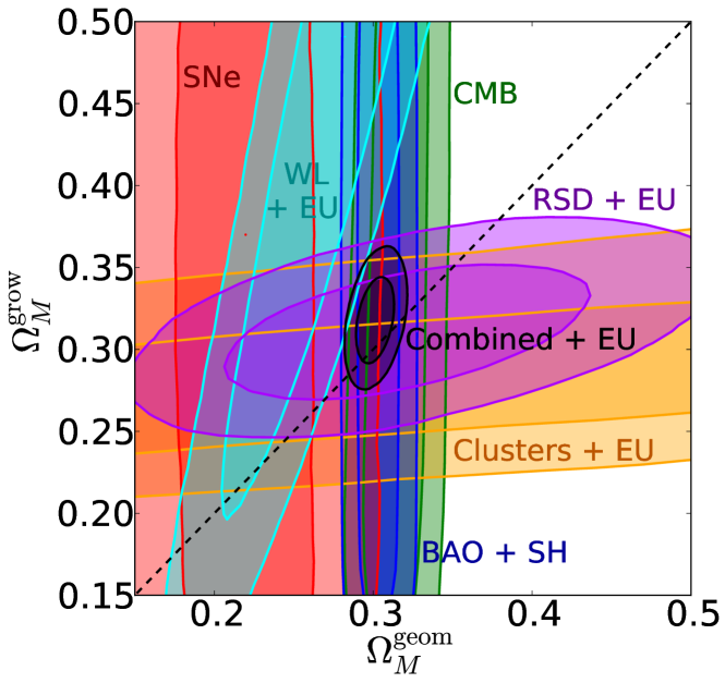
Figure 4: 68% and 95% confidence constraints in the split $\Omega_{M}$ plane with the equation of state held constant at the $\Lambda$CDM value ($w^{\text{geom}}=w^{\text{grow}}=-1$). As in Fig. 3, “EU” refers to our early universe prior, while “SH” refers to the sound horizon prior.

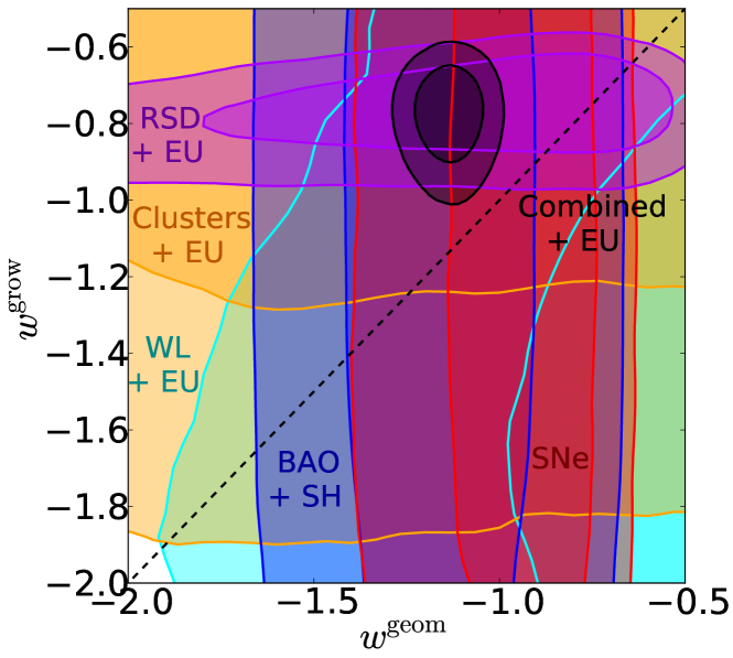
Figure 5: 68% and 95% confidence constraints in the split $w$ plane. Note that the combined $2-\sigma$ contour does not pass through the $w^{\text{geom}}=w^{\text{grow}}$ line. As before, “EU” refers to our early universe prior, while “SH” refers to the sound horizon prior. Individual CMB results have been omitted due to the poor constraints they provide in this plane, but they are included in the combined constraint. See text for details.

The likelihood of the combined cosmological probes is given by the product of individual likelihoods:

$$\mathcal{L}=\mathcal{L}_{\text{SNIa}}\,\mathcal{L}_{\text{CMBpeak}}\,\mathcal{L}_{\text{BAO}}\,\mathcal{L}_{\text{cluster}}\,\mathcal{L}_{\text{WL}}\,\mathcal{L}_{\text{RSD}}\,\mathcal{L}_{\text{prior}}.$$ (26)

The assumption that the individual likelihoods are independent may well be questioned, but it is in practice well justified by the nature of the data sets that we combine. CMB peak location is decoupled from other probes, as it is a much higher-redshift measurement. Similarly, cluster counts are a 1-point correlation function, and as such only weakly coupled to clustering. Weak lensing is expected to be slightly correlated with SNIa, as the latter are also weakly lensed, but the effect is very small for current data.

Perhaps the biggest worry is potential correlation between the BAO and RSD, since these use the same spatial scales (e.g. 32-100 Mpc for the BOSS CMASS sample) and, in the case of both Wigglez and BOSS, the same galaxies. This correlation occurs because the RSD are partially sensitive to the Alcock-Paczynski parameter combination $F(z)\propto H(z)D_{A}(z)$; this in turn may be slightly degenerate with BAO measurements, depending on the treatment of the broadband clustering power in the BAO analysis. Direct estimates indicate that the correlation between the RSD and BAO measured quantities are at the 10% level (e.g. Table 2 of Blake et al. (2012) and Tables 2, 4 and 6 in Chuang et al. (2013)). Therefore, simply multiplying the BAO and RSD likelihoods is justified.

At face value, the Gaussian assumption for the likelihoods might seem risky and unrealistic. Certainly, the exact likelihood in any given probe will not be precisely Gaussian, even if evaluated in parameters that are well measured by the cosmological probes (e.g. the apparent magnitudes of SNIa). Nevertheless, in addition to making the problem vastly more tractable, the assumption of Gaussianity seems to be well justified at this stage: for cosmological models that fit the data well, tails of the distribution are not as important. Had our analysis been oriented toward ruling out $w$CDM – using, for example, Bayesian model-selection techniques – then the analysis would have perhaps warranted a much more careful accounting of the likelihood. This, in turn, would have necessitated a vastly more complex data challenge – for example, fitting theoretical models to the observed galaxy clustering power spectrum, as opposed to the convenient quantity $D_{V}(z)$. In this work, instead, we follow a large body of literature in simplifying our likelihood as Gaussian in the derived parameters since it is expected to be a very good approximation to the truth.

IV.3 Parameter constraints

We use a Markov Chain Monte Carlo (MCMC) algorithm to place constraints on cosmological parameters. The MCMC algorithm estimates the posterior distribution of the cosmological, derived, and nuisance parameters by sampling the parameter space and evaluating the likelihood of each model with the data sets provided. Given the likelihood $\mathcal{L}(\textbf{x}|\textbf{p})$ of the data set x for the parameters p, the posterior distribution is obtained using Bayes’ Theorem

$$\mathcal{P}(\textbf{p}|\textbf{x})=\frac{\mathcal{L}(\textbf{x}|\textbf{p})\mathcal{P}(\textbf{p})}{\int d\textbf{p}\mathcal{L}(\textbf{x}|\textbf{p})\mathcal{P}(\textbf{p})}$$ (27)

where $\mathcal{P}(\textbf{p})$ is the prior probability density. The MCMC algorithm produces the posterior probability in the parameter space including the parameter mean values, covariances, and confidence intervals.

We analyze our models using an MCMC code that one of us (E. R.) developed specifically for this purpose. We initially generate an optimized parameter covariance matrix calculated using several shorter MCMC runs to optimize the MCMC step size and direction and to minimize the overall runtime. The initial 10% of the chains are thrown out, and the resulting chains are analyzed for convergence using the Gelman-Rubin criteria Gelman and Rubin (1992), with a conservative convergence requirement for the convergence parameter of $r<1.03$ across a minimum of six chains for each case. Additionally, the step sizes in parameters are optimized so that they have an acceptance rate of $\sim$35%. The resulting chains are then binned and smoothed with a Gaussian filter for plotting.

V Results

V.1 Unsplit case

Before splitting the late-universe parameters into those sensitive to geometry and growth, we first show the fiducial constraints to make sure they are in reasonably good agreement with similar recent constraints in the literature. The left panel of Fig. 3 shows constraints on the $\Omega_{M}-\sigma_{8}$ plane assuming $w=-1$, while the right panel shows the constraints in the $\Omega_{M}-w$ plane. Note that these plots include marginalization over four other cosmological parameters ($\Omega_{M}h^{2},\Omega_{B}h^{2},10^{9}A$, and $n_{s}$), in addition to several SNIa and cluster nuisance parameters; see Eqs. (23) and (24). We can already see the complementarity of the various cosmological probes: SNIa, BAO and the CMB distance are sensitive only to geometry, so they measure $\Omega_{M}$ and $w$ quite well, but are not sensitive to $\sigma_{8}$. In contrast, WL, RSD and, to a smaller extent, cluster counts constrain (in the case of $w=-1$) the characteristic combinations

$$(\Omega_{M}/0.3)^{0.28}\sigma_{8} =0.799\pm 0.018\quad\mbox{(WL)},$$ (28)

$$(\Omega_{M}/0.3)^{0.04}\sigma_{8} =0.809\pm 0.022\quad\mbox{(RSD)},$$

$$(\Omega_{M}/0.3)^{0.27}\sigma_{8} =0.837\pm 0.021\quad\mbox{(clusters)}.$$

To obtain these best-constrained combinations of $\Omega_{M}$ and $\sigma_{8}$, we simply varied the power $\alpha$ until the error in $(\Omega_{M}/0.3)^{\alpha}\sigma_{8}$ was minimized.

Note that WL constraints favor a somewhat lower value of $\Omega_{M}$ and a higher value of $\sigma_{8}$ than those favored by the combination of other data sets. This has been noted and extensively explored in MacCrann et al. (2014) who discuss possible reasons for this parameter tension. Given that weak lensing is currently less mature than most of the other cosmological probes, and the fact that WL only weakly contributes to our principal constraints to be discussed below, we do not discuss this point further.

The final combined constraints on $\Omega_{M}$ and $w$ are

$$\begin{aligned} \Omega_{M}&=0.299\pm 0.010\\[0.56917pt] w&=-1.03\pm 0.05\end{aligned}\qquad\mbox{(unsplit case)}$$ (29)

Constraints on all other parameters can be found in the third column of Table 7. For completeness,we also show constraints on the unsplit case with $w=-1$ held fixed in the second column of the same Table.

We next study constraints when the late-universe parameters are split into geometry and growth components.

Parameter	Unsplit, $w=-1$	Unsplit, $w$ free	Split, $w=-1$	Split, $w$ free
$\Omega_{M}\left\{\begin{array}[]{cl}\Omega_{M}^{\mathrm{geom}}\\ \Omega_{M}^{\mathrm{grow}}\\ \end{array}\right.$	$0.303\pm 0.008$	$0.299\pm 0.010$	$\begin{array}[]{cl}0.302\pm 0.008\\ 0.321\pm 0.017\\ \end{array}$	$\begin{array}[]{cl}0.283\pm 0.011\\ 0.311\pm 0.017\\ \end{array}$
$\Omega_{M}h^{2}$	$0.140\pm 0.001$	$0.141\pm 0.002$	$0.140\pm 0.001$	$0.142\pm 0.002$
$\Omega_{B}h^{2}$	$0.0221\pm 0.0002$	$0.0220\pm 0.0003$	$0.0221\pm 0.0002$	$0.0221\pm 0.0003$
$w\left\{\begin{array}[]{cl}w^{\mathrm{geom}}\\ w^{\mathrm{grow}}\\ \end{array}\right.$	—–	$-1.03\pm 0.05$	$\begin{array}[]{cl}\text{-----}\\ \text{-----}\\ \end{array}$	$\begin{array}[]{cl}-1.13\pm 0.06\\ -0.77\pm 0.08\\ \end{array}$
$10^{9}A$	$1.95\pm 0.09$	$1.91\pm 0.10$	$1.96\pm 0.09$	$2.17\pm 0.13$
$n_{s}$	$0.961\pm 0.005$	$0.959\pm 0.006$	$0.962\pm 0.005$	$0.961\pm 0.006$
$\sigma_{8}$	$0.786\pm 0.015$	$0.788\pm 0.016$	$0.782\pm 0.016$	$0.771\pm 0.017$
$h$	$0.680\pm 0.006$	$0.687\pm 0.012$	$0.661\pm 0.017$	$0.677\pm 0.018$
$\alpha_{s}$	$1.44\pm 0.11$	$1.44\pm 0.11$	$1.44\pm 0.11$	$1.44\pm 0.11$
$\beta_{c}$	$3.26\pm 0.11$	$3.26\pm 0.11$	$3.26\pm 0.11$	$3.27\pm 0.11$
$\ln(N|M_{1})$	$2.36\pm 0.06$	$2.37\pm 0.06$	$2.29\pm 0.08$	$2.33\pm 0.08$
$\ln(N|M_{2})$	$4.15\pm 0.09$	$4.16\pm 0.09$	$4.09\pm 0.11$	$4.15\pm 0.11$
$\sigma_{NM}$	$0.359\pm 0.057$	$0.357\pm 0.057$	$0.378\pm 0.059$	$0.367\pm 0.060$
$\beta$	$1.041\pm 0.050$	$1.045\pm 0.051$	$1.018\pm 0.054$	$1.036\pm 0.055$
$\sigma_{MN}$	$0.462\pm 0.081$	$0.459\pm 0.082$	$0.486\pm 0.085$	$0.464\pm 0.084$

Table 7: Constraints on the cosmological parameters from the combined probes. The second column shows constraints in the unsplit $\Lambda$CDM (so $w=-1$) model, while the third column also shows the standard unsplit case but allows $w$ to vary. The fourth and fifth columns are our main results, and show the split-parameter cases where $\Omega_{M}$ is split and $w^{\mathrm{geom}}=w^{\mathrm{grow}}=-1$ is fixed (fourth column), and finally where both $\Omega_{M}$ and $w$ are split and allowed to vary (fifth column). In cases of parameters that can be split, the constraints are given either on the unsplit parameter (vertically centered number) or separate constraints on the geometry and growth split parameters (vertically offset pair of numbers).

V.2 Split case: $\Omega_{M}$ alone

We now carry out the first of our analyses where the late-universe, dark-energy parameters have been split into those governing geometry and growth. Recall, the parameter split has been described at length in Sec. III, and summarized in Table 1.

Fixing $w^{\mathrm{geom}}=w^{\mathrm{grow}}=-1$, we first split the matter density alone into two separate parameters, $\Omega_{M}^{\rm grow}$ and $\Omega_{M}^{\rm geom}$. In addition to these two parameters, we assume the usual set of four additional fundamental early-universe parameters $\{\Omega_{M}h^{2},\Omega_{B}h^{2},10^{9}A,n_{s}\}$, plus the nuisance parameters. Constraints are shown in Fig. 4 and in the fourth column of Table 7. Here we learn the first interesting lessons in how surveys complement in measuring growth and distance.

Some trends are fully as expected: CMB distance and BAO are sensitive exclusively to the geometry, and both prefer $\Omega_{M}^{\rm geom}\simeq 0.30$; recall that BAO requires the help of the sound horizon prior, otherwise its constraints become much weaker. We do not add any priors to Type Ia supernovae, which are able to constrain $\Omega_{M}^{\rm geom}$, preferring however somewhat lower values but with errors large enough to encompass the value of 0.3 at 2-$\sigma$. On the other hand RSD, combined with the early-universe prior, is sensitive to both geometry and growth, though it constrains either only weakly.

The first small surprise is that clusters are much more sensitive to growth than geometry, despite the fact that they probe both (recall the summary in Table 1). This is excellent news for consistency tests of $w$CDM, since growth is typically more weakly probed than geometry and “needs more help”. The cluster constraint, combined with the early-universe prior, is broadly consistent with $\Omega_{M}^{\rm grow}\simeq 0.25$-$0.30$. Finally, weak lensing constrains both geometry and growth about equally well, but the overall constraint is rather weak and consistent with a wide range of values of the two $\Omega_{M}$s.

On the whole, Fig. 4 shows an impressive complementarity between the different cosmological probes in how they constrain geometry and growth. It also shows the huge progress in the field since similar constraints imposed by Wang et al. (2007) seven years ago. Because the constraints are mutually consistent, it is reasonable to combine them; the fully marginalized constraints on the matter energy density relative to critical is

$$\begin{aligned} \Omega_{M}^{\rm geom}&=0.302\pm 0.008\\[0.56917pt] \Omega_{M}^{\rm grow}&=0.321\pm 0.017\end{aligned}\qquad\mbox{($\Omega_{M}$ split, $w\equiv-1$)}$$ (30)

Clearly, in this $w=-1$ split case the geometry and growth constraints are perfectly consistent with each other. The geometry constraint is stronger, as expected.

V.3 Split case: $\Omega_{M}$ and $w$

A much more challenging task is to constrain the geometry and growth components of the dark energy equation of state, since in that case one also has to split the matter density and therefore deals with the dark energy sector parameter space consisting of four parameters: $\Omega_{M}^{\rm geom},\Omega_{M}^{\rm grow},w^{\rm geom}$ and $w^{\rm grow}$. Before we show the constraints, let us emphasize that, despite their relatively weak individual constraints on the equation of state, all of the cosmological probes are invaluable since in combination they help break degeneracies in the full $\sim 10$-dimensional parameter space and lead to excellent combined constraints.

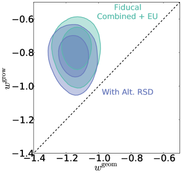
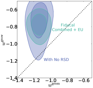
Figure 6: Dependence of our results on the RSD data and their analyses. Left panel: Combined constraints for the case where we replace the $z=0.57$ RSD measurement from Chuang et al. (2013) with the alternative BOSS measurement that uses the same raw data but a different analysis Samushia et al. (2014); see Fig. 2. The combined constraints are now only slightly less discrepant with the $w^{\rm geom}=w^{\rm grow}$ line. Right panel: Combined constraints, but without the RSD data employed. The combined contour is now larger in the growth direction; however it is still somewhat discrepant with the $w^{\rm geom}=w^{\rm grow}$ line, though less so than with the RSD data included. See text for details.

In Fig. 5, we show constraints on $w^{\text{geom}}$ and $w^{\text{grow}}$, marginalized (for each probe) over $\{\Omega_{M}^{\rm geom},\Omega_{M}^{\rm grow},\Omega_{M}h^{2},\Omega_{B}h^{2},10^{9}A,n_{s}\}$, plus the nuisance parameters as before. As in the previous case when only the matter density parameter was split, we find largely expected directions probed in this plane. However, because we now fully marginalize over the matter density parameters $\Omega_{M}^{\rm geom}$ and $\Omega_{M}^{\rm grow}$, the constraints on the equation of state are necessarily weaker. Nevertheless, BAO and SNIa still do an admirable job in constraining the geometric $w$. The CMB distance, being a single quantity, is subject to degeneracy between $\Omega_{M}^{\rm geom}$ and $w^{\rm geom}$ and, by itself, provides no constraint on either parameter alone. Finally WL and clusters also weakly constrain either equation of state parameters due to partial degeneracies. All of the aforementioned probes are broadly consistent with the $\Lambda$CDM value $w^{\mathrm{geom}}=w^{\mathrm{grow}}=-1$. In addition, we want to check that our constraints are comparable to those obtained previously. To that effect, we get constraints using only the combined CMB and weak lensing, and find that these are similar to comparible constraints obtained Wang et al. (2007) and shown in Fig. 3 of that work.

The one significant outlier are the RSD; they alone, combined with the Planck early-universe prior, precisely constrain the growth equation of state, but with the value

$$w^{\rm grow,RSD}=-0.760\pm 0.085,$$ (31)

which is clearly far from the $\Lambda$CDM value of $-1$.

The RSD data clearly pull the combined constraints away from the $w^{\rm geom}=w^{\rm grow}$ line, as a simple visual inspection of Fig. 5 shows. The fully marginalized combined constraints from all cosmological probes, including the discrepant RSD, are

$$\begin{aligned} \Omega_{M}^{\rm geom}&=0.283\pm 0.011\\[0.56917pt] \Omega_{M}^{\rm grow}&=0.311\pm 0.017\\[0.56917pt] w^{\rm geom}&=-1.13\pm 0.06\\[0.56917pt] w^{\rm grow}&=-0.77\pm 0.08\end{aligned}\qquad\mbox{($\Omega_{M}$ and $w$ both split)}$$ (32)

and those on all other parameters can be found in the last column of Table 7. Note also that the overall goodness of fit with or without RSD is satisfactory: with RSD $\chi^{2}/{\rm dof}=728/699=1.04$, while when the redshift space distortions are removed, $\chi^{2}/{\rm dof}=719/686=1.05$.

We can easily quantify the significance of the pull away from the $w^{\rm geom}=w^{\rm grow}$ line by calculating the fraction of the likelihood for $w^{\rm geom}>w^{\rm grow}$, which is the p value defined as

$$p=\frac{\int_{w^{\text{geom}}>w^{\text{grow}}}dw^{\text{geom}}dw^{\text{grow}}\mathcal{L}(w^{\text{geom}},w^{\text{grow}})}{\int dw^{\text{geom}}dw^{\text{grow}}\mathcal{L}(w^{\text{geom}},w^{\text{grow}})}.$$ (33)

The $p$-value is 0.0010 for the combined constraints, corresponding to an inconsistency with $w$CDM at $3.3\sigma$.

VI Discussion

Let us consider possible reasons for the pull of redshift-space distortions toward $w^{\rm grow}>-1$. This result is qualitatively not new: a number of recent investigations have already been established that the RSD data are in some conflict with $\Lambda$CDM, suggesting less growth at recent times than predicted by the standard model Macaulay et al. (2013). For example, Beutler et al. (2014) have measured a $>2$-$\sigma$ tension in measurements of the growth index $\gamma=0.772^{+0.124}_{-0.097}$ relative to the $\Lambda$CDM (and, for that matter, also $w$CDM) prediction $\gamma\simeq 0.55$. Similarly, Samushia et al. (2014), using DR11 CMASS sample, and the more precise results by Reid et al. (2014) that utilized smaller spatial scales by doing extensive halo occupation distribution modeling, have obtained similar results, indicating that growth is suppressed relative to $\Lambda$CDM prediction at approximately the 2-$\sigma$ level. Moreover, Beutler et al. (2014) find a $\sim$2.5$\sigma$ evidence for nonzero neutrino mass, again a signature of the hints of the departure from the standard model. Finally, Salvatelli et al. (2014) utilize the combined cosmological probes (including the RSD) in the context of a model where vacuum energy interacts with dark matter, and interpret the results as detection of nonzero interactions between dark matter and dark energy — another possible interpretation of the departure from the standard $\Lambda$CDM model.

Degeneracy with optical depth may play an important role here: our RSD measurement is combined with the early-universe prior, whose crucial input is the measurement of the optical depth to reionization $\tau$ which has been most accurately measured by WMAP’s polarization data. The higher the $\tau$, the higher the primordial fluctuation amplitude $A$ or, roughly equivalently, amplitude of mass fluctuations $\sigma_{8}$ at low redshift, and thus the larger the discrepancy. Recall from Fig. 2 that all RSD data, except perhaps the higher-redshift WiggleZ measurement, pull toward low values of $f\sigma_{8}$ relative to those predicted by the standard model. Therefore, the anomalous RSD results may perhaps partly be explained by a high WMAP-polarization estimate of $\tau$. Forthcoming Planck polarization measurements will provide more accurate constraints on the optical depth and should clarify this issue.

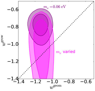
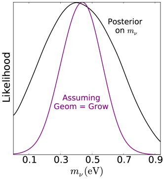
Figure 7: Left panel: The effects on the combined constraints when the sum of the neutrino masses $m_{\nu}$ is allowed to vary, compared to our fiducial assumption of holding it fixed at $0.06$ eV. The constraints are now fully consistent with the $w^{\rm geom}=w^{\rm grow}$ line. Right panel: Posterior likelihood on $m_{\nu}$ for when $\Omega_{M}$ and $w$ are split (wider curve), and when growth = geometry correspondence ($\Omega_{M}^{\rm geom}=\Omega_{M}^{\rm grow}$ and $w^{\rm geom}=w^{\rm grow}$) is enforced (narrower curve). In both cases a value of $m_{\nu}\simeq 0.45$ eV is preferred; see text for details.

Perhaps of most interest is investigating how our results depend on the choice of RSD analyses. Even within BOSS, different analyses make different assumptions and give somewhat different results; this is clearly shown for the $z=0.57$ measurements shown in Fig. 2. We do our best to avoid the a posteriori bias of hand-picking analyses that give results that are closer, or further away, from the concordance $\Lambda$CDM model. To that extent, we keep our original choice of the RSD data from Fig. 2 and Table 4 as fiducial but, as an alternative, choose to investigate what happens in the combined analysis when the measurement at $z=0.57$, which clearly is most responsible for the discrepancy with the standard model, is replaced by the alternative analysis of the same data Samushia et al. (2014). That alternative determination of $(F,f\sigma_{8})$ at $z=0.57$ is less discrepant with the $\Lambda$CDM model; see Fig. 2. The results are shown in the left panel of Fig. 6. Clearly, the combined constraints (RSD + everything else) are now slightly closer to the geometry=growth line, but the p value is still small (0.0020), indicating a 3.1-$\sigma$ discrepancy with the standard geometry=growth assumption. The constraints on cosmological parameters with the alternate RSD $z=0.57$ measurement from BOSS are

$$\begin{aligned} \Omega^{\rm geom}&=0.279\pm 0.011\\[0.56917pt] \Omega^{\rm grow}&=0.319\pm 0.021\\[0.56917pt] w^{\rm geom}&=-1.14\pm 0.06\\[0.56917pt] w^{\rm grow}&=-0.81\pm 0.08\end{aligned}\qquad\mbox{(w/ alternate RSD)}.$$ (34)

The goodness-of-fit for this case is also satisfactory, $\chi^{2}/$dof $=724/699=1.04$.

The RSD results are therefore reasonably stable with respect to the choice of data. However, while the data in the RSD analyses that we employed typically include information from large scale (roughly $10$-$30\,h^{-1}{\rm Mpc}\lesssim\sqrt{r_{\parallel}^{2}+r_{\perp}^{2}}\lesssim 150$-$200\,h^{-1}{\rm Mpc}$) — scales considered well modeled by theory — some analyses are subject to contributions from shorter scales perpendicular to the line of sight (small $r_{\perp}$), making those measurements subject to increased theory systematics Song et al. (2014). Therefore, it is prudent to be cautious in interpreting the RSD observations at this early stage.

We next investigate the implications of completely removing the RSD in the combined constraints in the right panel of Fig. 6. In this case, the combined constraints are more consistent with the geometry=growth expectations, though the p value is still somewhat small at 0.0204, corresponding to a discrepancy of 2.3$\sigma$. As mentioned earlier, the goodness-of-fit is entirely satisfactory both with and without the RSD data. Clearly, RSD currently provide by far the strongest constraint on the growth of structure.

It is also interesting to study the effect of the neutrino mass. So far, cosmology has provided rather stringent upper limits to the sum of neutrino masses, roughly $m_{\nu}\lesssim 0.3$ eV (e.g. Seljak et al., 2006). Recently several papers have claimed evidence for the positive neutrino mass in order to alleviate the discrepancy between the RSD data and the standard $\Lambda$CDM model Beutler et al. (2014), or the twin tensions between the local measurements of the expansion history and Planck data Hou et al. (2014); Dvorkin et al. (2014); Bocquet et al. (2015); Costanzi et al. (2014), and Planck and BICEP2 constraints on the amplitude of gravitational waves Dvorkin et al. (2014); Archidiacono et al. (2014).

To test the effect of neutrino mass sum on our combined constraints (including RSD), we allow it to vary within the range $m_{\nu}\in[0,1]$ eV. We compare the combined results to our fiducial case of fixing the mass sum to $m_{\nu}=0.06$ eV, the results of which can be seen in the left panel of Fig. 7. Allowing the combined masses of neutrinos to vary results in a significant increase in the range of values allowed by the combined data, and the constraints become fully consistent with the growth=geometry expectation:

$$\begin{aligned} \Omega_{M}^{\rm geom}&=0.289\pm 0.012\\[0.56917pt] \Omega_{M}^{\rm grow}&=0.319\pm 0.018\\[0.56917pt] w^{\rm geom}&=-1.11\pm 0.06\\[0.56917pt] w^{\rm grow}&=-1.10\pm 0.28\end{aligned}\quad\mbox{($m_{\nu}$ marginalized over)}.$$ (35)

Neutrino mass therefore relieves tension between geometry and growth. It is then of particular interest to report what neutrino mass sum is favored by the data. The posterior probability on $m_{\nu}$ is shown in the right panel of Fig. 7. In the case where both $\Omega_{M}$ and $w$ are split, $m_{\nu}=0.45\pm 0.21$ eV, higher than our fiducial, normal-hierarchy value (which assumes the massless lightest-mass eigenstate) of $m_{\nu}=0.06$ eV by $\sim{2}$-$\sigma$. As a further test, we place constraints on $m_{\nu}$ in the case of unsplit parameters (i.e. enforcing $\Omega_{M}^{\rm geom}=\Omega_{M}^{\rm grow}$ and $w^{\rm geom}=w^{\rm grow}$), obtaining $m_{\nu}=0.45\pm 0.12$ eV. Our results are in good agreement with Beutler et al. (2014) who favor similar neutrino mass, $m_{\nu}=0.36\pm 0.10$ eV, using the combined BAO+RSD+Planck data.

From Fig. 5 and Eq. (32) we see that the geometric equation of state is also somewhat incompatible with the $\Lambda$CDM value, since the combined data mildly prefer a value $w^{\rm geom}=-1.13\pm 0.06$. We find that most of the pull toward such negative values is provided by the BAO. The fact that $w^{\rm grow}>-1$ while $w^{\rm geom}<-1$ clearly exacerbates the disagreement between geometry and growth, leading to the 3.3$\sigma$ incompatibility calculated above; growth however clearly exhibits the more pronounced tension with the standard value.

Finally, we investigate whether there is something about the Planck early-universe prior that pushes the combined constraints away from the standard assumption that geometry=growth. To that effect, we replace the Planck prior in Table 6 with the equivalent based on WMAP nine-year data (Hinshaw et al., 2013). Runs with this prior indicate that $w^{\rm geom}=-1.13\pm 0.06$, $w^{\rm grow}=-0.78\pm 0.08$, with $w^{\rm grow}>w^{\rm geom}$ now favored at $3.1\sigma$ (p value=0.0017). These constraints with WMAP9 are very similar to those obtained with Planck, so differences between the two CMB probes’ measurements are not responsible for the tensions we observe.

VII Conclusions

In this paper we have carried out a general, weakly model-dependent test of the consistency of the $w$CDM cosmological model using current cosmological data from Type Ia supernovae, CMB peak location, baryon acoustic oscillations, redshift space distortions, cluster counts, and weak lensing. We split each late-universe parameter that describes the effects of dark energy into two parameters, one that comes from observed quantities that are governed by geometry of the cosmological model, and one that is determined by the growth of structure. Assuming flat universe, we first assume the dark energy equation of state of $-1$ and constrain the parameters determining the matter density relative to critical, $\Omega_{M}^{\rm geom}$ and $\Omega_{M}^{\rm grow}$. We then consider the case when, in addition to the matter density, the equation of state of dark energy can vary and hence $w^{\rm geom}$ and $w^{\rm grow}$ can be constrained. We marginalize over five additional early-universe parameters including the neutrino mass, plus several nuisance parameters that are specific to individual cosmological probes. As a check, we show constraints projected on popular parameter combinations $(\Omega_{M},\sigma_{8})$ and $(\Omega_{M},w)$ in Fig. 3.

The main results — constraints on the geometry and growth components of $\Omega_{M}$ and $w$ — are shown in Figs. 4 and 5, respectively. The complementarity of various probes is impressive; this is especially visually evident in the $\Omega_{M}^{\rm geom}-\Omega_{M}^{\rm grow}$ plane in Fig. 4 which shows that SNIa, BAO and CMB peak location determine distance; the remaining three probes are sensitive to both geometry and growth – RSD and cluster counts are largely sensitive to growth, while weak lensing mostly constrains the geometry. The overall goodness of fit is satisfactory, and the constraints on the late-universe parameters of interest, given in Eqs. (30) and (32) and summarized in Table 1, are very tight.

One surprise are the redshift-space distortions, which are in a $\simeq 3$-$\sigma$ conflict with $w$CDM. The RSD prefer less growth at late times than in the standard model; this can visually be seen in the RSD data — Fig. 2 shows preference for a lower $f\sigma_{8}$ than in the standard Planck $\Lambda$CDM model. The tension is most clearly seen in the $w$-split plane, Fig. 5, which shows that RSD alone prefers $w^{\rm grow,RSD}=-0.760\pm 0.085$, and in fact pulls the combined constraint from all probes to $w^{\rm grow}=-0.77\pm 0.08$. We quantify the tension with $w$CDM to be 3.3$\sigma$ (p value of $w^{\rm geom}\geq w^{\rm grow}$ is 0.0010). This tension brought about with current RSD measurements has already been noticed and discussed in the literature. In the Discussion section, we demonstrate that the discrepancy remains at the still-significant 3.1$\sigma$ level once the most discrepant RSD measurement is replaced by one from an alternative analysis. The discrepancy may be resolved with a higher value of the sum of the neutrino masses than what is expected in the normal hierarchy between the mass eigenstates with the lightest eigenstate being massless, $m_{\nu}=0.45\pm 0.12$ eV; see Fig. 7. However, systematics may play a role in resolving the discrepancy; more work in this area is needed to determine which of these effects is responsible.

On the whole, our results demonstrate very explicitly how the diverse cosmological probes complement each other and not just break degeneracy in the multidimensional parameter space, but also effectively specialize in constraining geometry, growth, or both. The resulting combined constraints on the geometry and growth are impressively tight. The next generation of surveys — Stage III and IV in the language of the Dark Energy Task Force — are sure to improve them further.

Over the past few years, as the cosmological constraints improved, we and others hoped that nature will be kind enough to provide hints for departure from the standard $\Lambda$CDM model in order to help reveal the dynamics of dark energy. We already see those hints, and it will be interesting to see whether they are cracks in the cosmic egg or perhaps systematics in data and observations.

Appendix A Cluster analysis details

Here we give more details regarding the cluster analysis, which closely followed one given in the Rozo et al. (2010) MaxBCG cosmological constraints paper.

The analysis is based on assigning “richness” to each cluster; this is defined as the number of galaxies in $R_{200}$, the radius at which the average density of the cluster is 200 times that of the critical density of the universe. Moreover, the mass is determined from richness via the richness-mass relation which has been calibrated using weak gravitational lensing measurements by Johnston et al. (2007). The cluster numbers in each richness bin are shown in Table 8, while the clusters’ mean mass per bin is shown in Table 9 and in Fig. 8.

In addition to the data in Table 8, there are also five clusters which have $N_{200}>120$. Due to the high richness of these clusters, they are not analyzed with a standard $\chi^{2}$ approach, and are instead included in the analysis on an individual basis.

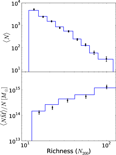
Figure 8: Top: Number of galaxy clusters within a given richness bin in the MaxBCG data set. Errors shown are the diagonal parts of the covariance matrix. The step function shown uses the parameter values from the best-fit $\Lambda$CDM model (Column 2 of Table 7). The data are summarized in Table 8. Bottom: Mean mass of galaxy clusters within the given richness bin in the MaxBCG data set. The step function uses the same parameter values as the top figure. The data are summarized in Table 9.

Richness bin	No. of Clusters
11-14	5167
14-18	2387
19-23	1504
24-29	765
30-38	533
39-48	230
49-61	134
62-78	59
79-120	31

Table 8: The number of clusters with a richness within the given bin.

Richness bin	No. of Clusters	$\langle M_{200b}\rangle[10^{14}M_{\odot}]$
12-17	5651	1.298
18-25	2269	1.983
26-40	1021	3.846
41-70	353	5.475
71+	55	13.03

Table 9: Mean mass (and their number) of clusters with a richness within the given bin.

As already implied, the overdensity of $\Delta=200$ is adopted to define cluster masses. In addition, the masses measured have been assumed to be in cosmology with $\Omega_{M}=0.27$. For other cosmologies, this leads to an overdensity of $\Delta_{v}=200(0.27/\Omega_{M})$. To correctly account for this, we rescale the quoted masses from Rozo et. al. for each tested cosmology using the equations from Hu and Kravtsov (2003) for mass rescaling

$$\frac{M_{h}}{M_{v}}=\frac{\Delta_{h}}{\Delta_{v}}\frac{1}{c^{3}}\left(\frac{r_{h}}{r_{s}}\right)^{3}$$ (36)

where $r$ is the radius of the halo for a given overdensity, $c$ the concentration factor, and $\Delta$ is the overdensity. The ratio of radii can be written as

$$\frac{r_{s}}{r_{h}}=x\left(\frac{\Delta_{v}}{\Delta_{h}}f\left(\frac{1}{c}\right)\right)$$ (37)

where

$$f(x)=x^{3}\left[\ln(1+x^{-1})-(1+x)^{-1}\right]$$ (38)

and its inverse can be approximated as

$$x(f)=\left[a_{1}f^{2p}+\left(\frac{3}{4}\right)^{2}\right]^{-1/2}+2f$$ (39)

where $p=a_{2}+a_{3}\ln f+a_{4}(\ln f)^{2}$, and $a_{i}=\{0.5116,-0.4283,-3.13\times 10^{-3},-3.52\times 10^{-5}\}$. Finally, the concentration can be expressed in terms of the mass as

$$c(M_{v})=9(1+z)^{-1}(M_{v}/M_{*})^{-0.13},$$ (40)

where $M_{*}$ is calculated at the present day.

As mentioned in Sec. III.4, the probability weighting functions are

$$\langle\psi|M\rangle =\int dN_{200}P(N_{200}|M)\psi(N_{200}),$$ (41)

$$\langle\phi|z\rangle =\int dz_{\text{photo}}P(z_{\text{photo}}|z)\phi(z_{\text{photo}}).$$ (42)

Here $P(N_{200}|M)$ is a log-normal distribution with an unknown variance $\sigma^{2}_{NM}=\text{Var}(\ln N_{200}|M)$ and an expected value

$$\langle\ln N_{200}|M\rangle=$$ (43)

$$\frac{\log_{10}\left(\frac{M}{M_{1}}\right)\langle\ln N_{200}|M_{2}\rangle-\log_{10}\left(\frac{M}{M_{2}}\right)\langle\ln N_{200}|M_{1}\rangle}{\log_{10}\left(\frac{M_{2}}{M_{1}}\right)}$$

where $M_{1}=1.3\times 10^{14}M_{\odot}$, $M_{2}=1.3\times 10^{15}M_{\odot}$, and $\langle\ln N_{200}|M_{1}\rangle$, $\langle\ln N_{200}|M_{2}\rangle$, and $\sigma^{2}_{NM}$ are nuisance parameters, which are marginalized over during the analysis of the cluster data. Likewise, the probability weighting function $P(z_{\text{photo}}|z)$ is a Gaussian distribution with standard deviation $\sigma_{z}=0.008$ and an expectation value $\langle z_{\text{photo}}|z\rangle=z$. $\psi(N_{200})$ and $\phi(z_{\text{photo}})$ are once again binning functions, where the $z_{\text{photo}}$ bin is $[0.1,0.3]$ from the range of photometric data from the SDSS survey.

The cluster likelihood consists of two parts Rozo et al. (2010); the main part is defined via

$$-2\log\mathcal{L_{\text{main}}}=\Delta x^{\text{T}}C^{-1}\Delta x$$ (44)

where $\Delta x=(x^{\text{data}}-x^{\text{theory}})$. The x vector of observables is

$$x=\{N_{1},...,N_{9},(N\bar{M})_{1},...,(N\bar{M})_{5}\}.$$ (45)

where $N_{1}$ though $N_{9}$ are the cluster counts in the respective richness bins, while $(N\bar{M})_{1}$ through $(N\bar{M})_{5}$ are the total mass of clusters in bins.

The covariance $C$ of the cluster data takes into account uncertainties due to shot noise, sample variance, the stochasticity of the mass-richness relation, measurement error of the weak lensing masses, and uncertainties in the purity and completeness of the sample. For more information regarding these uncertainties, see Rozo et al. (2010) from which we adopt the prescription for calculating the covariance matrix.

As previously stated, there are five clusters in the MaxBCG data set which have $N_{200}=126$, $139$, $156$, $164$, and $188$. These clusters are added on a individual basis to the analysis with the likelihood

$$\log\mathcal{L_{\text{tail}}}=\sum_{N_{200}>120}\langle N\rangle-\sum_{N(N_{200})=1}\langle N\rangle+\log\langle N\rangle$$ (46)

where the first sum is over all richnesses $>120$, which is subtracted by the second sum, which is for those richness bins that contain a cluster. This additional piece is combined with the main part to obtain the full likelihood of observing a set of cluster counts and their masses

$$\mathcal{L}_{\text{cluster}}=\mathcal{L}_{\text{main}}\mathcal{L}_{\text{tail}}.$$ (47)

Appendix B RSD analysis details

B.1 RSD correlation matrices

For completeness, in Tables 10 and 11 we present the correlation matrices for the BOSS Low-$z$, BOSS CMASS, and WiggleZ measurements used for the analysis. The square roots of the diagonal uncertainties for these measurements can be found in Table 4.

$z=0.32$	$H(z)$	$D_{A}(z)$	$f\sigma_{8}$
$H(z)$	$1.00$	$-0.32$	$0.35$
$D_{A}(z)$	—	$1.00$	$0.51$
$f\sigma_{8}$	—	—	$1.00$

$z=0.57$	$H(z)$	$D_{A}(z)$	$f\sigma_{8}$
$H(z)$	$1.00$	$-0.67$	$0.05$
$D_{A}(z)$	—	$1.00$	$0.40$
$f\sigma_{8}$	—	—	$1.00$

Table 10: Correlation matrices for the BOSS Low-z (left) and CMASS (right) samples of our RSD data set.

	$F_{a}$	$F_{b}$	$F_{c}$	$(f\sigma_{8})_{a}$	$(f\sigma_{8})_{b}$	$(f\sigma_{8})_{c}$
$F_{a}$	$1.00$	$0.52$	$0.00$	$0.73$	$0.35$	$0.00$
$F_{b}$	—	$1.00$	$0.50$	$0.38$	$0.74$	$0.43$
$F_{c}$	—	—	$1.00$	$0.00$	$0.43$	$0.85$
$(f\sigma_{8})_{a}$	—	—	—	$1.00$	$0.51$	$0.00$
$(f\sigma_{8})_{b}$	—	—	—	—	$1.00$	$0.56$
$(f\sigma_{8})_{c}$	—	—	—	—	—	$1.00$

Table 11: Correlation matrix for the WiggleZ sample of our RSD data set. Terms with subscript $a$ are values at $z=0.44$, subscript $b$ at $z=0.60$, and subscript $c$ at $z=0.73$.

B.2 From $(D_{A},H)$ covariance to error in $F$

In order to make the error bars in Fig. 2 for the two BOSS samples (Low-z and CMASS), we need to project the $3\times 3$ covariance matrix in $f\sigma_{8}$, $H$ and $D_{A}$ into the $2\times 2$ space $(f\sigma_{8},F)$. Recall, $F$ is defined in Eq. (22) and is essentially proportional to the product of the Hubble parameter and the angular diameter distance.

Doing this is a short exercise in statistics. First of all, note that we only really need the variance in $F$, although computing the covariance between $f\sigma_{8}$ and $F$ would be equally straightforward.

Let us assume that we would like to calculate the variance of the product of two Gaussian random variables $x$ and $y$. Let $X$ and $Y$ be the mean of these two variables, and $\delta x\equiv x-X$ and $\delta y\equiv y-Y$. Then

$${\rm Var}(xy) ={\rm Var}[(X+\delta x)(Y+\delta y)]$$ (48)

$$={\rm Var}[X\delta y+Y\delta x+\delta x\delta y]$$

where we dropped the noncontributing variance of a constant. Dropping the three-point correlations that vanish for Gaussian variables, this evaluates to where in the last expression we evaluated ${\rm Var}(\delta x\delta y)$ using Wick’s theorem. This is the expression that we need. Denoting for clarity $D_{A}$ and $H$ to be the means, and $\mathcal{D}_{A}$ and $\mathcal{H}$ to be fluctuations around the mean in the angular diameter distance and Hubble parameter, in our case we have

$$(1+z)^{-2}{\rm Var}(F) = H^{2}{\rm Var}(\mathcal{D}_{A})+D_{A}^{2}{\rm Var}(\mathcal{H})$$

$$+ 2HD_{A}{\rm Cov}(\mathcal{D}_{A},\mathcal{H})$$

$$+ {\rm Var}(\mathcal{D}_{A}){\rm Var}(\mathcal{H})+{\rm Cov}(\mathcal{D}_{A},\mathcal{H})^{2}.$$

With this equation we can evaluate the error in $F$, given the covariance matrix in the angular diameter distance and Hubble parameter.

Appendix C Plots with separated contours

In Figs. 9, 10, and 11, and 12, we include alternate versions of Figs. 3(a), 3(b), 4, and 5. Here, for clarity, each probe’s constraints have been shown separately. In each case, the combined constraint has also been shown.

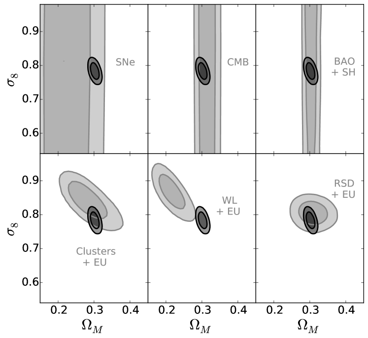
Figure 9: Same as the left panel of Fig. 3, but the various probes have been separated for easier viewing. The smaller, dark set of contours corresponds to all probes combined.

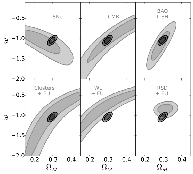
Figure 10: Same as the right panel of Fig. 3, but the various probes have been separated for easier viewing. The smaller, dark set of contours corresponds to all probes combined.

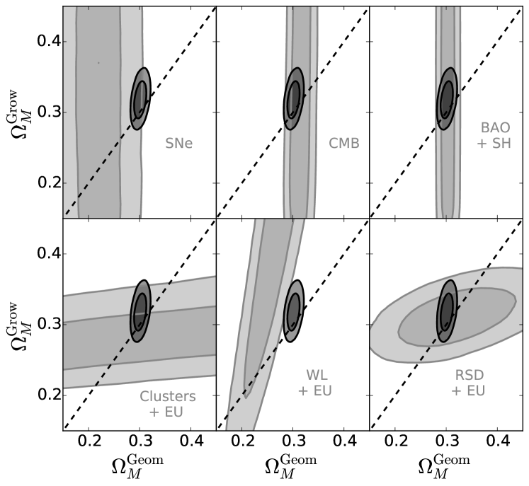
Figure 11: Same as Fig. 4, but the various probes have been separated for easier viewing. The smaller, dark set of contours corresponds to all probes combined.

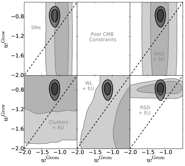
Figure 12: Same as Fig. 5, but the various probes have been separated for easier viewing. The smaller, dark set of contours corresponds to all probes combined.

References

- Riess et al. (1998) A. G. Riess et al., Astron. J. 116, 1009 (1998), astro-ph/9805201 .
- Perlmutter et al. (1999) S. Perlmutter et al., Astrophys. J. 517, 565 (1999), astro-ph/9812133 .
- Frieman et al. (2008) J. Frieman, M. Turner, and D. Huterer, Ann.Rev.Astron.Astrophys. 46, 385 (2008), arXiv:0803.0982 [astro-ph] .
- Joyce et al. (2015) A. Joyce, B. Jain, J. Khoury, and M. Trodden, Phys.Rept. 568, 1 (2015), arXiv:1407.0059 [astro-ph.CO] .
- Ishak et al. (2006) M. Ishak, A. Upadhye, and D. N. Spergel, Phys.Rev. D74, 043513 (2006), arXiv:astro-ph/0507184 [astro-ph] .
- Zhan et al. (2009) H. Zhan, L. Knox, and J. A. Tyson, Astrophys.J. 690, 923 (2009), arXiv:0806.0937 [astro-ph] .
- Mortonson et al. (2009) M. J. Mortonson, W. Hu, and D. Huterer, Phys.Rev. D79, 023004 (2009), arXiv:0810.1744 [astro-ph] .
- Mortonson et al. (2010) M. J. Mortonson, W. Hu, and D. Huterer, Phys.Rev. D81, 063007 (2010), arXiv:0912.3816 [astro-ph.CO] .
- Acquaviva and Gawiser (2010) V. Acquaviva and E. Gawiser, Phys.Rev. D82, 082001 (2010), arXiv:1008.3392 [astro-ph.CO] .
- Vanderveld et al. (2012) R. A. Vanderveld, M. J. Mortonson, W. Hu, and T. Eifler, Phys.Rev. D85, 103518 (2012), arXiv:1203.3195 [astro-ph.CO] .
- Zhao et al. (2010) G.-B. Zhao, T. Giannantonio, L. Pogosian, A. Silvestri, D. J. Bacon, et al., Phys.Rev. D81, 103510 (2010), arXiv:1003.0001 [astro-ph.CO] .
- Bean and Tangmatitham (2010) R. Bean and M. Tangmatitham, Phys.Rev. D81, 083534 (2010), arXiv:1002.4197 [astro-ph.CO] .
- Zhao et al. (2012) G.-B. Zhao, H. Li, E. V. Linder, K. Koyama, D. J. Bacon, et al., Phys.Rev. D85, 123546 (2012), arXiv:1109.1846 [astro-ph.CO] .
- Hojjati et al. (2012) A. Hojjati, G.-B. Zhao, L. Pogosian, A. Silvestri, R. Crittenden, et al., Phys.Rev. D85, 043508 (2012), arXiv:1111.3960 [astro-ph.CO] .
- Dossett et al. (2011a) J. Dossett, J. Moldenhauer, and M. Ishak, Phys.Rev. D84, 023012 (2011a), arXiv:1103.1195 [astro-ph.CO] .
- Dossett et al. (2011b) J. N. Dossett, M. Ishak, and J. Moldenhauer, Phys.Rev. D84, 123001 (2011b), arXiv:1109.4583 [astro-ph.CO] .
- Silvestri et al. (2013) A. Silvestri, L. Pogosian, and R. V. Buniy, Phys.Rev. D87, 104015 (2013), arXiv:1302.1193 [astro-ph.CO] .
- Wang et al. (2007) S. Wang, L. Hui, M. May, and Z. Haiman, Phys.Rev. D76, 063503 (2007), arXiv:0705.0165 [astro-ph] .
- Zhang et al. (2005) J. Zhang, L. Hui, and A. Stebbins, Astrophys.J. 635, 806 (2005), arXiv:astro-ph/0312348 [astro-ph] .
- Chu and Knox (2005) M. Chu and L. Knox, Astrophys.J. 620, 1 (2005), arXiv:astro-ph/0407198 [astro-ph] .
- Abate and Lahav (2008) A. Abate and O. Lahav, MNRAS 389, L47 (2008), arXiv:0805.3160 .
- Krauss and Turner (1995) L. M. Krauss and M. S. Turner, Gen.Rel.Grav. 27, 1137 (1995), arXiv:astro-ph/9504003 [astro-ph] .
- Scolnic et al. (2014) D. Scolnic, A. Rest, A. Riess, M. Huber, R. Foley, et al., Astrophys.J. 795, 45 (2014), arXiv:1310.3824 [astro-ph.CO] .
- Cheng and Huang (2014) C. Cheng and Q.-G. Huang, Phys.Rev. D89, 043003 (2014), arXiv:1306.4091 [astro-ph.CO] .
- Xia et al. (2013) J.-Q. Xia, H. Li, and X. Zhang, Phys.Rev. D88, 063501 (2013), arXiv:1308.0188 [astro-ph.CO] .
- Shafer and Huterer (2014) D. L. Shafer and D. Huterer, Phys.Rev. D89, 063510 (2014), arXiv:1312.1688 [astro-ph.CO] .
- Linder (2005) E. V. Linder, Phys. Rev. D72, 043529 (2005), astro-ph/0507263 .
- Conley et al. (2011) A. Conley et al. (SNLS Collaboration), Astrophys.J.Suppl. 192, 1 (2011), arXiv:1104.1443 [astro-ph.CO] .
- Ruiz et al. (2012) E. J. Ruiz, D. L. Shafer, D. Huterer, and A. Conley, Phys.Rev. D86, 103004 (2012), arXiv:1207.4781 [astro-ph.CO] .
- Frieman et al. (2003) J. A. Frieman, D. Huterer, E. V. Linder, and M. S. Turner, Phys.Rev. D67, 083505 (2003), arXiv:astro-ph/0208100 [astro-ph] .
- Zahn and Zaldarriaga (2003) O. Zahn and M. Zaldarriaga, Phys.Rev. D67, 063002 (2003), arXiv:astro-ph/0212360 [astro-ph] .
- Ade et al. (2014) P. Ade et al. (Planck Collaboration), Astron.Astrophys. (2014), 10.1051/0004-6361/201321591, arXiv:1303.5076 [astro-ph.CO] .
- Eisenstein et al. (2005) D. J. Eisenstein et al. (SDSS Collaboration), Astrophys.J. 633, 560 (2005), arXiv:astro-ph/0501171 [astro-ph] .
- Beutler et al. (2011) F. Beutler, C. Blake, M. Colless, D. H. Jones, L. Staveley-Smith, et al., Mon.Not.Roy.Astron.Soc. 416, 3017 (2011), arXiv:1106.3366 [astro-ph.CO] .
- Padmanabhan et al. (2012) N. Padmanabhan, X. Xu, D. J. Eisenstein, R. Scalzo, A. J. Cuesta, et al., Mon.Not.Roy.Astron.Soc. 427, 2132 (2012), arXiv:1202.0090 [astro-ph.CO] .
- Anderson et al. (2012) L. Anderson, E. Aubourg, S. Bailey, D. Bizyaev, M. Blanton, et al., Mon.Not.Roy.Astron.Soc. 427, 3435 (2012), arXiv:1203.6594 [astro-ph.CO] .
- Eisenstein and Hu (1999) D. J. Eisenstein and W. Hu, Astrophys.J. 511, 5 (1999), arXiv:astro-ph/9710252 [astro-ph] .
- Allen et al. (2011) S. W. Allen, A. E. Evrard, and A. B. Mantz, Ann.Rev.Astron.Astrophys. 49, 409 (2011), arXiv:1103.4829 [astro-ph.CO] .
- Rozo et al. (2010) E. Rozo et al. (DSDD Collaboration), Astrophys.J. 708, 645 (2010), arXiv:0902.3702 [astro-ph.CO] .
- Koester et al. (2007) B. Koester et al. (SDSS Collaboration), Astrophys.J. 660, 239 (2007), arXiv:astro-ph/0701265 [astro-ph] .
- Johnston et al. (2007) D. E. Johnston et al. (SDSS Collaboration), (2007), arXiv:0709.1159 [astro-ph] .
- Tinker et al. (2008) J. L. Tinker, A. V. Kravtsov, A. Klypin, K. Abazajian, M. S. Warren, et al., Astrophys.J. 688, 709 (2008), arXiv:0803.2706 [astro-ph] .
- Erben et al. (2013) T. Erben, H. Hildebrandt, L. Miller, L. van Waerbeke, Heymans, et al., MNRAS 433, 2545 (2013), arXiv:1210.8156 [astro-ph.CO] .
- Heymans et al. (2012) C. Heymans, L. Van Waerbeke, L. Miller, T. Erben, Hildebrandt, et al., MNRAS 427, 146 (2012), arXiv:1210.0032 [astro-ph.CO] .
- Huterer and Takada (2005) D. Huterer and M. Takada, Astroparticle Physics 23, 369 (2005), astro-ph/0412142 .
- Smith et al. (2003) R. E. Smith, J. A. Peacock, A. Jenkins, S. D. M. White, C. S. Frenk, F. R. Pearce, P. A. Thomas, G. Efstathiou, and H. M. P. Couchman, MNRAS 341, 1311 (2003), astro-ph/0207664 .
- Takahashi et al. (2012) R. Takahashi, M. Sato, T. Nishimichi, A. Taruya, and M. Oguri, Astrophys.J. 761, 152 (2012), arXiv:1208.2701 [astro-ph.CO] .
- Samushia et al. (2014) L. Samushia, B. A. Reid, M. White, W. J. Percival, A. J. Cuesta, et al., Mon.Not.Roy.Astron.Soc. 439, 3504 (2014), arXiv:1312.4899 [astro-ph.CO] .
- Jackson (1972) J. C. Jackson, MNRAS 156, 1P (1972).
- Song and Percival (2009) Y.-S. Song and W. J. Percival, JCAP 0910, 004 (2009), arXiv:0807.0810 [astro-ph] .
- Ballinger et al. (1996) W. Ballinger, J. Peacock, and A. Heavens, Mon.Not.Roy.Astron.Soc. 282, 877 (1996), arXiv:astro-ph/9605017 [astro-ph] .
- Matsubara and Suto (1996) T. Matsubara and Y. Suto, Astrophys.J. 470, L1 (1996), arXiv:astro-ph/9604142 [astro-ph] .
- Simpson and Peacock (2010) F. Simpson and J. A. Peacock, Phys.Rev. D81, 043512 (2010), arXiv:0910.3834 [astro-ph.CO] .
- Alcock and Paczynski (1979) C. Alcock and B. Paczynski, Nature 281, 358 (1979).
- Beutler et al. (2012) F. Beutler, C. Blake, M. Colless, D. H. Jones, L. Staveley-Smith, et al., Mon.Not.Roy.Astron.Soc. 423, 3430 (2012), arXiv:1204.4725 [astro-ph.CO] .
- Chuang et al. (2013) C.-H. Chuang, F. Prada, F. Beutler, D. J. Eisenstein, S. Escoffier, et al., (2013), arXiv:1312.4889 [astro-ph.CO] .
- Blake et al. (2012) C. Blake, S. Brough, M. Colless, C. Contreras, W. Couch, et al., Mon.Not.Roy.Astron.Soc. 425, 405 (2012), arXiv:1204.3674 [astro-ph.CO] .
- Beringer et al. (2012) J. Beringer et al. (Particle Data Group), Phys.Rev. D86, 010001 (2012).
- Gelman and Rubin (1992) A. Gelman and D. Rubin, Statistical Science 7, 457 (1992), http://www.stat.columbia.edu/~gelman/research/published/itsim.pdf.
- MacCrann et al. (2014) N. MacCrann, J. Zuntz, S. Bridle, B. Jain, and M. R. Becker, (2014), arXiv:1408.4742 [astro-ph.CO] .
- Macaulay et al. (2013) E. Macaulay, I. K. Wehus, and H. K. Eriksen, Phys.Rev.Lett. 111, 161301 (2013), arXiv:1303.6583 [astro-ph.CO] .
- Beutler et al. (2014) F. Beutler, S. Saito, H.-J. Seo, J. Brinkmann, K. S. Dawson, et al., MNRAS 443, 1065 (2014), arXiv:1312.4611 .
- Reid et al. (2014) B. A. Reid, H.-J. Seo, A. Leauthaud, J. L. Tinker, and M. White, MNRAS 444, 476 (2014), arXiv:1404.3742 .
- Beutler et al. (2014) F. Beutler et al. (BOSS Collaboration), Mon.Not.Roy.Astron.Soc. 444, 3501 (2014), arXiv:1403.4599 [astro-ph.CO] .
- Salvatelli et al. (2014) V. Salvatelli, N. Said, M. Bruni, A. Melchiorri, and D. Wands, Phys.Rev.Lett. 113, 181301 (2014), arXiv:1406.7297 [astro-ph.CO] .
- Song et al. (2014) Y.-S. Song, C. G. Sabiu, T. Okumura, M. Oh, and E. V. Linder, JCAP 1412, 005 (2014), arXiv:1407.2257 [astro-ph.CO] .
- Seljak et al. (2006) U. Seljak, A. Slosar, and P. McDonald, JCAP 0610, 014 (2006), arXiv:astro-ph/0604335 [astro-ph] .
- Hou et al. (2014) Z. Hou, C. Reichardt, K. Story, B. Follin, R. Keisler, et al., Astrophys.J. 782, 74 (2014), arXiv:1212.6267 [astro-ph.CO] .
- Dvorkin et al. (2014) C. Dvorkin, M. Wyman, D. H. Rudd, and W. Hu, Phys.Rev. D90, 083503 (2014), arXiv:1403.8049 [astro-ph.CO] .
- Bocquet et al. (2015) S. Bocquet et al. (SPT Collaboration), Astrophys.J. 799, 214 (2015), arXiv:1407.2942 [astro-ph.CO] .
- Costanzi et al. (2014) M. Costanzi, B. Sartoris, M. Viel, and S. Borgani, JCAP 1410, 081 (2014), arXiv:1407.8338 [astro-ph.CO] .
- Archidiacono et al. (2014) M. Archidiacono, N. Fornengo, S. Gariazzo, C. Giunti, S. Hannestad, et al., JCAP 1406, 031 (2014), arXiv:1404.1794 [astro-ph.CO] .
- Hinshaw et al. (2013) G. Hinshaw et al. (WMAP), Astrophys.J.Suppl. 208, 19 (2013), arXiv:1212.5226 [astro-ph.CO] .
- Hu and Kravtsov (2003) W. Hu and A. V. Kravtsov, Astrophys.J. 584, 702 (2003), arXiv:astro-ph/0203169 [astro-ph] .