Li intercalation in graphite: a van der Waals density functional study

Abstract

Modeling layered intercalation compounds from first principles poses a problem, as many of their properties are determined by a subtle balance between van der Waals interactions and chemical or Madelung terms, and a good description of van der Waals interactions is often lacking. Using van der Waals density functionals we study the structures, phonons and energetics of the archetype layered intercalation compound Li-graphite. Intercalation of Li in graphite leads to stable systems with calculated intercalation energies of $-0.2$ to $-0.3$ eV/Li atom, (referred to bulk graphite and Li metal). The fully loaded stage 1 and stage 2 compounds LiC₆ and Li_1/2C₆ are stable, corresponding to two-dimensional $\sqrt{3}\times\sqrt{3}$ lattices of Li atoms intercalated between two graphene planes. Stage $N>2$ structures are unstable compared to dilute stage 2 compounds with the same concentration. At elevated temperatures dilute stage 2 compounds easily become disordered, but the structure of Li_3/16C₆ is relatively stable, corresponding to a $\sqrt{7}\times\sqrt{7}$ in-plane packing of Li atoms. First-principles calculations, along with a Bethe-Peierls model of finite temperature effects, allow for a microscopic description of the observed voltage profiles.

I Introduction

Intercalation of metal atoms into graphiteDresselhaus and Dresselhaus (2002) has lead to a wealth of interesting physical phenomena. Alkali, alkaline earth or rare earth metal atoms can be inserted between the graphene layers of graphite without disrupting the bonding pattern within the graphene layers, and the electronic structure of the metal-graphite compound can be deduced from the interactions between the graphene and the metal layers.Pan et al. (2011); Csanyi et al. (2005) Intercalation in few-layer graphene is explored for modifying its electronic, transport, and optical properties.Petrović et al. (2013); Bao et al. (2014) Some of these metal-graphite compounds even become superconducting.Weller et al. (2005); Pan et al. (2011); Cabaret et al. (2013) The metal intercalation process is usually reversible, making graphitic carbon one of the most used materials in anodes of rechargeable batteries.Dahn et al. (1995); Winter et al. (1998); Endo et al. (2000); Kaskhedikar and Maier (2009)

Li-graphite is the archetypical intercalation compound in this class, whose composition Li_xC₆ can easily be varied between $x=0$ and $x=1$, giving rise to a surprisingly rich phase diagram.Dahn (1991); Ohzuku et al. (1993); Senyshyn et al. (2013); Billaud et al. (1996); Reynier et al. (2004); Chevallier et al. (2013) Li intercalation in carbon-based materials is also relevant to hydrogen storage, as a tool to manipulate dehydrogenation reactions.Gross et al. (2008); Ngene et al. (2010); Liu et al. (2011); Hazrati et al. (2014) The structure of the fully loaded stage 1 compound LiC₆ consists of graphene alternating with a layer of Li atoms. Controlling the Li content electrochemically and monitoring the Li_xC₆ potential as a function of $x$ shows a sequence of plateaus that is interpreted as subsequent phase equilibria.Dahn (1991); Ohzuku et al. (1993); Senyshyn et al. (2013); Billaud et al. (1996); Reynier et al. (2004); Chevallier et al. (2013) Stage $N$ ($=2,3,...$) defines a structure consisting of a stack of $N$ graphene layers alternating with a Li layer,Dresselhaus and Dresselhaus (2002) and for $1/N<x<1/(N-1)$ it is proposed that the stage $N$ and stage $N-1$ phases are in equilibrium. Upon decreasing the Li content to $x<1/N$, one then moves to the next equilibrium plateau between stage $N+1$ and stage $N$ phases. This simple model is under scrutiny though, as neutron diffraction experiments give evidence for the formation of phases with partially filled Li layers instead of fully completed higher order stage $N$ phases,Senyshyn et al. (2013) and calculations suggest the relative stability of certain partially filled structures.Filhol et al. (2008)

Experimental characterization of Li intercalation is hampered by kinetic barriers,Langer et al. (2013) which can give rise to non-equilibrium intermediate phases. First-principles calculations provide a valuable contribution to modeling the intercalation process,Bhattacharya and Van der Ven (2011); Morgan and Madden (2012) but specifically for the prototype intercalation compound Li-graphite this has proven to be a challenging task. Different Li-graphite phases emerge from a subtle balance between the interactions of the Li atoms with the graphene sheets and the van der Waals (vdW) interactions between the graphene sheets.Persson et al. (2010) The most widely used first-principles approaches, i.e. localKohn and Sham (1965) or semi-local approximationsPerdew et al. (1996) to density functional theory (DFT),Hohenberg and Kohn (1964) fail to describe the inherently non-local vdW interactions.

The phase diagram of Li-graphite based upon calculations with a semi-local functional, without correcting for vdW interactions, is even qualitatively wrong, as it does not yield any particularly stable ordered structure besides the stage 1 compound LiC₆, which is in contradiction to experimental results.Dahn (1991); Ohzuku et al. (1993); Senyshyn et al. (2013); Billaud et al. (1996); Reynier et al. (2004); Chevallier et al. (2013) Although it does not include vdW interactions, the local density approximation (LDA) yields reasonable equilibrium structures, both for graphite, as well as for the stage 1 intercalation compound LiC₆.Kganyaga and Ngoepe (2003); Could et al. (2013) As we will discuss below, the energetics of intercalation is not described very accurately by LDA however. The interlayer binding energy of graphite is a factor of two too small, whereas the Li intercalation energy is a factor of two too large.

One may include vdW interactions by adding a parametrized semi-empirical atom-atom dispersion energy to the conventional Kohn-Sham DFT energy, as in the DFT-D2 method.Grimme (2006) A problem with this approach is that vdW interactions depend critically on the charge state of the atoms involved. For instance, the vdW interaction of a Li⁺ ion with its environment is substantially smaller than that of the neutral Li atom (because virtual excitations from the 2s shell give a large contribution to the polarizability of the atom and the vdW interaction). As Li atoms interacting with graphene become partially ionized,Er et al. (2009) the parameters describing the vdW interaction need to be refitted.Lee and Persson (2012) This means that the method loses its predictive power if the charge on the metal atoms is not known beforehand. Other semi-empirical schemes have been developed that are specifically targeted at modeling vdW interactions in layered materials such as graphite, requiring the input of the material’s elastic properties, obtained either from advanced many-body calculations, or from experiment.Could et al. (2013)

Many-body approaches such as quantum Monte Carlo (QMC) or the random phase approximation (ACFDT-RPA) incorporate a description of the vdW interactions, and have been used to calculate the binding between the graphene layers in graphite, for instance.Spanu et al. (2009); Lebègue et al. (2010) However, as such methods are computationally very demanding, they cannot be applied to Li-graphite compositions that require the use of large unit cells. An alternative approach to include vdW interactions is using a van der Waals density functional (vdW-DF),Rydberg et al. (2000, 2003); Dion et al. (2004); Thonhauser et al. (2007) which is an explicit non-local functional of the density. This is the approach we use here.

In this paper we study the intercalation of Li into graphite entirely from first-principles using a vdW DFT functional, i.e., without any empirical data or ad hoc vdW corrections. First we validate this approach by calculations on pure graphite. In particular we show that the phonon band structure and elastic constants of graphite are reproduced well, including the ones that depend on the coupling between the graphene layers, where the contribution of vdW interactions is critical. Then we apply this approach to intercalation compounds Li_xC₆, $0\leq x\leq 1$, identifying stable phases and their properties. We establish that the fully loaded stage 1 and stage 2 compounds are stable, but stage $N>2$ structures are unstable compared to dilute stage 2 compounds with the same concentration. At elevated temperatures these dilute stage 2 compounds easily become disordered.

This paper is organized as follows. Sec. II discusses the computational details. In Sec. III.1 we apply the vdW-DF approach to bulk graphite and compare the performance of different versions of the vdW-DF. In Sec. III.2 we study the Li intercalation into graphite, and Sec. IV presents the summary and conclusions.

II Computational Methods

We perform first-principles calculations within the framework of density functional theory (DFT)Hohenberg and Kohn (1964); Kohn and Sham (1965) using the projector augmented wave method (PAW)Blöchl (1994); Kresse and Joubert (1999) as implemented in the Vienna ab initio simulation package (VASP).Kresse and Furthmüller (1996a, b) To include the non-local vdW interactions, we use a van der Waals density functional Dion et al. (2004); Thonhauser et al. (2007) as implemented in VASPKlimeš et al. (2010, 2011) using the algorithm of Ref. Román-Pérez and Soler, 2009. The exchange-correlation energy in the vdW-DF has the form

$$E_{\rm xc}=E_{\rm x}+[E_{\rm c}{\rm(vdW)}+E_{\rm c}{\rm(loc)}],$$ (1)

where $E_{\rm c}{\rm(vdW)}$ is the energy resulting from non-local electron-electron correlations, approximated by an expression in terms of the electron density, Dion et al. (2004); Thonhauser et al. (2007) and $E_{\rm c}{\rm(loc)}$ represents the energy contribution of the local electron-electron correlations, for which the local density approximation (LDA) is used. In the original vdW-DF,Dion et al. (2004) the revPBE functionalZhang and Yang (1998) is used to calculate the contribution of the exchange energy $E_{\rm x}$. We also try the vdW-DF2 functional,Lee et al. (2010) which uses a modified vdW kernel along with the PW86 exchange functional.Perdew and Wang (1986) Both the original vdW-DF and the vdW-DF2 functionals tend to overestimate the lattice constants and underestimate the formation energies of solids somewhat.Klimeš et al. (2011) The optimized exchange functionals introduced in Refs. Klimeš et al., 2010 and Klimeš et al., 2011, i.e. optB88, optPBE and optB86b, alleviate these problems, and we will test these functionals.

Standard PAW data sets are used, which are generated and unscreened using the PBE functional.Perdew et al. (1996) For lithium we use an all-electron PAW description, whereas for carbon the 1s core state is kept frozen. A kinetic energy cutoff of 550 eV is employed for the plane wave expansion of the Kohn-Sham states. The atomic positions are optimized with the conjugate gradient method until the forces on atoms are less than 10^-2 eV/Å. This criterion is sufficiently strict to obtain converged total energies. In addition to atomic positions, the volume and shape of the cells are optimized for bulk graphite and the Li-graphite compounds.not

Lattice vibrational frequencies are calculated for bulk graphite and the Li-graphite systems from the dynamical matrix, where the force constants are obtained using the finite difference method of Ref. Kresse et al., 1995. Calculating an accurate dynamical matrix requires starting from very accurate atomic equilibrium positions. So as a first step the latter are further optimized until the forces on the atoms are less than 10^-4 eV/Å. Next the atoms are displaced one-by-one and the resulting forces on all the other atoms are calculated. The typical size of a displacement is $n\times 0.015$ Å. Four displacements ($n=\{-2,-1,1,2\}$) per independent degree-of-freedom are applied in order to remove anharmonic contributions to the forces.

A $\Gamma$-centered 24$\times$24$\times$10 $k$-point mesh is used to sample the Brillouin zone (BZ) of AB stacked graphite. The same $k$-point density is used for the calculations on Li intercalation in graphite. The Methfessel-Paxton (MP) schemeMethfessel and Paxton (1989) with a smearing width of 0.2 eV is employed for the occupation of the electronic levels. The energy convergence with respect to the $k$-point sampling is better than 1 meV/C.

III Results

Table 1: The equilibrium in-plane lattice constant $a$, interlayer distance $d$ and interlayer binding energy $E_{\rm B}$ of graphite calculated using different exchange and correlation functionals, compared to experiment (Exp.) and to results from many body wave function calculations (ACFDT-RPA, QMC).

Exchange	PBE	PBE	optB88	optPBE	optB86b	revPBE	rPW86	ACFDT-RPA	QMC	Exp.
Correlation	PBE	vdW+LDA	vdW+LDA	vdW+LDA	vdW+LDA	vdW+LDA	vdW2+LDA
$a$(Å)	2.47	2.47	2.47	2.48	2.47	2.48	2.48			2.46
$d$(Å)	4.40	3.44	3.36	3.44	3.31	3.59	3.51	3.34	3.43	3.34
$E_{\rm B}$(meV/C)	1.0	70.8	69.5	63.7	69.9	52.7	52.0	48	56$\pm$5	52$\pm$5

III.1 Graphite

We start with bulk graphite to critically test different vdW-DFs. Key quantities are the equilibrium structure and the equilibrium binding energy. Somewhat more demanding properties that probe the potential energy surface close the equilibrium minimum, are the phonon spectrum and the elastic constants. Table 1 gives the equilibrium distance $d$ between the graphene layers and the equilibrium interlayer binding energy $E_{\rm B}$ (the graphite total energy subtracted from twice the total energy of isolated graphene layers), calculated using different exchange and vdW functionals. All tested functionals yield an in-plane lattice constant $a$ very close to the experimental value, indicating that the binding within a graphene plane is represented well. The interlayer distance $d$, however, is considerably overestimated by plain PBE without vdW forces (PBE-PBE): 4.40 Å vs. 3.34 Å. Indeed, the lack of vdW attraction is also apparent from a near absence of any interlayer binding ($E_{\rm B}=1$ meV/C). LDA gives a reasonable interlayer distance of 3.25Å, but a interlayer binding of only 24 meV.Kganyaga and Ngoepe (2003); Could et al. (2013); Spanu et al. (2009); Lebègue et al. (2010)

By including vdW interactions both the interlayer distance and binding energy are reproduced markedly better. There is a modest spread in the results produced by the different functionals. The optB88-vdW and optB86b-vdW functionals give the best performance regarding the structure, with optimized interlayer distances within 1% of the experimental value (3.34 Å). The PBE-vdW and optPBE-vdW functionals give interlayer distances that are 3% too large, and the interlayer distances produced by the revPBE-vdW and rPW86-vdW2 functionals are 5% and 7.5% too large, respectively. Concerning performance with regard to binding energy, the order of the functionals is reversed. The revPBE-vdW and rPW86-vdW2 functionals give a binding energy that is very close to the experimental value and to the value obtained from quantum Monte Carlo calculations (QMC).Spanu et al. (2009) The other functionals (PBE-vdW, optB88-vdW, optPBE-vdW and optB86b-vdW) overestimate the experimental binding energy by 21 to 24 $\%$. These results are in line with previous findings.Hamada and Otani (2010); Mapasha et al. (2012); Graziano et al. (2012)

From here on we select the optB88-vdW functional for our calculations, as it gives a very good interlayer distance and an acceptable interlayer binding energy. Details of the graphite structure are also given correctly. For instance, AB-stacked graphite is 10 meV/C more stable than AA-stacked graphite, which is in agreement with experiment.Bernal (1924); Charlier et al. (1994) Moreover, this result is in excellent agreement with the number of 10 meV/C obtained in a recent ACFDT-RPA calculation.Lebègue et al. (2010) Note that the optPBE-vdW functional, adopted in Ref. Wang et al., 2014, performs about equally well (7 meV/C).

Phonons probe the potential energy surface close to the equilibrium structure, and are therefore a good test on the functional. Of particular interest are the low frequency phonons that involve interlayer motions, as vdW interactions play a major role there. Figure 1 shows the graphite phonon dispersion calculated with the optB88-vdW functional, starting from the optimized equilibrium structure, i.e., the optimized in-plane lattice constant $a=2.47$ Å and interlayer distance $d=3.36$ Å.

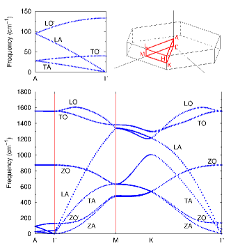
Figure 1: (Color online) Graphite phonon dispersion calculated with the optB88-vdW functional starting from the optimized equilibrium structure.Not On top left and right an enlargement of the low-frequency $\Gamma$-A region and the Brillouin zone with the high-symmetry points are shown, respectively.

The calculated phonon dispersions are in good agreement with experiments.Maultzsch et al. (2004); Oshima et al. (1988); Yanagisawa et al. (2005); Siebentritt et al. (1997); Nicklow et al. (1972) This is evident from Table 2, which lists phonon frequencies at the high-symmetry points $A$, $\Gamma$, $M$, and $K$, see also Ref. Mounet and Marzari, 2005. The labels $L$, $T$ and $Z$ denote longitudinal, in-plane transversal and out-of-plane transversal polarization respectively. A primed O (O^′) labels an optical mode where within the layers the atoms oscillate in phase whereas the two layers in the unit cell oscillate in anti-phase. An unprimed optical mode is a mode where atoms inside the same layer move in opposite directions.

Table 2: Phonon frequencies of graphite computed with the optB88 functional at the high-symmetry points $A$, $\Gamma$, $M$, and $K$ in cm^-1, compared to experimental results Maultzsch et al. (2004); Oshima et al. (1988); Yanagisawa et al. (2005); Siebentritt et al. (1997); Nicklow et al. (1972); Tuinstra and Koenig (1970).

	optB88-vdW	Experiment
$A\rm_{TA/TO^{\prime}}$	28	35
$A\rm_{LA/LO^{\prime}}$	95	89
$A\rm_{LO}$	873
$A\rm_{TO}$	1555
$\Gamma\rm_{LO^{\prime}}$	40	49
$\Gamma\rm_{ZO^{\prime}}$	139	95, 126
$\Gamma\rm_{ZO}$	870	861
$\Gamma\rm_{LO/TO}$	1553, 1558	1575, 1590
$M\rm_{ZA}$	471	471, 465, 451
$M\rm_{TA}$	628	630
$M\rm_{ZO}$	632	670
$M\rm_{LA}$	1335	1290
$M\rm_{LO}$	1340	1321
$M\rm_{TO}$	1383	1388, 1389
$K\rm_{ZA}$	534	482, 517, 530
$K\rm_{ZO}$	540	588, 627
$K\rm_{TA}$	1005
$K\rm_{LA/LO}$	1216	1184, 1202
$K\rm_{TO}$	1302	1313, 1291

Note in particular that the low frequency modes (below $\sim 150$ cm^-1) between $\Gamma$ and $A$, which are particularly sensitive to the interlayer coupling, are well reproduced. This is not the case if one uses GGA (PBE-PBE) without vdW contributions, where the frequencies of the low-energy modes in particular are strongly underestimated.Mounet and Marzari (2005) Forcing the experimental $c/a$ ratio upon the graphite structure largely repairs this deficit and yields sensible vibration frequencies.Mounet and Marzari (2005) However, such a procedure requires input of experimental data.

Elastic properties are a second good test for the quality of the potential energy surface predicted by the first-principles calculations. Table 3 shows the elastic properties of graphite calculated with the optB88-vdW functional. To obtain the elastic constants we perform ground state total-energy calculations over a broad range of lattice parameters: $2.20\leq a\leq 2.68$ Å and $4.00\leq c\leq 11.00$ Å. The calculated results are then fitted to a two-dimensional sixth order polynomial. The stiffness coefficients $C_{11}+C_{22}$, $C_{33}$ and $C_{13}$ are obtained as second derivatives of the energy with respect to $a$, $c$ and both $a$ and $c$, respectively. The bulk modulus $B_{0}$ and the tetragonal shear modulus $C^{t}$ are obtained from the stiffness coefficients. The procedure is similar to that of Ref. Mounet and Marzari, 2005.

Table 3: Elastic properties of graphite computed with the optB88 functional compared with the results from LDA, GGA, vdW-DF (revPBE) and RPA calculations, as well as with experiments. All data are in GPa

	$C_{11}+C_{22}$	$C_{33}$	$C_{13}$	$B_{0}$	$C^{t}$
this work	1200	35	$-6.7$	33	216
GGA	1230	45	$-4.6$	41.2	223
optB88-vdW		38
revPBE-vdW		27
ACFDT-RPA		36
Exp. (300 K)	1240$\pm$40	36.5$\pm$1	15$\pm$5	35.8	208.8

Table 3 compares our calculated elastic constants to experimental results,ela (2001); Blakslee et al. (1970) as well as to results obtained from GGA, vdW-DF (revPBE-vdW) and RPA calculations.Mounet and Marzari (2005); Ziambaras et al. (2007); Lebègue et al. (2010) The elastic constant $C_{33}\propto\partial^{2}E/\partial c^{2}$ probes the interlayer interaction and is sensitive to the vdW interactions. Our value is in very good agreement with experiment and with the result obtained from a ACFDT-RPA calculation.ela (2001); Lebègue et al. (2010) It is a definite improvement over GGA [PBE-PBE] results (even when imposing the experimental $c/a$ ratio).Mounet and Marzari (2005) A similar improvement is observed for the bulk modulus $B_{0}$.

Note that the revPBE-vdW functional gives a $C_{33}$ that is somewhat too small, compared to experiment. Apparently, the revPBE-vdW functional gives an energy curve for the binding between the graphene layers that is somewhat too shallow, which is consistent with the fact that the revPBE-vdW equilibrium distance is somewhat too large, see Table 1. In this respect the optB88-vdW functional performs better, although it gives an interlayer binding energy that is somewhat too large. In fact, all elastic constants obtained with optB88-vdW are in good agreement with experiment, except for $C_{13}$.

III.2 Li intercalation

The intercalation of Li in graphite leads to compounds Li_xC₆ with $0\leq x\leq 1$ with different structures as a function of the Li content $x$. We consider a large number of possible Li_nC_m ($x=6n/m$) structures and compositions, see Sec. III.2.2, where we use the optB88-vdW functional in all calculations, unless explicitly mentioned otherwise. In all cases the cell parameters, as well as the atomic positions, are optimized. The intercalation energy $E_{\rm int}$ per Li atom is defined as

$$E_{\rm int}({\rm Li}_{n}{\rm C}_{m})=\frac{1}{n}E({\rm Li}_{n}{\rm C}_{m})-E({\rm Li_{\rm metal}})-\frac{m}{4n}E_{\rm Gr},$$ (2)

where $E({\rm Li}_{n}{\rm C}_{m})$ is the total energy per formula unit of the Li_nC_m (Li_6n/mC₆) phase, $E({\rm Li_{\rm metal}})$ is the total energy per atom of bcc bulk Li, and $E_{\rm Gr}$ is the total energy of one graphite unit cell (containing four carbon atoms). Alternatively the intercalation energy can be referred to the free Li atom by subtracting the cohesive energy of the Li metal (1.578 eV/Li atom with optB88-vdW). Note that a negative value for $E_{\rm int}$ means that the intercalated compound is stable with respect to graphite and Li metal.

III.2.1 $\mathrm{LiC}_{6}$ and $\mathrm{Li}_{0.5}\mathrm{C}_{6}$

We start with the fully loaded stage 1 compound LiC₆ and stage 2 compound Li_0.5C₆ (LiC₁₂). The stage 1 compound has -A-Li-A-Li- stacking with an optimized graphene interlayer distance of 3.64 Å, which is close to the experimental value of 3.70 Å.Takami et al. (1995) For the fully lithiated stage 2 compound we consider both -A-Li-A-A-Li-A- and -A-Li-A-B-Li-B- stacking, and find that, in agreement with experiment,Billaud et al. (1996) the former is favored over the latter. The calculated difference in intercalation energy is 32 meV/Li. The optimized average distance between the graphene layers in LiC₁₂ is 3.49 Å, and the distance between the empty graphene layers is 3.27 Å. These numbers are in good agreement with the experimental values of 3.51 Å and 3.27 Å, respectively.Billaud et al. (1996); Takami et al. (1995) Evidently the optB88-vdW functional accurately reproduces the structures of LiC₆ and Li_0.5C₆.

Figure 2: (Color online) From top to bottom: phonon density of states (PhDOS) of stage 1 compound LiC₆, stage 2 compound LiC₁₂, pure graphite, and bcc Li metal. The red line gives the total PhDOS, and the blue and black lines give the contributions of, respectively, the carbon and lithium atoms to the normal modes.

The calculated intercalation energies for the stage 1 and stage 2 compounds LiC₆ and LiC₁₂ are $-0.217$ and $-0.273$ eV/Li, respectively, indicating the relative stability of the stage 2 compound. The intercalation free energies of the stage 1 and 2 compounds, extracted from electrochemical measurements at 300 K, are $-0.156$ and $-0.227$ eV/Li, respectively.Ohzuku et al. (1993) The intercalation enthalpies of LiC₆ and LiC₁₂ obtained from calorimetric measurements at 455 K with respect to liquid Li, are $-0.144$ and $-0.257$ eV/Li, respectively.Avdeev et al. (1996) Converting to solid Li as a reference state,fus ; Imai and Watanabe (2007) these enthalpies become $-0.113$ and $-0.226$ eV/Li. Even without including vibrational and finite temperature effects (to be discussed below), the calculations give intercalation energies that are consistently more negative than those obtained experimentally.not (a) Part of this might be due to an error we make in describing the Li metal. For instance, the atomization energy of the Li metal comes out 0.1 eV too small with the optB88-vdW functional.Klimeš et al. (2011)

So far we have not considered the vibrational contributions. The calculated phonon densities of states (PhDOS) of LiC₆ and LiC₁₂ are given in Fig. 2. They can be compared to the PhDOSs of pure graphite and bulk Li metal. Whereas the phonon spectrum of graphite includes frequencies of up to 50 THz, see also Fig. 1 and Table 2, the phonon frequencies in bulk Li are all below 10 THz. The PhDOSs of LiC₆ and LiC₁₂ reflect this division into two frequency regimes. The low frequency modes definitely have a mixed carbon lithium character, whereas in the high frequency modes only carbon atoms participate. Comparing to the pure graphite and bulk Li spectra there are significant changes, however.

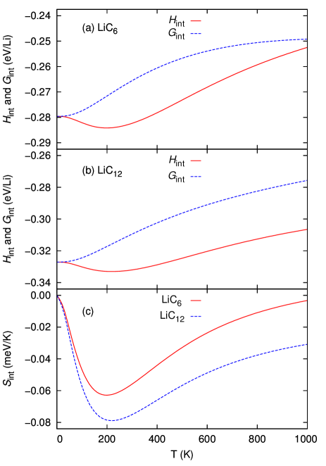
Figure 3: (Color online) The intercalation enthalpy $H_{\mathrm{int}}$, see Eq. (2), entropy $S_{\mathrm{int}}$, and free energy $G_{\mathrm{int}}=H_{\mathrm{int}}-TS_{\mathrm{int}}$, of the stage 1 compound LiC₆ and the stage 2 compound LiC₁₂, including the phonon contributions.

The PhDOS at high frequencies of lithiated graphite is clearly shifted to lower frequencies, as compared to the PhDOS of pure graphite. Upon Li intercalation the in-plane C-C bond length becomes larger and the bonds become weaker, as Li atoms donate electrons to the $\pi^{*}$ anti-bonding states of graphite. This leads to lower vibrational C-C stretch frequencies, which is noticeable in the high frequency range. There are also changes in the low frequency range, where vibrational modes concerning the motion of Li atoms are found. A double peak structure in the PhDOS between 6 and 14 THz can be identified, and assigned to modes where the Li atoms vibrate in the $ab$-plane, or along the $c$-axis, with the latter vibrations having the highest frequency. On average, the vibrational frequencies of intercalated Li atoms clearly are larger than those in bulk Li, indicating that intercalation confines the motion of the Li atoms.

Zero-point vibrational energies (ZPEs) are dominated by high frequency modes, which in this case are the stretch modes of the carbon lattice. As the frequencies of such modes are lower in intercalated graphite than in pure graphite, it means that the ZPE in intercalated graphite is lower. Hence the ZPE gives a negative contribution to the intercalation energy. Indeed, including zero-point vibrational energies (ZPEs) changes the intercalation energies by $-0.04$ and $-0.05$ eV/Li for LiC₆ and LiC₁₂, respectively.

The temperature dependence of the intercalation free energy of LiC₆ and LiC₁₂ is also determined by the phonons, as there is no contribution from configurational entropy in these fully lithiated compounds. The vibrational energy and entropy contributions to the intercalation enthalpy, entropy, and free energy can be calculated using standard harmonic oscillator expressions.van Setten et al. (2008); Hazrati et al. (2011) The thermodynamic quantities are shown in Fig. 3. The intercalation enthalpy hardly changes over the temperature range 0-400 K. This makes sense as the vibrational contributions are dominated by the high frequency modes, and the occupancy of these modes is not very sensitive to the temperature in this range. Note that the intercalation entropy is negative, and goes through a distinct minimum around 200 K. The entropy is dominated by the low-frequency modes. The stiffening of the Li vibrational modes in intercalated graphite (with respect to Li metal) reduces the entropy, resulting in a negative intercalation entropy. This effect has been observed experimentally.Reynier et al. (2004, 2003) Adding enthalpy and entropy contributions yields an intercalation free energy that is monotonically increasing with temperature.

The ZPE contribution to the intercalation energies of Li_xC₆ is almost constant for $x\gtrsim 0.375$, and one can expect it to be smaller for $x<0.375$. In the following we compare relative intercalation energies for different $x$. The ZPE contribution is then relatively unimportant, hence we do not consider it from here on.

III.2.2 $\mathrm{Li}_{x}\mathrm{C}_{6}$; $x<0.5$

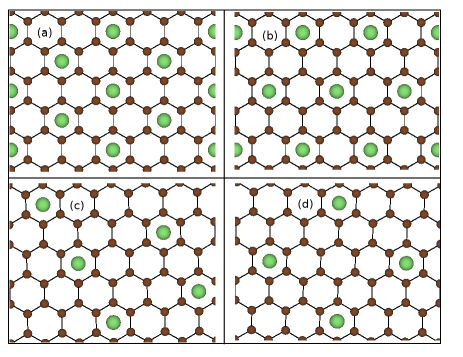
Figure 4: (Color online) Examples of stage 2 compounds with different in-plane Li ordering: (a) LiC₁₂ with $\sqrt{3}\times\sqrt{3}$ Li ordering, (b) LiC₁₆ with $2\times 2$ Li ordering, (c) LiC₂₄ with $\sqrt{7}\times 2$ Li ordering, and (d) LiC₃₂ with $\sqrt{7}\times\sqrt{7}$ Li ordering. For simplicity, only AA stackings are shown.

Table 4: Optimized structures of selected stage 2 compounds LiC_m; $m$ $\geq$ 12 (Li_xC₆) with $n\times m$ in-plane unit cells, stage 1 compound LiC₆, and graphite C₆; $d_{\rm av}$ is the average interlayer distance, in Å; $E_{\rm int}$ is the intercalation energy in eV/Li (without ZPEs).

	$x$	stack	$n\times m$	$d_{\rm av}$	$E_{\rm int}$
C6	0	AB	1$\times$1	3.36	0
LiC48	1/8	AABB	$\sqrt{7}\times 4$	3.48	$-0.256$
LiC40	3/20	AABB	$\sqrt{7}\times\sqrt{13}$	3.49	$-0.274$
LiC36	1/6	AABB	$\sqrt{7}\times 3$	3.50	$-0.275$
LiC32	3/16	AABB	$\sqrt{7}\times\sqrt{7}$	3.48	$-0.282$
LiC24	1/4	AABB	$\sqrt{7}\times 2$	3.51	$-0.270$
LiC20	3/10	AABB	$\sqrt{3}\times\sqrt{7}$	3.51	$-0.263$
LiC20	3/10	AA	$\sqrt{3}\times\sqrt{7}$	3.54	$-0.239$
LiC16	3/8	AABB	$2\times 2$	3.53	$-0.263$
LiC16	3/8	AA	$2\times 2$	3.53	$-0.261$
LiC16	3/8	AA	$\sqrt{3}\times 2$	3.53	$-0.257$
LiC12	1/2	AA	$\sqrt{3}\times\sqrt{3}$	3.49	$-0.273$
LiC6	1	AA	$\sqrt{3}\times\sqrt{3}$	3.65	$-0.217$

Whereas the structures of the fully lithiated stage 1 and stage 2 compounds are experimentally well established, less is known about the possible structures of Li_xC₆; $x<0.5$. As a first step, we have constructed a number of dilute stage-2 structures with compositions Li_xC₆, $1/8\leq x\leq 1/2$, and $n\times m$ in-plane Li lattices, $\sqrt{3}\leq n,m\leq 4$. Examples of such structures are shown in Fig. 4. The calculated optimized structural properties and intercalation energies of selected structures are listed in Table 4. As all these energies are negative, it follows that intercalation is favorable at any Li concentration.

Li intercalation in graphite becomes more favorable upon increasing the concentration up to $x=3/16$. In the concentration range $3/16<x\leq 1$ Li intercalation becomes slightly less favorable. The average interlayer spacing $d_{\rm av}$ tends to increase with the Li concentration $x$. Exceptions are $x=3/16$ and $x=1/2$, which coincide with minima in $E_{\rm int}(x)$. For these compositions that yield particular stable structures, $d_{\rm av}$ is smaller than that of adjacent compositions. Note that the most stable stacking of the graphene planes is AA-type for $x>3/8$, i.e., -A-Li-A-A-Li-A-. The stacking changes to AABB-type (-A-Li-A-B-Li-B-) for lower Li concentrations, however. Whereas the intercalation energies of AA and AABB stackings are within 2 meV/Li of one another for $x=3/8$, the difference increases to 150 meV/Li in favor of the AABB stacking for $x=1/8$.

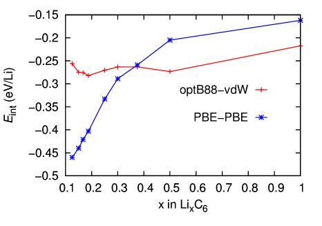
Figure 5: (Color online) The intercalation energy $H_{\mathrm{int}}$, see Eq. (2) of the dilute stage 2 compounds Li_xC₆, calculated with the optB88-vdW (red) and PBE-PBE (blue) functionals.

To stress the importance of vdW interaction for the energetics of intercalation, Fig. 5 shows the Li intercalation energies calculated with the optB88-vdW and the PBE-PBE functionals (using optB88-vdW geometries). As the latter functional lacks vdW interactions that give the interlayer bonding in graphite, intercalation of any amount of Li lowers the energy, as Li binds to the graphene planes. The bonding is partially ionic as Li donates electrons to the carbon lattice.Er et al. (2009) The Coulomb repulsion between Li atoms/ions can be minimized in a diluted intercalation structure, which means that in absence of vdW interactions the intercalation energy monotonically increases with Li concentration. However, vdW interactions between the graphene planes oppose this trend. Intercalation disrupts the stacking of graphene planes, so vdW interactions prefer to cluster Li atoms such as to minimize the spatial extend of these disruptions.

Omitting vdW interactions thus leads to an net overestimation of the effect of Li-graphene attractions in Li_xC₆ compounds with small $x$ and a net overestimation of the Li-Li repulsions for large $x$. Hence, the intercalation energy is too small (i.e., too negative) for small $x$, and too large for large $x$. The PBE-PBE intercalation energy is a monotonically increasing function of $x$, instead of having minima at a specific $x$. It means that PBE-PBE yields Li_xC₆ compounds where the Li concentration $x$ is a simple monotonic function of the Li chemical potential, like in a simple lattice gas. This is clearly at variance with experiment, where phases with specific compositions are found to be thermodynamically stable.Dahn (1991); Ohzuku et al. (1993); Senyshyn et al. (2013); Billaud et al. (1996); Filhol et al. (2008)

The balance between the graphene-graphene vdW bonding and the Li-graphene bonding gives the optB88-vdW curve shown in Fig. 5. The curve has two shallow minima at concentrations $x=3/16$ and $x=1/2$, respectively. The latter corresponds to the fully loaded stage 2 compound, where the Li atoms order in plane in a regular $\sqrt{3}\times\sqrt{3}$ lattice, as shown in Fig. 4. The $x=3/16$ structure corresponds to a dilute stage 2 compound, where the Li atoms order in plane in a regular $\sqrt{7}\times\sqrt{7}$ lattice, see Fig. 4. One should note however that several other dilute stage 2 structures with compositions $x\leq 0.5$ have an intercalation energy within 20 meV of the two structures of Fig. 4. We will come back to this point later.

Such dilute stage 2 structures, where partially loaded layers alternate with empty layers, are in fact more stable than stage 3-5 structures of the same composition Li_xC₆, where fully loaded layers are separated by more than one empty layer. The calculated optimized structural properties and intercalation energies of selected stage 3-5 structures are listed in Table 5. It means that, according to the calculations, it is not likely that stage 3-5 structures are formed during loading of graphite with Li.

Table 5: As Table 4 but for stage N compounds LiC_m with $\sqrt{3}\times\sqrt{3}$ in-plane unit cells.

	$x$	stack	N	$d_{\rm av}$	$E_{\rm int}$
C6	0	AB	-	3.36	0
LiC30	1/5	AABAB	5	3.44	$-0.219$
LiC24	1/4	AABABBAB	4	3.44	$-0.243$
LiC18	1/3	AAB	3	3.46	$-0.242$
LiC12	1/2	AA	2	3.49	$-0.273$
LiC6	1	AA	1	3.65	$-0.217$

III.2.3 Stable phases

Intercalation energies for a large number of structures and different compositions are given in Fig. 6(a). In agreement with the results shown in the previous subsection the two stage 2 Li_xC₆ structures with $x=3/16$ and $x=1/2$ give the optimal intercalation, corresponding to in-plane $\sqrt{7}\times\sqrt{7}$ and $\sqrt{3}\times\sqrt{3}$ orderings of Li atoms, respectively. Several dilute stage 2 structures with other compositions and slightly different in-plane orderings have slightly less favorable intercalation energies, but very different stage 2, or stage 1 and 3-5 structures have unfavorable intercalation energies.

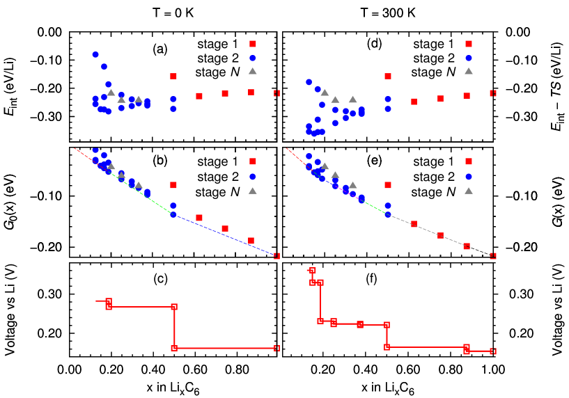
Figure 6: (Color online) (a) Intercalation energy (eV/Li) versus concentration $x$ in Li_xC₆ structures (b) Zero temperature (free) energy $G_{0}(x)$ (eV) of Li_xC₆ structures versus Li concentration $x$; (c) Calculated zero temperature voltage profile of Li_xC₆ structures versus Li concentration $x$. (d) Intercalation free energy (eV/Li) versus concentration $x$ in Li_xC₆ structures at room temperature ($T=300$ K) (e) Room temperature (free) energy $G(x)$ (eV) of Li_xC₆ structures versus Li concentration $x$; (f) Calculated room temperature voltage profile of Li_xC₆ structures versus Li concentration $x$.

A structure Li_xC₆ is stable with respect to decomposition into Li${}_{x_{1}}$C₆ and Li${}_{x_{2}}$C₆, $x_{1}<x<x_{2}$, if its Gibbs free energy $G(x)$ is lower than that of the possible decomposition mixture, $[(x_{2}-x)G(x_{1})+(x-x_{1})G(x_{2})]/(x_{2}-x_{1})$. First we will consider zero temperature, where for solid states Gibbs free energies can be approximated by ground-state total energies,Aydinol et al. (1997)

$$G_{0}(x)\approx xE_{\mathrm{int}}(\mathrm{Li}_{n}\mathrm{C}_{m}),\;x=6n/m,$$ (3)

where we use graphite and Li metal as reference phases. The values of $G_{0}$ are given in Fig. 6(b) for the different structures and compositions $x$. Constructing a convex curve from straight line segments between the data points with $x$ that are lowest in energy, only the points on that curve represent stable phases. The segments represent the free energies of decomposition mixtures. From our calculations the only stable phases at $T=0$ are then the stage 2 compounds LiC₃₂ and LiC₁₂, and the stage 1 compound LiC₆, corresponding to $x=3/16$, 1/2 and 1, respectively.

Note that after starting the intercalation, first the phase appears with the lowest intercalation energy $E_{\mathrm{int}}$, i.e., LiC₃₂ ($x=3/16$). The following sequence of phases is then expected upon increasing the Li content. For $0<x<3/16$, graphite and the stage 2 compound LiC₃₂ coexist (red line in Fig. 6(b)), followed by a coexistence of the stage 2 compounds LiC₃₂ and LiC₁₂ for $3/16<x<1/2$ (green line), and finally a coexistence of the stage 2 compound LiC₁₂ and the stage 1 compound LiC₆ for $1/2<x<1$ (blue line). Experimentally the stability and structures of the LiC₁₂ and LiC₆ compounds are well established.Dahn (1991); Ohzuku et al. (1993); Senyshyn et al. (2013); Billaud et al. (1996); Filhol et al. (2008) Also quite consistently a stable phase with a composition around $x\approx 0.2$ is observed, which we attribute to the $\sqrt{7}\times\sqrt{7}$ dilute stage 2 structure. The experimental phase diagram between compositions $x\approx 0.2$ and 0.5 appears to be quite complicated. We attribute this to the effects of disorder entropy in the dilute stage 2 structures, to be discussed in the next subsection.

Experimentally the phase diagram of Li-graphite is often characterized by measuring the potential difference between a Li_xC₆ electrode and a Li metal electrode,Dahn (1991); Ohzuku et al. (1993)

$$V(x)=\frac{1}{e}\left[\mu_{\mathrm{metal}}-\mu(x)\right],$$ (4)

with $\mu_{\mathrm{metal}}$ the chemical potential of Li metal. The chemical potential of Li in Li_xC₆ $\mu(x)=\partial G(x)/\partial x$ is the derivative of the curve in Fig. 6(b). Because of the convex shape of this curve, $V$ is a monotonically decreasing function of $x$. In particular, if at any concentration $x$ two stable phases $x_{1}<x_{2}$ are in equilibrium, then the chemical potential is constant in this concentration range, and is given by the slope of the corresponding straight line segments in Fig. 6(b)

$$\mu(x)=\frac{G(x_{2})-G(x_{1})}{x_{2}-x_{1}};\;x_{1}\leq x<x_{2},$$ (5)

The potential $V(x)$ as a function of concentration is then a staircase, where each plateau characterizes a mixture of the stable compositions $x_{1}$ and $x_{2}$. The calculated potential for the Li-graphite system at $T=0$ is plotted in Fig. 6(c). Note that the first plateau after starting the intercalation should correspond to minus the intercalation energy $-E_{\mathrm{int}}$ of the first stable phase, which is LiC₃₂ ($x=3/16$), cf. Eq. (3)-(5). The calculated sequence of voltage plateaus then follows the sequence of mixtures of stable phases discussed above.

Compared to the voltages measured in experiment,Dahn (1991); Ohzuku et al. (1993); Reynier et al. (2004); Senyshyn et al. (2013); Billaud et al. (1996); Filhol et al. (2008) the calculated voltages are somewhat too high, e.g., by $\sim 50$ mV at $x=1$. The difference $\Delta V\approx-120$ mV between the $x<3/16$ and the $x>1/2$ plateaus, however, agrees quite well with experiment, suggesting that the calculated results include a constant offset. Again, part of this might be due to an error made in the description of Li metal. The shape of the voltage curve for $x<0.5$ is quite different from experiment. We attribute this to the effects of finite temperature, as will be discussed in the next subsection.

III.2.4 Finite temperature

As already mentioned, the configurational entropy is zero for the fully loaded stage 1 (LiC₆) and stage 2 (Li_0.5C₆) structures. The configurational entropy contribution to the intercalation free energy could be important, however, for the partially loaded stage 1 and stage 2 compounds in Table 4 and Figure 6(a-c). In this section we assess its effect. We ignore vibrational contributions to energy and entropy as they are only weakly dependent on composition.

To account for the configurational entropy $S^{\rm config}$, we follow the Bethe-Peierls method of Ref. Filhol et al., 2008 and treat the intermediate Li_xC₆ compositions as alloys of occupied and unoccupied Li lattice sites. Positions above the centers of C₆ hexagons count as possible lattice sites for Li atoms, as in the structures of Fig. 4, for example. An effective short range repulsion between Li atoms is introduced by excluding configurations where two Li atoms occupy two adjacent, i.e., edge sharing, hexagons, because that is energetically highly unfavorable.not (b) No longer range interactions between Li atoms are assumed, which means that we probably slightly overestimate the configurational entropy contribution to the free energy. The Bethe-Peierls model provides an exact statistical treatment of Li atoms occupying 7 sites in a hexagonal lattice (the central site and its first ring of neighbors). A mean field treatment accounts for the interactions with the rest of the lattice.

Subtracting $TS^{\rm config}$ from $E_{\rm int}$ and $xTS^{\rm config}$ from $G_{0}$, Eq. (3), we obtain the plots shown in Fig. 6(d-f), calculated for room temperature ($T=300$ K). Comparing Figs. 6(a) and (d) one observes that the configurational entropy contribution substantially lowers the intercalation (free) energy for some compositions. This also has a marked effect on the Gibbs free energies, shown in Fig. 6(e), where several intermediate compositions besides the $T=0$ structures for $x=3/16,1/2$ and $1$, are stabilized at $T=300$ K. Constructing the convex curve connecting the free energy minima we find stable compositions at $x=3/20,3/16,1/4,3/8,1/2,21/24$ and 1.

The calculated potential $V(x)$ at T = 300 K is plotted in Fig. 6(f). Comparing to the situation at $T=0$, Fig. 6(c), we observe that the steps at $x=3/16$ and $x=1/2$ remain prominent. The difference between the plateaus at $x<3/16$ and $x>1/2$ increases somewhat, from $\Delta V\approx-120$ mV ($T=0$) to $-160$ mV ($T=300$ K). The main difference lies in the shape of the curve for intermediate compositions $3/16<x<1/2$, where entropy effects at finite temperature lead to a decrease of the potential step at $x=1/2$ and a concomitant increase of the step at $x=3/16$. Intermediate compositions are also stabilized, but only lead to small potential steps, indicating that the Gibbs free energy $G(x)$ of the (disordered) dilute stage 2 compound is nearly linear in $x$ in this range. The potential rises again at $x\leq 3/20$, but for smaller $x$ the calculations become increasingly more difficult.

The voltage curve shown in Fig. 6(f) is in line with what is found in experiments, where a small potential step is typically observed at $x=0.5$, a larger one at or close to $x=0.2$, and further increases of the potential for smaller $x$.Dahn (1991); Ohzuku et al. (1993); Reynier et al. (2004); Senyshyn et al. (2013); Billaud et al. (1996); Filhol et al. (2008) Evidently including entropy effects leads to a decent description of the voltage curve. It also implies that the curve for $x\leq 0.5$ can be interpreted on the basis of stage 2 compounds only, and that there is no need to invoke stage $N>2$ compounds.

Entropy effects were also studied in Ref. Filhol et al., 2008, for stage 1 compounds with compositions in the range $0.5\leq x\leq 1$, where vdW contributions are likely to be less important. That study employed LDA and GGA functionals without vdW corrections, and found a stabilization at 300 K of the two compositions $x\approx 0.55$ and $x\approx 0.88$. With the vdW functional we find the composition $x=0.875$ stabilized at $T=300$ K, but we have not considered structures with compositions near $0.55$. In view of the different functionals used, we consider this good agreement. The calculated potential step at $x=0.875$ is small, see Fig. 6(f), and it hardly changes the potential curve, as compared to the zero temperature curve, see Fig. 6(c).

IV Summary and conclusions

Li/graphite is the archetypical intercalation system. As a material it is of utmost importance for applications in rechargeable Li-ion batteries. It shows a remarkable palette of structures and phases as a function of the Li concentration Li_xC₆, $0<x\leq 1$. Accurately modeling layered intercalation compounds from first principles has hitherto been very difficult, as their structure is often determined by a fine balance between van der Waals (vdW) interactions and chemical or Madelung interactions, and standard first-principles techniques lack a good description of vdW interactions.

Using recently proposed vdW density functionals we study the structures and the energetics of bulk graphite and Li-graphite intercalation compounds. Different versions of vdW functionals are benchmarked on bulk graphite, where they give a good description of the bonding and the structural properties. Selecting the functional that yields the most accurate structure (optB88-vdW) one also finds an accurate description of the graphite phonon band structure and the elastic constants from first principles.

Intercalation of Li in graphite leads to stable systems with calculated intercalation energies of $-0.2$ to $-0.3$ eV/Li atom (referred to bulk graphite and Li metal). The calculations give negative intercalation entropies of $-0.06$ to $-0.08$ meV/K/Li atom at room temperature resulting from the phonon contributions, demonstrating that the motion of Li atoms in the intercalated compound is more constrained than in the bulk Li metal.

The fully loaded stage 1 and stage 2 compounds LiC₆ and Li_1/2C₆ are thermodynamically stable, corresponding to two-dimensional $\sqrt{3}\times\sqrt{3}$ lattices of Li atoms intercalated between each pair of graphene planes, or every other pair, respectively. Stage $N>2$ compounds, consisting of a $\sqrt{3}\times\sqrt{3}$ lattice of Li atoms intercalated between two graphene planes alternating with $N-1$ empty layers, are predicted to be unstable. Instead, upon decreasing the Li concentration it is more advantageous to decrease the packing of Li atoms in the stage 2 compound. The compound Li_3/16C₆ is particularly stable; it corresponds to a $\sqrt{7}\times\sqrt{7}$ in-plane packing of Li atoms.

Apart from a short-range repulsion the effective in-plane interaction between Li atoms in stage 2 compounds is relatively weak. At elevated temperatures dilute stage 2 compounds Li_xC₆, $x<0.5$ are therefore easily disordered. Even at room temperature the relative stability of the Li_3/16C₆ and Li_1/2C₆ structures can still be recognized, however. The voltage profile extracted from the calculations is in reasonable agreement with experiments, which demonstrates the improvements of first-principles techniques in calculating the properties of intercalation compounds.

References

- Dresselhaus and Dresselhaus (2002) M. S. Dresselhaus and G. Dresselhaus, Adv. Phys. 51, 1 (2002).
- Pan et al. (2011) Z.-H. Pan, J. Camacho, M. H. Upton, A. V. Fedorov, C. A. Howard, M. Ellerby, and T. Valla, Phys. Rev. Lett. 106, 187002 (2011).
- Csanyi et al. (2005) G. Csanyi, P. B. Littlewood, A. H. Nevidomskyy, C. J. Pickard, and B. D. Simons, Nat. Phys. 1, 42 (2005).
- Petrović et al. (2013) M. Petrović, I. Šrut Rakić, S. Runte, C. Busse, J. T. Sadowski, P. Lazić, I. Pletikosić, Z.-H. Pan, M. Milun, P. Pervan, et al., Nat. Commun. 4, 2772 (2013).
- Bao et al. (2014) W. Bao, J. Wan, X. Han, X. Cai, H. Zhu, D. Kim, D. Ma, Y. Xu, J. N. Munday, H. D. Drew, et al., Nat. Commun. 5, 4224 (2014).
- Weller et al. (2005) T. E. Weller, M. Ellerby, S. S. Saxena, R. P. Smith, and N. T. Skipper, Nat. Phys. 1, 39 (2005).
- Cabaret et al. (2013) D. Cabaret, N. Emery, C. Bellin, C. Hérold, P. Lagrange, F. Wilhelm, A. Rogalev, and G. Loupias, Phys. Rev. B 87, 075108 (2013).
- Dahn et al. (1995) J. R. Dahn, T. Zheng, Y. Liu, and J. S. Xue, Science 270, 590 (1995).
- Winter et al. (1998) M. Winter, J. O. Besenhard, M. E. Spahr, and P. Novák, Adv. Mater. 10, 725 (1998).
- Endo et al. (2000) M. Endo, C. Kim, K. Nishimura, T. Fujino, and K. Miyashita, Carbon 38, 183 (2000).
- Kaskhedikar and Maier (2009) N. A. Kaskhedikar and J. Maier, Adv. Mater. 21, 2664 (2009).
- Dahn (1991) J. R. Dahn, Phys. Rev. B 44, 9170 (1991).
- Ohzuku et al. (1993) T. Ohzuku, Y. Iwakoshi, and K. Sawai, J. Electrochem. Soc. 140, 2490 (1993).
- Senyshyn et al. (2013) A. Senyshyn, O. Dolotko, M. J. Mühlbauer, K. Nikolowski, H. Fuess, and H. Ehrenberg, J. Electrochem. Soc. 160, A3198 (2013).
- Billaud et al. (1996) D. Billaud, F. Henry, M. Lelaurain, and P. Willmann, J. Phys. Chem Solids 57, 775 (1996).
- Reynier et al. (2004) Y. F. Reynier, R. Yazami, and B. Fultz, J. Electrochem. Soc. 151, A422 (2004).
- Chevallier et al. (2013) F. Chevallier, F. Poli, B. Montigny, and M. Letellier, Carbon 61, 140 (2013).
- Gross et al. (2008) A. F. Gross, J. J. Vajo, S. L. Van Atta, and G. L. Olson, J. Phys. Chem. C 112, 5651 (2008).
- Ngene et al. (2010) P. Ngene, R. van Zwienen, and P. E. de Jongh, Chem. Comm. 46, 8201 (2010).
- Liu et al. (2011) X. Liu, D. Peaslee, C. Z. Jost, T. F. Baumann, and E. H. Majzoub, Chem. Mater. 23, 1331 (2011).
- Hazrati et al. (2014) E. Hazrati, G. Brocks, and G. A. de Wijs, J. Phys. Chem. C 118, 5101 (2014).
- Filhol et al. (2008) J.-S. Filhol, C. Combelles, R. Yazami, and M.-L. Doublet, J. Phys. Chem. C 112, 3982 (2008).
- Langer et al. (2013) J. Langer, V. Epp, P. Heitjans, F. A. Mautner, and M. Wilkening, Phys. Rev. B 88, 094304 (2013).
- Bhattacharya and Van der Ven (2011) J. Bhattacharya and A. Van der Ven, Phys. Rev. B 83, 144302 (2011).
- Morgan and Madden (2012) B. J. Morgan and P. A. Madden, Phys. Rev. B 86, 035147 (2012).
- Persson et al. (2010) K. Persson, Y. Hinuma, Y. S. Meng, A. Van der Ven, and G. Ceder, Phys. Rev. B 82, 125416 (2010).
- Kohn and Sham (1965) W. Kohn and L. J. Sham, Phys. Rev. 140, A1133 (1965).
- Perdew et al. (1996) J. P. Perdew, K. Burke, and M. Ernzerhof, Phys. Rev. Lett. 77, 3865 (1996).
- Hohenberg and Kohn (1964) P. Hohenberg and W. Kohn, Phys. Rev. 136, B864 (1964).
- Kganyaga and Ngoepe (2003) K. R. Kganyaga and Ngoepe, Phys. Rev. B 68, 205111 (2003).
- Could et al. (2013) T. Could, S. Lebègue, and J. F. Dobson, J. Phys.: Condens. Matter 25, 445010 (2013).
- Grimme (2006) S. Grimme, J. Comput. Chem. 27, 1787 (2006).
- Er et al. (2009) S. Er, G. A. de Wijs, and G. Brocks, J. Phys. Chem. C 113, 8997 (2009).
- Lee and Persson (2012) E. Lee and K. A. Persson, Nano Lett. 12, 4624 (2012).
- Spanu et al. (2009) L. Spanu, S. Sorella, and G. Galli, Phys. Rev. Lett. 103, 196401 (2009).
- Lebègue et al. (2010) S. Lebègue, J. Harl, T. Gould, J. G. Ángyán, G. Kresse, and J. F. Dobson, Phys. Rev. Lett. 105, 196401 (2010).
- Rydberg et al. (2000) H. Rydberg, B. I. Lundqvist, D. C. Langreth, and M. Dion, Phys. Rev. B 62, 6997 (2000).
- Rydberg et al. (2003) H. Rydberg, M. Dion, N. Jacobson, E. Schröder, P. Hyldgaard, S. I. Simak, D. C. Langreth, and B. I. Lundqvist, Phys. Rev. Lett. 91, 126402 (2003).
- Dion et al. (2004) M. Dion, H. Rydberg, E. Schröder, D. C. Langreth, and B. I. Lundqvist, Phys. Rev. Lett. 92, 246401 (2004).
- Thonhauser et al. (2007) T. Thonhauser, V. R. Cooper, S. Li, A. Puzder, P. Hyldgaard, and D. C. Langreth, Phys. Rev. B 76, 125112 (2007).
- Blöchl (1994) P. E. Blöchl, Phys. Rev. B 50, 17953 (1994).
- Kresse and Joubert (1999) G. Kresse and D. Joubert, Phys. Rev. B 59, 1758 (1999).
- Kresse and Furthmüller (1996a) G. Kresse and J. Furthmüller, Phys. Rev. B 54, 11169 (1996a).
- Kresse and Furthmüller (1996b) G. Kresse and J. Furthmüller, Comput. Mater. Sci. 6, 15 (1996b).
- Klimeš et al. (2010) J. Klimeš, D. R. Bowler, and A. Michaelides, J. Phys.: Condens. Matter 22, 022201 (2010).
- Klimeš et al. (2011) J. Klimeš, D. R. Bowler, and A. Michaelides, Phys. Rev. B 83, 195131 (2011).
- Román-Pérez and Soler (2009) G. Román-Pérez and J. M. Soler, Phys. Rev. Lett. 103, 096102 (2009).
- Zhang and Yang (1998) Y. Zhang and W. Yang, Phys. Rev. Lett. 80, 890 (1998).
- Lee et al. (2010) K. Lee, E. D. Murray, L. Kong, B. I. Lundqvist, and D. C. Langreth, Phys. Rev. B 82, 081101 (2010).
- Perdew and Wang (1986) J. P. Perdew and Y. Wang, Phys. Rev. B 33, 8800 (1986).
- (51) Both cell shape and positions were relaxed for a set of fixed volumes. The final equilibrium volume and the ground state energy were obtained by a fit to an equation of state.
- Kresse et al. (1995) G. Kresse, J. Furthmüller, and J. Hafner, Europhys. Lett. 32, 729 (1995).
- Methfessel and Paxton (1989) M. Methfessel and A. T. Paxton, Phys. Rev. B 40, 3616 (1989).
- Baskin and Meyer (1955) Y. Baskin and L. Meyer, Phys. Rev. 100, 544 (1955).
- Zacharia et al. (2004) R. Zacharia, H. Ulbricht, and T. Hertel, Phys. Rev. B 69, 155406 (2004).
- Hamada and Otani (2010) I. Hamada and M. Otani, Phys. Rev. B 82, 153412 (2010).
- Mapasha et al. (2012) R. E. Mapasha, A. M. Ukpong, and N. Chetty, Phys. Rev. B 85, 205402 (2012).
- Graziano et al. (2012) G. Graziano, J. Klimeš, F. Fernandez-Alonso, and A. Michaelides, J. Phys.: Condens. Matter 24, 424216 (2012).
- Bernal (1924) J. D. Bernal, Proc. R. Soc. Lond. A 106, 749 (1924).
- Charlier et al. (1994) J.-C. Charlier, X. Gonze, and J.-P. Michenaud, Europhys. Lett. 28, 403 (1994).
- Wang et al. (2014) Z. Wang, S. M. Selbach, and T. Grande, RSC Adv. 4, 4069 (2014).
- (62) Supercells were used: For -A the cell was doubled along . For -M, we used a cell, i.e. 4 times repeated along and along . The phonons for the line -K-M were obtained from an orthorhombic supercell with sides .
- Maultzsch et al. (2004) J. Maultzsch, S. Reich, C. Thomsen, H. Requardt, and P. Ordejón, Phys. Rev. Lett. 92, 075501 (2004).
- Oshima et al. (1988) C. Oshima, T. Aizawa, R. Souda, Y. Ishizawa, and Y. Sumiyoshi, Solid State Commun. 65, 1601 (1988).
- Yanagisawa et al. (2005) H. Yanagisawa, T. Tanaka, Y. Ishida, M. Matsue, E. Rokuta, S. Otani, and C. Oshima, Surf. Interface Anal. 37, 133 (2005).
- Siebentritt et al. (1997) S. Siebentritt, R. Pues, K.-H. Rieder, and A. M. Shikin, Phys. Rev. B 55, 7927 (1997).
- Nicklow et al. (1972) R. Nicklow, N. Wakabayashi, and H. G. Smith, Phys. Rev. B 5, 4951 (1972).
- Mounet and Marzari (2005) N. Mounet and N. Marzari, Phys. Rev. B 71, 205214 (2005).
- Tuinstra and Koenig (1970) F. Tuinstra and J. L. Koenig, J. Chem. Phys. 53, 1126 (1970).
- Ziambaras et al. (2007) E. Ziambaras, J. Kleis, E. Schröder, and P. Hyldgaard, Phys. Rev. B 76, 155425 (2007).
- ela (2001) Graphite and precursors, edited by P. Delhaes (Gordon and Breach, Australia, 2001).
- Blakslee et al. (1970) O. L. Blakslee, D. G. Proctor, E. J. Seldin, G. B. Spence, and T. Weng, J. Appl. Phys. 41, 3373 (1970).
- Takami et al. (1995) N. Takami, A. Satoh, M. Hara, and T. Ohsaki, J. Electrochem. Soc. 142, 371 (1995).
- Avdeev et al. (1996) V. V. Avdeev, A. P. Savchenkova, L. A. Monyakina, I. V. Nikol’skaya, and A. V. Khvostov, J. Phys. Chem Solids 57, 947 (1996).
- (75) The experimental enthalpy of fusion for Li at its melting point (453.7 K) is 3 kJ/mol.
- Imai and Watanabe (2007) Y. Imai and A. Watanabe, J. Alloy. Compd. 439, 258 (2007).
- not (a) Calculations using the LDA give intercalation energies for the stage 1 and stage 2 compounds LiC6 and LiC12 of and eV/Li, respectively, implying that LDA considerably overestimates the Li-graphite interaction.
- van Setten et al. (2008) M. J. van Setten, G. A. de Wijs, and G. Brocks, Phys. Rev. B 77, 165115 (2008).
- Hazrati et al. (2011) E. Hazrati, G. Brocks, B. Buurman, R. A. de Groot, and G. A. de Wijs, Phys. Chem. Chem. Phys. 13, 6043 (2011).
- Reynier et al. (2003) Y. Reynier, R. Yazami, and B. Fultz, J. Power Sources 119-121, 850 (2003).
- Aydinol et al. (1997) M. Aydinol, A. Kohan, and G. Ceder, J. Power Sources 68, 664 (1997).
- not (b) For the energy to move a Li from the next-nearest neighbour to the nearest neighbour position of another Li in the bilayer graphene we find 0.26 eV using optB88-vdW. See also Ref. Filhol et al., 2008.