Abstract

The baryon spectrum in the Sakai-Sugimoto model in the D4 background with smeared D0 charges is studied. We follow the instanton description of baryons by Hata et al.[Prog. Theor. Phys. 117, 1157]. The background corresponds to an excited state with nonzero glue condensate $\langle{\rm tr}(F_{\mu\nu}\tilde{F}^{\mu\nu})\rangle$ which is proportional to the D0 charge density. The baryon size shrinks when we turn on small D0 charge density. But for larger D0 charge density where massive modes in the gauge theory may also take effect, the size of baryons will grow. The difference between baryon masses will become smaller when D0 charge density increases. There may also be indications that the baryon will become unstable and cannot exist for sufficiently large D0 density.

1 Introduction

In recent years, with the running of the RHIC, there have been some discussions on the spontaneous parity violation in hot QCD. Some proposals were put forward that $P$- or $CP$- odd bubble may be created during the collisions [1, 2, 3]. A metastable state with nonzero QCD vacuum $\theta$ angle or $tr(F_{\mu\nu}\tilde{F}^{\mu\nu})$ could be produced in some space-time region in the hot and dense condition when deconfinement happens. According to the proposal, with the rapid expansion of the bubble, it cools down and the metastable state freezes inside the bubble[2, 4], returning to the confinement phase. Then a $P$- or $CP$-odd bubble forms and may soon decay into the true vacuum. Chiral magnetic effect was proposed as a test of this kind of phenomenon [5, 6]. See [7] for a review.

The state with nonzero $tr(F_{\mu\nu}\tilde{F}^{\mu\nu})$ may also play a role in the confinement mechanism. Many mechanisms were proposed as the possible cause of the confinement. See [8] for a review. Among these mechanisms, some classical or semiclassical gauge field configurations are important, such as some topologically nontrivial solutions—monopoles, instantons, and so on. In particular, there could be field configurations with constant field strength as solutions for the classical equation of motion or at the minimum of effective potential. Self-dual field strength is studied in [9, 10, 11, 12], and was proposed to be a mechanism for the confinement [13]. Some of these solutions come with nonzero $tr(F_{\mu\nu}\tilde{F}^{\mu\nu})$. There can also be domain solutions[9, 14, 15] that have different field strength pointing in diverse directions in different tiny space-time domains. By averaging over a larger length scale, some global symmetries, such as Poincaré symmetry, are recovered. In our paper, we are interested in the states with only $P$-parity non-conserved and the Poicaré invariance preserved, that is, states with nonzero $\langle tr(F_{\mu\nu}\tilde{F}^{\mu\nu})\rangle$ and vanishing $\langle F_{\mu\nu}\rangle$.

To study the effects of the states with nonzero $tr(F_{\mu\nu}\tilde{F}^{\mu\nu})$, one has to resort to some nonperturbative methods. String-gauge duality provides a powerful nonperturbative method to study this kind of phenomena. Adding $\langle tr(F_{\mu\nu}\tilde{F}^{\mu\nu})\rangle$ condensate to gauge theory was first studied in N=4 SUSY YM along these lines, and corresponds to adding smeared D(-1) charges into D3-brane configuration [16, 17]. Temperature and flavors can also be introduced into the Yang-Mills, and then quark condensates, meson spectra, baryon properties, etc., could be studied[17, 18, 19, 20, 21, 22, 23, 24, 25, 26, 27, 28].

Several other holographic constructions of the QCD-like theory are based on the D4 background initiated by Witten [29], which corresponds to the five-dimensional gauge theory compactified on a small circle to give a four-dimensional gauge theory. Among others, Sakai and Sugimoto proposed a promising model, which realizes the spontaneous chiral symmetry breaking by a geometric construction [30, 31]. In this model, flavors are realized by introducing $N_{f}$ D8-branes and $N_{f}$ anti-D8-branes which combine at the tip of the cigar geometry of the D4 soliton. This geometry is supposed to describe the spontaneously breaking of the $U_{L}(N_{f})\times U_{R}(N_{f})$ symmetry to $U_{V}(N_{f})$ in the four-dimensional theory, which is strengthened by the existence of the massless Goldstones in the spectrum. The low energy chiral Lagrangian for mesons can also be derived in this model. Similar to the D(-1)-D3 background, adding condensate $\langle tr(F_{\mu\nu}\tilde{F}^{\mu\nu})\rangle$ in the S-S model corresponds to adding smeared D0 charges into the D4 background. The gauge theory in this background is studied in [32, 33]. Putting Sakai-Sugimoto model (S-S model) into this background allows us to study the hadron phenomena in the nonzero $\langle tr(F_{\mu\nu}\tilde{F}^{\mu\nu})\rangle$ background. We have already studied the meson spectra and the interactions of the lowest-lying vector mesons and Goldstones in this background in [34] and found out that introducing $\langle tr(F_{\mu\nu}\tilde{F}^{\mu\nu})\rangle$ does not change the property of the spontaneous breaking of the $SU_{L}(N_{f})\times SU_{R}(N_{f})\to SU_{V}(N_{f})$. In the present paper, we will study the baryon mass spectrum in this background. As in [34], to keep the $\langle tr(F_{\mu\nu}\tilde{F}^{\mu\nu})\rangle$ dependence in the large $N_{c}$, we require it to be of ${\mathcal{O}}(N_{c})$ as in [16], $\tilde{\kappa}\sim\langle tr(F_{\mu\nu}\tilde{F}^{\mu\nu})\rangle/N_{c}$. Baryons can be turned on in the S-S model by introducing the baryonic D4-branes wrapping the sphere directions, which can be related to the Skyrmions in the low energy effective theory[30, 36]. This can be realized as the soliton solutions of the gauge fields on D8[37], and the nucleon interactions can also be modelled along these lines[38, 39, 40]. In [41], uniform distributed baryon system in the D0-D4 background is studied and the chiral condensate is discussed. We will follow the approach of [37], and study the $\tilde{\kappa}$ dependence of the baryon mass spectrum. We will see that there may be indications that the baryons may not be able to exist with strong $\tilde{\kappa}$ turned on with massive KK modes in the gauge theory included.

The structure of this paper is as follows: In section 2, we review the D0-D4 background and its relation to the gauge field theory following [34]. In section 3, we put the S-S model in this background and we study the soliton solution of the action at order of $\lambda^{0}$. In section 4 we use the collective coordinate quantization to obtain the mass spectrum of the baryons and their $\tilde{\kappa}$ dependence. Section 5 is the conclusion.

2 The D0-D4 background and the corresponding field theory

In this section, we review the D0-D4 background and its corresponding field theory following [32].

The solution of D4-branes with smeared D0 charges in type IIA supergravity in Einstein frame is [32, 33]

$$ds^{2} = H_{4}^{-\frac{3}{8}}\left(-H_{0}^{-\frac{7}{8}}f(U)d\tau^{2}+H_{0}^{\frac{1}{8}}\Big{(}(dx^{0})^{2}+(dx^{1})^{2}+\cdots+(dx^{3})^{2}\Big{)}\right)$$ (1)

$$+H_{4}^{\frac{5}{8}}H_{0}^{\frac{1}{8}}\left(\frac{dU^{2}}{f(U)}+U^{2}d\Omega_{4}^{2}\right)\,,$$

$$e^{-\Phi} = g_{s}\left(\frac{H_{4}}{H_{0}^{3}}\right)^{-\frac{1}{4}}\,,\quad f_{2}=\frac{(2\pi\ell_{s})^{7}g_{s}N_{0}}{\omega_{4}V_{4}}\frac{1}{U^{4}H_{0}^{2}}dU\wedge d\tau\,,\quad f_{4}=\frac{(2\pi\ell_{s})^{3}N_{c}g_{s}}{\omega_{4}}\epsilon_{4}\,,$$ (2)

where

$$H_{4} = 1+\frac{U_{Q4}^{3}}{U^{3}}\,,\quad H_{0}=1+\frac{U_{Q0}^{3}}{U^{3}}\,,\quad f(U)=1-\frac{U_{KK}^{3}}{U^{3}}\,.$$ (3)

$$U_{Q0}^{3} = \frac{1}{2}\Big{(}-U_{KK}^{3}+\sqrt{U_{KK}^{6}+\big{(}(2\pi)^{5}\ell_{s}^{7}g_{s}\tilde{\kappa}N_{c}\big{)}^{2}}\Big{)}\,,$$ (4)

$$U_{Q4}^{3} = \frac{1}{2}\Big{(}-U_{KK}^{3}+\sqrt{U_{KK}^{6}+(2\pi)^{2}\ell_{s}^{6}g_{s}^{2}N_{c}^{2}}\Big{)}\,.$$ (5)

$d\Omega_{4}$, $\epsilon_{4}$, and $\omega_{4}=8\pi^{2}/3$ are the line element, the volume form and the volume of a unit $S^{4}$. $U_{KK}$ is the coordinate radius of the horizon, and $V_{4}$ the volume of D4-brane. $N_{0}$ and $N_{c}$ are the numbers of D0- and D4-branes, respectively. D0-branes are smeared in the $x^{0},\dots,x^{3}$ directions. So $N_{0}/V_{4}$ is the number density of the D0-branes. In order to keep the backreaction of the D0-brane, we require $N_{0}$ to be of order $N_{c}$ as in [16] and define $\tilde{\kappa}=N_{0}/(N_{c}V_{4})$ which is $O(1)$ in the large $N_{c}$.

By changing to the string frame, making the double wick rotation and taking the field limit $\alpha^{\prime}\to 0$ with $U/\alpha^{\prime}$ and $U_{KK}/\alpha^{\prime}$ finite, the metric becomes

$$ds^{2} = \left(\frac{U}{R}\right)^{3/2}\left(H_{0}^{1/2}(U)\eta_{\mu\nu}dx^{\mu}dx^{\nu}+H_{0}^{-1/2}(U)f(U)d\tau^{2}\right)$$ (6)

$$+H_{0}^{1/2}\left(\frac{R}{U}\right)^{3/2}\left(\frac{1}{f(U)}dU^{2}+U^{2}d\Omega_{4}^{2}\right)\,,$$

and the dilaton

$$e^{\Phi} = g_{s}\left(\frac{U}{R}\right)^{3/4}H_{0}^{3/4}\,,$$ (7)

where $dx^{2}=-(dx^{0})^{2}+(dx^{1})^{2}+\cdots+(dx^{3})^{2}$ and $R^{3}\equiv\pi\alpha^{\prime 3/2}g_{s}N_{c}$ is the limit of $U_{Q4}^{3}$. In fact, the metric is a bubble geometry and the space-time ends at $U=U_{KK}$. To avoid the conical singularity, the period of $\tau$ should be

$$\beta = \frac{4\pi}{3}U_{KK}^{-1/2}R^{3/2}b^{1/2}\,,\quad b\equiv H_{0}(U_{KK})$$ (8)

In the open string description, the low energy excitations on D4-brane are described by a five-dimensional $U(N_{c})$ gauge field theory in the world volume of the D4. By relating the D4-brane tension and the five-dimensional Yang-Mills coupling constant $g_{5}$ and compactifying the five-dimensional theory to four dimensions on the $\tau$ direction, we obtain the four-dimensional Yang-Mills coupling,

$${g_{YM}^{2}}=\frac{g_{5}^{2}}{\beta}=\frac{4\pi^{2}g_{s}\ell_{s}}{\beta}\,,$$ (9)

and $b$ and $R^{3}$ can then be expressed as

$$b = \frac{1}{2}(1+(1+C\beta^{2})^{1/2})\,,\quad C\equiv(2\pi\ell_{s}^{2})^{6}\lambda^{2}\tilde{\kappa}^{2}/U_{KK}^{6}\,,$$ (10)

$$R^{3} = \frac{\beta\lambda\ell_{s}^{2}}{4\pi}\,,$$ (11)

where $\lambda=g_{YM}^{2}N_{c}$ is the ’t Hooft coupling. We can then define a Kaluza-Klein (KK) mass scale $M_{KK}=2\pi/\beta$, beyond which the KK modes will come into play in the four-dimensional gauge theory. Since we have imposed the antiperiodic condition on fermions, the fermions and scalars are also massive with masses at the KK mass scale. Below $M_{KK}$, the four-dimensional low-energy theory is a pure Yang-Mills theory.

From (11) and (8) we have

$$\beta=\frac{4\pi\lambda\ell_{s}^{2}}{9U_{KK}}b\,,\quad M_{KK}=\frac{9}{2}\frac{U_{KK}}{\lambda\ell_{s}^{2}b}\,.$$ (12)

Since $b\geq 1$, $U_{KK}\geq 2\lambda\ell_{s}^{2}M_{KK}/9$. From (12) and (10), $\beta$ can be solved

$$\beta = \frac{4\pi\lambda\ell_{s}^{2}}{9U_{KK}}\frac{1}{1-\frac{(2\pi\ell_{s}^{2})^{8}}{81U_{KK}^{8}}\lambda^{4}\tilde{\kappa}^{2}}\,,$$ (13)

and comparing with (12) we have

$$b=\frac{1}{1-\frac{(2\pi\ell_{s}^{2})^{8}}{81U_{KK}^{8}}\lambda^{4}\tilde{\kappa}^{2}}\,.$$ (14)

Since $b>0$, this gives a constraint for $\tilde{\kappa}$,

$$|\tilde{\kappa}|\leq\frac{9U_{KK}^{4}}{(2\pi\ell^{2}_{s})^{4}\lambda^{2}}=\frac{\lambda^{2}M_{KK}^{4}b^{4}}{9^{3}\pi^{4}}.$$ (15)

If we fix $\beta$, $\lambda$, from (12), $U_{KK}$ goes the same as $b$. And together with (14), $b$ and $\tilde{\kappa}$ can be related

$$b^{8}-b^{7}=\frac{9^{6}\pi^{8}\tilde{\kappa}^{2}}{\lambda^{4}M^{8}_{KK}}=9^{6}\pi^{8}\xi^{2}\,.$$ (16)

For future convenience, we have defined a dimensionless quantity $\xi$:

$$\xi\equiv\frac{|\tilde{\kappa}|}{\lambda^{2}M_{KK}^{4}}\,.$$ (17)

Since we fix $\lambda$ and $M_{KK}$, variation of $\tilde{\kappa}$ is equivalent to alteration of $\xi$. The left-hand side of (16) is a monotonic function increasing from zero for $b\geq 1$. So for each $\tilde{\kappa}$, there is only one solution of $b$, going up as $\tilde{\kappa}$ increases (see Figure 1), and $U_{KK}$ is similar. So the dependence on $\tilde{\kappa}$ can be represented as the dependence on $b$. Since we are interested in the region with $\lambda\gg 1$, if we choose $\lambda\sim 100$ (or $10^{3}$) and $|\tilde{\kappa}|<M_{KK}^{4}$ in order for massive particles to decouple, $\xi$ should be within $0<\xi<10^{-4}(10^{-6})$ and the corresponding $b$ falls in $1<b<1.81(1.005)$. If we allow for the massive modes to be taken into account, $b$ can be chosen in larger domains: e.g., for $|\tilde{\kappa}|<(2M_{KK})^{4}$, the corresponding domain of $b$ is $1<b<3.41$ (for $\lambda=10^{2}$).

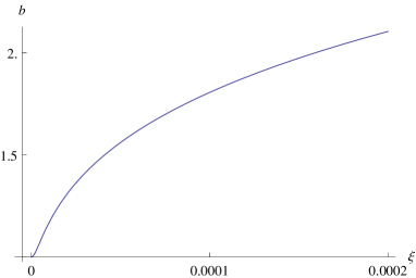
Figure 1: The relation between $b$ and parameter $\xi$.

This string theory background actually introduces another free parameter $\tilde{\kappa}$ into the S-S model and is not dual to the vacuum state of the gauge theory. The same as in [16], the dual state may describe some excited state with (a stochastic averaging of) a constant homogeneous field strength background which gives the expectation value of $tr(F_{\mu\nu}\tilde{F}^{\mu\nu})$

$$\langle tr(F_{\mu\nu}\tilde{F}^{\mu\nu})\rangle=8\pi^{2}N_{c}\tilde{\kappa}\,.$$ (18)

Since the four-dimensional space-time translation invariance and proper Lorentz invariance are preserved in the string background solution, we suppose the dual state is a stochastic average over the background fields in all directions so that the $\langle F\rangle$ is still zero. Obviously the $P$ and $CP$ invariances are violated. This is just similar to the situation in [16] by H. Liu et al. Unlike the D(-1)-D3 background used in [16], the background here is not supersymmetric. The self-duality of the field strength may be related with the supersymmetry. So we cannot say much about the self-duality of the field strength. This state is not the vacuum state of the gauge theory, since in the true vacuum state, $\theta$ should be zero and there is no $\langle tr(F\tilde{F})\rangle$ condensate (as an abuse of terminology, we use “condensate” to denote the expectation value of $tr(F\tilde{F})$ not only in vacuum state but also in the excited state). We assume that there could exist such excited states in the corresponding gauge theory and we are interested in the hadron properties in this kind of states. Such states were proposed to have some possibilities of being created in the heavy ion collisions as we stated in the introduction section. In [34], we have put the Sakai-Sugimoto model in this background and discussed the effects of $\tilde{\kappa}$ on the properties of the low energy Goldstones and mesons. In [41], chiral condensate is studied with finite baryon density in this background. In the next few sections, we will study the $\tilde{\kappa}$ dependence of the baryon mass spectrum in the S-S model.

Now we have some independent parameters on the gravity side: $R^{3}$, $U_{Q0}^{3}$, $U_{KK}$ and $g_{s}$, and $\ell_{s}$ will be cancelled out in the final physical results. We also have some parameters on the gauge theory side $N_{c}$, $M_{KK}$, $\lambda$ and $\tilde{\kappa}$. We have seen that $\tilde{\kappa}$ can be related to $b$ and we can use $b$ to represent $\tilde{\kappa}$. The final results on the gauge theory side can be expressed using $N_{c}$, $M_{KK}$, $\lambda$ and $b$. We collect the relations here:

$$R^{3}=\frac{\lambda\ell_{s}^{2}}{2M_{KK}}\,,\quad g_{s}=\frac{\lambda}{2\pi M_{KK}N_{c}\ell_{s}}\,,\quad U_{KK}=\frac{2}{9}M_{KK}\lambda\ell_{s}^{2}b\,.$$ (19)

We fix the gauge theory parameters $M_{KK}$, $N_{c}$ and $\lambda$, and then vary $\tilde{\kappa}$ to see the effects in the hadron physics. This corresponds to fixing the parameters on the gravity side: $R^{3}$, $g_{s}$, $b/U_{KK}$, and altering $b$ or $U_{KK}$.

Similar to the discussion of the D4-soliton background [Kruczenski:2003uq] in the S-S model, in [34] we also discussed the reliability of the background. We simply state the result here: the valid region of the string theory solution really corresponds to the strong coupling region of the four-dimensional gauge theory in the ’t Hooft limit.

3 Classical soliton solution

After adding $N_{f}$ D8-anti-D8 branes into the D0-D4 system, we have introduced $N_{f}$ flavors and the chiral symmetry $U_{L}(N_{f})\times U_{R}(N_{f})$. The embedding is nontrivial in $\tau-U$ direction, $U(\tau)$. The separated D8 and anti-D8 far away combine near the horizon which corresponds to the spontaneously breaking of $U_{L}(N_{f})\times U_{R}(N_{f})$ symmetry to $U_{V}(N_{f})$ in the field theory and this is verified by the appearance of massless Goldstones[34]. We still choose the antipodal embedding for simplicity of the discussion. Table 1 illustrates the brane configurations.

	0	1	2	3	$4(\tau)$	$5(U)$	6	7	8	9
D4	-	-	-	-	-
D8	-	-	-	-		-	-	-	-	-
D0	$=$	$=$	$=$	$=$	-

Table 1: The brane configurations: “$=$” denotes the smeared directions, “-” denotes the world volume directions.

The induced metric is

$$ds^{2} = \left(\frac{U}{R}\right)^{3/2}H_{0}(U)^{-1/2}\left(f(U)+\left(\frac{R}{U}\right)^{3}\frac{H_{0}(U)}{f(U)}{U^{\prime}}^{2}\right)d\tau^{2}$$ (20)

$$+\left(\frac{U}{R}\right)^{3/2}H_{0}^{1/2}(U)\eta_{\mu\nu}dx^{\mu}dx^{\nu}+H_{0}^{1/2}(U)\left(\frac{R}{U}\right)^{3/2}U^{2}d\Omega_{4}^{2}\,.$$

$U^{\prime}$ is the derivative with respect to $\tau$. We then make the change of the coordinate $U^{3}=U_{KK}^{3}+U_{KK}r^{2}$,

$$y=r\cos\theta\,,\quad z=r\sin\theta.$$ (21)

Then D8 is embedded at $y=0$ and on D8 $U^{3}=U_{KK}^{3}+U_{KK}z^{2}$. Now the induced metric becomes

$$ds_{D8}^{2}= H_{0}^{1/2}(U)\left(\frac{R}{U}\right)^{-3/2}dx^{2}+H_{0}^{1/2}(U)\left(\frac{R}{U}\right)^{3/2}U^{2}d\Omega_{4}^{2}$$

$$+\frac{4}{9}\left(\frac{R}{U}\right)^{3/2}\frac{H_{0}(U_{KK})}{H_{0}^{1/2}(U)}(1-h(r)z^{2})dz^{2}$$ (22)

To discuss the baryons spectrum in the S-S model in the D0-D4 background, we adopt the approach of [37]. The baryon excitations can be viewed as instanton configurations of the gauge field excitations in the $1,2,3,4,z$ directions on the D8-branes. By quantizing the collective coordinates of the instanton, one can obtain the baryon spectrum in presence of $\tilde{\kappa}$.

We start with the low energy effective action of the non-Abelian gauge field on the D8-brane. This action contains two parts: one is from the DBI action

$$S_{\rm YM}=-\tilde{T}U^{-1}_{KK}\int d^{4}xdz\ 2\,H_{0}^{1/2}(U){\rm tr}\left[\frac{1}{4}\frac{R^{3}}{U}{\cal F}_{\mu\nu}{\cal F}^{\mu\nu}+\frac{9}{8}\frac{U^{3}}{U_{KK}}{\cal F}_{z\mu}{\cal F}^{z\mu}\right]$$ (23)

where

$${\tilde{T}}=\frac{(2\pi\alpha^{\prime})^{2}}{3g_{s}}\,T_{8}\,\omega_{4}\,U^{3/2}_{KK}\,R^{3/2}=\frac{M^{2}_{KK}\lambda N_{c}{b}^{3/2}}{486\pi^{3}}$$ (24)

and the other is from the Chern-Simons terms

$$S_{CS} = \frac{N_{c}}{24\pi^{2}}\int_{M^{4}\times R}\omega_{5}({\mathcal{A}})\,,$$ (25)

$$\omega_{5}({\cal A}) = {\rm tr}\left({\cal A}\wedge{\cal F}\wedge{\cal F}-\frac{1}{2}{\cal A}^{3}\wedge{\cal F}+\frac{1}{10}{\cal A}^{5}\right)\,.$$ (26)

The gauge field $\cal A$ and field strength $\cal F$ can be decomposed to a $SU(N_{f})$ part and a $U(1)$ part:

$$\mathcal{A} = \mathcal{A}_{\mu}dx^{\mu}+\mathcal{A}_{z}dx^{z}=A+\frac{1}{\sqrt{2N_{f}}}\hat{A}=A^{a}T^{a}+\frac{1}{\sqrt{2N_{f}}}\hat{A}\,,$$

$$\mathcal{F} = d\mathcal{A}+i\mathcal{A}\wedge\mathcal{A}=F+\frac{1}{\sqrt{2N_{f}}}\hat{F}\,.$$ (27)

To simplify the calculation, we make the replacement $z\to zU_{KK}$, $\mathcal{A}_{z}\to\mathcal{A}_{z}/U_{KK}$, $x_{\mu}\to x_{\mu}/M_{KK}$, $\mathcal{A}_{\mu}\to\mathcal{A}_{\mu}M_{KK}$ to work with dimensionless $x$, $z$ and $\mathcal{A}_{\mu}$, $\mathcal{A}_{z}$. The Chern-Simons terms are not affected and the Yang-Mills action changes to

$$S_{\rm YM} =-\tilde{T}M^{-2}_{KK}\frac{9}{4b}\int d^{4}xdz\ H_{0}^{1/2}(U){\rm tr}\left[\frac{1}{2}\frac{U_{KK}}{U}{\cal F}_{\mu\nu}{\cal F}^{\mu\nu}+\frac{U^{3}}{U^{3}_{KK}}b{\cal F}_{z\mu}{\cal F}^{z\mu}\right],$$ (28)

$$=-a\lambda N_{c}b^{1/2}\int d^{4}xdz\ H_{0}^{1/2}(U){\rm tr}\left[\frac{1}{2}K(z)^{-1/3}{\cal F}_{\mu\nu}{\cal F}^{\mu\nu}+K(z)b{\cal F}_{z\mu}{\cal F}^{z\mu}\right],$$ (29)

where $a=\frac{1}{216\pi^{3}}$, and $K(z)=1+z^{2}$. To use $U_{KK}$ to make $z$ and $A_{z}$ dimensionless is to keep the coefficient of the second term finite in the $\ell_{s}\to 0$ limit. We can then make another change of coordinate $z\to b^{1/2}z$, $A_{z}\to A_{z}/b^{1/2}$, to give the standard normalization of the second term:

$$S_{\rm YM} =-a\lambda N_{c}b\int d^{4}xdz\ \,H_{0}^{1/2}(U){\rm tr}\left[\frac{1}{2}K(zb^{1/2})^{-1/3}{\cal F}_{\mu\nu}{\cal F}^{\mu\nu}+K(zb^{1/2}){\cal F}_{z\mu}{\cal F}^{z\mu}\right],$$ (30)

The integrand is different from the original one in [37] by $b$ factors inside $K$ and the overall factor $H^{1/2}_{0}(U)$.

By the same reasoning as in [37], since we are working in the large $\lambda$ region, we can make a $1/\lambda$ expansion. It is convenient to make another rescaling of the coordinates and ${\cal A}_{M}$,

$$x^{0}\to x^{0} \quad x^{M}\to\lambda^{-1/2}x^{M}$$ ,

$$\mathcal{A}_{0}(t,x)\to{\mathcal{A}}_{0}(t,x) \quad\mathcal{A}_{M}(t,x)\to\lambda^{1/2}{\mathcal{A}}_{M}(t,x)$$ ,

$$\mathcal{F}_{0M}(t,x)\to\lambda^{1/2}{\mathcal{F}}_{0M}(t,x) \quad\mathcal{F}_{MN}(t,x)\to\lambda{\mathcal{F}}_{MN}(t,x)\,,$$ , (31)

where $M,N=1,2,3,z$. Expanding the Lagrangian with respect to $1/\lambda$, and keeping terms to $O(\lambda^{0})$, we have

$$S_{\rm YM}=-aN_{c}b^{3/2}\int d^{4}xdz \left[\frac{\lambda}{4}(F^{a}_{MN})^{2}-\frac{b\,z^{2}}{2}(\frac{5}{12}-\frac{1}{4b})(F^{a}_{ij})^{2}+\frac{b\,z^{2}}{4}(1+\frac{1}{b})(F^{a}_{iz})^{2}-\frac{1}{2}(F^{a}_{0N})^{2}\right.$$

$$\left.+\frac{\lambda}{4}\hat{F}^{2}_{MN}-\frac{b\,z^{2}}{2}(\frac{5}{12}-\frac{1}{4b})\hat{F}^{2}_{ij}+\frac{b\,z^{2}}{4}(1+\frac{1}{b})\hat{F}^{2}_{iz}-\frac{1}{2}\hat{F}^{2}_{0N}+O(\lambda^{-1})\right]$$ (32)

with $i=1,2,3$. For simplicity we are now working with only two flavors, that is $N_{f}=2$. We have decomposed the gauge field into the $SU(2)$ and $U(1)$ parts as in (27). The Chern-Simons action can also be decomposed as

$$S_{CS}= \frac{N_{c}}{24\pi^{2}}\epsilon_{MNPQ}\int d^{4}xdz[\frac{3}{8}\hat{A_{0}}tr(F_{MN}F_{PQ})-\frac{3}{2}\hat{A}_{M}tr(\partial_{0}A_{N}F_{PQ})$$

$$+\frac{3}{4}\hat{F}_{MN}tr(A_{0}F_{PQ})+\frac{1}{16}\hat{A}_{0}\hat{F}_{MN}\hat{F}_{PQ}-\frac{1}{4}\hat{A}_{M}\hat{F}_{0N}\hat{F}_{PQ}+(...)]$$ (33)

The ellipsis denotes some total derivative terms. The EOM for the gauge fields can then be obtained up to $O(\lambda^{-1})$:

$$D_{M}F_{MN}=0\,,\quad D_{M}F^{a}_{0M}+\frac{\epsilon_{MNPQ}}{64\pi^{2}ab^{3/2}}\hat{F}_{MN}F^{a}_{PQ}=0$$ (34)

$$\partial_{M}\hat{F}_{MN}=0\,,\quad\partial_{M}\hat{F}_{0M}+\frac{\epsilon_{MNPQ}}{128\pi^{2}ab^{3/2}}F^{a}_{MN}F^{a}_{PQ}=0$$ (35)

$\frac{1}{2}\hat{A}_{0}$ is coupled to the quark number operator and the instanton number $n=\frac{1}{32\pi^{2}}\epsilon_{MNPQ}\int d^{4}xtr(F_{MN}F_{PQ})$ is just the baryon number. The BPST one-instanton solution of the EOM of $F_{MN}$ is equivalent to the Skyrmion description of a baryon,

$$A_{M}=-if(\xi)g^{-1}(x)\partial_{M}g(x),$$

$$f(\xi)=\frac{\xi^{2}}{\xi^{2}+\rho^{2}},\quad \xi^{2}=(\vec{x}-\vec{X})^{2}+(z-Z)^{2},\quad g(x)=\frac{1}{\xi}((z-Z)-i(\vec{x}-\vec{X})\cdot\vec{\sigma})\,,$$ (36)

where $\vec{\sigma}$ are the Pauli matrices. The EOM of the $U(1)$ $\hat{A}_{M}$ gives the solution $\hat{A}_{M}=0$ up to a gauge transformation. The equation for $A_{0}$ then becomes $D_{M}^{2}A_{0}=0$. The same as the argument in [37], the solution with vanishing boundary condition at infinity is given by $A_{0}=0$. Inserting the BPST solution into the EOM of $\hat{A}_{0}$, we have

$$-\partial_{M}^{2}\hat{A}_{0}+\frac{3\rho^{4}}{\pi^{2}ab^{3/2}(\xi^{2}+\rho^{2})^{4}}=0$$ (37)

and the solution is

$$\hat{A}_{0}=-\frac{1}{8\pi^{2}ab^{3/2}}\frac{\xi^{2}+2\rho^{2}}{(\rho^{2}+\xi^{2})^{2}}\,.$$ (38)

Substituting this solution into the action, we obtain the soliton mass from the on-shell action $S=-\int dtM$:

$$M = 8\pi^{2}ab^{3/2}N_{c}\left(\lambda+\frac{1}{12}(3-b)(2Z^{2}+\rho^{2})+\frac{1}{320\pi^{4}\rho^{2}a^{2}b^{3}}+O\Big{(}\frac{1}{\lambda}\Big{)}\right)$$ (39)

If $b<3$, we can find out the minimum of $M$ at $\rho_{min}$ which characterize the size of the baryon:

$$\rho^{2}_{min}=\frac{1}{4\pi^{2}}\sqrt{\frac{3}{5}}\frac{1}{ab^{3/2}\sqrt{3-b}}\,.$$ (40)

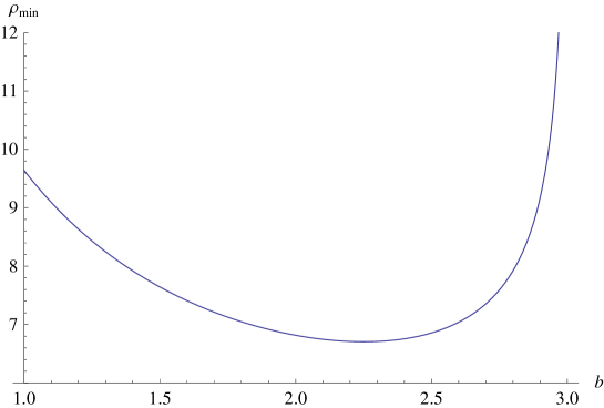
Figure 2: The change of the size of the baryon $\rho_{min}$ with respect to $b$.

Inserting $\rho_{min}$ into $M$, we have the minimum of the soliton mass,

$$M_{min}=8\pi^{2}ab^{3/2}N_{c}\left(\lambda+9\pi\sqrt{\frac{3}{5}}\frac{\sqrt{3-b}}{b^{3/2}}+\frac{1}{6}(3-b)Z^{2}+O\Big{(}\frac{1}{\lambda}\Big{)}\right)\,.$$ (41)

From figure (2) we see that the size goes down first as $b$ increases and grows and blow up as $b\to 3$. We define $b_{min}=9/4$ at which $\rho_{min}$ is the minimum. At $b=3$, the second term of (41) vanishes and it is obvious that $\rho_{min}$ goes to infinity if we ignore $O(1/\lambda)$ terms.

However, we have to estimate the region of $b$ for which the $1/\lambda$ expansion of the action to $O(\lambda^{0})$ is good. The $O(\lambda^{0})$ terms, i.e., the second and the third terms in the bracket in (41), are monotonically decreasing for $1<b<3$. So if for $b=1$ the $O(\lambda^{0})$ term is smaller than $\lambda$, it will be so for all $1<b<3$. We can estimate the value: at $b=1$, for $Z=0$, the second term is $9\sqrt{\frac{6}{5}}\pi\simeq 31$. So it is enough to choose the $\lambda$ to be larger than $10^{2}$ to have $O(\lambda^{0})$ terms smaller than the $O(\lambda)$ term. From (17) and (16), we have a constraint for $\xi$ and $b$, $\xi<10^{-4}$ for $\lambda=100$ and $1<b<1.81$ for $\tilde{\kappa}<M_{KK}^{4}$ if we do not consider massive modes. However, for fixed $\lambda$, as $b$ approaching 3, $\rho_{min}^{2}$ goes to infinity and larger than $\lambda$, and the $1/\lambda$ expansion may not be a good approximation at such a large $\rho$. It is hard to estimate the range $b$ for which the expansion is good. We will use an operative estimation as follows. The second term which is divergent for $\rho\to\infty$ in the bracket of (39) comes from the integral of the static BPST solution. So we could evaluate $S_{\rm YM}$ in (30) using BPST solution numerically at $\rho_{min}$ with $\hat{A}_{0}=0$ and compare it with (32) which is the $1/\lambda$ expansion of the same integral. See figure 3 for illustration of the differences. We can see that near $b=3$ the differences become divergent because $\rho_{min}\to\infty$ for $b\to 3$. Since the evaluation of the integration (30) partly takes account of higher order $O(1/\lambda)$ contributions, we would expect the difference should be smaller than the $O(\lambda^{0})$ terms in order to have a good approximation. This requirement puts a constraint on the range of $b$. For $\lambda\sim 10^{2}$, this will give a rough constraint $1<b<1.5$ which is within the above $1<b<1.81$. For $\lambda\sim 250$, this will give a constraint about $1<b<1.8$. But (17) and (16) give a constraint $1<b<1.25$. In $1.25<b<1.8$, we would expect that the massive modes of the gauge theory come into play. In general, equations (17) and (16) require that the larger $\lambda$ is, the smaller the region for $b$ is for $\tilde{\kappa}<M_{KK}^{4}$. The above criterion for a good $O(\lambda^{0})$ approximation requires the opposite, that is, the larger $\lambda$ is, the larger the region for $b$ is.

Above we consider the expansion of $S_{\rm YM}$ from BPST part to be a good expansion. If we also include the $\hat{A}_{0}$ contributions, there are some subtleties to be considered. Recall that, in [34] when we consider the condition that $e^{\Phi}\ll 1$ which is needed for the suppression of the string loop effects, we need $UH_{0}(U)\ll g_{s}^{-4/3}R$, and from (19) we have

$$\frac{U}{U_{KK}}=(1+z^{2}b/\lambda)^{1/3}\ll\frac{9\pi^{4/3}N_{c}^{4/3}}{\lambda^{2}b}\,.$$ (42)

Though we are working in the large $N_{c}$ limit and the right hand side of (42) can be arbitrarily large, to do numerical computation, we have to fix a finite $N_{c}$. Then (42) gives a constraint for the value of $z$ and thus introduces a cut-off of the integration over $z$. This does not affect the integral of BPST part since the integral converges quickly such that the variation of limits of $z$ integration does not change the result too much, as long as the integration limits are large enough. But since $\hat{F}_{0z}^{2}\sim 1/\xi^{6}$ for large $z$ and the $O(\lambda^{-1})$ term of $k(z)$ is proportional to $z^{2}$, the second term in (29) does not have a good convergent property. We have to choose the integration cut-off of $z$ to have a good $1/\lambda$ expansion to $O(\lambda^{0})$. So the integration limits cannot be chosen arbitrarily large. By numerical test, we find out that the choice for the limits of $z$ integration to be of $O(\lambda/10)$ is a good one. And this does not change the results in previous paragraph. We can then look at how large the $N_{c}$ should be from (42), that is $N_{c}\gg\frac{\lambda^{3/2}b^{3/4}}{3^{3/2}\pi}(1+\frac{z^{2}b}{\lambda})^{1/4}$. If we choose $\lambda=10^{2}$ and $z=\lambda/10=10$, $N_{c}\gg 10^{2}$ for $b\in(1,1.5)$. For $\lambda\gg 10^{2}$ and $z\sim\lambda/10$, $N_{c}\gg\frac{\lambda^{7/4}b}{\sqrt{270}\pi}\sim 0.02b\lambda^{7/4}$. So $N_{c}$ should be rather large for the $1/\lambda$ expansion to be good.

Now we can see that adding the condensate will cause the baryon to shrink for small $\tilde{\kappa}$. From (39) the second term is an attractive potential and the third term is a repulsive one. For small $b$ near $b=1$, the attractive potential [including the $b^{3/2}$ factor before the bracket in (39) ] grows while the repulsive one decreases as $b$ increases. So it can be understood that the baryon size shrinks as $b$ increases. For larger $b$, the attractive potential also decreases and the repulsive one decreases more slowly with increasing $b$. At $b>b_{min}$ which corresponds to larger $\tilde{\kappa}$ , we can always choose $\lambda$ large enough to make the $1/\lambda$ expansion a good approximation to $O(\lambda^{0})$. At such $b$, the repulsive force will be decreasing more slowly than the attractive force and the radius will be increasing with $b$. However, in this case, $\tilde{\kappa}$ is always greater than $M^{4}_{KK}$ for our chosen $\lambda>100$, and the massive modes, including fermions, bosons and KK modes from the five-dimensional gauge theory, may come into play.

Figure 3: The integral of $S_{\rm YM}$: the solid line denotes the one not expanded with respected to $1/\lambda$ and the dashed line the one expanded to $O(\lambda^{0})$. The left figure is for $\lambda=100$ and the right one for $\lambda=250$.

4 Quantization of the collective modes and the spectrum for baryons

The BPST instanton solution are parametrized by position $\vec{X}$, $Z$, size $\rho$, and together with the global $SU(2)$ orientation parametrized by three independent $SU(2)$ parameters, $a_{I}$, $(I=1,2,3,4)$ with $\sum_{I}a_{I}^{2}=1$, they form the moduli space of the one-instanton solution, $\mathcal{M}=\mathbb{R}^{4}\times\mathbb{R}^{4}/\mathbb{Z}_{2}$. As in [37], we also define $y_{I}$, $I=1,2,3,4$ to combine $\rho$, $a_{I}$, with $\sum_{I}y_{I}^{2}=\rho^{2}$ and $a_{I}=y_{I}/\rho$. The basic idea to study the baryon spectrum in the approach of [37] is to regard the soliton as a slowly moving particle described by time-dependent collective coordinates. The motion of the particle can be quantized, and the energy spectrum can be obtained by the eigenvalues of the Hamiltonian for the collective coordinates.

First, we promote the coordinates to be time dependent: the positions $\vec{X}(t)$, $Z(t)$, the size $\rho(t)$, $SU(2)$ orientation $a_{I}(t)$, or collectively denoted by $X^{\alpha}=(\vec{X}(t),Z(t),y_{I}(t))$. The $SU(2)$ gauge field becomes time dependent,

$$A_{M}(t,x)=VA_{M}^{cl}(x,X^{\alpha}(t))V^{-1}-iV\partial_{M}V^{-1}.$$ (43)

where $A_{M}^{cl}(x,X^{\alpha})$ is the BPST instanton solution with $\vec{X}$, $Z$, $\rho$ replaced by time-dependent ones. $V(x,t)$ is a $SU(2)$ $2\times 2$ matrix which is asymptotic to $\mathbf{a}=a_{4}(t)+ia_{a}(t)\sigma^{a}$ at $z\to\infty$, where $\sigma^{a}$, $a=1,2,3$ are Pauli matrices. The field strength then becomes

$$F_{MN}=VF_{MN}^{cl}V^{-1}\,,\quad F_{0M}=V(\dot{X}^{\alpha}\partial_{\alpha}A_{M}^{cl}-D_{M}^{cl}\phi)V^{-1}$$ (44)

where $\Phi=-iV^{-1}\dot{V}$. The dot denotes the derivative with respect to $t$, i.e., $\partial_{0}$, and $\partial_{\alpha}$ is the derivative with respect to collective coordinates $X^{\alpha}$. $D_{M}$ is the covariant derivative $D_{M}=\partial_{M}+i[A_{M}^{cl},\ ]$, using BPST solution $A^{cl}_{M}$. $F_{MN}$ automatically satisfies the EOM of the first equation in (34). $F_{0M}$ and $\hat{F}_{0M}$ have to satisfy the second equations in (34) and (35). By the analysis in [37], the solution of $A_{0}$ is the same as in [37] and we would not repeat it here. The solution of $\hat{A}_{0}$ is just (38) with collective coordinates replaced by the time-dependent ones.

The motion of the collective coordinates can be characterized by the Lagrangian up to $O(1/\lambda)$ obtained by substituting the time-dependent solution into (32) and (33):

$$L = \frac{1}{2}m_{X}g_{\alpha\beta}\dot{X}^{\alpha}\dot{X}^{\beta}-U(X^{\alpha})$$ (45)

$$= \frac{1}{2}m_{X}\dot{\vec{X}}^{2}+\frac{1}{2}m_{Z}\dot{Z}^{2}+\frac{1}{2}m_{y}\dot{y}_{I}\dot{y}_{I}-U(X^{\alpha})$$ (46)

where $g_{\alpha\beta}$ is the metric for the instanton moduli $ds^{2}=g_{\alpha\beta}dX^{\alpha}dX^{\beta}=d\vec{X}^{2}+dZ^{2}+2dy_{I}^{2}$, and $m_{X}=m_{Z}=\frac{1}{2}m_{y}=8\pi^{2}ab^{3/2}N_{c}$. The potential $U(X)$ is the same as (39) except that the collective coordinates are time dependent. The Hamiltonian can then be obtained:

$$H = H_{X}+H_{Z}+H_{y}\,,$$

$$H_{X} = \frac{1}{2}m_{X}\dot{X}^{i}\dot{X}^{i}+8\pi^{2}\lambda ab^{3/2}N_{c}=\frac{1}{2m_{X}}P_{X}^{2}+M_{0}\,,$$ (47)

$$H_{Z} = \frac{1}{2}m_{Z}\dot{Z}^{2}+\frac{4\pi^{2}}{3}ab^{3/2}(3-b)N_{c}Z^{2}=\frac{1}{2m_{Z}}P_{Z}^{2}+\frac{1}{2}m_{Z}\omega_{Z}^{2}Z^{2}$$ (48)

$$H_{y} = \frac{1}{2}m_{y}\dot{y}_{I}\dot{y}_{I}+\frac{2\pi^{2}}{3}ab^{3/2}(3-b)N_{c}\rho^{2}+\frac{N_{c}}{40\pi^{2}ab^{3/2}}\frac{1}{\rho^{2}}$$ (49)

$$= \frac{1}{2m_{y}}P_{y}^{2}+\frac{1}{2}m_{y}\omega_{y}^{2}\rho^{2}+\frac{Q}{\rho^{2}}\,.$$

We have defined $M_{0}=8\pi^{2}\lambda ab^{3/2}N_{c}$, $\omega_{Z}=\frac{1}{3}(3-b)$, $\omega_{y}=\frac{1}{12}(3-b)$ and $Q=\frac{N_{c}}{40\pi^{2}ab^{3/2}}$, and the momentum $P_{X}$, $P_{Z}$, $P_{y}$ follow the standard definition as the conjugate of the collective coordinates.

We quantize the soliton at rest to obtain the baryon spectrum. The quantization procedure is to replace the momenta in the Hamiltonian to the corresponding differential operators which act on the normalizable wave function describing the motion of the soliton

$$H_{Z} = -\frac{1}{2m_{Z}}\frac{\partial^{2}}{\partial Z^{2}}+\frac{1}{2}m_{Z}\omega_{Z}^{2}Z^{2}$$ (50)

$$H_{y} = -\frac{1}{2m_{y}}\frac{\partial^{2}}{\partial y_{I}^{2}}+\frac{1}{2}m_{y}\omega_{y}^{2}\rho^{2}+\frac{Q}{\rho^{2}}\,.$$ (51)

For the wave function to describe fermions, we need to impose antiperiodic boundary condition: $\psi(-a_{I})=-\psi(a_{I})$. The Hamiltonian is almost the same as the one in [37] only with redefined $m_{Z}$, $m_{y}$, $\omega_{Z}$, $\omega_{y}$ and $Q$. So we can use their result directly,

$$M = M_{0}+E_{y}+E_{Z}\,,\quad M_{0}=\frac{\lambda N_{c}b^{3/2}}{27\pi}$$ (52)

$$E_{y} = \omega_{y}(\tilde{l}+2n_{\rho}+2)=\omega_{y}(\sqrt{(l+1)^{2}+2m_{y}Q}+2n_{\rho}+1)$$ (53)

$$= \frac{1}{2\sqrt{3}}\sqrt{3-b}\left(\sqrt{(l+1)^{2}+\frac{4}{5}N_{c}^{2}}+2n_{\rho}+1\right)\,,$$

$$E_{Z} = \omega_{Z}(n_{z}+\frac{1}{2})=\frac{1}{\sqrt{3}}\sqrt{3-b}(n_{z}+\frac{1}{2})$$ (54)

where $l=1,3,5,\dots$, $n_{\rho}=0,1,2,3,\dots$, and $n_{z}=0,1,2,\dots$. That $l$ takes odd integers is the requirement of the antiperiodic boundary condition of the wave function.

Now we have the baryon mass spectrum. However, there is some uncertainty in the formula. As noted in [37] the $O(N_{c}^{0})$ contribution from $M_{0}$ is ignored which is the same $N_{c}$ order of the zero-point energy in (53) and (54). And the contributions to the zero-point energy from the heavy massive mode excitations around the instanton are also ignored. The sum of these zero-point energy may give a divergent contribution and need be subtracted by the vacuum energy to make it finite. These contributions in general will also depend on $b$. So the $b$ dependence of $M_{0}$ together with all the other zero-point energy contributions cannot be estimated at this stage. If we insisted the large $N_{c}$ and large $\lambda$ expansions to be good approximations, the $O(N_{c}^{0})$ and $O(\lambda^{0})$ contribution from the zero-point energy should not be dominant over $M_{0}$ which is $O(\lambda N_{c})$. However, this may not be realistic for $N_{c}=3$ and the real $\lambda$. Considering such uncertainty, what we can do is to discuss the mass difference between baryon excitation states.

From (53) and (54), we can easily separate the $b$ dependence in $E_{y}$ and $E_{Z}$:

$$M=M_{0}+\sqrt{\frac{3-b}{2}}\big{(}E_{y}(b=1)+E_{Z}(b=1)\big{)},\quad\Delta M=\sqrt{\frac{3-b}{2}}\Delta M(b=1)$$ (55)

So, the difference between two baryon states is proportional to $\sqrt{3-b}$. For $1<b<3$, the difference become smaller as $b$ increases and disappears at $b=3$. This result is independent of the specific properties such as spin or isospin of the baryons. However, as discussed in section 3, the suitable region of $b$ for our method is constrained by the $1/\lambda$ approximation. For $\lambda\sim 100$, only $1<b<1.5$ could give a good $1/\lambda$ approximation to $O(1)$ and in this region $\tilde{\kappa}<M_{KK}^{4}$. The massive modes of the gauge theory decouples. For $\lambda$ large enough, $b$ can be near $3$ with good $1/\lambda$ approximation but $\tilde{\kappa}$ can be greater than $M^{4}_{KK}$. So the behavior of $M$ for such large $b$ has already included the contributions from the massive modes in the gauge theory. If we are only interested in the contribution of the massless gauge field, we cannot trust the large $b$ region and cannot say much about the behavior in this region. However, near $b=1$, the qualitative behavior of result above can be trusted.

5 Conclusion and discussion

We have discussed the baryon spectrum in the S-S model with smeared D0 charge turned on in the D4-soliton background. The D0-D4 background corresponds to an excited state with $\tilde{\kappa}$ which is proportional to a nonzero $tr(F_{\mu\nu}\tilde{F}^{\mu\nu})$. The dependence on $\tilde{\kappa}$ is through a parameter $b$, which is monotonically increasing with $\tilde{\kappa}$. We follow the method in [37], in which the static baryon is represented by an instanton solution and by quantizing the collective coordinates, one can obtain the baryon spectrum.

In the classical analysis, for $b<3$, the soliton mass has an attractive potential and a repulsive potential. For small $\tilde{\kappa}$, the attractive potential grows with $\tilde{\kappa}$ and the repulsive potential decreases. This causes the size of the baryon to shrink. For larger $\tilde{\kappa}$, the massive modes in the gauge theory may also come into play, and the size of the baryon will grow with $\tilde{\kappa}$. It may be possible that as we increase the $\lambda$, the upper bound for $b$ goes closer to $3$ according to our criterion, and the radius really grows larger and larger such that the baryon breaks up. In this case, more and more KK modes come in and may play a role in driving the baryon unstable. However, our criterion for the $1/\lambda$ approximation may not be applicable for $b$ very close to $3$. This is because the integration we used in the criterion only counts in parts of the $O(1/\lambda)$ contributions, and the other $O(1/\lambda)$ contributions can be comparably larger than the $O(\lambda^{0})$ terms near $b=3$ in (39) in which the $O(\lambda^{0})$ terms is exact zero at $b=3$ for finite $\rho$ and $Z$. This is partly the reason for the divergence of the radius in (40) at $b=3$ to $O(\lambda^{0})$. In this case, we cannot say anything near $b=3$ in our present approximation. Nevertheless, for $b>3$, the $O(\lambda^{0})$ term is negative and nonzero which means a repulsive potential. We can choose large enough $\lambda$ so that $O(\lambda^{0})$ dominate the higher order terms at finite $\rho$ and $Z$. Obviously, the baryon cannot be formed with only repulsive force. So, this also indicates a possibililty that for large enough $\lambda$ and $b$ where the massive KK modes contribute, the baryons cannot exist.

In the analysis of the baryon spectrum by quantization of collective coordinates, the zero-point energy cannot be estimated by the present method. So what we can consider is the difference between baryon masses. The dependence of the mass difference on the $\tilde{\kappa}$ is simply $\sqrt{\frac{3-b}{2}}\Delta M(b=1)$ and the factor is independent of the spin and isospin. So with $\tilde{\kappa}$ turned on the mass difference between baryons will be smaller. For $b>3$, the baryon masses become complex which also indicates that they cannot be stable. This is not surprising since the repulsive potential in the classical analysis of the previous paragraph is used here in the Schödinger equation. So, as long as the large $\lambda$ expansion is applicable for some region in $b>3$, we conclude that the baryons cannot exist in this region. However, at this region $\tilde{\kappa}>M_{KK}^{4}$, contribution from the massive KK modes of the gauge theory should be counted in. Though this may not be the property of the low energy QCD, it is a property of the world volume theory of the D4 compactified on a circle.

As we learned from the study in [34], the mass spectra of the mesons and the interactions between mesons do depend on $\tilde{\kappa}$, which means that $\tilde{\kappa}$ really affects the interactions between quarks. But this effect is not so drastic as to endanger the stability of mesons there; however, in the present paper strong $\tilde{\kappa}$ does destroy baryons. This may be qualitatively explained as follows: a baryon is formed by $N_{c}$ quarks while a meson is only formed by a quark-antiquark pair. Since we are discussing in the large $N_{c}$ region, a baryon may consist of a large number of quarks. It is not surprising that the total effect of $\tilde{\kappa}$ on the interactions among such a large number of quarks should be much larger than the effect on only one pair of quark and antiquark which forms a meson, and even large enough to destabilize the baryons. As for the chiral symmetry breaking, it is characterized by the $\bar{q}q$ condensate, which involves only two quark fields $q$. So similar to the meson cases, from the study in [34], $\tilde{\kappa}$ effect is too small to demolish chiral symmetry breaking. From a geometric point of view in the S-S model, the spontaneous chiral symmetry breaking is realized as the merging of the D8-brane and anti-D8-brane. So, as long as this kind of geometry is present and it is a valid dual description of the field theory, the spontaneous chiral symmetry breaking is expected to be there. For the geometry to be valid, $b$ cannot be arbitrarily large which can be seen from (42) for fixed $N_{c}$ and $\lambda$.

As in most gauge-gravity dual analysis, our analysis is done in the large $N_{c}$ limit and large ’t Hooft coupling region. Since the baryon spectrum demonstrates the right large $N_{c}$ behavior as in [37], we expect that the model also captures the qualitative $\tilde{\kappa}$ behavior at least for small $\tilde{\kappa}$ for QCD-like theory at large $N_{c}$ with large $\lambda$. We have estimated that $\lambda$ should roughly be larger than $10^{2}$, and $N_{c}$ should also be rather large according to the discussion in section 3. This also applies to the original discussion on baryons in the S-S model with $\tilde{\kappa}=0$ in [37]. Although in [37], the authors did compared the result with the experiments with $N_{c}=3$ heuristically, it should be understood that it is still a long way to the realistic $N_{c}$ and $\lambda$.

References

- [1] D. Kharzeev, R. D. Pisarski and M. H. G. Tytgat, Phys. Rev. Lett. 81 (1998) 512 [hep-ph/9804221]; hep-ph/9808366; [hep-ph/0012012].
- [2] K. Buckley, T. Fugleberg and A. Zhitnitsky, Phys. Rev. Lett. 84 (2000) 4814 [hep-ph/9910229].
- [3] D. Kharzeev, Phys. Lett. B 633 (2006) 260 [hep-ph/0406125].
- [4] E. V. Shuryak and A. R. Zhitnitsky, Phys. Rev. C 66, 034905 (2002) [hep-ph/0111352].
- [5] D. E. Kharzeev, L. D. McLerran and H. J. Warringa, Nucl. Phys. A 803, 227 (2008) [arXiv:0711.0950 [hep-ph]].
- [6] K. Fukushima, D. E. Kharzeev and H. J. Warringa, Phys. Rev. D 78, 074033 (2008) [arXiv:0808.3382 [hep-ph]].
- [7] D. E. Kharzeev, Prog. Part. Nucl. Phys. 75, 133 (2014) [arXiv:1312.3348 [hep-ph]].
- [8] Yu. A. Simonov, Phys. Usp. 39 (1996) 313 [Usp. Fiz. Nauk 166 (1996) 337] [hep-ph/9709344].
- [9] H. Leutwyler, Phys. Lett. B 96 (1980) 154; Nucl. Phys. B 179 (1981) 129.
- [10] P. Minkowski, Nucl. Phys. B 177 (1981) 203.
- [11] C. A. Flory, Phys. Rev. D 28 (1983) 1425.
- [12] P. van Baal, Commun. Math. Phys. 94 (1984) 397.
- [13] G. V. Efimov, A. C. Kalloniatis and S. N. Nedelko, Phys. Rev. D 59 (1998) 014026 [hep-th/9806165].
- [14] J. Ambjorn and P. Olesen, Nucl. Phys. B 170, 60 (1980).
- [15] P. A. Amundsen and M. Schaden, Phys. Lett. B 252, 265 (1990).
- [16] H. Liu and A. A. Tseytlin, Nucl. Phys. B 553 (1999) 231 [hep-th/9903091].
- [17] A. Kehagias and K. Sfetsos, Phys. Lett. B 456 (1999) 22 [hep-th/9903109].
- [18] K. Ghoroku and M. Yahiro, Phys. Lett. B 604 (2004) 235 [hep-th/0408040].
- [19] K. Ghoroku, T. Sakaguchi, N. Uekusa and M. Yahiro, Phys. Rev. D 71 (2005) 106002 [hep-th/0502088].
- [20] I. H. Brevik, K. Ghoroku, A. Nakamura, Int. J. Mod. Phys. D 15 (2006) 57 [hep-th/0505057].
- [21] K. Ghoroku, M. Ishihara and A. Nakamura, Phys. Rev. D 74 (2006) 124020 [hep-th/0609152].
- [22] J. Erdmenger, K. Ghoroku and I. Kirsch, JHEP 0709 (2007) 111 [arXiv:0706.3978 [hep-th]].
- [23] J. Erdmenger, A. Gorsky, P. N. Kopnin, A. Krikun and A. V. Zayakin, JHEP 1103 (2011) 044 [arXiv:1101.1586 [hep-th]].
- [24] K. Ghoroku and M. Ishihara, Phys. Rev. D 77 (2008) 086003 [arXiv:0801.4216 [hep-th]].
- [25] K. Ghoroku, M. Ishihara, A. Nakamura and F. Toyoda, Phys. Rev. D 79 (2009) 066009 [arXiv:0806.0195 [hep-th]].
- [26] S. -J. Sin, S. Yang and Y. Zhou, JHEP 0911 (2009) 001 [arXiv:0907.1732 [hep-th]].
- [27] B. Gwak, M. Kim, B. -H. Lee, Y. Seo and S. -J. Sin, Phys. Rev. D 86 (2012) 026010 [arXiv:1203.4883 [hep-th]].
- [28] S. -J. Sin and Y. Zhou, JHEP 0905 (2009) 044 [arXiv:0904.4249 [hep-th]].
- [29] E. Witten, Adv. Theor. Math. Phys. 2 (1998) 505 [hep-th/9803131].
- [30] T. Sakai and S. Sugimoto, Prog. Theor. Phys. 113 (2005) 843 [hep-th/0412141].
- [31] T. Sakai and S. Sugimoto, Prog. Theor. Phys. 114 (2005) 1083 [hep-th/0507073].
- [32] J. L. F. Barbón and A. Pasquinucci, Phys. Lett. B 458 (1999) 288 [hep-th/9904190].
- [33] K. Suzuki, Phys. Rev. D 63 (2001) 084011 [hep-th/0001057].
- [34] C. Wu, Z. Xiao and D. Zhou, Phys. Rev. D 88, no. 2, 026016 (2013) [arXiv:1304.2111 [hep-th]].
- [35] E. Bergshoeff, A. Collinucci, A. Ploegh, S. Vandoren and T. Van Riet, JHEP 0601 (2006) 061 [hep-th/0510048].
- [36] K. Nawa, H. Suganuma and T. Kojo, Phys. Rev. D 75, 086003 (2007) [hep-th/0612187].
- [37] H. Hata, T. Sakai, S. Sugimoto and S. Yamato, Prog. Theor. Phys. 117 (2007) 1157 [hep-th/0701280 [HEP-TH]].
- [38] K. Hashimoto, T. Sakai and S. Sugimoto, Prog. Theor. Phys. 120 (2008) 1093 [arXiv:0806.3122 [hep-th]].
- [39] K. Hashimoto, T. Sakai and S. Sugimoto, Prog. Theor. Phys. 122 (2009) 427 [arXiv:0901.4449 [hep-th]].
- [40] V. Kaplunovsky and J. Sonnenschein, JHEP 1105 (2011) 058 [arXiv:1003.2621 [hep-th]].
- [41] S. Seki and S. -J. Sin, JHEP 1310, 223 (2013) [arXiv:1304.7097 [hep-th]].