Indirect constraints on the Georgi-Machacek model and implications for Higgs couplings
Abstract
We update the indirect constraints on the Georgi-Machacek model from -physics and electroweak precision observables, including new constraints from and . We illustrate the effect of these constraints on the couplings of the Standard Model-like Higgs boson by performing scans using the most general scalar potential, subject to vacuum stability and perturbativity constraints. We find that simultaneous enhancements of all the Higgs production cross sections by up to 39% are still allowed after imposing these constraints. LHC rate measurements on the Higgs pole could be blind to these enhancements if unobserved non-standard Higgs decays are present.
I Introduction
Since the 2012 discovery of a Standard Model (SM)-like Higgs boson at the CERN Large Hadron Collider (LHC) Aad:2012tfa , there has been considerable interest in models with extended Higgs sectors to be used as benchmarks for LHC searches for physics beyond the SM. One such model is the Georgi-Machacek (GM) model Georgi:1985nv ; Chanowitz:1985ug , which adds isospin-triplet scalar fields to the SM in a way that preserves custodial SU(2) symmetry. Its phenomenology has been extensively studied Gunion:1989ci ; Gunion:1990dt ; HHG ; Haber:1999zh ; Aoki:2007ah ; Godfrey:2010qb ; Low:2010jp ; Logan:2010en ; Falkowski:2012vh ; Chang:2012gn ; Carmi:2012in ; Chiang:2012cn ; Chiang:2013rua ; Kanemura:2013mc ; Englert:2013zpa ; Killick:2013mya ; Belanger:2013xza ; Englert:2013wga ; Efrati:2014uta ; HKL ; Chiang:2014hia ; Chiang:2014bia ; Godunov:2014waa . The GM model has also been incorporated into the scalar sectors of little Higgs Chang:2003un ; Chang:2003zn and supersymmetric Cort:2013foa ; Garcia-Pepin:2014yfa models, and an extension with an additional isospin doublet Hedri:2013wea has also been considered.
The GM model has the interesting feature that the coupling strengths of the SM-like Higgs boson to or boson pairs can be larger than in the SM.111An enhancement of the and couplings above their SM strength while preserving custodial SU(2) symmetry can also be obtained in higher-isospin generalizations of the GM model Galison:1983qg ; Robinett:1985ec ; Logan:1999if ; Chang:2012gn or in an extension of the Higgs sector by an isospin septet with appropriately-chosen hypercharge Hisano:2013sn ; Kanemura:2013mc ; Alvarado:2014jva . Such an enhancement is not possible in Higgs-sector extensions that contain only isospin doublets or singlets. In light of the upcoming LHC data-taking period during which higher-precision measurements of the SM-like Higgs boson couplings and searches for additional Higgs states will be pursued, it is timely to revisit the indirect constraints on the GM model from -physics and electroweak precision data. Constraints from the oblique parameter have been studied in Refs. Kanemura:2013mc ; Englert:2013zpa ; Chiang:2013rua and constraints from the nonoblique -pole observable have been studied in Refs. Haber:1999zh ; Chiang:2012cn ; Chiang:2013rua .
In this paper we point out that the dominant one-loop contributions of the additional GM Higgs bosons to nonoblique -pole observables and to -physics observables can be taken over directly from calculations in the Type-I two-Higgs-doublet model (2HDM) Branco:2011iw . We use this fact to determine for the first time the constraints on the GM model from , – mixing, and . For , we adapt the numerical implementation for the 2HDM in the public code SuperIso v3.3 SuperIso . For , we make use of a new calculation of Li:2014fea in the Aligned 2HDM Pich:2009sp . Of these observables, we find that provides the strongest constraint, though it may be surpassed in the near future as the precision on the LHC measurement of the branching fraction improves. We also provide an analytic formula for the parameter in the GM model in the approximation that the new scalars are heavy compared to the mass.
We then examine the effect of these indirect constraints on the accessible ranges of the SM-like Higgs boson couplings. We find that simultaneous enhancements of the , , and couplings above their SM value are still allowed, and could simultaneously enhance the SM-like Higgs boson production cross sections in all production modes by up to 39%. Because the LHC measures Higgs production rates only in particular Higgs-decay final states, it could be blinded to such an enhancement by the presence of new unobserved Higgs decay modes that would suppress the Higgs branching ratios into detectable final states. Disentangling these effects will be a major phenomenological and experimental challenge at the LHC.222Of course, detecting such an enhancement in the Higgs couplings will be straightforward at a lepton-collider Higgs factory, where a direct measurement of the total Higgs production cross section in can be made with no reference to the Higgs decay branching ratios by using the recoil mass method; see, e.g., Ref. Baer:2013cma .
This paper is organized as follows. In Sec. II we briefly review the GM model and set our notation. In Sec. III we discuss the constraints from the oblique parameters and give our analytic formula for . In Sec. IV we discuss and the -physics observables, and compare their constraints on the GM model parameter space. In Sec. V we illustrate the effects of these indirect constraints through numerical scans over the GM model parameter space, imposing all relevant theoretical constraints. We conclude in Sec. VI.
II The model
The scalar sector of the GM model Georgi:1985nv ; Chanowitz:1985ug consists of the usual complex doublet with hypercharge333We use . , a real triplet with , and a complex triplet with . The doublet is responsible for the fermion masses as in the SM. Custodial symmetry is preserved at tree level by imposing a global SU(2)SU(2)R symmetry on the scalar potential. In order to make this symmetry explicit, we write the doublet in the form of a bidoublet and combine the triplets to form a bitriplet :
| (1) |
The vacuum expectation values (vevs) are defined by and , where the and boson masses constrain
| (2) |
The most general gauge-invariant scalar potential involving these fields that conserves custodial SU(2) is given, in the conventions of Ref. HKL , by444A translation table to other parameterizations in the literature has been given in the appendix of Ref. HKL .
| (3) | |||||
Here the SU(2) generators for the doublet representation are with being the Pauli matrices, the generators for the triplet representation are
| (4) |
and the matrix , which rotates into the Cartesian basis, is given by Aoki:2007ah
| (5) |
The physical fields can be organized by their transformation properties under the custodial SU(2) symmetry into a fiveplet, a triplet, and two singlets. The fiveplet and triplet states are given by
| (6) |
where the vevs are parameterized by
| (7) |
and we have decomposed the neutral fields into real and imaginary parts according to
| (8) |
The masses within each custodial multiplet are degenerate at tree level and can be written (after eliminating and in favor of the vevs) as555Note that the ratio can be written using the minimization condition as (9) which is finite in the limit .
| (10) |
The two custodial-singlet mass eigenstates are given by
| (11) |
where
| (12) |
The mixing angle and masses are given by
| (13) |
where we choose , and
| (14) |
III Oblique parameters
The parameter Peskin:1991sw is given in terms of the boson and photon self-energies as
| (15) | |||||
where and stand for the sine and cosine of the weak mixing angle, is the electromagnetic fine structure constant, is the boson mass, and denotes the derivative of the self-energy with respect to its argument . Here the second expression holds when the new physics scale is large compared to . This second expression can be written in an analytical form, and we use it in what follows.
The new contributions to the parameter in the GM model are given by
| (16) | |||||
where is the unit of electric charge, is the reference SM Higgs mass for which the oblique parameters are extracted, and the loop functions are given when the new physics scale is large compared to by
| (17) | |||||
and
| (18) |
When their arguments are equal, and are still finite; taking , where , can be expanded as
| (19) |
and can be expanded as
| (20) |
The couplings that appear in Eq. (16) are given by HKL
| (21) |
where we abbreviate , . The SM coupling is given by
| (22) |
Setting , the experimental values for the oblique parameters and are extracted for a reference SM Higgs mass GeV as and with a correlation coefficient of Baak:2014ora . We implement the constraint using a variable involving and ,
| (23) |
where is the th observable and is the inverse of the matrix of uncertainties,
| (24) |
where are the relative correlations (note ). For the two-observable case of interest, we can invert the matrix explicitly and write
| (25) |
Here and are the experimental central values, and are their experimental uncertainties, is the relative correlation between the two oblique parameters, and and are the new-physics contributions from the GM model.
It is well known that, in the GM model, hypercharge interactions break the SU(2)R global symmetry at one-loop level, yielding a divergent value for the parameter Gunion:1990dt ; Englert:2013zpa . This would be corrected in a more complete theory by the counterterm of an SU(2)R-breaking quartic coupling in the scalar potential Gunion:1990dt ; Garcia-Pepin:2014yfa , the finite part of which could in turn be adjusted to compensate the one-loop contributions to the parameter. In our analysis we thus take a conservative approach and marginalize over the value of in the ,666In practice, we solve the constraint equation (26) which yields (27) resulting in a constraint on alone. Our constraint on agrees numerically with that shown in Fig. 1 of Ref. Chiang:2013rua .
IV Nonoblique and -physics observables
Extended Higgs sectors are typically also constrained by nonoblique corrections to -pole observables, as well as -physics observables. These constraints come from one-loop diagrams involving Higgs boson couplings to fermions and to SM gauge bosons. The analysis of these constraints in the GM model is greatly simplified by the observation that the relevant diagrams are completely analogous to those of the Type-I two-Higgs-doublet model.
In the GM model, fermion masses are generated in the same way as in the SM through Yukawa couplings involving the single SU(2)L doublet. The resulting Feynman rules for vertices involving a scalar and two fermions, with all particles incoming, are given by Gunion:1989ci ; HHG ; HKL
| (28) |
Here is any charged fermion, is the appropriate element of the Cabibbo-Kobayashi-Maskawa (CKM) matrix, and the projection operators are defined as . The couplings are the same as the couplings with . The custodial fiveplet states do not couple to fermions as they have no SU(2)L-doublet component.
In particular, the scalar couplings to fermions in the GM model have exactly the same structure as those in the Type-I two-Higgs-doublet model Branco:2011iw with the replacement . In this situation, large enhancements of scalar couplings to light fermions (in particular to the bottom quark or to charged leptons) are not possible due to perturbativity constraints on the top quark Yukawa coupling. The dominant new-physics contributions to nonoblique -pole and -physics observables are then due solely to diagrams involving scalar couplings to the top quark; in particular, diagrams involving the coupling.
In other words, is the only new scalar in the GM model that contributes significantly to -pole and -physics observables. Since custodial symmetry requires that the coupling be identical to the coupling in the 2HDM, all of the relevant couplings have the same form as those of in the 2HDM. This implies that all of the nonoblique -pole and -physics constraints on the GM model can be obtained by making the replacements and in the corresponding calculations for the Type-I 2HDM.
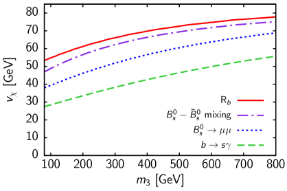
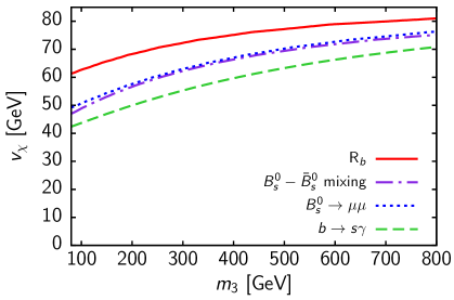
In what follows we use this correspondence to consider the constraints on the GM model from , – mixing, , and . These observables each put an upper bound on (equivalently ) as a function of . In each case we combine the experimental and GM theoretical uncertainties in quadrature and constrain the GM model prediction for the observable in question to lie within 2 of the experimental central value. We will refer to these as “tight” constraints.
However, in the GM model the contributions to , , and worsen the agreement with experiment compared to the SM limit (i.e., compared to taking or ). As we will see, the SM limit is already 0.8, 1.0, and 1.3 away from the experimental central values of these three observables, respectively. For this reason, we also consider a second, more conservative approach to constraining the parameter space for these three observables: we require that the GM model prediction lie within 2 of the best-fit value obtainable in the GM model (i.e., the SM limit), again combining the experimental and GM theoretical uncertainties in quadrature. We will refer to these more conservative constraints as “loose” constraints.
These “loose” and “tight” constraints are respectively shown in the right- and left-hand panels of Fig. 1.777With the exception of , we choose the input parameters for all our numerical results from the 2014 Review of Particle Physics Agashe:2014kda . For , we use the first combination of Tevatron and LHC measurements of the top quark mass ATLAS:2014wva . In particular, we set , , , , , and . In addition, we obtain the dependent parameters and at tree level. We thus edit the input files of SuperIso v3.3 which by default uses inputs from the 2011 Review of Particle Physics Nakamura:2010zzi . Details on each process follow.
IV.1
The -pole observable , defined as
| (29) |
has been calculated in the SM including two-loop electroweak Freitas:2012sy and three-loop QCD corrections. The correction to due to one-loop diagrams involving additional Higgs bosons has been calculated in the 2HDM Denner:1991ie ; Grant:1994ak . In the Type-I 2HDM, the contribution of the neutral scalars can be neglected Grant:1994ak as it is suppressed by a relative factor of compared to the charged Higgs contribution. The results for the Type-I 2HDM can easily be adapted to the GM model Haber:1999zh ; Chiang:2012cn .
Following Ref. Haber:1999zh , the one-loop charged Higgs correction to can be written as888The coefficient depends on the couplings and the bottom quark mass. Updated values of these quantities have a very small effect on the coefficient. For example, using more recent values from Ref. Haisch:2011up the change in the coefficient is 0.1%.
| (30) | |||||
where , , and we neglect in the loop calculation.999Full expressions including the dependence have been given in Refs. Haber:1999zh ; Chiang:2012cn . Because the constraint from is weaker than the other constraints, we use here only the approximation given in Eq. (30). Here is the running mass and is evaluated at . The approximation in Eq. (30) can be made because is suppressed by a factor of compared to Haber:1999zh ; Chiang:2012cn . The correction is always negative and interferes destructively with the SM contribution.
The measured value of is Baak:2014ora
| (31) |
while the SM prediction is Baak:2014ora . Therefore the 2 upper bound relative to the experimental central value yields the “tight” constraint , where we have combined the experimental and SM theoretical uncertainties in quadrature.101010Because the coefficients in Eq. (30) depend on the SM prediction in a complex way, the observable cannot straightforwardly be calculated using a ratio of the SM and GM constributions (as we will do with the other observables). For this reason, in the case only we take the theory uncertainty on the GM prediction to be the same as that of the SM prediction.
The SM prediction is 0.8 below the measured value; as the GM correction interferes destructively with the SM contribution, it increases the discrepancy between theory and experiment. As a result, the best agreement with the experimental measurement of in the GM model occurs in the SM limit (, ). Requiring that the GM prediction for lie within 2 of the SM value yields a “loose” constraint of .
As we see in Fig. 1, provides the weakest non-oblique “tight” and “loose” constraints. Furthermore, substantial improvement in the experimental measurement is unlikely in the near future, as this would require better Z-pole measurements using a next-generation collider like the International Linear Collider (ILC) with the GigaZ option Baer:2013cma .
IV.2 – mixing
The effect of charged scalars on – mixing in a Type-I 2HDM has been studied Athanasiu:1985ie by adapting results of similar processes on – mixing Abbott:1979dt . These can be extended to the – system, which is more constraining than the – system due to lower errors in both the experimental measurement and the SM prediction Lenz:2012mb . To leading order, the oscillation frequency of a meson in the GM model is determined by the mass splitting WahabElKaffas:2007xd
| (32) |
Here is a scaling factor, is the weak decay constant, is the bag parameter, is the meson mass, and111111The NLO QCD corrections to the charged Higgs contributions are known Urban:1997gw , but we do not include them here.
| (33) |
Here , , and . We set the top mass renormalization scale , where is the top quark pole mass. The Inami-Lim functions Inami:1980fz , , and are given by Mahmoudi:2009zx
| (34) |
Under the assumption that the overall coefficients do not vary substantially due to new scalar contributions, a prediction for in the GM model may be obtained using the ratio
| (35) |
Since , and are all positive, the GM model contribution interferes constructively with the SM contribution. Because the theoretical uncertainty on the mass splitting is due almost entirely to uncertainties in the coefficients of in Eq. (32), we scale the SM theoretical uncertainty by to obtain the theoretical uncertainty in the GM model, i.e., .
The measured value for the – mass difference is given by PDG
| (36) |
The largest uncertainty in the SM prediction comes from the lattice QCD calculation of . Using a CKMfitter Lenz:2012az ; CKMfitter average of several lattice results based on separate extractions of and , Ref. Nierste:2012qp obtains the SM prediction . However, a preliminary lattice calculation of the product from the Fermilab/MILC collaboration Bouchard:2011xj yields a larger uncertainty and considerably different central value, leading to Nierste:2012qp . For our numerical results we use the CKMfitter central value but take the more conservative uncertainty as advocated in Ref. Lenz:2011ti ,
| (37) |
The above results can be translated into an experimental measurement of and combined experimental and SM theoretical uncertainty of
| (38) |
The SM prediction is thus only 0.13 below the measured value.
In the case of – mixing, the charged Higgs contributions in the GM model increase the predicted value of , so that the best-fit value and the experimental central value are the same. Thus our “tight” and “loose” constraints from this observable are the same. The 2 constraint is , where we have combined the experimental and GM theoretical uncertainties in quadrature. The resulting constraint on the – plane is shown in the left and right panels of Fig. 1. It is slightly more constraining than the bounds from , and is about the same as the “loose” bound from .121212If we were to use the less-conservative prediction of , the uncertainty on becomes and the bound would tighten to match the “tight” bound from in the left-hand panel. If we were instead to use the central value , the best-fit reference point would become the SM prediction, , and the “loose” and “tight” bounds would each be slightly stronger than the corresponding bounds from . This variability illustrates the very large remaining theoretical uncertainty in this observable. In both cases the bound is weaker than that from . An improvement in the constraint from – mixing relies on an improved lattice determination of .
IV.3
A full leading-order computation of the average time-integrated branching ratio in the Aligned 2HDM Pich:2009sp was recently performed in Ref. Li:2014fea . The calculation can be easily specialized to the Type-I 2HDM and hence to the GM model; the result is conveniently expressed in terms of a ratio to the SM prediction,
| (39) |
where the Wilson coefficients and are given by Li:2014fea
| (40) |
with and as before.131313Note that for , the expression in square brackets can be expanded in powers of and reads (41) Here is the top quark pole mass and is the running mass. The theoretical uncertainty on the resulting GM branching ratio is taken to be .
The approximation made in Eq. (39) is to neglect contributions from the Wilson coefficients and , which arise from scalar and pseudoscalar penguins and box diagrams and are suppressed by an extra factor of compared to . The expression for includes next-to-leading order (NLO) electroweak and QED corrections, as well as NLO and next-to-next-to-leading order (NNLO) QCD corrections. We note that the expression for the contribution to has the same dependence on and as the expression for the correction to in the limit given in Eq. (30). This is because the charged Higgs contribution to comes from the same penguin diagrams as in , but with a generation-changing vertex in place of the generation-conserving vertex and .
The current experimental measurement of from a combination of CMS and LHCb results is CMSandLHCbCollaborations:2013pla
| (42) |
The SM prediction is given in Ref. Li:2014fea as
| (43) |
This number differs slightly from the result in Ref. Bobeth:2013uxa , upon which it is based, due to the use of a slightly different central value and more conservative uncertainty on the top quark mass. These yield an experimental measurement of and combined experimental and SM theoretical uncertainty of
| (44) |
In particular, the SM prediction, , is 1.0 above the current experimental value.
The 2 constraint on the GM model relative to the experimental central value yields a bound of , where we have combined the experimental and GM model theoretical uncertainties in quadrature. This “tight” constraint is shown in the left-hand panel of Fig. 1; it is stronger than the corresponding constraints from and – mixing, as previously discussed, but remains weaker than the “tight” constraint.
However, the GM model contribution to in Eq. (40) is always negative, leading to constructive interference with the SM contribution and increasing the prediction for compared to its value in the SM. As the SM value is already larger than the experimental value (), the best agreement with the experimental measurement of in the GM model occurs in the limit or (i.e., the SM limit). The best-fit 2 bound taken relative to the SM prediction yields a “loose” constraint of , which is shown in the right-hand panel of Fig. 1. The “loose” constraint from is also weaker than that from .
The current uncertainty on is dominated by the experimental statistical uncertainty. This has the potential to be significantly reduced in the near future as more data is collected at the LHC. In particular, the upgraded LHCb experiment is expected to measure with an ultimate experimental uncertainty of better than 10% with 50 fb-1 of data Bediaga:2012py , which corresponds to about ten years of LHC running. Assuming an experimental rate consistent with the SM prediction and no change in the theoretical uncertainty, this would correspond to a combined uncertainty on of 0.12. This measurement thus has the potential to become the most stringent constraint on the GM model parameter space in the near future.
IV.4
The branching ratio has been measured at several different experiments, including CLEO, BaBar, Belle, and ALEPH. The current experimental average from the Heavy Flavour Averaging Group is Asner:2010qj ; PDG 141414The most recent measurement from BaBar, which has not yet been incorporated into this average, reads Lees:2012ufa .
| (45) |
for a photon energy GeV.
is known up to NNLO in QCD in the SM Misiak:2006zs ; Becher:2006pu .151515This calculation is an estimate insofar as charm-mass-dependent contributions have been incorporated using an interpolation in , resulting in a contribution to the theory uncertainty from the interpolation ambiguity. The two current SM predictions are Misiak:2006zs and Becher:2006pu . These predictions differ due to different approaches to handling higher-order contributions to the photon energy cutoff corrections; however, their difference is within the theoretical uncertainty due to uncalculated higher orders Misiak:2006zs .
The charged Higgs contributions in the Type-I 2HDM, first calculated in Ref. Barger:1989fj , are themselves now known up to NLO in QCD Ciuchini:1997xe . Because will provide the most stringent constraint on the GM model parameter space, we will use the full implementation of the SM and 2HDM contributions in the public code SuperIso v3.3 SuperIso , which is based on the calculations in Refs. Misiak:2006zs ; Misiak:2006ab . SuperIso calls the code 2HDMC v1.6.4 2HDMC for spectrum calculations within the Type-I 2HDM.
In the limit or , the calculation of by SuperIso v3.3, using the input parameters given in footnote 7, yields a prediction
| (46) |
The difference compared to the SM predictions quoted above is primarily due to differences in the input parameters, particularly and Nazila . However, the difference is still within the theoretical uncertainty due to parametric uncertainties of Misiak:2006zs . We take the total theoretical uncertainty on this SM prediction to be from Ref. Misiak:2006zs . Combining this in quadrature with the experimental uncertainty yields a total uncertainty of . In particular, the value of in the SM limit is 1.3 below the experimental value.
The charged Higgs contribution to in the GM model interferes destructively with the SM contribution, leading to a smaller predicted value for than in the SM. Because the SM prediction is already below the experimental central value, the best agreement with the experimental measurement in the GM model occurs in the limit or (i.e., the SM limit). Since even the SM limit yields a prediction that is only 0.7 from the experimental bound, the 2 experimental constraint on the GM – plane is quite strong, as can be seen in the left panel of Fig. 1. This bound corresponds to (“tight” constraint), where we have combined the experimental and GM theoretical uncertainties in quadrature; again, here we estimate the GM theory uncertainty to be that of the SM prediction scaled by a ratio of the GM and SM predictions. In comparison, the constraint with respect to the best-fit point, the SM limit, yields (“loose” constraint). This is shown in the right panel of Fig. 1 together with the “loose” constraints from the other observables. In either case, is the strongest constraint on these parameters.
Because of the large theoretical uncertainty on and the sensitivity of the resulting constraint to the particular choice of input parameters and the handling of partial higher-order corrections, we consider it safer to take the more conservative approach and apply the “loose” constraint from as our primary constraint on the – plane. We will nevertheless also show the effect of applying the “tight” constraint in our numerical scans.
The current theoretical and experimental uncertainties on are comparable in size. The experimental uncertainty is expected to be reduced with measurements at the super factory experiment Belle II currently under construction at KEK. A conservative treatment of systematics yields an estimated future experimental precision on of 7% (i.e., about ) with 5 ab-1 of data, or 6% (i.e., about ) with 50 ab-1 of data Aushev:2010bq . With the current theoretical uncertainties, these would reduce the combined uncertainty only to about or , respectively. A more significant improvement in the constraining power of would require a simultaneous reduction in the theoretical uncertainty.
V Numerical results
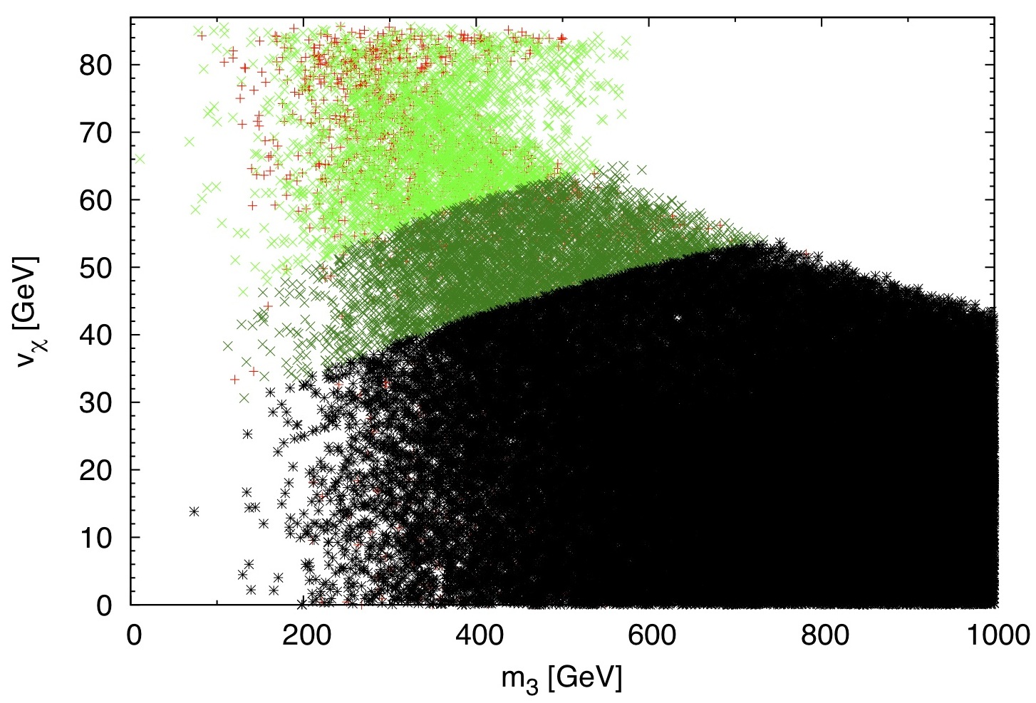
We now illustrate the effects of the indirect experimental constraints from (computed using SuperIso v3.3 SuperIso , which calls 2HDMC v1.6.4 2HDMC ) and the parameter on the parameter space of the GM model. We scan over the full range of GM model parameters allowed after imposing the theoretical requirements of perturbative unitarity, bounded-from-belowness of the potential, and the absence of alternative custodial-symmetry–breaking minima HKL . We require that either or has mass 125 GeV and set the SM Higgs vev using . We take , which fully populates the mass ranges shown in Figs. 2–6 below. In Fig. 6 we will include additional points generated by a dedicated scan with in order to better populate the low-mass region. In all cases, we show the effects of the following constraints:
-
•
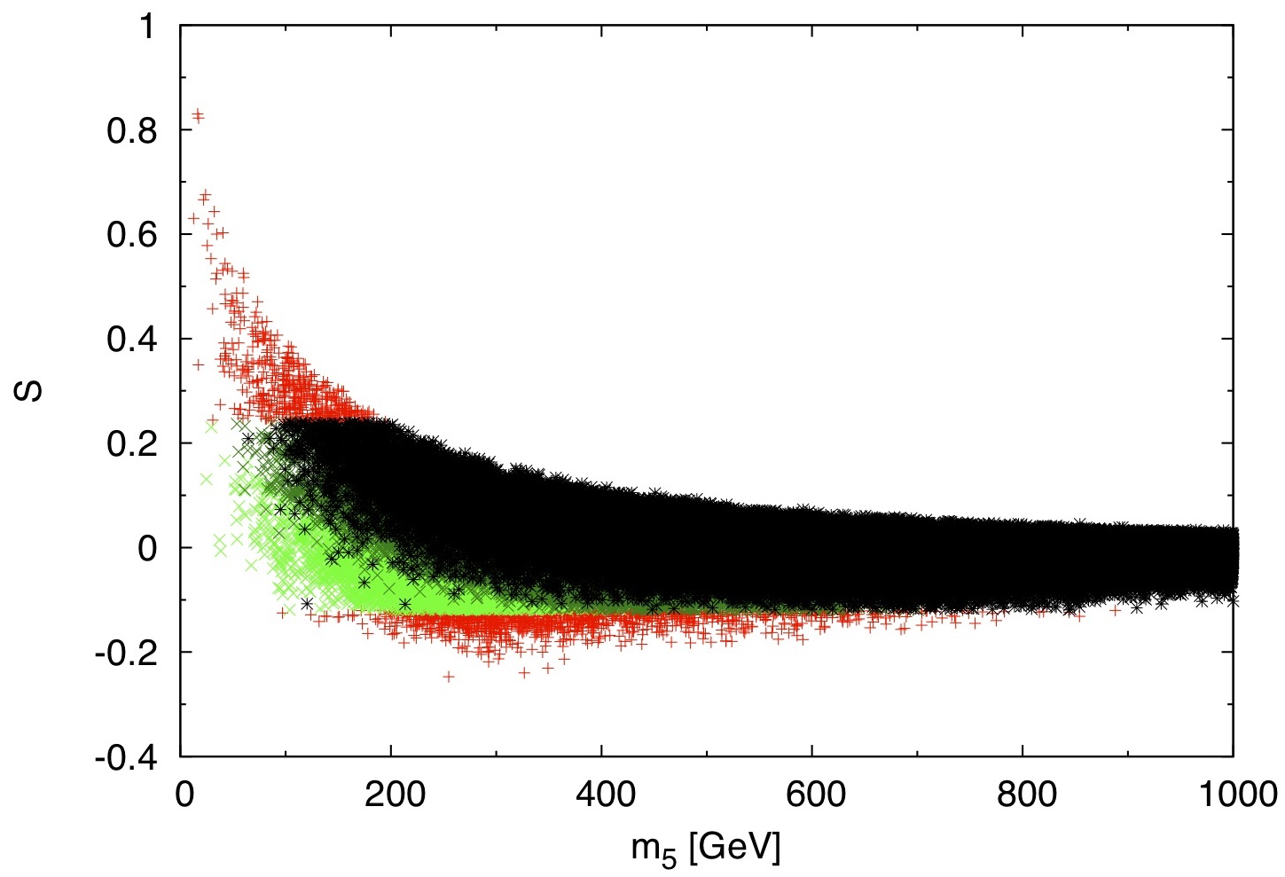
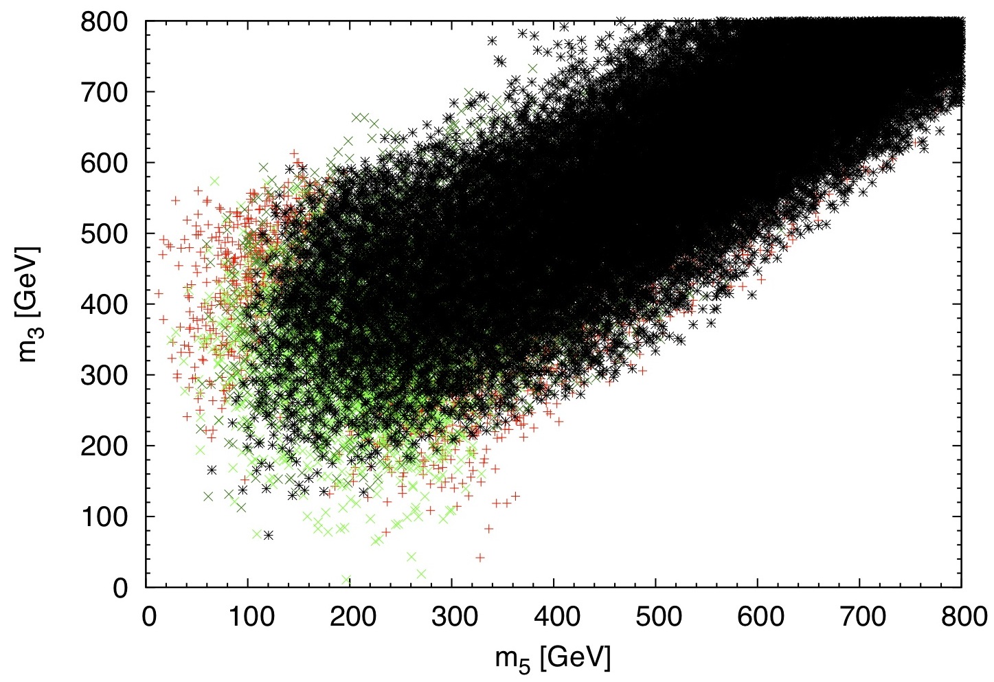
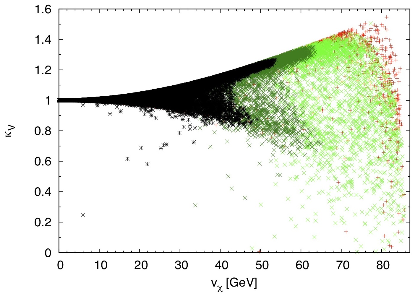
The prediction for yields after marginalizing over the parameter. Points eliminated by this constraint are shown by red (medium gray) shapes.
-
•
The prediction for lies within of the model point that gives the best agreement with the experimental measurement (“loose” constraint). We combine theoretical and experimental uncertainties in quadrature. Points eliminated by this constraint are shown by light green (light gray) shapes.
-
•
The prediction for lies within of the experimental measurement (“tight” constraint). We combine theoretical and experimental uncertainties in quadrature. Points eliminated by this constraint are shown by dark green (dark gray) shapes.
Points depicted in black are allowed by all constraints.
We start by showing the effect of the measurement on the – plane in the left panel of Fig. 2. The prediction for in the GM model depends only on these two parameters. We see that, due to its interplay with the decoupling effect of falling with increasing triplet masses HKL , the “loose” constraint eliminates all model points with GeV and the “tight” constraint eliminates all model points with GeV.161616This constraint is considerably more stringent than the upper bound on obtained in the spirit of Ref. Barger:1989fj by requiring to avoid parameter regions in which the top quark Yukawa coupling becomes too large ( plays the same role as is played by in the Type-I 2HDM); this requirement yields GeV.
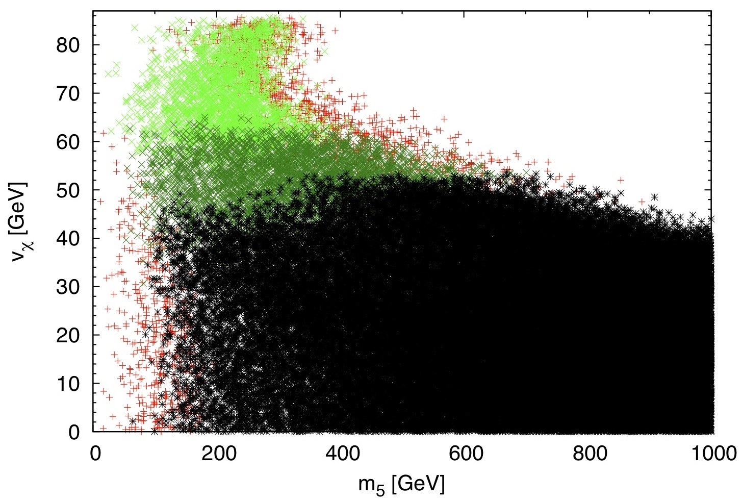
This is reflected in the right panel of Fig. 2, where we plot as a function of . Because in general, values of up to the limit of GeV are allowed even for masses as low as 100 GeV under the “loose” constraint.
This indirect constraint on as a function of is especially interesting in light of the recent recasting Chiang:2014bia of an ATLAS measurement ATLAS-CONF-2014-013 of the like-sign cross section in 8 TeV data in the context of the GM model. The like-sign cross section receives contributions especially from the -channel production of in fusion, followed by decays back to . The analysis of Ref. Chiang:2014bia excludes a triangular region of parameter space in the – plane extending from GeV to 610 GeV at GeV, down to GeV at GeV.
In the right panel of Fig. 2 we also see the effect of the parameter constraint, which eliminates a few model points at very low , as well as moderate to high and high . This is illustrated in more detail in Fig. 3. In particular, points with very low values of tend to have a large – splitting, which leads to large positive values of the parameter.
Finally we show the effect of the constraints from and the parameter on the allowed ranges of the couplings of the 125 GeV Higgs boson to and boson pairs and to fermion pairs. We parameterize these couplings in terms of scaling factors and LHCHiggsCrossSectionWorkingGroup:2012nn , which represent the () and couplings, respectively, normalized to their SM values. In the GM model, these couplings are given in terms of the triplet vev and the custodial singlet mixing angle by
| (47) |
where corresponds to the SM Higgs vev.171717For a small number of points in our scan, the 125 GeV Higgs boson is , and the lighter custodial singlet has a mass below 125 GeV. In these cases, we plot the coupling scaling factors and that represent the () and couplings, respectively, normalized to their SM values. These couplings are given in this case by (48)
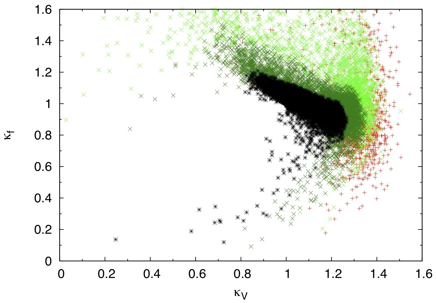
One of the most interesting features of the GM model is the possibility that , which is not possible at tree level in extended Higgs sectors that contain only SU(2)L doublets and/or singlets. In particular, for maximal and (corresponding to being entirely composed of triplet), can be as large as 1.6. This maximal value is reduced to by the upper bound on imposed by the “loose” constraint, as shown in the left panel of Fig. 4. It would be reduced even further to by the “tight” constraint.
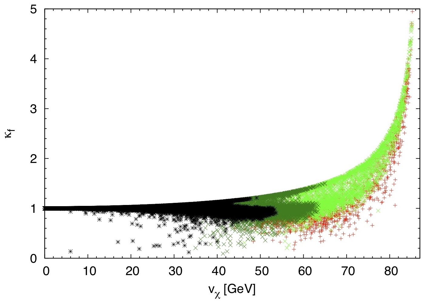
Similarly, can be significantly enhanced in the GM model if is small. By limiting the maximum size of , the “loose” constraint puts a lower bound on , and thereby imposes an upper bound on of , as shown in the right panel of Fig. 4. The “tight” constraint on would reduce this further to .
The parameter measurement does not further constrain the allowed ranges of either or in a significant way once either of the constraints has been applied.
Finally we show the allowed range of correlations between and in Fig. 5. We note in particular that the GM model can accommodate simultaneous enhancements of both and . Such enhancements are constrained by the measurement to lie below (“loose” constraint). The “tight” constraint would reduce this to about 1.09. This is interesting primarily because Higgs coupling fits from LHC data suffer from a flat direction Zeppenfeld:2000td if unobserved decay modes are allowed, corresponding to a simultaneous increase in the unobserved decay branching ratio and in all the Higgs couplings to SM particles. This flat direction can be cut off by imposing additional theory assumptions, such as the absence of new, unobserved Higgs decay modes Zeppenfeld:2000td or the imposition of valid when the Higgs sector contains only isospin doublets and/or singlets Duhrssen:2004cv . The GM model provides a concrete example of a model that violates the second assumption while being consistent with other experimental constraints. The flat direction could also be tamed by constraining the total Higgs width through measurements of off-shell Caola:2013yja ; CMS:2014ala ; the interpretation of this measurement in terms of a Higgs width constraint, however, is itself model-dependent Englert:2014aca and it is not yet clear what effect the presence of additional Higgs states will have.
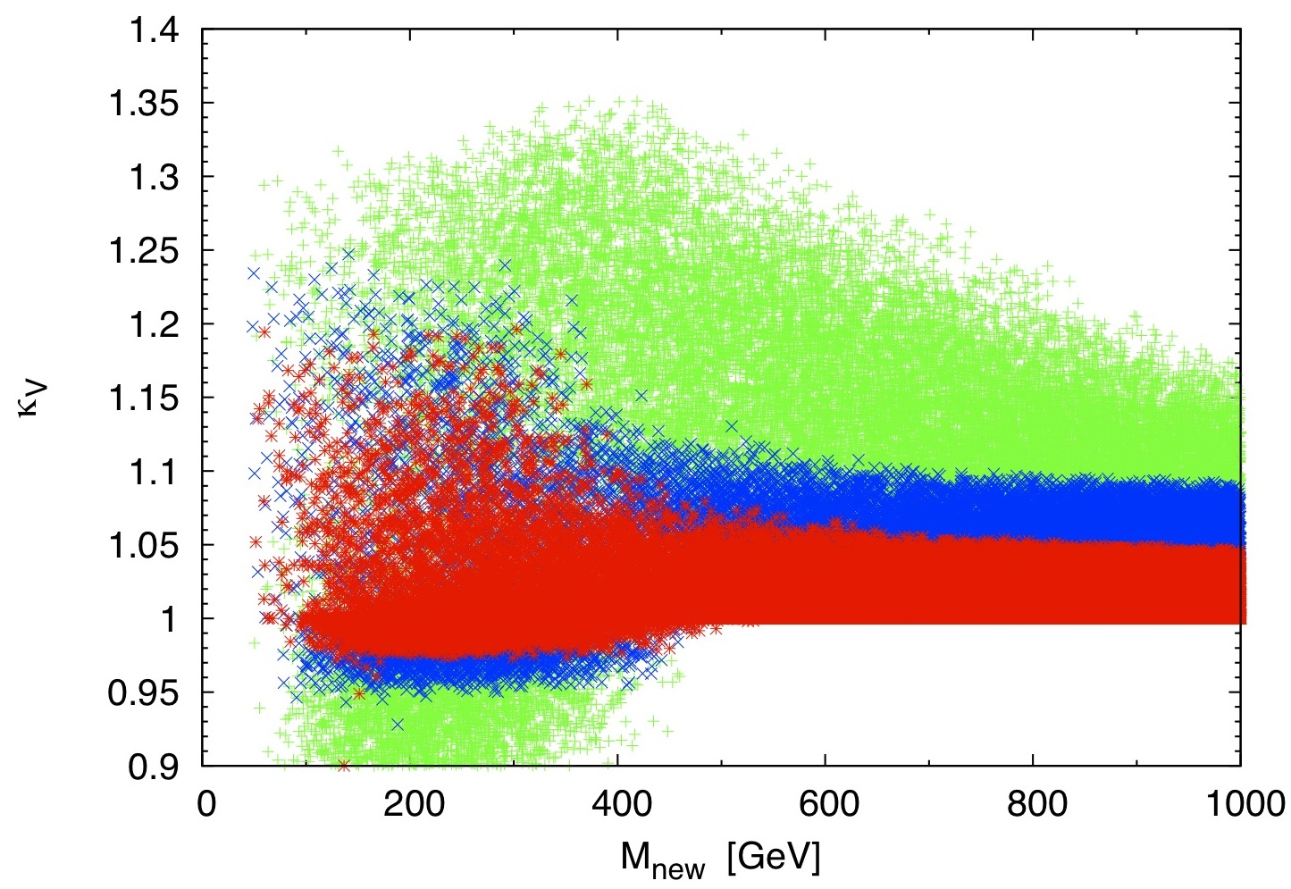
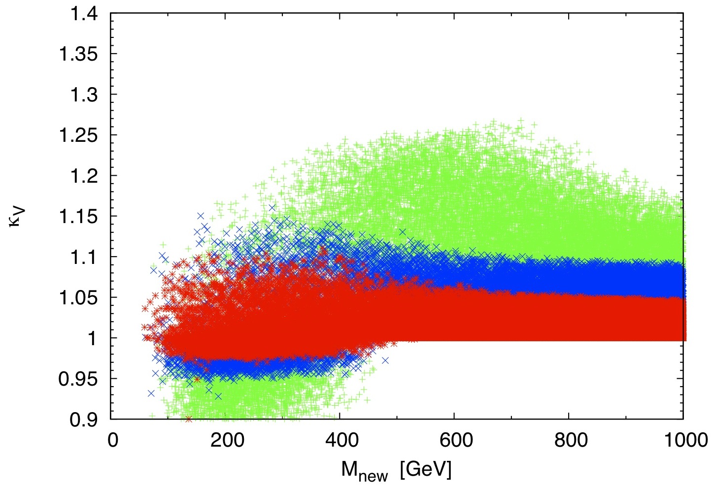
Crucially, however, the simultaneous enhancement of and occurs only when the new scalars are relatively light. This is illustrated in Fig. 6, where we plot as a function of the mass of the lightest new scalar, for within 5% (red) or 10% (blue) of . The remaining points are shown in green. Under the “loose” constraint, for within 5% of , an 18% enhancement of these couplings is possible only when at least one of the new scalars has mass below about 375 GeV. This provides a complementary (albeit model dependent) way to constrain the flat direction by directly searching for the new scalars. We leave a full consideration of the direct-search constraints on these additional scalars to future work.
VI Conclusions
In this paper we updated the indirect experimental constraints on the GM model coming from electroweak and -physics observables—in particular the parameter, , , – mixing, and . Except for the parameter, all of these constrain only two of the GM model parameters: the isospin-triplet vev and the custodial-triplet mass . We gave the analytic expressions for the one-loop contributions from the additional Higgs bosons for the parameter, , – mixing, and ; in the case of the parameter and these are in the approximation that the new scalars are heavy compared to . For we adapted the 2HDM calculation implemented in the code SuperIso. The constraints from , – mixing, and have not been studied in the GM model before.
We found that is currently the strongest of the -physics constraints on the GM model. However, this may be surpassed in the next few years by the constraint from , which will become more important as its statistical uncertainty is reduced with further LHC data-taking. Combined with the theoretical requirements of vacuum stability and perturbativity, the constraint puts a conservative upper bound of about 65 GeV on the isospin-triplet vev , which leads to upper bounds on the , , and couplings. In particular, a simultaneous enhancement of the , , and couplings of up to 18% compared to their SM values is still allowed by the indirect constraints, leading to a simultaneous enhancement of all the Higgs production cross sections by up to 39%. Such an enhancement could mask (and be masked by) the presence of undetected new decay modes of the SM-like Higgs boson at the LHC.
Acknowledgements.
We thank F. Mahmoudi for helpful discussions about SuperIso. H.E.L. also thanks the organizers of the Lisbon Workshop on Multi-Higgs Models 2014 for partial support and a stimulating environment while part of this work was performed. This work was supported by the Natural Sciences and Engineering Research Council of Canada. K.H. was also supported by the Government of Ontario through an Ontario Graduate Scholarship.References
- (1) G. Aad et al. [ATLAS Collaboration], Phys. Lett. B 716, 1 (2012) [arXiv:1207.7214 [hep-ex]]; S. Chatrchyan et al. [CMS Collaboration], Phys. Lett. B 716, 30 (2012) [arXiv:1207.7235 [hep-ex]].
- (2) H. Georgi and M. Machacek, Nucl. Phys. B 262, 463 (1985).
- (3) M. S. Chanowitz and M. Golden, Phys. Lett. B 165, 105 (1985).
- (4) J. F. Gunion, R. Vega and J. Wudka, Phys. Rev. D 42, 1673 (1990).
- (5) J. F. Gunion, R. Vega and J. Wudka, Phys. Rev. D 43, 2322 (1991).
- (6) J. F. Gunion, H. E. Haber, G. L. Kane, and S. Dawson, The Higgs Hunter’s Guide (Westview, Boulder, Colorado, 2000).
- (7) H. E. Haber and H. E. Logan, Phys. Rev. D 62, 015011 (2000) [hep-ph/9909335].
- (8) M. Aoki and S. Kanemura, Phys. Rev. D 77, 095009 (2008) [arXiv:0712.4053 [hep-ph]]; erratum Phys. Rev. D 89, 059902 (2014).
- (9) S. Godfrey and K. Moats, Phys. Rev. D 81, 075026 (2010) [arXiv:1003.3033 [hep-ph]].
- (10) I. Low and J. Lykken, JHEP 1010, 053 (2010) [arXiv:1005.0872 [hep-ph]]; I. Low, J. Lykken and G. Shaughnessy, Phys. Rev. D 86, 093012 (2012) [arXiv:1207.1093 [hep-ph]].
- (11) H. E. Logan and M.-A. Roy, Phys. Rev. D 82, 115011 (2010) [arXiv:1008.4869 [hep-ph]].
- (12) A. Falkowski, S. Rychkov and A. Urbano, JHEP 1204, 073 (2012) [arXiv:1202.1532 [hep-ph]].
- (13) S. Chang, C. A. Newby, N. Raj and C. Wanotayaroj, Phys. Rev. D 86, 095015 (2012) [arXiv:1207.0493 [hep-ph]].
- (14) D. Carmi, A. Falkowski, E. Kuflik, T. Volansky and J. Zupan, JHEP 1210, 196 (2012) [arXiv:1207.1718 [hep-ph]].
- (15) C.-W. Chiang and K. Yagyu, JHEP 1301, 026 (2013) [arXiv:1211.2658 [hep-ph]].
- (16) C.-W. Chiang, A.-L. Kuo and K. Yagyu, JHEP 1310, 072 (2013) [arXiv:1307.7526 [hep-ph]].
- (17) S. Kanemura, M. Kikuchi and K. Yagyu, Phys. Rev. D 88, 015020 (2013) [arXiv:1301.7303 [hep-ph]].
- (18) C. Englert, E. Re and M. Spannowsky, Phys. Rev. D 87, 095014 (2013) [arXiv:1302.6505 [hep-ph]].
- (19) R. Killick, K. Kumar and H. E. Logan, Phys. Rev. D 88, 033015 (2013) [arXiv:1305.7236 [hep-ph]].
- (20) G. Belanger, B. Dumont, U. Ellwanger, J. F. Gunion and S. Kraml, Phys. Rev. D 88, 075008 (2013) [arXiv:1306.2941 [hep-ph]].
- (21) C. Englert, E. Re and M. Spannowsky, Phys. Rev. D 88, 035024 (2013) [arXiv:1306.6228 [hep-ph]].
- (22) A. Efrati and Y. Nir, arXiv:1401.0935 [hep-ph].
- (23) K. Hartling, K. Kumar and H. E. Logan, Phys. Rev. D 90, 015007 (2014) [arXiv:1404.2640 [hep-ph]].
- (24) C.-W. Chiang and T. Yamada, arXiv:1404.5182 [hep-ph].
- (25) C.-W. Chiang, S. Kanemura and K. Yagyu, arXiv:1407.5053 [hep-ph].
- (26) S. I. Godunov, M. I. Vysotsky and E. V. Zhemchugov, arXiv:1408.0184 [hep-ph].
- (27) S. Chang and J. G. Wacker, Phys. Rev. D 69, 035002 (2004) [hep-ph/0303001].
- (28) S. Chang, JHEP 0312, 057 (2003) [hep-ph/0306034].
- (29) L. Cort, M. Garcia and M. Quiros, Phys. Rev. D 88, 075010 (2013) [arXiv:1308.4025 [hep-ph]].
- (30) M. Garcia-Pepin, S. Gori, M. Quiros, R. Vega, R. Vega-Morales and T. T. Yu, arXiv:1409.5737 [hep-ph].
- (31) S. El Hedri, P. J. Fox and J. G. Wacker, arXiv:1311.6488 [hep-ph].
- (32) P. Galison, Nucl. Phys. B 232, 26 (1984).
- (33) R. W. Robinett, Phys. Rev. D 32, 1780 (1985).
- (34) H. E. Logan, hep-ph/9906332.
- (35) J. Hisano and K. Tsumura, Phys. Rev. D 87, 053004 (2013) [arXiv:1301.6455 [hep-ph]].
- (36) C. Alvarado, L. Lehman and B. Ostdiek, JHEP 1405, 150 (2014) [arXiv:1404.3208 [hep-ph]].
- (37) For a recent review, see G. C. Branco, P. M. Ferreira, L. Lavoura, M. N. Rebelo, M. Sher and J. P. Silva, Phys. Rept. 516, 1 (2012) [arXiv:1106.0034 [hep-ph]].
- (38) F. Mahmoudi, Comput. Phys. Commun. 178, 745 (2008) [arXiv:0710.2067 [hep-ph]]; Comput. Phys. Commun. 180, 1579 (2009) [arXiv:0808.3144 [hep-ph]]; Comput. Phys. Commun. 180, 1718 (2009).
- (39) X.-Q. Li, J. Lu and A. Pich, arXiv:1404.5865 [hep-ph].
- (40) A. Pich and P. Tuzon, Phys. Rev. D 80, 091702 (2009) [arXiv:0908.1554 [hep-ph]].
- (41) H. Baer, T. Barklow, K. Fujii, Y. Gao, A. Hoang, S. Kanemura, J. List and H. E. Logan et al., arXiv:1306.6352 [hep-ph].
- (42) M. E. Peskin and T. Takeuchi, Phys. Rev. D 46, 381 (1992).
- (43) M. Baak, J. Cuth, J. Haller, A. Hoecker, R. Kogler, K. Moenig, M. Schott and J. Stelzer, arXiv:1407.3792 [hep-ph].
- (44) K. A. Olive et al. [Particle Data Group Collaboration], Chin. Phys. C 38, 090001 (2014).
- (45) ATLAS, CDF, CMS, and D0 Collaborations, arXiv:1403.4427 [hep-ex].
- (46) K. Nakamura et al. [Particle Data Group Collaboration], J. Phys. G 37, 075021 (2010).
- (47) A. Freitas and Y.-C. Huang, JHEP 1208, 050 (2012) [Erratum-ibid. 1305, 074 (2013)] [Erratum-ibid. 1310, 044 (2013)] [arXiv:1205.0299 [hep-ph]].
- (48) A. Denner, R. J. Guth, W. Hollik and J. H. Kuhn, Z. Phys. C 51, 695 (1991).
- (49) A. K. Grant, Phys. Rev. D 51, 207 (1995) [hep-ph/9410267].
- (50) U. Haisch and S. Westhoff, JHEP 1108, 088 (2011) [arXiv:1106.0529 [hep-ph]].
- (51) G. G. Athanasiu, P. J. Franzini and F. J. Gilman, Phys. Rev. D 32, 3010 (1985).
- (52) L. F. Abbott, P. Sikivie and M. B. Wise, Phys. Rev. D 21, 1393 (1980).
- (53) A. Lenz, arXiv:1205.1444 [hep-ph].
- (54) A. Wahab El Kaffas, P. Osland and O. M. Ogreid, Phys. Rev. D 76, 095001 (2007) [arXiv:0706.2997 [hep-ph]].
- (55) J. Urban, F. Krauss, U. Jentschura and G. Soff, Nucl. Phys. B 523, 40 (1998) [hep-ph/9710245].
- (56) T. Inami and C. S. Lim, Prog. Theor. Phys. 65, 297 (1981) [Erratum-ibid. 65, 1772 (1981)].
- (57) F. Mahmoudi and O. Stal, Phys. Rev. D 81, 035016 (2010) [arXiv:0907.1791 [hep-ph]].
- (58) J. Beringer et al. [Particle Data Group Collaboration], Phys. Rev. D 86, 010001 (2012).
- (59) A. Lenz, U. Nierste, J. Charles, S. Descotes-Genon, H. Lacker, S. Monteil, V. Niess and S. T’Jampens, Phys. Rev. D 86, 033008 (2012) [arXiv:1203.0238 [hep-ph]].
- (60) CKMfitter results are summarized at http://ckmfitter.in2p3.fr. The Rfit method used by CKMfitter is described in J. Charles et al. [CKMfitter Group Collaboration], Eur. Phys. J. C 41, 1 (2005) [hep-ph/0406184].
- (61) U. Nierste, arXiv:1212.5805 [hep-ph].
- (62) C. M. Bouchard, E. D. Freeland, C. Bernard, A. X. El-Khadra, E. Gamiz, A. S. Kronfeld, J. Laiho and R. S. Van de Water, PoS LATTICE 2011, 274 (2011) [arXiv:1112.5642 [hep-lat]].
- (63) A. Lenz and U. Nierste, arXiv:1102.4274 [hep-ph].
- (64) CMS and LHCb Collaborations [CMS and LHCb Collaboration], CMS-PAS-BPH-13-007.
- (65) C. Bobeth, M. Gorbahn, T. Hermann, M. Misiak, E. Stamou and M. Steinhauser, Phys. Rev. Lett. 112, 101801 (2014) [arXiv:1311.0903 [hep-ph]].
- (66) R. Aaij et al. [LHCb Collaboration], Eur. Phys. J. C 73, 2373 (2013) [arXiv:1208.3355 [hep-ex]].
- (67) D. Asner et al. [Heavy Flavor Averaging Group Collaboration], arXiv:1010.1589 [hep-ex].
- (68) J. P. Lees et al. [BaBar Collaboration], Phys. Rev. D 86, 112008 (2012) [arXiv:1207.5772 [hep-ex]].
- (69) M. Misiak, H. M. Asatrian, K. Bieri, M. Czakon, A. Czarnecki, T. Ewerth, A. Ferroglia and P. Gambino et al., Phys. Rev. Lett. 98, 022002 (2007) [hep-ph/0609232].
- (70) T. Becher and M. Neubert, Phys. Rev. Lett. 98, 022003 (2007) [hep-ph/0610067].
- (71) V. D. Barger, J. L. Hewett and R. J. N. Phillips, Phys. Rev. D 41, 3421 (1990).
- (72) M. Ciuchini, G. Degrassi, P. Gambino and G. F. Giudice, Nucl. Phys. B 527, 21 (1998) [hep-ph/9710335].
- (73) M. Misiak and M. Steinhauser, Nucl. Phys. B 764, 62 (2007) [hep-ph/0609241].
- (74) D. Eriksson, J. Rathsman and O. Stal, Comput. Phys. Commun. 181, 189 (2010) [arXiv:0902.0851 [hep-ph]]; Comput. Phys. Commun. 181, 833 (2010).
- (75) F. Mahmoudi, private communication.
- (76) T. Aushev, W. Bartel, A. Bondar, J. Brodzicka, T. E. Browder, P. Chang, Y. Chao and K. F. Chen et al., arXiv:1002.5012 [hep-ex].
-
(77)
ATLAS Collaboration,
ATLAS-CONF-2014-013,
available from
http://cds.cern.ch. - (78) A. David et al. [LHC Higgs Cross Section Working Group Collaboration], arXiv:1209.0040 [hep-ph].
- (79) D. Zeppenfeld, R. Kinnunen, A. Nikitenko and E. Richter-Was, Phys. Rev. D 62, 013009 (2000) [hep-ph/0002036]; A. Djouadi, R. Kinnunen, E. Richter-Was, H. U. Martyn, K. A. Assamagan, C. Balazs, G. Belanger and E. Boos et al., hep-ph/0002258.
- (80) M. Duhrssen, S. Heinemeyer, H. Logan, D. Rainwater, G. Weiglein and D. Zeppenfeld, Phys. Rev. D 70, 113009 (2004) [hep-ph/0406323]; K. A. Assamagan et al. [Higgs Working Group Collaboration], hep-ph/0406152.
- (81) F. Caola and K. Melnikov, Phys. Rev. D 88, 054024 (2013) [arXiv:1307.4935 [hep-ph]].
- (82) CMS Collaboration, CMS-PAS-HIG-14-002; The ATLAS collaboration, ATLAS-CONF-2014-042; available from http://cds.cern.ch.
- (83) C. Englert and M. Spannowsky, arXiv:1405.0285 [hep-ph]; M. Ghezzi, G. Passarino and S. Uccirati, arXiv:1405.1925 [hep-ph]; G. Cacciapaglia, A. Deandrea, G. D. La Rochelle and J. B. Flament, arXiv:1406.1757 [hep-ph]; A. Azatov, C. Grojean, A. Paul and E. Salvioni, arXiv:1406.6338 [hep-ph].