Behavior of different numerical schemes for population genetic drift problems

Minxin Chen Center for System Biology and Department of Mathematics, Soochow University, Suzhou 215006, China (). chenmx@gmail.com    Chun Liu Department of Mathematics, Pennsylvania State University, University Park, PA, 16802, USA (). liu@psu.edu    Shixin Xu Corresponding author. Department of Mathematics, Soochow University, Suzhou 215006, China (). Department of Applied and Computational Mathematics and Statics, University of Notre Dame, Notre Dame, IN, 46556, USA. xsxztr@hotmail.com    Xingye Yue Department of Mathematics, Soochow University, Suzhou 215006, China (). xyyue@suda.edu.cn    Ran Zhang Department of Mathematics, Fudan University, Shanghai 200433, China () 12110180047@fudan.edu.cn
Abstract

In this paper, we focus on numerical methods for the genetic drift problems, which is governed by a degenerated convection-dominated parabolic equation. Due to the degeneration and convection, Dirac singularities will always be developed at boundary points as time evolves. In order to find a complete solution which should keep the conservation of total probability and expectation, three different schemes based on finite volume methods are used to solve the equation numerically: one is a upwind scheme, the other two are different central schemes. We observed that all the methods are stable and can keep the total probability, but have totally different long-time behaviors concerning with the conservation of expectation. We prove that any extra infinitesimal diffusion leads to a same artificial steady state. So upwind scheme does not work due to its intrinsic numerical viscosity. We find one of the central schemes introduces a numerical viscosity term too, which is beyond the common understanding in the convection-diffusion community. Careful analysis is presented to prove that the other central scheme does work. Our study shows that for this kind of problems, the numerical methods must be carefully chosen and any method with intrinsic numerical viscosity should be avoided.

keywords:
Genetic drift equation, complete solution, finite volume method, convection-diffusion, degenerate parabolic equation
AMS:
35K65 65M06 92D10
\slugger

mmsxxxxxxxx–x

1 Introduction

The number of a particular gene (allele) of one locus in the population varies randomly from generation to generation. This process is a kind of stochastic process and named as genetic drift, which was first introduced by one of the founders in the field of population genetics, S. Wright [24]. Genetic drift plays an important role in mutation, selection and molecular evolution [7, 16]. Mathematical descriptions of genetic drift are typically built upon the Wright-Fisher model [10, 25] or its diffusion limit [11, 12, 14]. The Wright-Fisher model describes the dynamics of a gene with two alleles, A or B in a population of fixed size, N. The model is formulated as a discrete-time Markov chain. If Xksubscript𝑋𝑘X_{k} denotes the number of A in kthsubscript𝑘𝑡k_{th} generation, then NXk𝑁subscript𝑋𝑘N-X_{k} is the number of B𝐵B and the transition probabilities are the following binomial distribution:

(1) P(Xn+1=j|Xn=i)=CNj(iN)j(1iN)Nj.𝑃subscript𝑋𝑛1conditional𝑗subscript𝑋𝑛𝑖superscriptsubscript𝐶𝑁𝑗superscript𝑖𝑁𝑗superscript1𝑖𝑁𝑁𝑗\displaystyle P(X_{n+1}=j|X_{n}=i)=C_{N}^{j}\left(\frac{i}{N}\right)^{j}\left(1-\frac{i}{N}\right)^{N-j}.

The first and second conditional moments of the Wright-Fisher process satisfy [8]

(2) E[Xk+1|Xk]=Xk,𝐸delimited-[]conditionalsubscript𝑋𝑘1subscript𝑋𝑘subscript𝑋𝑘\displaystyle E[X_{k+1}|X_{k}]=X_{k},
(3) Var[Xk+1|Xk]=Xk(1XkN).𝑉𝑎𝑟delimited-[]conditionalsubscript𝑋𝑘1subscript𝑋𝑘subscript𝑋𝑘1subscript𝑋𝑘𝑁\displaystyle Var[X_{k+1}|X_{k}]=X_{k}(1-\frac{X_{k}}{N}).

The first condition expresses the neutrality. A basic phenomenon of neutral Wright-Fisher model without mutation is that, either all copies of allele A are lost from the population or all the individuals carry allele A. This is the phenomenon of fixation. And the allele will fix with probability equal to its initial frequency. For a fixed population size, Wright-Fisher model works well, but if the size of the population changes over time, the diffusion approximation come to its own right. In [10] and [25], the diffusion approximation is first introduced to model the genetic drift, Moran [11] and Kimura [12] substantially extended and developed this approach. If we describe the process by x(t)𝑥𝑡x(t), the fraction of type A𝐴A genes at time t𝑡t, and f(x,t)𝑓𝑥𝑡f(x,t) denotes the probability density of x𝑥x at time t𝑡t, Kimura [12, 15, 26] showed that f(x,t)𝑓𝑥𝑡f(x,t) obeys the following diffusion equation,

f(x,t)t+j(x,t)x=0,𝑓𝑥𝑡𝑡𝑗𝑥𝑡𝑥0\frac{\partial f(x,t)}{\partial t}+\frac{\partial j(x,t)}{\partial x}=0,

where the quantity j(x,t)𝑗𝑥𝑡j(x,t) is the current that characterizes the flow of probability density, with the form as

j(x,t)=R(x)f(x,t)14Nx(x(1x)f(x,t)).𝑗𝑥𝑡𝑅𝑥𝑓𝑥𝑡14𝑁𝑥𝑥1𝑥𝑓𝑥𝑡j(x,t)=R(x)f(x,t)-\frac{1}{4{\it N}}\ \frac{\partial}{\partial x}(x(1-x)f(x,t)).

R(x)𝑅𝑥R(x) represents the deterministic part of gene frequency dynamics and is typically taken as a polynomial in x whose coefficients depend on mutation rates, migration rates and selection coefficients. At the first step, we will consider the simplest case, where the only evolutionary force acting on a randomly mating diploid population is diffusion, thus R(x)=0𝑅𝑥0R(x)=0. By rescaling of the time, we can get the model introduced by Crow and Kimura [7],

(4) f(x,t)t+j(x,t)x=0,𝑓𝑥𝑡𝑡𝑗𝑥𝑡𝑥0\frac{\partial f(x,t)}{\partial t}+\frac{\partial j(x,t)}{\partial x}=0,

where the quantity j(x,t)𝑗𝑥𝑡j(x,t) is the current that characterizes the flow of probability density, with the form as

(5) j(x,t)=x(x(1x)f(x,t)),𝑗𝑥𝑡𝑥𝑥1𝑥𝑓𝑥𝑡j(x,t)=-\frac{\partial}{\partial x}\left(x(1-x)f(x,t)\right),

and the zero current boundary conditions as ([19])

(6) j(0,t)=0,j(1,t)=0.formulae-sequence𝑗0𝑡0𝑗1𝑡0\displaystyle j(0,t)=0,\ \ \ \ j(1,t)=0.

In [22], Tran et al. defined that a distrbution fH𝑓𝐻f\in H is called as a weak solution of problem (4)-(6) with a initial state f(x,0)=f0(x)H𝑓𝑥0subscript𝑓0𝑥𝐻f(x,0)=f_{0}(x)\in H, if

(7) (ft,ϕ)=(f,x(1x)2ϕx2),ϕC[0,1],formulae-sequencesubscript𝑓𝑡italic-ϕ𝑓𝑥1𝑥superscript2italic-ϕsuperscript𝑥2for-allitalic-ϕsuperscript𝐶01\displaystyle(f_{t},\phi)=(f,x(1-x)\frac{\partial^{2}\phi}{\partial x^{2}}),~{}~{}\forall\phi\in C^{\infty}[0,1],

where H={f:[0,1][0,]|01fg𝑑x<,gC[0,1]}𝐻conditional-set𝑓formulae-sequence01conditional0superscriptsubscript01𝑓𝑔differential-d𝑥for-all𝑔superscript𝐶01H=\{f:[0,1]\rightarrow[0,\infty]|\int_{0}^{1}fgdx<\infty,~{}\forall g\in C^{\infty}[0,1]\} is the set of all general distribution functions on [0,1]01[0,1]. They also proved the existence and uniqueness of the weak solution.

In the definition (7), if we set ϕ=1italic-ϕ1\phi=1, we can find that problem (4)-(6) conserve the total probability, for any time t>0𝑡0t>0,

(8) 01f(x,t)dx=01f(x,0)dx=1superscriptsubscript01𝑓𝑥𝑡differential-d𝑥superscriptsubscript01𝑓𝑥0differential-d𝑥1\int_{0}^{1}\ f(x,t)\ \mathrm{d}x=\int_{0}^{1}\ f(x,0)\ \mathrm{d}x=1

Furthermore, if we chose ϕ=xitalic-ϕ𝑥\phi=x in (7), then we get the conservation of the mean gene frequency (expectation), i.e.

(9) 01xf(x,t)dx01xf(x,0)dx.superscriptsubscript01𝑥𝑓𝑥𝑡differential-d𝑥superscriptsubscript01𝑥𝑓𝑥0differential-d𝑥\displaystyle\int_{0}^{1}xf(x,t)\ \mathrm{d}x\equiv\int_{0}^{1}xf(x,0)\ \mathrm{d}x.

McKane and Waxman ([19]) gave a closed form of the singular solution to the above genetic drift problem as

(10) f(x,t)=Π0(t)δ(x)+Π1(t)δ(1x)+fr(x,t),𝑓𝑥𝑡subscriptΠ0𝑡𝛿𝑥subscriptΠ1𝑡𝛿1𝑥subscript𝑓𝑟𝑥𝑡f(x,t)={\Pi}_{0}(t)\delta(x)+{\Pi}_{1}(t)\delta(1-x)+f_{r}(x,t),

where Π0(t),Π1(t)subscriptΠ0𝑡subscriptΠ1𝑡\Pi_{0}(t),~{}\Pi_{1}(t) and fr(x,t)subscript𝑓𝑟𝑥𝑡f_{r}(x,t) are smooth functions and fr(x,t)subscript𝑓𝑟𝑥𝑡f_{r}(x,t) is in a form of infinite series. (10) means the solution has three parts: two singular part Π0(t)δ(x),Π1(t)δ(1x)subscriptΠ0𝑡𝛿𝑥subscriptΠ1𝑡𝛿1𝑥{\Pi}_{0}(t)\delta(x),~{}{\Pi}_{1}(t)\delta(1-x) and one smooth part frsubscript𝑓𝑟f_{r}. Specifically, if we solve this equation (4) subject to the condition that all replicate populations initially have the gene frequency of p𝑝p, so f(x,0)𝑓𝑥0f(x,0) corresponds to an initial distribution where only the single frequency p𝑝p is present,

(11) f(x,0)=δ(xp), 0<p<1,formulae-sequence𝑓𝑥0𝛿𝑥𝑝 0𝑝1f(x,0)=\delta(x-p),\ \ 0<p<1,

which is a Dirac delta function at x=p𝑥𝑝x=p. In this case, by the conservation of total probability (8) and the conservation of expectation (9), Mckane and Waxman proved that

(12) limtf(x,t)=(1p)δ(x)+pδ(1x)subscript𝑡𝑓𝑥𝑡1𝑝𝛿𝑥𝑝𝛿1𝑥\lim_{t\rightarrow\infty}f(x,t)=(1-p)\delta(x)+p\delta(1-x)

in the sence of distribution. This is just the fixation phenomenon corresponding to the Wright-Fisher model. However, it is not easy to compute the infinite series in (10), and for more complex situations, e.g. R(x)0not-equivalent-to𝑅𝑥0R(x)\not\equiv 0, one can hardly derive the closed form solutions as above, thus direct numerical simulation is also necessary for this problem.

The numerical scheme should be design to find a complete solution [26], which should keep the conservations of total probability (8) and expectation (9). Among various numerical methods, we choose finite volume method (FVM) [2, 9, 20] since it is easy to keep the conservation laws numerically. (4) looks like a pure diffusion equation. Actually it is a convection-dominated diffusion equation. This can be seen if we rewrite (4) as

(13) f(x,t)tx(x(1x)fx)+x((2x1)f)=0𝑓𝑥𝑡𝑡𝑥𝑥1𝑥𝑓𝑥𝑥2𝑥1𝑓0\frac{\partial f(x,t)}{\partial t}-\frac{\partial}{\partial x}\left(x(1-x)\frac{\partial f}{\partial x}\right)+\frac{\partial}{\partial x}((2x-1)f)=0

with diffusion coefficient x(1x)𝑥1𝑥x(1-x) and convection velocity (2x1)2𝑥1(2x-1). It is clear that (13) is convection-dominated near boundaries x=0𝑥0x=0 and x=1𝑥1x=1, where convection velocity is up to 1 while diffusion coefficient is down to 00.

At the boundary points, (13) is degenerated to a pure convection problem. Wether or not a boundary condition should be imposed is the key point to obtain a well-posed solution. For problem (13), the situation is that we can get a unique regular solution without any boundary condition imposed. But this solution is not a complete one: it does not keep the conservation of probability (8). So the no-flux boundary condition (6) is imposed and of course we can not expect to obtain a regular solution now. See the discussions on the boundary condition in the appendix of [26].

In general, a upwind FVM (UFVM) scheme is a better choice for the convection-dominated diffusion problem to achieve stability due to its intrinsic numerical viscosity. It does give us a stable numerical solution. But we find that we always get the same long-time behavior no matter what the initial state is. This is obviously wrong for gene drift (See (12)) because it can not keep the conservation of the expectation (9).

To see what’s wrong here, we appeal to the method of vanishing viscosity, i.e., a small viscosity term is first added, then the limit behavior of the solution is considered when the added viscosity tends to zero.  We see that the limitation of the steady state solution is uniquely determined and thus it has nothing to do with the initial conditions. This means that the long time behavior of the original problem will be changed by any added infinitesimal viscosity. That is the reason why the upwind scheme does not work for the genetic drift problem.

When we turn to the central difference FVM, we have two choices: in the first method, the central difference is applied to discrete the fluxes induced by the diffusion x(x(1x)fx)𝑥𝑥1𝑥𝑓𝑥-\frac{\partial}{\partial x}(x(1-x)\frac{\partial f}{\partial x}) and convection x((2x1)f)𝑥2𝑥1𝑓\frac{\partial}{\partial x}((2x-1)f) respectively (this is referred to Scheme 2 in next section); in the other scheme, we keep the flux (5) as a whole, which is also discretized by the central difference (this is referred to Scheme 3). We find that both Schemes 2 and 3 are stable, which is a surprising since we are solving a convection-dominated problem by central schemes. We also observe that the steady-state of Scheme 2 is the same as UFVM (ref. to Scheme 1 in next section) but it takes a much longer time for Scheme 2 to achieve the steady state than for Scheme 1. Scheme 3 is the simplest one and we find it gives us a complete solution. Dirac singularities develop at both boundary points with proper weights rather than for Schemes 1 and 2, Dirac singularities with same weight always develop at both ends. For an explanation, we give a careful analysis to show that Scheme 3 always converges to the right solution and Scheme 2 is equivalent to Scheme 3 plus a 2nd order O(h2)𝑂superscript2O(h^{2}) viscosity term though it is a central difference scheme itself. That is the reason why it takes a much longer time for Scheme 2 to achieve the steady state than for Scheme 1, which, as we all have known, is equivalent to Scheme 2 plus a much larger first order O(h)𝑂O(h) viscosity term.

This paper is organized as follows. We present three different finite volume schemes for genetic drift problem in Section 2. Numerical results and analysis for three methods are presented in Section 3. The final section gives some concluding remarks and discussions.

2 Numerical Methods

In order to keep the total probability, we start from FVM. A uniform grid, with grid spacing h=1/M1𝑀h=1/M and grid points xk=ih,i=0,,M,formulae-sequencesubscript𝑥𝑘𝑖𝑖0𝑀x_{k}=ih,\ i=0,\dots,M, is used to discretize the space domain [0,1]01[0,1]. Likewise, the time domain is uniformly discretized with step size τ𝜏\tau. Let jinsuperscriptsubscript𝑗𝑖𝑛j_{i}^{n} and finsuperscriptsubscript𝑓𝑖𝑛f_{i}^{n} be the numerical approximations of j(xi,tn)𝑗subscript𝑥𝑖subscript𝑡𝑛j(x_{i},t_{n}), f(xi,tn)𝑓subscript𝑥𝑖subscript𝑡𝑛f(x_{i},t_{n}), respectively. For inner mesh point xisubscript𝑥𝑖x_{i} (1iM1)1𝑖𝑀1(1\leq i\leq M-1), the control volume is

𝒟i={x|xi12xxi+12},subscript𝒟𝑖conditional-set𝑥subscript𝑥𝑖12𝑥subscript𝑥𝑖12\mathcal{D}_{i}=\{x|\ x_{i-\frac{1}{2}}\leq x\leq x_{i+\frac{1}{2}}\},

where xi+12=(i+12)hsubscript𝑥𝑖12𝑖12x_{i+\frac{1}{2}}=(i+\frac{1}{2})h. By FVM, we have

(1) fin+1finτ+ji+12n+1ji12n+1h=0.superscriptsubscript𝑓𝑖𝑛1superscriptsubscript𝑓𝑖𝑛𝜏superscriptsubscript𝑗𝑖12𝑛1superscriptsubscript𝑗𝑖12𝑛10\frac{f_{i}^{n+1}-f_{i}^{n}}{\tau}+\frac{j_{i+\frac{1}{2}}^{n+1}-j_{i-\frac{1}{2}}^{n+1}}{h}=0.

For the boundary points x0=0subscript𝑥00x_{0}=0 and xM=1subscript𝑥𝑀1x_{M}=1, the control volumes are

𝒟0={x| 0xx12},and𝒟M={x|xM12x1}.formulae-sequencesubscript𝒟0conditional-set𝑥 0𝑥subscript𝑥12andsubscript𝒟𝑀conditional-set𝑥subscript𝑥𝑀12𝑥1\mathcal{D}_{0}=\{x|\ 0\leq x\leq x_{\frac{1}{2}}\},\ \mbox{and}\ \mathcal{D}_{M}=\{x|\ x_{M-\frac{1}{2}}\leq x\leq 1\}.

By the boundary conditions j(0,t)=j(1,t)=0𝑗0𝑡𝑗1𝑡0j(0,t)=j(1,t)=0, we have

(2) f0n+1f0nτ+j12n+10h/2=0andfMn+1fMnτ+0jM12n+1h/2=0.superscriptsubscript𝑓0𝑛1superscriptsubscript𝑓0𝑛𝜏superscriptsubscript𝑗12𝑛1020andsuperscriptsubscript𝑓𝑀𝑛1superscriptsubscript𝑓𝑀𝑛𝜏0superscriptsubscript𝑗𝑀12𝑛120\frac{f_{0}^{n+1}-f_{0}^{n}}{\tau}+\frac{j_{\frac{1}{2}}^{n+1}-0}{h/2}=0\ \mbox{and}\ \frac{f_{M}^{n+1}-f_{M}^{n}}{\tau}+\frac{0-j_{M-\frac{1}{2}}^{n+1}}{h/2}=0.

To get a fully discrete scheme, we still need to approximate the term ji+12n+1superscriptsubscript𝑗𝑖12𝑛1j_{i+\frac{1}{2}}^{n+1}, for i=0,,M1𝑖0𝑀1i=0,...,M-1. It is treated differently by the following three FVM schemes:

  • Scheme 1: approximate j(x,t)=x(1x)fx+(2x1)f𝑗𝑥𝑡𝑥1𝑥𝑓𝑥2𝑥1𝑓j(x,t)=-x(1-x)\frac{\partial f}{\partial x}+(2x-1)f at point xi+12subscript𝑥𝑖12x_{i+\frac{1}{2}} by upwind scheme

    (5) ji+12n+1={xi+12(1xi+12)fi+1n+1fin+1h+(2xi+121)fi+1n+1,2xi+121<0,xi+12(1xi+12)fi+1n+1fin+1h+(2xi+121)fin+1,2xi+121>0.superscriptsubscript𝑗𝑖12𝑛1casessubscript𝑥𝑖121subscript𝑥𝑖12superscriptsubscript𝑓𝑖1𝑛1superscriptsubscript𝑓𝑖𝑛12subscript𝑥𝑖121superscriptsubscript𝑓𝑖1𝑛12subscript𝑥𝑖1210subscript𝑥𝑖121subscript𝑥𝑖12superscriptsubscript𝑓𝑖1𝑛1superscriptsubscript𝑓𝑖𝑛12subscript𝑥𝑖121superscriptsubscript𝑓𝑖𝑛12subscript𝑥𝑖1210\displaystyle\ \ \displaystyle\footnotesize{j_{i+\frac{1}{2}}^{n+1}\!\!=\!\!\left\{\begin{array}[]{l}\!\!\!-x_{i+\frac{1}{2}}(1-x_{i+\frac{1}{2}})\frac{f_{i+1}^{n+1}-f_{i}^{n+1}}{h}+(2x_{i+\frac{1}{2}}-1)f_{i+1}^{n+1},~{}2x_{i+\frac{1}{2}}-1<0,\\ \!\!\!-x_{i+\frac{1}{2}}(1-x_{i+\frac{1}{2}})\frac{f_{i+1}^{n+1}-f_{i}^{n+1}}{h}+(2x_{i+\frac{1}{2}}-1)f_{i}^{n+1},~{}2x_{i+\frac{1}{2}}-1>0.\end{array}\right.}
  • Scheme 2: approximate j(x,t)=(x(1x))fx+(2x1)f𝑗𝑥𝑡𝑥1𝑥𝑓𝑥2𝑥1𝑓j(x,t)=-(x(1-x))\frac{\partial f}{\partial x}+(2x-1)f at point xi+12subscript𝑥𝑖12x_{i+\frac{1}{2}} by central scheme

    (6) ji+12n+1=xi+12(1xi+12)fi+1n+1fin+1h+(2xi+121)fi+1n+1+fin+12.superscriptsubscript𝑗𝑖12𝑛1subscript𝑥𝑖121subscript𝑥𝑖12superscriptsubscript𝑓𝑖1𝑛1superscriptsubscript𝑓𝑖𝑛12subscript𝑥𝑖121superscriptsubscript𝑓𝑖1𝑛1superscriptsubscript𝑓𝑖𝑛12j_{i+\frac{1}{2}}^{n+1}=-x_{i+\frac{1}{2}}(1-x_{i+\frac{1}{2}})\frac{f_{i+1}^{n+1}-f_{i}^{n+1}}{h}+(2x_{i+\frac{1}{2}}-1)\frac{f_{i+1}^{n+1}+f_{i}^{n+1}}{2}.
  • Scheme 3: approximate j(x,t)=x(x(1x)f(x,t))𝑗𝑥𝑡𝑥𝑥1𝑥𝑓𝑥𝑡j(x,t)=-\frac{\partial}{\partial x}\left(x(1-x)f(x,t)\right) at point xi+12subscript𝑥𝑖12x_{i+\frac{1}{2}} by central scheme

    (7) ji+12n+1=xi+1(1xi+1)fi+1n+1xi(1xi)fin+1h.superscriptsubscript𝑗𝑖12𝑛1subscript𝑥𝑖11subscript𝑥𝑖1superscriptsubscript𝑓𝑖1𝑛1subscript𝑥𝑖1subscript𝑥𝑖superscriptsubscript𝑓𝑖𝑛1j_{i+\frac{1}{2}}^{n+1}=-\frac{x_{i+1}(1-x_{i+1})f_{i+1}^{n+1}-x_{i}(1-x_{i})f_{i}^{n+1}}{h}.

Scheme 333 was recently used in [26] for a numerical investigation on the random genetic problems, where some applications can be found on more complicated topics such as time-dependent probability of fixation for a neutral locus or in the presence of selection effect within a population of constant size; probability of fixation in the presence of selection and demographic change. In this paper, we confine ourself to the simplest case to see the behaviors of different schemes.

3 Numerical Results and Analysis

3.1 Numerical Results

The numerical results of different schemes for the genetic drift problem (4), (5), (6) and (11) are shown in this section. In the numerical simulation, we first approximate the initial state Dirac delta function (11) by a normal distribution function:

(1) f(x,0)N(p,σ2)similar-to𝑓𝑥0𝑁𝑝superscript𝜎2f(x,0)\sim N(p,{\sigma}^{2})

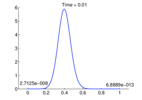
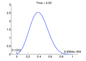
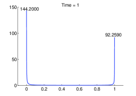
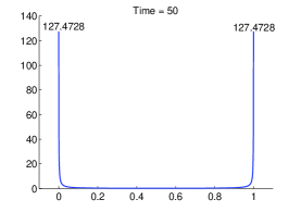
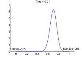
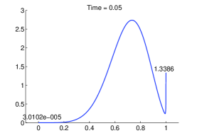
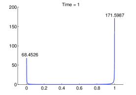
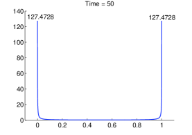
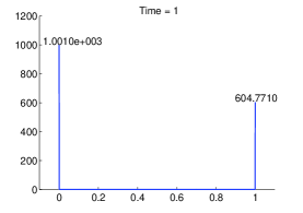
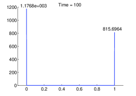
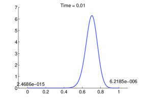
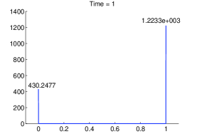
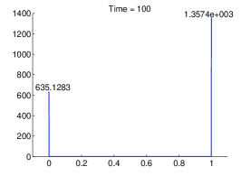
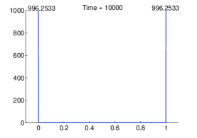
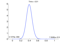
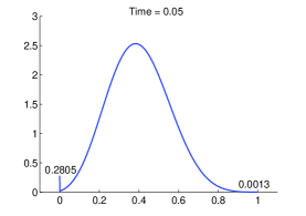
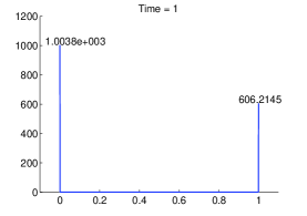
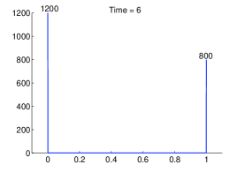
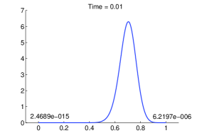
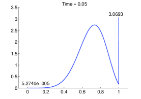
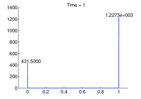
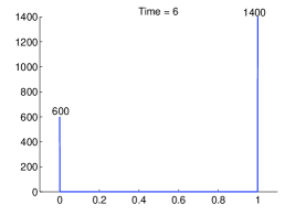
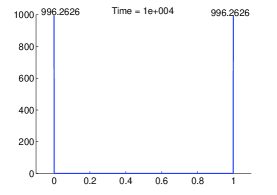
with σ<<1.much-less-than𝜎1\sigma<<1. Later, we will show the dependence on the mean value p𝑝p of the results. In Figs. 1-6 the numerical probability density at different time with various space grid sizes and initial states, are shown for all three methods. These figures show that, for all schemes, the probability density vanishes in the interval (0,1) and forms two peaks at the boundary (x=0𝑥0x=0 and x=1𝑥1x=1) as time evolves. But the heights of the peaks at the boundary at the steady state are different. For Scheme 3, the heights of the two peaks at the boundary of steady-state solution are depended on the mean of initial probability density. For Schemes 1 and 2, the heights are equals and has no relations to the expectation of initial condition. This means Schemes 1 and 2 can not keep the conservation of expectation and can not give a complete solution.

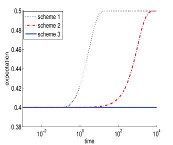
Fig. 7 shows that Scheme 3 preserves the expectation while Schemes 1 and 2 do not. This means only Scheme 3 can yield the complete solution. And it can be found that it takes a much longer time for Scheme 2 to achieve the steady state than for Scheme 1.

Table 1 presents the probability density and probability at the boundaries (f0nsuperscriptsubscript𝑓0𝑛f_{0}^{n},fMnsuperscriptsubscript𝑓𝑀𝑛f_{M}^{n} and h2f0n2superscriptsubscript𝑓0𝑛\frac{h}{2}f_{0}^{n}, h2fMn2superscriptsubscript𝑓𝑀𝑛\frac{h}{2}f_{M}^{n}), for Scheme 3 using different space grid sizes (h=1100,11000,110000110011000110000h=\frac{1}{100},\frac{1}{1000},\frac{1}{10000}) and different initial states (f(x,0)N(0.4,0.012)similar-to𝑓𝑥0𝑁0.4superscript0.012f(x,0)\sim N(0.4,0.01^{2}) and N(0.7,0.012)𝑁0.7superscript0.012N(0.7,0.01^{2})) at t=6 (τ=0.0001𝜏0.0001\tau=0.0001). It is shown that the probabilities at the boundary ends of the steady-state solution are independent of the space grid size hh. This verifies that the Dirac delta singularities do develop at the boundary points. It is also shown that the probabilities at the boundary points are depended on the expectation of the initial condition, and conservations of probability and expectation are always kept. In Table 2, for fixed grid spacing h=1/100011000h=1/1000 and two different initial states f0N(0.4,0.012)similar-tosubscript𝑓0𝑁0.4superscript0.012f_{0}\sim N(0.4,0.01^{2}) and f0N(0.7,0.012)similar-tosubscript𝑓0𝑁0.7superscript0.012f_{0}\sim N(0.7,0.01^{2}), the time step τ𝜏\tau is changed from 110110\frac{1}{10} to 110000110000\frac{1}{10000}. The results shows that Scheme 3 can get the same steady state and keep the conservation of total property and expectation for different mesh ratio γ=τh2𝛾𝜏superscript2\gamma=\frac{\tau}{h^{2}}. This means that the Scheme 3 for the genetic drift problem (4), (5), (6) and (11) is stable and independent of the mesh ratio γ𝛾\gamma, i.e. unconditional stable.
Refer to caption
Refer to caption
Refer to caption
Refer to caption
Fig. 1: Numerical results of Scheme 1 with initial state f(x,0)N(0.4,0.012)similar-to𝑓𝑥0𝑁0.4superscript0.012f(x,0)\sim N(0.4,0.01^{2}) at different time t=0.01,0.05,1,50𝑡0.010.05150t=0.01,0.05,1,50. The step sizes are h=1/1000,τ=1/1000formulae-sequence11000𝜏11000h=1/1000,\ \tau=1/1000.
Refer to caption
Refer to caption
Refer to caption
Refer to caption
Fig. 2: Numerical results of Scheme 1 with initial state f(x,0)N(0.7,0.012)similar-to𝑓𝑥0𝑁0.7superscript0.012f(x,0)\sim N(0.7,0.01^{2}) at different time t=0.01,0.05,1,50𝑡0.010.05150t=0.01,0.05,1,50. The step sizes are h=1/1000,τ=1/1000formulae-sequence11000𝜏11000h=1/1000,\ \tau=1/1000.
Refer to caption
Refer to caption
Refer to caption
Refer to caption
Fig. 3: Numerical results of Scheme 2 with initial state f(x,0)N(0.4,0.012)similar-to𝑓𝑥0𝑁0.4superscript0.012f(x,0)\sim N(0.4,0.01^{2}) at different time t=0.01,1,100,10000𝑡0.01110010000t=0.01,1,100,10000. The step sizes are h=1/1000,τ=1/1000formulae-sequence11000𝜏11000h=1/1000,\ \tau=1/1000.
Refer to caption
Refer to caption
Refer to caption
Refer to caption
Fig. 4: Numerical results of Scheme 2 with initial state f(x,0)N(0.7,0.012)similar-to𝑓𝑥0𝑁0.7superscript0.012f(x,0)\sim N(0.7,0.01^{2}) at different time t=0.01,1,100,10000𝑡0.01110010000t=0.01,1,100,10000. The step sizes are h=1/1000,τ=1/1000formulae-sequence11000𝜏11000h=1/1000,\ \tau=1/1000.
Refer to caption
Refer to caption
Refer to caption
Refer to caption
Fig. 5: Numerical results of Scheme 3 with initial state f(x,0)N(0.4,0.012)similar-to𝑓𝑥0𝑁0.4superscript0.012f(x,0)\sim N(0.4,0.01^{2}) at different time t=0.01,0.05,1,6𝑡0.010.0516t=0.01,0.05,1,6. The step sizes are h=1/1000,τ=1/1000formulae-sequence11000𝜏11000h=1/1000,\ \tau=1/1000.
Refer to caption
Refer to caption
Refer to caption
Refer to caption
Fig. 6: Numerical results of Scheme 3 with initial state f(x,0)N(0.7,0.012)similar-to𝑓𝑥0𝑁0.7superscript0.012f(x,0)\sim N(0.7,0.01^{2}) at different time t=0.01,0.05,1,6𝑡0.010.0516t=0.01,0.05,1,6. The step sizes are h=1/1000,τ=1/1000formulae-sequence11000𝜏11000h=1/1000,\ \tau=1/1000.
Refer to caption
Fig. 7: Expectation produced by different schemes with initial state f(x,0)N(0.4,0.012)similar-to𝑓𝑥0𝑁0.4superscript0.012f(x,0)\sim N(0.4,0.01^{2}) under the logarithm time scale.
space step hh N(0.4,0.012)𝑁0.4superscript0.012N(0.4,0.01^{2})
f0nsuperscriptsubscript𝑓0𝑛f_{0}^{n} fMnsuperscriptsubscript𝑓𝑀𝑛f_{M}^{n} h2f0n2superscriptsubscript𝑓0𝑛\frac{h}{2}f_{0}^{n} h2fMn2superscriptsubscript𝑓𝑀𝑛\frac{h}{2}f_{M}^{n}
1/10011001/100 1.19999123e2 7.99991237e1 0.59999562 0.39999562
1/1000110001/1000 1.19999115e3 7.99991154e2 0.59999558 0.39999558
1/100001100001/10000 1.19999115e4 7.99991146e3 0.59999557 0.39999557
space step hh N(0.7,0.012)𝑁0.7superscript0.012N(0.7,0.01^{2})
f0nsuperscriptsubscript𝑓0𝑛f_{0}^{n} fMnsuperscriptsubscript𝑓𝑀𝑛f_{M}^{n} h2f0n2superscriptsubscript𝑓0𝑛\frac{h}{2}f_{0}^{n} h2fMn2superscriptsubscript𝑓𝑀𝑛\frac{h}{2}f_{M}^{n}
1/10011001/100 5.99992332e1 1.39999236e2 0.29999617 0.69999617
1/1000110001/1000 5.99992260e2 1.39999226e3 0.29999613 0.69999613
1/100001100001/10000 5.99992253e3 1.39999225e4 0.29999613 0.69999613
Table 1: Numerical results of Scheme 3 at the boundaries at steady state (t=6𝑡6t=6, time step τ=1/10000𝜏110000\tau=1/10000) with different initial states and space grid sizes.
time step τ𝜏\tau N(0.4,0.012)𝑁0.4superscript0.012N(0.4,0.01^{2})
f0nsuperscriptsubscript𝑓0𝑛f_{0}^{n} fMnsuperscriptsubscript𝑓𝑀𝑛f_{M}^{n} h2f0n2superscriptsubscript𝑓0𝑛\frac{h}{2}f_{0}^{n} h2fMn2superscriptsubscript𝑓𝑀𝑛\frac{h}{2}f_{M}^{n}
1/101101/10 1.19997448e3 7.99974480e2 0.59998724 0.39998724
1/10011001/100 1.19999005e3 7.99990054e2 0.59999503 0.39999502
1/1000110001/1000 1.19999106e3 7.99991058e2 0.59999553 0.39999553
1/100001100001/10000 1.19999115e3 7.99991154e2 0.59999558 0.39999558
time step τ𝜏\tau N(0.7,0.012)𝑁0.7superscript0.012N(0.7,0.01^{2})
f0nsuperscriptsubscript𝑓0𝑛f_{0}^{n} fMnsuperscriptsubscript𝑓𝑀𝑛f_{M}^{n} h2f0n2superscriptsubscript𝑓0𝑛\frac{h}{2}f_{0}^{n} h2fMn2superscriptsubscript𝑓𝑀𝑛\frac{h}{2}f_{M}^{n}
1/101101/10 5.99977672e2 1.39997767e3 0.29998884 0.69998884
1/10011001/100 5.99991298e2 1.39999130e3 0.29999565 0.69999565
1/1000110001/1000 5.99992177e2 1.39999218e3 0.29999609 0.29999608
1/100001100001/10000 5.99992260e2 1.39999226e3 0.29999613 0.69999613
Table 2: Numerical results of Scheme 3 at the boundaries at steady state (t=6𝑡6t=6) with same space grid sizes h=1/100011000h=1/1000.

3.2 Analysis of Results

3.2.1 Analysis of Schemes 1 and 2

As shown in Figs. 1- 4, in the results of the first two schemes, the values of steady-state solutions at boundaries x=0𝑥0x=0 and x=1𝑥1x=1 are of the same height with different initial states. This is not consistent with the steady state of the singular solutions given in (12), and also does not satisfy the conservation of the expectation. Generally, compared to schemes without upwind technique, the upwind scheme is a better choice for the convection-diffusion problem because it is more stable due to its intrinsic numerical viscosity. It is not this case for the problem here. So we first check the effect of the numerical viscosity. To this purpose, we consider a procedure of viscosity-vanishing. First, a infinitesimal diffusion is added to the corresponding steady-state problem, then the limit behavior of the steady-state solution is investigated. Consider the following problem, for a small ϵ>0italic-ϵ0\epsilon>0,

(2) {d2dx2((x(1x)+ϵ)fϵ)=0,x(0,1),ddx((x(1x)+ϵ)fϵ)|x=0,1=0,casesformulae-sequencesuperscriptd2dsuperscript𝑥2𝑥1𝑥italic-ϵsubscript𝑓italic-ϵ0𝑥01otherwiseevaluated-atdd𝑥𝑥1𝑥italic-ϵsubscript𝑓italic-ϵ𝑥010otherwise\begin{cases}-\frac{\mathrm{d}^{2}}{\mathrm{d}x^{2}}\left((x(1-x)+\epsilon)f_{\epsilon}\right)=0,x\in(0,1),\\ \frac{\mathrm{d}}{\mathrm{d}x}\left((x(1-x)+\epsilon)f_{\epsilon}\right)\big{|}_{x=0,1}=0,\end{cases}

with a constraint 01fϵdx=1superscriptsubscript01subscript𝑓italic-ϵdifferential-d𝑥1\int_{0}^{1}\ f_{\epsilon}\ \mathrm{d}x=1. Integrating the problem (2), we get

(3) fϵ=aϵx+bϵx(1x)+ϵsubscript𝑓italic-ϵsubscript𝑎italic-ϵ𝑥subscript𝑏italic-ϵ𝑥1𝑥italic-ϵf_{\epsilon}=\frac{a_{\epsilon}x+b_{\epsilon}}{x(1-x)+\epsilon}

where aϵsubscript𝑎italic-ϵa_{\epsilon} and bϵsubscript𝑏italic-ϵb_{\epsilon} are related to ϵitalic-ϵ\epsilon. From the boundary condition,  we get aϵ=0subscript𝑎italic-ϵ0a_{\epsilon}=0. The constraint on the total probability yields that

bϵ=cϵ+lncϵ++1/2cϵ+1/2,subscript𝑏italic-ϵsuperscriptsubscript𝑐italic-ϵsuperscriptsubscript𝑐italic-ϵ12superscriptsubscript𝑐italic-ϵ12b_{\epsilon}=\frac{c_{\epsilon}^{+}}{\ln\frac{c_{\epsilon}^{+}+1/2}{c_{\epsilon}^{+}-1/2}},

where cϵ+=14+ϵ.superscriptsubscript𝑐italic-ϵ14italic-ϵc_{\epsilon}^{+}=\sqrt{\frac{1}{4}+\epsilon}. It is easy to verify that when ϵ0italic-ϵ0\epsilon\to 0,

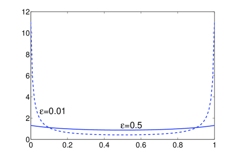
fϵ{0x(0,1)x=0,1,subscript𝑓italic-ϵcases0𝑥01𝑥01f_{\epsilon}\to\begin{cases}0&x\in(0,1)\\ \infty&x=0,1,\end{cases}

(see Fig. 6 for fϵsubscript𝑓italic-ϵf_{\epsilon}).

It is expected that fϵsubscript𝑓italic-ϵf_{\epsilon} converges to 12δ(x)+12δ(x1)12𝛿𝑥12𝛿𝑥1\frac{1}{2}\delta(x)+\frac{1}{2}\delta(x-1) in the sense of distribution. Actually we have the following theorem.
Refer to caption
Fig. 8: Two stable solution of genetic drift diffusion equation added viscosity, fϵsubscript𝑓italic-ϵf_{\epsilon}, with two different viscosities, ϵ=0.5italic-ϵ0.5\epsilon=0.5, and 0.010.010.01.
Theorem 1.

Take a zero extension of fϵsubscript𝑓italic-ϵ\ f_{\epsilon} and still denote by fϵsubscript𝑓italic-ϵ\ f_{\epsilon},

fϵ={bϵx(1x)+ϵx[0,1]0otherwise,subscript𝑓italic-ϵcasessubscript𝑏italic-ϵ𝑥1𝑥italic-ϵ𝑥010otherwisef_{\epsilon}=\begin{cases}\frac{b_{\epsilon}}{x(1-x)+\epsilon}&x\in[0,1]\\ 0&\mbox{otherwise},\end{cases}

then limϵ0+fϵφdx=12φ(0)+12φ(1)italic-ϵ0limsuperscriptsubscriptsubscript𝑓italic-ϵ𝜑differential-d𝑥12𝜑012𝜑1\underset{\epsilon\to 0}{\mathrm{lim}}\int_{-\infty}^{+\infty}\ f_{\epsilon}\varphi\ \mathrm{d}x\ =\frac{1}{2}\varphi(0)+\frac{1}{2}\varphi(1),  φC0(,)for-all𝜑superscriptsubscriptC0\ \forall\varphi\in\mathrm{C}_{0}^{\infty}(-\infty,\infty).

Proof.   For any φC0(,)𝜑superscriptsubscriptC0\varphi\in\mathrm{C}_{0}^{\infty}(-\infty,\infty)+fϵφdx=01fϵφdxsuperscriptsubscriptsubscript𝑓italic-ϵ𝜑differential-d𝑥superscriptsubscript01subscript𝑓italic-ϵ𝜑differential-d𝑥\int_{-\infty}^{+\infty}\ f_{\epsilon}\varphi\ \mathrm{d}x\ =\ \int_{0}^{1}\ f_{\epsilon}\varphi\ \mathrm{d}x
First, choosing φC0(,12)𝜑superscriptsubscriptC012\varphi\in\mathrm{C}_{0}^{\infty}(-\infty,\ \frac{1}{2}), we have

limϵ0<fϵ,φ>\displaystyle\underset{\epsilon\to 0}{\mathrm{lim}}<f_{\epsilon},\varphi>\ =\displaystyle= limϵ0012fϵφdxitalic-ϵ0limsuperscriptsubscript012subscript𝑓italic-ϵ𝜑differential-d𝑥\displaystyle\ \underset{\epsilon\to 0}{\mathrm{lim}}\int_{0}^{\frac{1}{2}}\ f_{\epsilon}\varphi\ \mathrm{d}x
=\displaystyle= limϵ0012fϵ(φ(x)φ(0))+fϵφ(0)dxitalic-ϵ0limsuperscriptsubscript012subscript𝑓italic-ϵ𝜑𝑥𝜑0subscript𝑓italic-ϵ𝜑0d𝑥\displaystyle\ \underset{\epsilon\to 0}{\mathrm{lim}}\int_{0}^{\frac{1}{2}}\ f_{\epsilon}\ (\varphi(x)-\varphi(0))+f_{\epsilon}\varphi(0)\mathrm{d}x
=\displaystyle= limϵ0012fϵ(φ(x)φ(0))dx+φ(0)012fϵdxitalic-ϵ0limsuperscriptsubscript012subscript𝑓italic-ϵ𝜑𝑥𝜑0differential-d𝑥𝜑0superscriptsubscript012subscript𝑓italic-ϵdifferential-d𝑥\displaystyle\ \underset{\epsilon\to 0}{\mathrm{lim}}\int_{0}^{\frac{1}{2}}\ f_{\epsilon}\ \left(\varphi(x)-\varphi(0)\right)\ \mathrm{d}x+\varphi(0)\int_{0}^{\frac{1}{2}}f_{\epsilon}\ \mathrm{d}x
=\displaystyle= limϵ0012fϵ(φ(x)φ(0))dx+12φ(0).italic-ϵ0limsuperscriptsubscript012subscript𝑓italic-ϵ𝜑𝑥𝜑0differential-d𝑥12𝜑0\displaystyle\ \underset{\epsilon\to 0}{\mathrm{lim}}\int_{0}^{\frac{1}{2}}\ f_{\epsilon}\ \left(\varphi(x)-\varphi(0)\right)\ \mathrm{d}x+\frac{1}{2}\varphi(0).

Now we need to prove that limϵ0012fϵ(φ(x)φ(0))dx=0italic-ϵ0limsuperscriptsubscript012subscript𝑓italic-ϵ𝜑𝑥𝜑0differential-d𝑥0\underset{\epsilon\to 0}{\mathrm{lim}}\int_{0}^{\frac{1}{2}}f_{\epsilon}\left(\varphi(x)-\varphi(0)\right)\ \mathrm{d}x=0. Denoting by cϵ=14ϵsuperscriptsubscript𝑐italic-ϵ14italic-ϵc_{\epsilon}^{-}=\sqrt{\frac{1}{4}-\epsilon} and D(x)=x(1x)𝐷𝑥𝑥1𝑥D(x)=x(1-x), we have

012fϵ(φ(x)φ(0))dxsuperscriptsubscript012subscript𝑓italic-ϵ𝜑𝑥𝜑0differential-d𝑥\displaystyle\int_{0}^{\frac{1}{2}}f_{\epsilon}\left(\varphi(x)-\varphi(0)\right)\ \mathrm{d}x =\displaystyle= 0cϵfϵ(φ(x)φ(0))dxsuperscriptsubscript0superscriptsubscript𝑐italic-ϵsubscript𝑓italic-ϵ𝜑𝑥𝜑0differential-d𝑥\displaystyle\int_{0}^{c_{\epsilon}^{-}}f_{\epsilon}\ \left(\varphi(x)-\varphi(0)\right)\ \mathrm{d}x
+cϵ12fϵ(φ(x)φ(0))dxsuperscriptsubscriptsuperscriptsubscript𝑐italic-ϵ12subscript𝑓italic-ϵ𝜑𝑥𝜑0differential-d𝑥\displaystyle+\int_{c_{\epsilon}^{-}}^{\frac{1}{2}}f_{\epsilon}\ \left(\varphi(x)-\varphi(0)\right)\ \mathrm{d}x
=superscript\displaystyle\stackrel{{\scriptstyle\bigtriangleup}}{{=}} I1+I2,subscriptI1subscriptI2\displaystyle\mathrm{I}_{1}+\mathrm{I}_{2},

where

|I1|subscriptI1\displaystyle|\mathrm{I}_{1}| =\displaystyle= |bϵ0cϵ1D(x)+ϵ(φ(x)φ(0))dx|subscript𝑏italic-ϵsuperscriptsubscript0superscriptsubscript𝑐italic-ϵ1𝐷𝑥italic-ϵ𝜑𝑥𝜑0differential-d𝑥\displaystyle\left|b_{\epsilon}\int_{0}^{c_{\epsilon}^{-}}\frac{1}{D(x)+\epsilon}\ \left(\varphi(x)-\varphi(0)\right)\ \mathrm{d}x\right|
\displaystyle\leq bϵM10cϵxD(x)+ϵdx(M1=maxx[0,12]|φ(x)|)subscript𝑏italic-ϵsubscript𝑀1superscriptsubscript0superscriptsubscript𝑐italic-ϵ𝑥𝐷𝑥italic-ϵdifferential-d𝑥subscript𝑀1subscript𝑥012superscript𝜑𝑥\displaystyle b_{\epsilon}M_{1}\int_{0}^{c_{\epsilon}^{-}}\frac{x}{D(x)+\epsilon}\ \mathrm{d}x\ \ \ (M_{1}=\max\limits_{x\in[0,\frac{1}{2}]}|\varphi^{\prime}(x)|)
\displaystyle\leq bϵM1cϵcϵcϵ(1cϵ)+ϵ0,asϵ0formulae-sequencesubscript𝑏italic-ϵsubscript𝑀1superscriptsubscript𝑐italic-ϵsuperscriptsubscript𝑐italic-ϵsuperscriptsubscript𝑐italic-ϵ1superscriptsubscript𝑐italic-ϵitalic-ϵ0asitalic-ϵ0\displaystyle b_{\epsilon}M_{1}c_{\epsilon}^{-}\frac{c_{\epsilon}^{-}}{c_{\epsilon}^{-}(1-c_{\epsilon}^{-})+\epsilon}\to 0,\qquad\mbox{as}\ \epsilon\to 0

and

|I2|subscriptI2\displaystyle|\mathrm{I}_{2}| =\displaystyle= |bϵcϵ121D(x)+ϵ(φ(x)φ(0))dx|subscript𝑏italic-ϵsubscriptsuperscript12superscriptsubscript𝑐italic-ϵ1𝐷𝑥italic-ϵ𝜑𝑥𝜑0differential-d𝑥\displaystyle\left|b_{\epsilon}\int^{\frac{1}{2}}_{c_{\epsilon}^{-}}\ \frac{1}{D(x)+\epsilon}\ \left(\varphi(x)-\varphi(0)\right)\ \mathrm{d}x\right|
\displaystyle\leq M2bϵcϵ121D(x)+ϵdx(M2=maxx[0,12]|φ(x)φ(0)|)subscript𝑀2subscript𝑏italic-ϵsubscriptsuperscript12superscriptsubscript𝑐italic-ϵ1𝐷𝑥italic-ϵdifferential-d𝑥subscript𝑀2subscript𝑥012𝜑𝑥𝜑0\displaystyle M_{2}b_{\epsilon}\int^{\frac{1}{2}}_{c_{\epsilon}^{-}}\ \frac{1}{D(x)+\epsilon}\ \mathrm{d}x\ \ \ (M_{2}=\max\limits_{x\in[0,\frac{1}{2}]}|\varphi(x)-\varphi(0)|)
=\displaystyle= bϵM212cϵlncϵ+cϵ+12cϵ++cϵ120,asϵ0.formulae-sequencesubscript𝑏italic-ϵsubscript𝑀212superscriptsubscript𝑐italic-ϵsuperscriptsubscript𝑐italic-ϵsuperscriptsubscript𝑐italic-ϵ12superscriptsubscript𝑐italic-ϵsuperscriptsubscript𝑐italic-ϵ120asitalic-ϵ0\displaystyle b_{\epsilon}M_{2}\frac{1}{2c_{\epsilon}^{-}}\ln\frac{c_{\epsilon}^{+}-c_{\epsilon}^{-}+\frac{1}{2}}{c_{\epsilon}^{+}+c_{\epsilon}^{-}-\frac{1}{2}}\to 0,\ \ \mbox{as}\ \epsilon\to 0.

Thus

(4) limϵ0<fϵ,φ>=12φ(0).formulae-sequenceitalic-ϵ0limsubscript𝑓italic-ϵ𝜑12𝜑0\underset{\epsilon\to 0}{\mathrm{lim}}<f_{\epsilon},\varphi>\ =\frac{1}{2}\varphi(0).

Similarly, choosing φC0(12,)𝜑superscriptsubscriptC012\varphi\in\mathrm{C}_{0}^{\infty}(\frac{1}{2},\ \infty),  we get

(5) limϵ0<fϵ,φ>=12φ(1).formulae-sequenceitalic-ϵ0limsubscript𝑓italic-ϵ𝜑12𝜑1\underset{\epsilon\to 0}{\mathrm{lim}}<f_{\epsilon},\varphi>\ =\frac{1}{2}\varphi(1).

Combining together,  we have that limϵ0<fϵ,φ>=12φ(0)+12φ(1)formulae-sequenceitalic-ϵ0limsubscript𝑓italic-ϵ𝜑12𝜑012𝜑1\underset{\epsilon\to 0}{\mathrm{lim}}<f_{\epsilon},\varphi>\ =\frac{1}{2}\varphi(0)+\frac{1}{2}\varphi(1), for φ(x)C0(,)for-all𝜑𝑥superscriptsubscriptC0\forall\varphi(x)\in\mathrm{C}_{0}^{\infty}(-\infty,\infty). The proof is completed. \blacksquare

We see that the long time behavior of the original problem will be changed by any extra infinitesimal viscosity since the steady-state solution always is δ(x)/2+δ(1x)/2𝛿𝑥2𝛿1𝑥2\delta(x)/2+\delta(1-x)/2, no matter what the initial state is. It means that the conservation of expectation must be destroyed by any extra viscosity. This is consistent with the results showed in Figs. 1 and 2 for Scheme 1, since we know that the upwind scheme always introduces a first order viscosity into a central difference scheme.

However, numerical results in Figs. 3 and 4 show that the central difference scheme (Scheme 2) is stable for this convection-dominated problem and the values of steady-state solutions at boundaries x=0𝑥0x=0 and x=1𝑥1x=1 are of the same height with different initial states, which also destroy the conservation of the expectation. Turning to Figs 5 and 6, for the other central scheme (Scheme 3), we have stable and correct long time behavior. In the next subsection, we will prove the stability and long-time convergence for Scheme 3. Taking the difference between these schemes, we will get the answer for these different observations.

Theorem 2.

Scheme 2: (1), (2) and (6) can be rewritten in the following form as

(6) finfin1τDi+1fi+1n2Difin+Di1fi1nh2+Λ=0subscriptsuperscript𝑓𝑛𝑖subscriptsuperscript𝑓𝑛1𝑖𝜏subscript𝐷𝑖1subscriptsuperscript𝑓𝑛𝑖12subscript𝐷𝑖subscriptsuperscript𝑓𝑛𝑖subscript𝐷𝑖1subscriptsuperscript𝑓𝑛𝑖1superscript2Λ0\displaystyle\frac{f^{n}_{i}-f^{n-1}_{i}}{\tau}-\frac{D_{i+1}f^{n}_{i+1}-2D_{i}f^{n}_{i}+D_{i-1}f^{n}_{i-1}}{h^{2}}+\Lambda=0

and Scheme 1: (1), (2) and (5) can be rewritten in the following form as

(7) finfin1τDi+1fi+1n2Difin+Di1fi1nh2+Λ+Λ~=0,subscriptsuperscript𝑓𝑛𝑖subscriptsuperscript𝑓𝑛1𝑖𝜏subscript𝐷𝑖1subscriptsuperscript𝑓𝑛𝑖12subscript𝐷𝑖subscriptsuperscript𝑓𝑛𝑖subscript𝐷𝑖1subscriptsuperscript𝑓𝑛𝑖1superscript2Λ~Λ0\displaystyle\frac{f^{n}_{i}-f^{n-1}_{i}}{\tau}-\frac{D_{i+1}f^{n}_{i+1}-2D_{i}f^{n}_{i}+D_{i-1}f^{n}_{i-1}}{h^{2}}+\Lambda+\tilde{\Lambda}=0,

with

Λ=h24fi+1n2fin+fi1nh2,Λ~=h2|bi+12|fi+1n(|bi+12|+|bi12)|fin+|bi12|fi1nh2,\Lambda=-\frac{h^{2}}{4}\frac{f^{n}_{i+1}-2f^{n}_{i}+f^{n}_{i-1}}{h^{2}},\ \ \tilde{\Lambda}=-\frac{h}{2}\frac{|b_{i+\frac{1}{2}}|f_{i+1}^{n}-(|b_{i+\frac{1}{2}}|+|b_{i-\frac{1}{2}})|f^{n}_{i}+|b_{i-\frac{1}{2}}|f^{n}_{i-1}}{h^{2}},

where D(x)=x(1x)𝐷𝑥𝑥1𝑥D(x)=x(1-x) and b(x)=Dx=12x𝑏𝑥subscript𝐷𝑥12𝑥b(x)=D_{x}=1-2x.

Theorem 2 tells us that Scheme 2 is just Scheme 3 plus a second order (of O(h2)𝑂superscript2O(h^{2})) viscosity term and for Scheme 1, another first order viscosity term is introduced in. That is the reason why Scheme 2 is also stable and it takes a much longer time for Scheme 2 than for Scheme 1 to achieve the same wrong steady state.

Proof of Theorem 2. ΛΛ\Lambda is the difference between Schemes 2 and 3. We have after direct computation that

(8) ΛΛ\displaystyle\ \ \ \ \Lambda =\displaystyle= 1h2((Di+1Di+12)fi+1n+(Di+12+Di122Di)fin+(Di1Di12)fi1n)1superscript2subscript𝐷𝑖1subscript𝐷𝑖12superscriptsubscript𝑓𝑖1𝑛subscript𝐷𝑖12subscript𝐷𝑖122subscript𝐷𝑖subscriptsuperscript𝑓𝑛𝑖subscript𝐷𝑖1subscript𝐷𝑖12subscriptsuperscript𝑓𝑛𝑖1\displaystyle\frac{1}{h^{2}}\left((D_{i+1}-D_{i+\frac{1}{2}})f_{i+1}^{n}+(D_{i+\frac{1}{2}}+D_{i-\frac{1}{2}}-2D_{i})f^{n}_{i}+(D_{i-1}-D_{i-\frac{1}{2}})f^{n}_{i-1}\right)
bi+12fi+1n+(bi+12bi12)finbi12fi1n2hsubscript𝑏𝑖12subscriptsuperscript𝑓𝑛𝑖1subscript𝑏𝑖12subscript𝑏𝑖12subscriptsuperscript𝑓𝑛𝑖subscript𝑏𝑖12subscriptsuperscript𝑓𝑛𝑖12\displaystyle-\frac{b_{i+\frac{1}{2}}f^{n}_{i+1}+(b_{i+\frac{1}{2}}-b_{i-\frac{1}{2}})f^{n}_{i}-b_{i-\frac{1}{2}}f^{n}_{i-1}}{2h}
=\displaystyle= 1h2((Di+1Di+12h2bi+12)fi+1n+(Di1Di12+bi12)fi1n)1superscript2subscript𝐷𝑖1subscript𝐷𝑖122subscript𝑏𝑖12superscriptsubscript𝑓𝑖1𝑛subscript𝐷𝑖1subscript𝐷𝑖12subscript𝑏𝑖12subscriptsuperscript𝑓𝑛𝑖1\displaystyle\frac{1}{h^{2}}\left((D_{i+1}-D_{i+\frac{1}{2}}-\frac{h}{2}b_{i+\frac{1}{2}})f_{i+1}^{n}+(D_{i-1}-D_{i-\frac{1}{2}}+b_{i-\frac{1}{2}})f^{n}_{i-1}\right)
+1h2((Di+12+Di122Di(bi+12bi12))fin)1superscript2subscript𝐷𝑖12subscript𝐷𝑖122subscript𝐷𝑖subscript𝑏𝑖12subscript𝑏𝑖12subscriptsuperscript𝑓𝑛𝑖\displaystyle+\frac{1}{h^{2}}\left((D_{i+\frac{1}{2}}+D_{i-\frac{1}{2}}-2D_{i}-(b_{i+\frac{1}{2}}-b_{i-\frac{1}{2}}))f^{n}_{i}\right)
=\displaystyle= 1h2(h28Dxxfi+1n+h28Dxxfi1nh24Dxxfin)1superscript2superscript28subscript𝐷𝑥𝑥subscriptsuperscript𝑓𝑛𝑖1superscript28subscript𝐷𝑥𝑥subscriptsuperscript𝑓𝑛𝑖1superscript24subscript𝐷𝑥𝑥subscriptsuperscript𝑓𝑛𝑖\displaystyle\frac{1}{h^{2}}\left(\frac{h^{2}}{8}D_{xx}f^{n}_{i+1}+\frac{h^{2}}{8}D_{xx}f^{n}_{i-1}-\frac{h^{2}}{4}D_{xx}f^{n}_{i}\right)
=\displaystyle= h24fi+1n2fin+fi1nh2,superscript24subscriptsuperscript𝑓𝑛𝑖12subscriptsuperscript𝑓𝑛𝑖subscriptsuperscript𝑓𝑛𝑖1superscript2\displaystyle-\frac{h^{2}}{4}\frac{f^{n}_{i+1}-2f^{n}_{i}+f^{n}_{i-1}}{h^{2}},

where we have used the facts that Dxx=2subscript𝐷𝑥𝑥2D_{xx}=-2 and dndxnD=0,n>2formulae-sequencesuperscript𝑑𝑛𝑑superscript𝑥𝑛𝐷0𝑛2\frac{d^{n}}{dx^{n}}D=0,~{}n>2.

Note that Λ~~Λ\tilde{\Lambda} is the difference between Schemes 1 and 2, which, as we have known, is a first order viscosity term introduced by a upwind scheme ([3, 17]). For completeness, we derive it again. There are only 3 situations to check.

Case 1: 0bi12<bi+120subscript𝑏𝑖12subscript𝑏𝑖120\leq b_{i-\frac{1}{2}}<b_{i+\frac{1}{2}}.

(9) Λ~~Λ\displaystyle\tilde{\Lambda} =\displaystyle= bi+12fi+1n+(bi+12bi12)finbi12fi1n2hbi+12fi+1nbi12finhsubscript𝑏𝑖12subscriptsuperscript𝑓𝑛𝑖1subscript𝑏𝑖12subscript𝑏𝑖12subscriptsuperscript𝑓𝑛𝑖subscript𝑏𝑖12subscriptsuperscript𝑓𝑛𝑖12subscript𝑏𝑖12superscriptsubscript𝑓𝑖1𝑛subscript𝑏𝑖12superscriptsubscript𝑓𝑖𝑛\displaystyle\frac{b_{i+\frac{1}{2}}f^{n}_{i+1}+(b_{i+\frac{1}{2}}-b_{i-\frac{1}{2}})f^{n}_{i}-b_{i-\frac{1}{2}}f^{n}_{i-1}}{2h}-\frac{b_{i+\frac{1}{2}}f_{i+1}^{n}-b_{i-\frac{1}{2}}f_{i}^{n}}{h}
=\displaystyle= bi+12fi+1n+(bi+12bi12)finbi12fi1n2hsubscript𝑏𝑖12subscriptsuperscript𝑓𝑛𝑖1subscript𝑏𝑖12subscript𝑏𝑖12subscriptsuperscript𝑓𝑛𝑖subscript𝑏𝑖12subscriptsuperscript𝑓𝑛𝑖12\displaystyle\frac{-b_{i+\frac{1}{2}}f^{n}_{i+1}+(b_{i+\frac{1}{2}}-b_{i-\frac{1}{2}})f^{n}_{i}-b_{i-\frac{1}{2}}f^{n}_{i-1}}{2h}
=\displaystyle= h2bi+12fi+1n(bi+12+bi12)fin+bi12fi1nh2.2subscript𝑏𝑖12subscriptsuperscript𝑓𝑛𝑖1subscript𝑏𝑖12subscript𝑏𝑖12subscriptsuperscript𝑓𝑛𝑖subscript𝑏𝑖12subscriptsuperscript𝑓𝑛𝑖1superscript2\displaystyle-\frac{h}{2}\frac{b_{i+\frac{1}{2}}f^{n}_{i+1}-(b_{i+\frac{1}{2}}+b_{i-\frac{1}{2}})f^{n}_{i}+b_{i-\frac{1}{2}}f^{n}_{i-1}}{h^{2}}.

Case 2: bi12<bi+120subscript𝑏𝑖12subscript𝑏𝑖120b_{i-\frac{1}{2}}<b_{i+\frac{1}{2}}\leq 0.

(10) Λ~~Λ\displaystyle\tilde{\Lambda} =\displaystyle= h2bi+12fi+1n+(bi+12+bi12)finbi12fi1nh2.2subscript𝑏𝑖12subscriptsuperscript𝑓𝑛𝑖1subscript𝑏𝑖12subscript𝑏𝑖12subscriptsuperscript𝑓𝑛𝑖subscript𝑏𝑖12subscriptsuperscript𝑓𝑛𝑖1superscript2\displaystyle-\frac{h}{2}\frac{-b_{i+\frac{1}{2}}f^{n}_{i+1}+(b_{i+\frac{1}{2}}+b_{i-\frac{1}{2}})f^{n}_{i}-b_{i-\frac{1}{2}}f^{n}_{i-1}}{h^{2}}.

Case 3: bi120bi+12subscript𝑏𝑖120subscript𝑏𝑖12b_{i-\frac{1}{2}}\leq 0\leq b_{i+\frac{1}{2}}.

(11) Λ~~Λ\displaystyle\tilde{\Lambda} =\displaystyle= h2bi+12fi+1n(bi+12bi12)finbi12fi1nh2.2subscript𝑏𝑖12subscriptsuperscript𝑓𝑛𝑖1subscript𝑏𝑖12subscript𝑏𝑖12subscriptsuperscript𝑓𝑛𝑖subscript𝑏𝑖12subscriptsuperscript𝑓𝑛𝑖1superscript2\displaystyle-\frac{h}{2}\frac{b_{i+\frac{1}{2}}f^{n}_{i+1}-(b_{i+\frac{1}{2}}-b_{i-\frac{1}{2}})f^{n}_{i}-b_{i-\frac{1}{2}}f^{n}_{i-1}}{h^{2}}.

Combining all together, we get

Λ~=h2|bi+12|fi+1n(|bi+12|+|bi12)|fin+|bi12|fi1nh2.\tilde{\Lambda}=-\frac{h}{2}\frac{|b_{i+\frac{1}{2}}|f_{i+1}^{n}-(|b_{i+\frac{1}{2}}|+|b_{i-\frac{1}{2}})|f^{n}_{i}+|b_{i-\frac{1}{2}}|f^{n}_{i-1}}{h^{2}}.

The proof is completed. \blacksquare

3.2.2 Analysis of Scheme 3

In this section, we will prove the stability and long-time convergence for Scheme 3. (1), (2) and (7) can be split into three independent parts. For inner points, i=1,,M1,𝑖1𝑀1i=1,\cdots,M-1,

(12) fin+1finτDi+1fi+1n+12Difin+1+Di1fi1n+1h2=0,subscriptsuperscript𝑓𝑛1𝑖subscriptsuperscript𝑓𝑛𝑖𝜏subscript𝐷𝑖1subscriptsuperscript𝑓𝑛1𝑖12subscript𝐷𝑖subscriptsuperscript𝑓𝑛1𝑖subscript𝐷𝑖1subscriptsuperscript𝑓𝑛1𝑖1superscript20\displaystyle\frac{f^{n+1}_{i}-f^{n}_{i}}{\tau}-\frac{D_{i+1}f^{n+1}_{i+1}-2D_{i}f^{n+1}_{i}+D_{i-1}f^{n+1}_{i-1}}{h^{2}}=0,~{}

with Di=xi(1xi)subscript𝐷𝑖subscript𝑥𝑖1subscript𝑥𝑖D_{i}=x_{i}(1-x_{i}). For the boundary points, it yields,

(13) f0n+1=f0n+2D1γf1n+1,subscriptsuperscript𝑓𝑛10subscriptsuperscript𝑓𝑛02subscript𝐷1𝛾subscriptsuperscript𝑓𝑛11\displaystyle f^{n+1}_{0}=f^{n}_{0}+2D_{1}\gamma f^{n+1}_{1},
(14) fMn+1=fMn+2DM1γfM1n+1,subscriptsuperscript𝑓𝑛1𝑀subscriptsuperscript𝑓𝑛𝑀2subscript𝐷𝑀1𝛾subscriptsuperscript𝑓𝑛1𝑀1\displaystyle f^{n+1}_{M}=f^{n}_{M}+2D_{M-1}\gamma f^{n+1}_{M-1},

with the mesh ratio γ=τh2𝛾𝜏superscript2\gamma=\frac{\tau}{h^{2}}.

Due to D0=DM=0subscript𝐷0subscript𝐷𝑀0D_{0}=D_{M}=0, the unknowns at inner points f1n+1,,fM1n+1subscriptsuperscript𝑓𝑛11subscriptsuperscript𝑓𝑛1𝑀1f^{n+1}_{1},\cdots,f^{n+1}_{M-1} form a closed linear system which can be solved first. Then the boundary points f0n+1,fMn+1subscriptsuperscript𝑓𝑛10subscriptsuperscript𝑓𝑛1𝑀f^{n+1}_{0},f^{n+1}_{M} can be updated by the inner points f1n+1,fM1n+1subscriptsuperscript𝑓𝑛11subscriptsuperscript𝑓𝑛1𝑀1f^{n+1}_{1},~{}f^{n+1}_{M-1} respectively.

In the following, we prove FVM keeps discrete total probability and Scheme 3 also preserves the expectation. The discrete total probability and expectation at step n𝑛n are defined as follows.

(15) Pnsubscript𝑃𝑛\displaystyle P_{n} =\displaystyle= h2f0n+h2fMn+i=1M1finh,2superscriptsubscript𝑓0𝑛2superscriptsubscript𝑓𝑀𝑛superscriptsubscript𝑖1𝑀1superscriptsubscript𝑓𝑖𝑛\displaystyle\frac{h}{2}f_{0}^{n}+\frac{h}{2}f_{M}^{n}+\sum_{i=1}^{M-1}f_{i}^{n}h,
(16) Ensubscript𝐸𝑛\displaystyle E_{n} =\displaystyle= h2x0f0n+h2xMfMn+i=1M1xifinh,2subscript𝑥0superscriptsubscript𝑓0𝑛2subscript𝑥𝑀superscriptsubscript𝑓𝑀𝑛superscriptsubscript𝑖1𝑀1subscript𝑥𝑖superscriptsubscript𝑓𝑖𝑛\displaystyle\frac{h}{2}x_{0}f_{0}^{n}+\frac{h}{2}x_{M}f_{M}^{n}+\sum_{i=1}^{M-1}x_{i}f_{i}^{n}h,
Lemma 3.

For the genetic drift problem (4), (5), (6) and (11), the finite volume method (1), (2) keep the discrete total probability, Pn+1=Pnsubscript𝑃𝑛1subscript𝑃𝑛P_{n+1}=P_{n}. Furthermore, the central finite volume method (7) yields a complete solution, which preserves the discrete expectation, En+1=Ensubscript𝐸𝑛1subscript𝐸𝑛E_{n+1}=E_{n}.

Proof. By the definition of Pnsubscript𝑃𝑛P_{n}, it yields,

(17) Pn+1Pn=h2(f0n+1f0n)+h2(fMn+1fMn)+i=1M1(fin+1fin)h.subscript𝑃𝑛1subscript𝑃𝑛2superscriptsubscript𝑓0𝑛1superscriptsubscript𝑓0𝑛2superscriptsubscript𝑓𝑀𝑛1superscriptsubscript𝑓𝑀𝑛superscriptsubscript𝑖1𝑀1superscriptsubscript𝑓𝑖𝑛1superscriptsubscript𝑓𝑖𝑛P_{n+1}-P_{n}=\frac{h}{2}(f_{0}^{n+1}-f_{0}^{n})+\frac{h}{2}(f_{M}^{n+1}-f_{M}^{n})+\sum_{i=1}^{M-1}(f_{i}^{n+1}-f_{i}^{n})h.

Using (1) and (2), we have

(18) Pn+1Pnsubscript𝑃𝑛1subscript𝑃𝑛\displaystyle P_{n+1}-P_{n} =\displaystyle= τi=1M1(ji+12n+1ji12n+1)τj12n+1+τjM12n+1=0.𝜏superscriptsubscript𝑖1𝑀1superscriptsubscript𝑗𝑖12𝑛1superscriptsubscript𝑗𝑖12𝑛1𝜏superscriptsubscript𝑗12𝑛1𝜏superscriptsubscript𝑗𝑀12𝑛10\displaystyle-\tau\sum_{i=1}^{M-1}(j_{i+\frac{1}{2}}^{n+1}-j_{i-\frac{1}{2}}^{n+1})-\tau j_{\frac{1}{2}}^{n+1}+\tau j_{M-\frac{1}{2}}^{n+1}=0.

On the other hand,

(19) En+1En=h2x0(f0n+1f0n)+h2xM(fMn+1fMn)+i=1M1xi(fin+1fin)h.subscript𝐸𝑛1subscript𝐸𝑛2subscript𝑥0superscriptsubscript𝑓0𝑛1superscriptsubscript𝑓0𝑛2subscript𝑥𝑀superscriptsubscript𝑓𝑀𝑛1superscriptsubscript𝑓𝑀𝑛superscriptsubscript𝑖1𝑀1subscript𝑥𝑖superscriptsubscript𝑓𝑖𝑛1superscriptsubscript𝑓𝑖𝑛E_{n+1}-E_{n}=\frac{h}{2}x_{0}(f_{0}^{n+1}-f_{0}^{n})+\frac{h}{2}x_{M}(f_{M}^{n+1}-f_{M}^{n})+\sum_{i=1}^{M-1}x_{i}(f_{i}^{n+1}-f_{i}^{n})h.

Using (1) and (2), we have

(20) En+1Ensubscript𝐸𝑛1subscript𝐸𝑛\displaystyle E_{n+1}-E_{n} =\displaystyle= τi=1M1xi(ji+12n+1ji12n+1)+τxMjM12n+1𝜏superscriptsubscript𝑖1𝑀1subscript𝑥𝑖superscriptsubscript𝑗𝑖12𝑛1superscriptsubscript𝑗𝑖12𝑛1𝜏subscript𝑥𝑀superscriptsubscript𝑗𝑀12𝑛1\displaystyle-\tau\sum_{i=1}^{M-1}x_{i}(j_{i+\frac{1}{2}}^{n+1}-j_{i-\frac{1}{2}}^{n+1})+\tau x_{M}j_{M-\frac{1}{2}}^{n+1}\ \ \
=\displaystyle= hτi=1M1ji+12n+1.𝜏superscriptsubscript𝑖1𝑀1superscriptsubscript𝑗𝑖12𝑛1\displaystyle h\tau\sum_{i=1}^{M-1}j_{i+\frac{1}{2}}^{n+1}.

Combining with (7), we get

(21) i=1M1ji+12n+1=0.superscriptsubscript𝑖1𝑀1superscriptsubscript𝑗𝑖12𝑛10\sum_{i=1}^{M-1}j_{i+\frac{1}{2}}^{n+1}=0.

Thus, for Scheme 3, En+1=Ensubscript𝐸𝑛1subscript𝐸𝑛E_{n+1}=E_{n}. The proof is completed. \blacksquare

Lemma 4.

Let finsuperscriptsubscript𝑓𝑖𝑛f_{i}^{n} be the solution of Scheme 3: (1), (2) and (7). Then,

i=1M1xifin+1hi=1M1fin+1heπ2tn+144h(1h)i=1M1fi0h,tn+1=(n+1)τ.formulae-sequencesuperscriptsubscript𝑖1𝑀1subscript𝑥𝑖superscriptsubscript𝑓𝑖𝑛1superscriptsubscript𝑖1𝑀1superscriptsubscript𝑓𝑖𝑛1superscript𝑒superscript𝜋2subscript𝑡𝑛1441superscriptsubscript𝑖1𝑀1superscriptsubscript𝑓𝑖0subscript𝑡𝑛1𝑛1𝜏\sum_{i=1}^{M-1}x_{i}f_{i}^{n+1}h\leq\sum_{i=1}^{M-1}f_{i}^{n+1}h\leq\frac{e^{-\frac{\pi^{2}t_{n+1}}{4}}}{4h(1-h)}\sum_{i=1}^{M-1}f_{i}^{0}h,~{}t_{n+1}=(n+1)\tau.

Proof. Since Di=xi(1xi)>0subscript𝐷𝑖subscript𝑥𝑖1subscript𝑥𝑖0D_{i}=x_{i}(1-x_{i})>0 for i=1,,M1𝑖1𝑀1i=1,\cdots,M-1, by setting vin=Difinsuperscriptsubscript𝑣𝑖𝑛subscript𝐷𝑖superscriptsubscript𝑓𝑖𝑛v_{i}^{n}=D_{i}f_{i}^{n}, Scheme 3 for inner points (12) can be rewritten as

(22) 1Divin+1vinτvi+1n+12vin+1+vi1n+1h2=0.1subscript𝐷𝑖superscriptsubscript𝑣𝑖𝑛1superscriptsubscript𝑣𝑖𝑛𝜏superscriptsubscript𝑣𝑖1𝑛12superscriptsubscript𝑣𝑖𝑛1superscriptsubscript𝑣𝑖1𝑛1superscript20\frac{1}{D_{i}}\frac{v_{i}^{n+1}-v_{i}^{n}}{\tau}-\frac{v_{i+1}^{n+1}-2v_{i}^{n+1}+v_{i-1}^{n+1}}{h^{2}}=0.

It is obviously that the discrete maximum principle is valid. So we have

(23) vin0,fin0,i=1,,M1,n>1,formulae-sequencesuperscriptsubscript𝑣𝑖𝑛0formulae-sequencesuperscriptsubscript𝑓𝑖𝑛0formulae-sequence𝑖1𝑀1𝑛1v_{i}^{n}\geq 0,\ \ f_{i}^{n}\geq 0,\ \ i=1,\cdots,M-1,\ n>1,

since the initial value is nonnegative.

Multiplying by vin+1hsuperscriptsubscript𝑣𝑖𝑛1v_{i}^{n+1}h on both sides of (22), summing from i=1𝑖1i=1 to M1𝑀1M-1, using Hölder inequality and D(x)14𝐷𝑥14D(x)\leq\frac{1}{4}, it yields that

(24) 2vin+1h2τi=1M1vi+1n+12vin+1+vi1n+1h2vin+1h2vinh2τ,2subscriptsuperscriptnormsuperscriptsubscript𝑣𝑖𝑛12𝜏superscriptsubscript𝑖1𝑀1superscriptsubscript𝑣𝑖1𝑛12superscriptsubscript𝑣𝑖𝑛1superscriptsubscript𝑣𝑖1𝑛1superscript2superscriptsubscript𝑣𝑖𝑛12subscriptsuperscriptnormsuperscriptsubscript𝑣𝑖𝑛2𝜏2\frac{\|v_{i}^{n+1}\|^{2}_{h}}{\tau}-\sum_{i=1}^{M-1}\frac{v_{i+1}^{n+1}-2v_{i}^{n+1}+v_{i-1}^{n+1}}{h^{2}}v_{i}^{n+1}h\leq 2\frac{\|v_{i}^{n}\|^{2}_{h}}{\tau},

where vnh=(i=1M1|vin|2h)1/2subscriptnormsuperscript𝑣𝑛superscriptsuperscriptsubscript𝑖1𝑀1superscriptsuperscriptsubscript𝑣𝑖𝑛212\displaystyle\|v^{n}\|_{h}=\left(\sum_{i=1}^{M-1}|v_{i}^{n}|^{2}h\right)^{1/2} is the discrete L2superscript𝐿2L^{2} norm of vnsubscript𝑣𝑛v_{n}.

Denote by Δhwi=wi12wi+wi+1h2subscriptΔsubscript𝑤𝑖subscript𝑤𝑖12subscript𝑤𝑖subscript𝑤𝑖1superscript2{\displaystyle\Delta_{h}w_{i}=\frac{w_{i-1}-2w_{i}+w_{i+1}}{h^{2}}} the discrete Laplacian. We know that the minimum eigenvalue of the problem

Δhwi=λwi,i=1,,M1,w0=wM=0,formulae-sequencesubscriptΔsubscript𝑤𝑖𝜆subscript𝑤𝑖formulae-sequence𝑖1𝑀1subscript𝑤0subscript𝑤𝑀0-\Delta_{h}w_{i}=\lambda w_{i},\ \ i=1,\cdots,M-1,\ \ w_{0}=w_{M}=0,

is λ0=4h2sin2(π2M)subscript𝜆04superscript2superscript2𝜋2𝑀\lambda_{0}=\frac{4}{h^{2}}\sin^{2}(\frac{\pi}{2M}). Then from (24),

(25) 2vin+1h2τ+λ0vn+1h22vinh2τ.2subscriptsuperscriptnormsuperscriptsubscript𝑣𝑖𝑛12𝜏subscript𝜆0superscriptsubscriptnormsuperscript𝑣𝑛122subscriptsuperscriptnormsuperscriptsubscript𝑣𝑖𝑛2𝜏2\frac{\|v_{i}^{n+1}\|^{2}_{h}}{\tau}+\lambda_{0}\|v^{n+1}\|_{h}^{2}\leq 2\frac{\|v_{i}^{n}\|^{2}_{h}}{\tau}.

So we get the estimate

(26) vn+1h2(11+τλ02)vnh2eπ2tn+12v0h2,tn+1=(n+1)τ.formulae-sequencesuperscriptsubscriptnormsuperscript𝑣𝑛1211𝜏subscript𝜆02superscriptsubscriptnormsuperscript𝑣𝑛2superscript𝑒superscript𝜋2subscript𝑡𝑛12superscriptsubscriptnormsuperscript𝑣02subscript𝑡𝑛1𝑛1𝜏\|v^{n+1}\|_{h}^{2}\leq\left(\frac{1}{1+\frac{\tau\lambda_{0}}{2}}\right)\|v^{n}\|_{h}^{2}\leq e^{-\frac{\pi^{2}t_{n+1}}{2}}\|v^{0}\|_{h}^{2},~{}t_{n+1}=(n+1)\tau.

By Hölder inequality, above formula means,

(27) i=1M1vin+1h(i=1M1|vin+1|2h)1/2=vn+1heπ2tn+14v0h.superscriptsubscript𝑖1𝑀1superscriptsubscript𝑣𝑖𝑛1superscriptsuperscriptsubscript𝑖1𝑀1superscriptsuperscriptsubscript𝑣𝑖𝑛1212subscriptnormsuperscript𝑣𝑛1superscript𝑒superscript𝜋2subscript𝑡𝑛14subscriptnormsuperscript𝑣0\sum_{i=1}^{M-1}v_{i}^{n+1}h\leq(\sum_{i=1}^{M-1}|v_{i}^{n+1}|^{2}h)^{1/2}=\|v^{n+1}\|_{h}\leq e^{-\frac{\pi^{2}t_{n+1}}{4}}\|v^{0}\|_{h}.

For fixed grid spacing hh, h(1h)Di141subscript𝐷𝑖14h(1-h)\leq D_{i}\leq\frac{1}{4}, i=1,,M1𝑖1𝑀1i=1,\cdots,M-1. Thanks to vin+1=Difin+1superscriptsubscript𝑣𝑖𝑛1subscript𝐷𝑖superscriptsubscript𝑓𝑖𝑛1v_{i}^{n+1}=D_{i}f_{i}^{n+1}, fin+1superscriptsubscript𝑓𝑖𝑛1f_{i}^{n+1} can be estimated as follows:

(28) i=1M1fin+1heπ2tn+144h(1h)i=1M1fi0h.superscriptsubscript𝑖1𝑀1superscriptsubscript𝑓𝑖𝑛1superscript𝑒superscript𝜋2subscript𝑡𝑛1441superscriptsubscript𝑖1𝑀1superscriptsubscript𝑓𝑖0\sum_{i=1}^{M-1}f_{i}^{n+1}h\leq\frac{e^{-\frac{\pi^{2}t_{n+1}}{4}}}{4h(1-h)}\sum_{i=1}^{M-1}f_{i}^{0}h.

At the same time, since x(0,1)𝑥01x\in(0,1), by (28), we can directly obtain,

(29) i=1M1xifin+1hi=1M1fin+1heπ2tn+144h(1h)i=1M1fi0h.superscriptsubscript𝑖1𝑀1subscript𝑥𝑖superscriptsubscript𝑓𝑖𝑛1superscriptsubscript𝑖1𝑀1superscriptsubscript𝑓𝑖𝑛1superscript𝑒superscript𝜋2subscript𝑡𝑛1441superscriptsubscript𝑖1𝑀1superscriptsubscript𝑓𝑖0\sum_{i=1}^{M-1}x_{i}f_{i}^{n+1}h\leq\sum_{i=1}^{M-1}f_{i}^{n+1}h\leq\frac{e^{-\frac{\pi^{2}t_{n+1}}{4}}}{4h(1-h)}\sum_{i=1}^{M-1}f_{i}^{0}h.

The proof is completed. \blacksquare

Theorem 5.

Scheme 3: (1), (2) and (7) is unconditionally stable and for fixed hh and τ𝜏\tau and we have, as n𝑛n\rightarrow\infty, that

(30) {fin0,fori=1,,M1,h2f0n+h2fMnP0,h2xMfMnE0,casesformulae-sequencesuperscriptsubscript𝑓𝑖𝑛0for𝑖1𝑀12superscriptsubscript𝑓0𝑛2superscriptsubscript𝑓𝑀𝑛subscript𝑃02subscript𝑥𝑀superscriptsubscript𝑓𝑀𝑛subscript𝐸0\left\{\begin{array}[]{l}f_{i}^{n}\rightarrow 0,~{}\mbox{for}~{}i=1,\cdots,M-1,\\ \frac{h}{2}f_{0}^{n}+\frac{h}{2}f_{M}^{n}\rightarrow P_{0},\\ \frac{h}{2}x_{M}f_{M}^{n}\rightarrow E_{0},\end{array}\right.

i.e.,

(31) {h2f0n(P0E0)1p,h2fMnE0p.cases2superscriptsubscript𝑓0𝑛subscript𝑃0subscript𝐸01𝑝2superscriptsubscript𝑓𝑀𝑛subscript𝐸0𝑝\left\{\begin{array}[]{l}\frac{h}{2}f_{0}^{n}\rightarrow(P_{0}-E_{0})\approx 1-p,\\ \frac{h}{2}f_{M}^{n}\rightarrow E_{0}\approx p.\end{array}\right.

Proof. The unconditional stability is ensured by the discrete maximum principle. The long-time convergence comes from Lemmas 3, 4 and nonnegative property of the solution (23). The proof is completed. \blacksquare

4 Conclusion and discussion

We have considered three different numerical schemes for genetic drift diffusion equation. Schemes 1 and 2 discritize the flux in convection and diffusion form using upwind and central difference methods, respectively. Scheme 3 discritizes the flux as a whole using cental difference method. Numerical experiments show that all the schemes are stable and the first two schemes give an artificial steady state solution while Scheme 3 presents the correct one. Analysis shows that Scheme 3 preserves both of total probability and expectation, so it yields the complete solution. We prove that any extra infinitesimal diffusion leads to a same steady state. We find that Scheme 2, also a central scheme, introduces a second order numerical viscosity term to Scheme 3, while Scheme 1, as a upwind one, introduces another first order numerical viscosity term to Scheme 2. Therefore, both Schemes 1 and 2 yield the same artificial long time behaviors of the numerical solutions, but it takes different time for them to achieve the steady state since they introduce different scales of viscosity terms. Some interesting observations are that a central scheme could be unconditional stable for a convection-dominated problem and a central scheme could also introduce numerical viscosity, which are beyond the common understanding of the convection-diffusion community. All the complexity comes from the diffusion degeneration and convection dominating. For this kind of problem, the numerical methods must be carefully chosen. Any methods with intrinsic numerical viscosity must be avoided. This means that most of stable methods for convection-diffusion problem don’t work since they achieve the stability by introducing the numerical viscosity ([17]).

Discontinuous Galerkin (DG) finite element [5] method and a number of variants, such as local discontinuous Galerkin (LDG)[4, 6], Interior Penalty discontinuous Galerkin (IPDG)[1], central discontinuous Galerkin (CDG) [18], are also the main tools to dealing with convection-diffusion equation. We can get an equivalent form of scheme 3 by subtly designing the numerical flux of LDG and get the right results. The numerical flux should keep the inner nodes independent on the boundary nodes. Otherwise, DG methods also may not yield the right results.

If a population or species of organisms typically includes multiple alleles at each locus among various individuals, which is called multiple alleles, the problem will be a high dimension problem ([13, 21, 23]). It is a great challenge to find a complete solution since the singularity will always be developed on the boundary surface rather than only two points for 1-D case. The numerical method for the multiple alleles include the fixation phenomena will be our future work.

Acknowledgments The authors benefitted a great deal from discussions with David Waxman. This work is supported in part by NSF of China under the grants 11271281, 11301368 and 91230106. Minxin Chen, Chun Liu and Shixin Xu are partially supported by NSF grants DMS- 1159937, DMS-1216938 and DMS-1109107.

References

  • [1] D.N. Arnold, An interior penalty finite element method with discontinuous elements, SIAM J. Numer. Anal. 19: 742-760, 1982.
  • [2] Long Chen, Ming Wang, Cell conservative flux recovery and a posteriori error estimate of vertex-centered finite volume methods, Adv. Appl. Math. Mech., Vol. 5(5), 705-727, 2013, DOI: 10.4208/aamm.12-m1279.
  • [3] Long Chen, Xiaozhe Hu, Ming Wang, Jinchao Xu, A multigrid solver based on distributive smoother and residual overweighting for Oseen problems. Numer. Math. Theory Methods Appl. 8(2015), 237-252,DOI: https://doi.org/10.4208/nmtma.2015.w09si.
  • [4] B. Cockburn, B. Dong, An analysis of the minimal dissipation local discontinuous Galerkin method for convection Cdiffusion problems, J. Sci. Comput. 32: 233-262 2007.
  • [5] B. Cockburn, G. E. Karniadakis and C.-W. Shu, Discontinuous Galerkin methods. Theory, computation and applications, Lecture Notes in Computational Science and Engineering, 11. Springer-Verlag, Berlin, 2000.
  • [6] B. Cockburn and C.W. Shu, The local discontinuous Galerkin finite element method for convection-diffusion systems, SIAM J. Numer. Anal. 35:2440 C2463, 1998.
  • [7] J. F. Crow, M. Kimura,  An Introduction to Population Genetics Theory. Harper & Row, New York,1970.
  • [8] R. Der, C. L. Epstein, J. B. Plotkin, Generalized population models and the nature of genetic drift, Theor Popul Biol., 80(2):80-99, 2011.
  • [9] R. Eymard, T. Gallouët, R. Herbin, The finite volume method, Handbook for Numerical Analysis, Ph. Ciarlet J.L. Lions eds, North Holland,715-1022, 2000.
  • [10] R. A. Fisher, On the dominance ratio, Proc. R. Soc. Edinburgh 42, 321-431,1922.
  • [11] P. A. P. Moran, Random processes in genetics, Proc. Cambridge Philos. Soc. 54: 60-72, 1958.
  • [12] M. Kimura, Stochastic processes and distribution of gene frequencies under natural selection. Cold Spring Harbour Symp. Quant. Biol. ,20, 33-53 1955.
  • [13] M. Kimura, Random genetic drift in multi-allelic locus, Evolution, 9(4):419-435, 1955.
  • [14] M. Kimura, On the probability of fixation of mutant genes in a population, Genetics, 47(6): 713-719, 1962.
  • [15] M. Kimura, Diffusion models in population genetics. J. Appl. Probab. 1, 177-232, 1964.
  • [16] M. Kimura, The neutral theory of molecular evolution: a review of recent evidence, Cambridge University Press, 1983.
  • [17] R. LeVeque, Finite-Volume Methods for Hyperbolic Problems, Cambridge University Press, 2002.
  • [18] Y-J Liu, C-W Shu, E. Tadmor and M-P. Zhang, Central discontinuous Galerkin methods on overlapping cells with a non-oscillatory hierarchical reconstruction, SIAM J. Numer. Anal. 45: 2442-67, 2007.
  • [19] A.J. McKane, D. Waxman,  Sigular solution of the diffusion equation of population genetics. J. Theor. Biol. 247, 849-858, 2007.
  • [20] H. Roos, M. Stynes, L. Tobiska, Numerical methods for singularly perturbed differential equations, Springer-Verlag, 1996.
  • [21] T. D. Tran, J. Hofrichter, J. Jost, A general solution of the Wright-Fisher model of random gentic drift, arXiv:1207.6623.
  • [22] T. D. Tran, J. Hofrichter, J. Jost, An introduction to the mathematical structure of the Wright CFisher model of population genetics, Theory Biosci., 132:73-82, 2013.
  • [23] D. Waxman, Fixation at a locus with multiple alleles: Structure and solution of the Wright Fisher model, J. Theor. Biol., 257: 245 C251, 2009.
  • [24] S. Wright, The evolution of dominace,The American Naturalist, 63(689), 556-561, 1929.
  • [25] S. Wright, The differential equation of the distribution of gene frequencies.  Proc. Natl Acad. Sci. USA, 31, 382-389, 1945.
  • [26] L. Zhao, X. Yue, D. Waxman, Complete numerical solution of the diffusion equation of random genetic drift, Genetics, 194(4), 973-985, 2013 .