Double Compton scattering in a constant crossed field

Abstract

Two-photon emission of an electron in an electromagnetic plane wave of vanishing frequency is calculated. The unpolarised probability is split into a two-step process, which is shown to be exactly equal to an integration over polarised subprocesses, and a one-step process, which is found to be dominant over the formation length. The assumptions of neglecting spin and simultaneous emission, commonly used in numerical simulations, are discussed in light of these results.

I Introduction

It is well known that when an electron is accelerated by an electromagnetic field, it radiates Jackson (1975). When the wavelength of the radiation in the rest frame of the electron is much larger than the Compton wavelength, it is well described by classical electrodynamics. With “photon emission” we are referring to those situations in which shorter wavelengths are generated and a quantum electrodynamical description is necessary. Single-photon emission of electrons in a plane-wave background, commonly referred to as “[nonlinear] Compton scattering”, was first calculated five decades ago in monochromatic waves Nikishov and Ritus (1964); Brown and Kibble (1964) and some time later, the effect of finite pulse-shapes Narozhny and Fofanov (1996); Boca and Florescu (2009); Harvey et al. (2009); Mackenroth et al. (2010); Heinzl et al. (2010); Mackenroth and Di Piazza (2011), electron spin Krajewska and Kamiński (2013), photon King et al. (2013) and external-field polarisation Ivanov et al. (2004); Bashmakov et al. (2014) have been investigated. Single Compton scattering has been experimentally observed in the weakly nonlinear regime Bula et al. (1996); Bamber et al. (1999) and advances in laser technology have motivated studying two-photon emission in a pulsed plane wave background with possible experimental signatures having been discussed in the literature Seipt and Kämpfer (2012); Mackenroth and Di Piazza (2013) (a review of strong-field QED effects can be found in Ritus (1985); Marklund and Shukla (2006); Di Piazza et al. (2012)).

In the current paper, we will calculate two-photon emission of an electron in an electromagnetic plane wave of vanishing frequency, the so-called “constant crossed field”. On the one hand, this will allow us to produce the first in-depth analysis of two-photon emission in the non-perturbative region of large quantum non-linearity parameter. On the other, the constant crossed field background is the one used overwhelmingly in current numerical simulations that combine particle-in-cell propagation of charged particles with Monte Carlo generation of “quantum” events such as photon emission Sokolov et al. (2010); Nerush et al. (2011); Elkina et al. (2011); Blackburn et al. (2014); Green and Harvey (2014, 2014); Mironov et al. (2014). Such simulations iterate single-vertex processes to approximate higher-order ones and our double-vertex calculation can assess the faithfulness of this approximation. In their calculation of the two-loop electron mass operator in a constant crossed field Morozov and Ritus (1975), Morozov and Ritus have also produced expressions for the total probability of two-photon emission. However, their emphasis on infra-red behaviour and the brevity of exposition differ significantly from the intention of the present article.

II Polarised single Compton scattering

We begin by calculating the probability for single Compton scattering taking into account the polarisation of all incoming and outgoing particles. Although our analysis is for electrons, analogous arguments apply to positrons. We consider the process:

$$e^{-}\to e^{-}+\gamma$$ (1)

in a constant field background where $e^{-}$ refers to an electron and $\gamma$ to a photon. The corresponding Feynman diagram is given in Fig. 1 where we note $p$ and $q$ are the incoming and outgoing electron’s four-momentum respectively and $s_{p}$ and $s_{q}$ the corresponding spin four-vectors, with $k$ and $\varepsilon_{k}$ the emitted photon’s four-vector and polarisation four-vector where $s_{p}^{2}=s_{q}^{2}=\varepsilon_{k}^{2}=-1$.

Figure 1: The Feynman diagram for single Compton scattering.

The scattering matrix for single-photon emission can be written as Mandl and Shaw (2010)

$$S_{fi}=ie\int\!d^{4}x~{}\overline{\psi}_{q}(x)\frac{\sqrt{4\pi}\not{\varepsilon}_{k}^{\ast}\mbox{e}^{ik\cdot x}}{\sqrt{2k^{0}V}}\psi_{p}(x),$$ (2)

where $\not{v}=\gamma\cdot v$ for a four-vector $v$, $\gamma$ are the gamma matrices Mandl and Shaw (2010) and $e>0$ is the elemental positron charge and $m$ its mass, with $V$ the normalisation volume. The wavefunction for an electron in a plane wave electromagnetic background is given by the Volkov solution to the Dirac equation Volkov (1935):

$$\psi_{p}(x) = \Big{[}1+\frac{e\not{\varkappa}\not{A}[\varphi(x)]}{2(\varkappa\cdot p)}\Big{]}\frac{u_{p}}{\sqrt{2p^{0}V}}\mbox{e}^{iS(p,\varphi(x))}$$ (3)

$$S(p,\varphi) = -px-\int^{\varphi}_{0}d\phi\,\left[\frac{e\,p\cdot A(\phi)}{\varkappa\cdot p}-\frac{e^{2}A^{2}(\phi)}{2(\varkappa\cdot p)}\right],$$ (4)

where the external-field phase $\varphi=\varkappa\cdot x$ for external-field wavevector $\varkappa$ and vector potential $A^{\mu}(\varphi)$ and the normalisation of the electron spinor $u_{p}$ will be explained shortly. The probability for polarised single-photon emission $P_{\gamma}$ is then given by

$$P_{\gamma}=V^{2}\int\,\frac{d^{3}k}{(2\pi)^{3}}\,\frac{d^{3}q}{(2\pi)^{3}}~{}\textrm{tr}\,|S_{fi}|^{2}.$$ (5)

When squaring the trace of $|S_{fi}|^{2}$, the electron spin is introduced using a standard method of writing the spin density matrix for electron momentum $p$ as Berestetskii et al. (1982)

$$u_{p}\overline{u}_{p}=\frac{1}{2}(\not{p}+m)(1-\gamma^{5}\not{s}_{p}).$$ (6)

To calculate $P_{\gamma}$, we employ the method developed by Nikishov and Ritus (see Ritus (1985), and a more detailed application to single Compton scattering in King et al. (2013)). A key part of this method is that after momentum conservation has been applied to the integration of one outgoing particle’s momentum in Eq. (5), the remaining integrand is independent of the projection of remaining outgoing particle momenta on the vector potential. As there exists a one-to-one map from these momentum projections to the value of the external field phase, this divergent integral is crucially re-interpreted as an integral over phase, for example:

$$\int d(k\cdot a^{(1)})\bigg{|}_{\textrm{on shell}}=\int\frac{d\varphi}{J},$$ (7)

where the prescription “on shell” refers to momentum conservation having been applied to the integral in $q$ and $J=\big{|}\partial\varphi/\partial(k\cdot a^{(1)})\big{|}$ is the Jacobian, which is independent of $\varphi$. When selecting a basis for the electron spin and photon polarisation vectors, it is advantageous to maintain this symmetry so that the Nikishov-Ritus method can be consistently applied. For polarised photons but unpolarised electrons, a basis in which $\varepsilon_{k}\varkappa=0$ is sufficient to preserve the symmetry in momentum. When electron spin is also included, a basis in which $s_{p}\varkappa=0$ greatly simplifies expressions, but is insufficient alone to preserve the momentum symmetry. A key difference between electron spin and photon polarisation is that the precession of the former due to the external field is already included to all orders by using the dressed Volkov propagator whereas the evolution of the latter, described by a dressed photon propagator, is a higher-order effect in $\alpha=e^{2}\approx 1/137$, the fine structure constant, the first corrections of which enter at $O(\alpha^{2})$ Dinu et al. (2014a, b); King et al. (2010, 2014). Since single Compton scattering is to first order in $\alpha$, the evolution of photon polarisation does not enter the calculation. Conversely, the evolution of the electron spin can be described by invoking the Bargmann-Telegedi-Michel equation Bargmann et al. (1959),

$$\frac{ds_{p}}{d\tau}=\frac{e}{m}\left[\frac{g}{2}\,F\cdot s_{p}+\left(\frac{g}{2}-1\right)\frac{\left(s_{p}\cdot F\cdot p\right)p}{m^{2}}\right],$$ (8)

where $F$ is the Faraday tensor Jackson (1975), $g\approx 2$ is the electron’s gyromagnetic ratio Odom et al. (2006); Gabrielse et al. (2007) and $\tau$ is the proper time. By choosing a spin basis such that $ds_{p}/d\tau=0$ as well as $s_{p}\varkappa=0$, the momentum symmetry appears and ensures the Nikishov-Ritus method can be applied automatically.

Our choice of vector potential, polarisation basis and spin basis that allow the Nikishov-Ritus method to be straightforwardly applied is

$$A(\varphi) = a^{(1)}g^{(1)}(\varphi)+a^{(2)}g^{(2)}(\varphi)$$ (9)

$$\varepsilon^{(1,2)}_{k} = a^{(1,2)}-\frac{k\cdot a^{(1,2)}}{k\cdot\varkappa}~{}\varkappa,$$ (10)

$$\zeta_{p} = a^{(2)}-\frac{p\cdot a^{(2)}}{p\cdot\varkappa}~{}\varkappa,$$ (11)

where $a^{(1)}\cdot a^{(2)}=0$, $a^{(1)}\cdot a^{(1)}=a^{(2)}\cdot a^{(2)}=-1$ and $g^{(2)}(x)=0$. That this choice ensures the spin basis $\zeta_{p}$ does not precess, can be seen from $d\zeta_{p}/d\tau=0$ or in the rest frame of the electron, $\boldsymbol{\zeta}_{p}\wedge\mathbf{B}=\mathbf{0}$, where $\mathbf{B}$ is the external magnetic field vector.

We now specify the calculation to a constant crossed field background by choosing $g^{(1)}(\varphi)=(m\xi/e)\varphi$ where $\xi=e|p\cdot F|/m|\varkappa\cdot p|$ is the classical non-linearity parameter Heinzl and Ilderton (2009), which can be written as $\xi=m\mathcal{E}/\varkappa^{0}$, with $\mathcal{E}=E/E_{\textrm{cr}}$ the ratio of the electric field amplitude $E$ to the critical field $E_{\textrm{cr}}=m^{2}/e$. In a constant field, $\xi$ is formally infinite as the limit $\varkappa^{0}\to 0$ is taken in expressions for the total rate. In a constant crossed field background, total rates are functions of another gauge- and relativistic invariant referred to as each particle’s quantum non-linearity parameter, which for a momentum $p$ is given by $\chi_{p}=e|p\cdot F|/m^{3}$. Recognising $\xi\varphi$ as being independent of the limit $\varkappa^{0}\to 0$, let us define the rate of single Compton scattering per unit normalised external field phase $R_{\gamma}=P_{\gamma}/\xi\int d\varphi$. Suppose we expand the polarisation and spins as:

$$\varepsilon_{k}=c_{1}\varepsilon^{(1)}_{k}+c_{2}\varepsilon^{(2)}_{k}$$ (12)

$$s_{p}=\sigma_{p}\zeta_{p}\qquad s_{q}=\sigma_{q}\zeta_{q}$$ (13)

where $c_{1,2}\in\{0,1\}$, $\sigma_{p,q}\in\{-1,0,1\}$, we then find

$$R_{\gamma}=-\frac{\alpha}{\chi_{p}^{2}}\!\int_{0}^{\chi_{p}}\!\!d\chi_{k}\left[C^{\cdot}\textrm{Ai}(z)+C^{\prime}\textrm{Ai}^{\prime}(z)+C_{1}\textrm{Ai}_{1}(z)\right],$$

(14)

where $\textrm{Ai}(x)=\frac{1}{\pi}\int_{0}^{\infty}\!dk\,\cos(kx+k^{3}/3)$ is the Airy function, $\textrm{Ai}^{\prime}(x)$ its derivative, $\textrm{Ai}_{1}(x)=\int_{x}^{\infty}\!dk~{}\textrm{Ai}(k)$ and

$$z = \left[\frac{\chi_{k}}{\chi_{p}(\chi_{p}-\chi_{k})}\right]^{2/3}$$ (15)

$$C^{\cdot} = z\left[(\sigma_{p}+\sigma_{q})(\chi_{k}-2c_{k}^{2}\chi_{p})-2(1-c_{k}^{2})\sigma_{q}\chi_{k}\right]$$

$$C^{\prime} = \chi_{k}z^{1/2}\left(1-c_{\sigma}c_{\delta}\sigma_{p}\sigma_{q}\right)+\frac{2}{z}\left(1+\sigma_{p}\sigma_{q}\right)\left(1-c_{\sigma}c_{\delta}\right)$$

$$C_{1} = 1+\sigma_{p}\sigma_{q}-\frac{c_{\sigma}c_{\delta}\sigma_{p}\sigma_{q}\chi_{k}^{2}}{\chi_{p}(\chi_{p}-\chi_{k})},$$

where the single polarisation parameter $c_{k}=c_{1}=\sqrt{1-c_{2}^{2}}$ has been introduced with $2c_{\sigma}=c_{1}+c_{2}$ and $c_{\delta}=c_{2}-c_{1}$ simplifying notation. The rate for single Compton scattering with unpolarised electrons but a polarised photon King et al. (2013) can be recovered if one takes the limit in Eq. (14) of zero spin $\sigma_{p},\sigma_{q}\to 0$. If one then averages over photon polarisations, the totally unpolarised rate Nikishov and Ritus (1964) is acquired. We note the appearance of an $\textrm{Ai}(\cdot)$ function in the integrand of $R_{\gamma}$, which is only present if electron spin is taken into account and is completely absent in standard unpolarised calculations. This term will appear again in the double Compton scattering calculation.

The rate of single Compton scattering for different combinations of initial and final polarisations of particles is illustrated in Fig. 2, where solid (dashed) lines correspond to emitted photons in a polarisation state $\varepsilon_{k}=\varepsilon_{k}^{(1)}$ ($\varepsilon_{k}=\varepsilon_{k}^{(2)}$) and $\uparrow$ ($\downarrow$) to spin states $\sigma=1$ ($\sigma=-1$). We notice that in this non-precessing spin basis, the “no-flip” polarisation channels in which the spin of the electron is unchanged after photon emission are in general favoured more than the “spin-flip” channels, which are suppressed, particularly for small $\chi_{p}$.

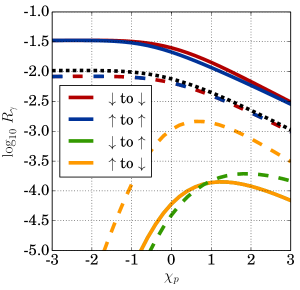
Figure 2: The rate of polarised single Compton scattering $R_{\gamma}$. The solid (dashed) lines refer to a photon scattered into the $\varepsilon_{k}^{(1)}$ ($\varepsilon_{k}^{(2)}$) polarisation state and the dotted line refers to the unpolarised rate.

III Double Compton scattering

Let us now turn to the calculation of double photon emission by an electron in a plane wave field. We are considering the process

$$e^{-}\to e^{-}+\gamma+\gamma^{\prime}$$ (17)

and the corresponding Feynman diagram is given in Fig. 3. The transition matrix element for this process is

$$S_{fi} = \overrightarrow{S_{fi}}+\overleftarrow{S_{fi}}$$ (18)

$$\overrightarrow{S_{fi}} = -e^{2}\int\!d^{4}x^{\prime}\,d^{4}x~{}\overline{\psi}_{p^{\prime}}(x^{\prime})\frac{\sqrt{4\pi}\not{\varepsilon}^{\prime\,\ast}_{k^{\prime}}}{\sqrt{2Vk^{\prime\,0}}}\mbox{e}^{ik^{\prime}x^{\prime}}G(x^{\prime},x)\mbox{e}^{ikx}\frac{\sqrt{4\pi}\not{\varepsilon}^{\ast}_{k}}{\sqrt{2Vk^{0}}}\psi_{p}(x),$$ (19)

$$G(x^{\prime},x) = \int\!\frac{d^{4}q}{(2\pi)^{4}}\left[1+\frac{e\not{\varkappa}\not{A}(\varphi^{\prime})}{2\,\varkappa\cdot q}\right]\mbox{e}^{iS(q,\varphi^{\prime})}\frac{\not{q}+m}{q^{2}-m^{2}+i0}\mbox{e}^{-iS(q,\varphi)}\left[1+\frac{e\not{A}(\varphi)\not{\varkappa}}{2\,\varkappa\cdot q}\right]$$ (20)

where $\overrightarrow{S_{fi}}$ corresponds to the first diagram in Fig. 3 and $\overleftarrow{S_{fi}}$ to making the replacements $k,\varepsilon_{k}\leftrightarrow k^{\prime},\varepsilon_{k^{\prime}}$.

Figure 3: The Feynman diagram for double Compton scattering. The prescription on the exchange term $\left(k\leftrightarrow k^{\prime}\right)$ also applies to swapping the polarisation vectors.

The method of calculation is similar to in the previous section, with the added complication of having an extra diagram due to bosonic exchange symmetry of identical outgoing photons as well as a fermionic propagator (a detailed example of the Nikishov-Ritus approach being applied to a two-vertex process is given in the calculation of electron-seeded pair creation in King and Ruhl (2013)). We will confine ourselves to calculating the unpolarised double Compton scattering probability $P_{\gamma\gamma}$

$$P_{\gamma\gamma}=\frac{1}{4}V^{3}\int\frac{d^{3}p^{\prime}}{(2\pi)^{3}}\,\frac{d^{3}k}{(2\pi)^{3}}\frac{d^{3}k^{\prime}}{(2\pi)^{3}}~{}\textrm{tr}\,|S_{fi}|^{2},$$ (21)

with the pre-factor including an average over initial electron spins and symmetry factor due to identical diagrams. The modulus squared amplitude contains each exchange term mod-squared plus interference terms

$$|S_{fi}|^{2}=|\overrightarrow{S_{fi}}|^{2}+|\overleftarrow{S_{fi}}|^{2}+\overleftarrow{S_{fi}}\overrightarrow{S_{fi}}^{\ast}+\overrightarrow{S_{fi}}\overleftarrow{S_{fi}}^{\ast}.$$ (22)

Now suppose the $p^{\prime}$ integral in Eq. (21) is performed by evaluating the standard total momentum-conserving delta function that arises in scattering matrix calculations and that the integral over $k$ and $k^{\prime}$ remain. In the standard fashion, these integrals can be re-interpreted as

$$\int d(k\cdot a^{(1)})\,d(k^{\prime}\cdot a^{(1)})\bigg{|}_{\textrm{on shell}}=\int\frac{d\varphi_{+}\,d\varphi_{-}}{J}.$$ (23)

Here, $\varphi_{+}=(\varphi_{x^{\prime}}+\varphi_{x})/2$ is the average of the stationary phases in the function describing the probability of photon emission at spacetime points $x$ and $x^{\prime}$ and hence corresponds to the centre in phase between two emissions and $\varphi_{-}=\varphi_{x^{\prime}}-\varphi_{x}>0$ is the phase the electron travels between emissions, where $J$ is the corresponding Jacobian. Part of the integrand is completely independent of both these phases, and we term this the two-step process, part of the integrand depends only on $\varphi_{-}$, and we term this the one-step process and the remaining part of the integrand depends on both phases. Since these phase integrations are formally infinite in a constant crossed field, the part that depends on both phases and gives a finite answer, will be dropped from the calculation. It can be shown King and Ruhl (2013) that this neglected part corresponds to the interference terms in Eq. (22). As the total probability includes an integration over both photon momenta, one can then replace $|S_{fi}|^{2}\to 2|\overrightarrow{S_{fi}}|^{2}$ in the integrand. If we again define the rate $R_{\gamma\gamma}=P_{\gamma\gamma}/\xi\int d\varphi_{+}$ where $\varphi=\varphi_{x}$ is the phase of the first emission the total rate becomes

$$R_{\gamma\gamma}=R^{(2)}_{\gamma\gamma}+R^{(1)}_{\gamma\gamma}$$ (24)

where the superscripts indicate the two- and one- step rates accordingly and

$$R^{(2)}_{\gamma\gamma} = \mathcal{I}^{(2)}_{\gamma\gamma}~{}\xi\int d\varphi_{-}$$ (25)

$$R^{(1)}_{\gamma\gamma} = \mathcal{I}^{(1)}_{\gamma\gamma},$$ (26)

where the quantities $\mathcal{I}_{\gamma\gamma}$ are free of divergences associated with the infinite expanse of the background and will be referred to as the dynamical part of the rate in contrast to the spacetime factors that multiply them in the probability, such as integrations over external-field phase.

III.1 Two-step double Compton scattering

The two-step process actually comprises terms from both the on- and off- shell part of the fermion propagator, where off-shell terms are essential to preserve causality King and Ruhl (2013), so it is not synonymous with the “on-shell” part. We find

$$\mathcal{I}_{\gamma\gamma}^{(2)} = -\alpha^{2}\int\!d\chi_{k}d\chi_{k^{\prime}}\,\left[C^{\cdot\cdot}\textrm{Ai}(z)\textrm{Ai}(z^{\prime})+\right.$$ (27)

$$\left.C^{\prime\prime}\textrm{Ai}^{\prime}(z)\textrm{Ai}^{\prime}(z^{\prime})+C^{\prime 1}\textrm{Ai}^{\prime}(z)\textrm{Ai}_{1}(z^{\prime})+\right.$$

$$\left.C^{1\prime}\textrm{Ai}_{1}(z)\textrm{Ai}^{\prime}(z^{\prime})+C^{11}\textrm{Ai}_{1}(z)\textrm{Ai}_{1}(z^{\prime})\right],$$

where we have defined

$$z = \left[\frac{\chi_{k}}{\chi_{p}\chi_{q}}\right]^{2/3},\quad z^{\prime}=\left[\frac{\chi_{k^{\prime}}}{\chi_{p^{\prime}}\chi_{q}}\right]^{2/3};$$ (28)

$$C^{\cdot\cdot} = -\frac{zz^{\prime}\chi_{p}\chi_{p^{\prime}}}{(\chi_{p}\chi_{q})^{2}}$$ (29)

$$C^{\prime\prime} = \frac{1}{(\chi_{p}\chi_{q})^{2}}\left(\frac{2}{z^{\prime}}+\chi_{k^{\prime}}z^{\prime\,1/2}\right)\left(\frac{2}{z}+\chi_{k}z^{1/2}\right)$$ (30)

$$C^{\prime 1} = \frac{1}{(\chi_{p}\chi_{q})^{2}}\left(\frac{2}{z}+\chi_{k}z^{1/2}\right)$$ (31)

$$C^{1\prime} = \frac{1}{(\chi_{p}\chi_{q})^{2}}\left(\frac{2}{z^{\prime}}+\chi_{k^{\prime}}z^{\prime\,1/2}\right)$$ (32)

$$C^{11} = \frac{1}{(\chi_{p}\chi_{q})^{2}},$$ (33)

with $\chi_{q}=\chi_{p}-\chi_{k}$ and $\chi_{p^{\prime}}=\chi_{p}-\chi_{k}-\chi_{k^{\prime}}$. Written in this way, upon comparison with the probability for unpolarised single photon scattering (averaging over photon polarisation and setting $\sigma_{p},\sigma_{q}\to 0$ in Eq. (LABEL:eqn:Cgs)), one can see that the two-step process is the integral over the product of single Compton scattering. We find that the unpolarised two-step rate can indeed be exactly factorised in terms of single Compton scattering processes, when the intermediate electron’s spin is taken into account and assumed in an unchanged state when the second photon is emitted (we note here the relevance of choosing a non-precessing spin basis)

$$R_{\gamma\gamma}^{(2)}=\frac{1}{2}\sum_{\sigma_{q}}\int d\chi_{q}\frac{\partial R_{\gamma}(\chi_{p})}{\partial\chi_{q}}\,R_{\gamma}(\chi_{q})\,\frac{\xi}{2}\int d\varphi_{-}.$$ (34)

III.2 One-step double Compton scattering

The one-step process involves an extra integration over a variable related to the virtuality of the propagating electron.

$$\mathcal{I}_{\gamma\gamma}^{(1)}=-\frac{\alpha^{2}}{4\pi}\int\!d\chi_{k}\,d\chi_{k^{\prime}}\,dt~{}\frac{\mathcal{A}(t)+\mathcal{A}(-t)-2\mathcal{A}(0)}{t^{2}}$$ (35)

$$\mathcal{A}(t) = C^{\cdot\cdot}_{t}\textrm{Ai}(z_{t})\textrm{Ai}(z_{t}^{\prime})+$$ (36)

$$C^{\prime\prime}_{t}\textrm{Ai}^{\prime}(z_{t})\textrm{Ai}^{\prime}(z_{t}^{\prime})+C^{\prime 1}_{t}\textrm{Ai}^{\prime}(z_{t})\textrm{Ai}_{1}(z_{t}^{\prime})+$$

$$C_{t}^{1\prime}\textrm{Ai}_{1}(z_{t})\textrm{Ai}^{\prime}(z^{\prime}_{t})+C^{11}_{t}\textrm{Ai}_{1}(z_{t})\textrm{Ai}_{1}(z^{\prime}_{t})$$

$$z_{t} = z+\frac{t}{z^{1/2}},\qquad z^{\prime}_{t}=z^{\prime}-\frac{t}{z^{\prime 1/2}},$$ (37)

where we have defined

$$\frac{C^{\cdot\cdot}_{t}}{C^{\cdot\cdot}} = 1-\frac{t}{2}\frac{\chi_{q}(\chi_{p}+\chi_{q})(\chi_{q}+\chi_{p^{\prime}})}{\chi_{k}\chi_{k^{\prime}}}$$ (38)

$$\frac{C^{\prime\prime}_{t}}{C^{\prime\prime}} = 1$$ (39)

$$\frac{C^{\prime 1}_{t}}{C^{\prime 1}} = 1+\frac{t\chi_{k}}{2}$$ (40)

$$\frac{C^{1\prime}_{t}}{C^{1\prime}} = 1-\frac{t\chi_{k^{\prime}}}{2}$$ (41)

$$\frac{C^{11}_{t}}{C^{11}} = 1+t\frac{\chi_{q}^{2}-\chi_{k}\chi_{k^{\prime}}}{2\chi_{q}}+\frac{t^{2}}{4}(\chi_{p}\chi_{p^{\prime}}-\chi_{k}\chi_{k^{\prime}}).$$ (42)

After performing the integral over the propagator variable $t$ and $\chi_{k^{\prime}}$, the remaining integral in $\chi_{k}$ diverges $\sim 1/\chi_{k}$ for $\chi_{k}\to 0$. This well-known infra-red divergence was reported in other calculations in double Compton scattering Lötstedt and Jentschura (2009a, b); Seipt and Kämpfer (2012), and should be cancelled when self-energy corrections are included Morozov and Ritus (1975).

It can be shown King and Ruhl (2013) that the one-step process can be written as a term originating from the interference between two- and one- step parts of the amplitude plus a term originating solely from the one-step part of the amplitude. Here, as in electron-seeded pair creation in a constant crossed field, parts of the one-step probability are negative, however since the phase factor multiplying the two-step term is formally divergent, the total probability is non-negative. Unlike for electron-seeded pair creation, we find no threshold value of $\chi_{p}$ above which the one-step process becomes positive.

IV Approximations used in simulation

We turn now to a comparison of the analytical results for double Compton scattering with approximations used in numerical simulations. In particular, we investigate two assumptions. First, the neglecting of electron spin, which we found essential to correctly factorising the two-step part of double Compton scattering and which produced new terms in the integrand. Second, the neglecting of the one-step process also known as “simultaneous” two-photon emission by an electron.

IV.1 Electron spin

As an example of employing the constant crossed field approximation, the unpolarised probability of the two-step process in a slowly-varying external field can be written as a double iteration of single photon emission:

$$P_{\textrm{ccf}}^{(2)}=\frac{1}{2}\sum_{\sigma_{q}}\int d\varphi_{\xi^{\prime}}d\varphi_{\xi}d\chi_{q}\,P_{\gamma}[\chi_{q}]\,\frac{\partial P_{\gamma}[\chi_{p},\chi_{q}]}{\partial\chi_{q}},$$ (43)

where we have allowed the external field to depend on the phase by defining $\varphi_{\xi}=\varphi\,\xi(\varphi)$, $\varphi_{\xi^{\prime}}=\varphi^{\prime}\,\xi(\varphi^{\prime})$ and $\varphi_{\xi^{\prime}}>\varphi_{\xi}$, $\chi_{p}=\chi_{p}(\varphi_{\xi})$, $\chi_{q}=\chi_{q}(\varphi_{\xi^{\prime}})$ and $\chi_{q}>\chi_{p}$. If the external field is taken to be exactly constant $\xi(\varphi)=\xi$, Eq. (43) leads back to Eq. (34). It is therefore consistent to only include single Compton scattering in a simulational approach, and allow for the process to occur multiple times, as is performed in numerical simulation. To investigate the importance of including electron spin, we plot the dynamical part of the two-step double Compton scattering $\mathcal{I}_{\gamma\gamma}^{(2)}$ using Eq. (34), as well as the case when the propagating electron is forced to be unpolarised by setting $\sigma_{q}\to 0$ in Eq. (34), which we label $\overline{\mathcal{I}}_{\gamma\gamma}^{(2)}$. For comparative purposes, we also plot Morozov and Ritus’ asymptotic limits for the two-step process by introducing the function

$$\mathcal{I}_{\textrm{MR}}^{(2)}(\chi_{p})=\left\{\begin{array}[]{cl}\frac{25\alpha^{2}}{12}&\chi_{p}<1\\ \frac{119\alpha^{2}}{270}\Gamma(\frac{1}{3})(\frac{3}{\chi_{p}})^{2/3}&\chi_{p}>1\end{array}\right.,$$ (44)

where $\chi_{p}<1$ ($\chi_{p}>1$) is the $\chi_{p}\ll 1$ ($\chi_{p}\gg 1$) asymptotic limit.

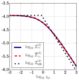
Figure 4: The dynamical part of the two-step probability $\mathcal{I}_{\gamma\gamma}^{(2)}$ with the approximation of using unpolarised electrons $\overline{\mathcal{I}}_{\gamma\gamma}^{(2)}$ and the asymptotic limits of Morozov and Ritus $\mathcal{I}^{(2)}_{\textrm{MR}}$

In Fig. 4, we note that the intermediate electron’s spin seems to make very little difference to the total probability for double Compton scattering. We highlight the property of Compton scattering in a constant crossed field, that $\partial P_{\gamma}/\partial\chi_{k}\sim\chi_{k}^{-2/3}$ for $\chi_{k}\to 0$. Although the differential probability diverges as $\chi_{k}\to 0$, the total probability remains finite (the softening of this well-known infra-red divergence has recently been studied in Lavelle and McMullan (2006); Dinu et al. (2012); Ilderton and Torgrimsson (2013)). How to take into account this divergent number of photons is handled in a variety of ways by numerical simulations, but often a hard energy or $\chi_{k}$ cutoff is introduced, below which the effects of the emitted radiation are included using the classical equations of electrodynamics. By introducing a cutoff in our analysis, for example, neglecting photons with $\chi_{k}<0.1$ (several orders of magnitude larger than what is usually considered Harvey et al. (2014)), the effect of the electron spin to the total probability is still only at the few percent level. Therefore, it seems that treating the propagating particle as a scalar in numerical simulations of multi-photon emission of electrons in intense laser pulses is a consistent approximation.

IV.2 Simultaneous photon emission

With simultaneous photon emission, we are referring to the one-step process given by the integral in Eq. (35). We have already commented that this is divergent and negative. Therefore comparison of the factorised two-step process with the “rest” of the probability of two-photon emission is not possible at $O(\alpha^{2})$ without including self-energy terms. Although it makes little sense to compare two- and one- step processes without including self-energy terms, as they may also appreciably affect photon emission for large $\chi$ values, we can assess how much of the one-step process is neglected in simulation codes when a cutoff in the emitted photons’ $\chi$ parameter is used. For example, in the simulation of photon emission by a single electron in Harvey et al. (2014), a cutoff of $\chi_{k}=\Delta_{k}=10^{-5}$ was chosen. In Fig. 5 we compare the total probability of the one- and two- step processes using $\chi_{k}$ and $\chi_{k^{\prime}}$ cutoffs of $\Delta_{k}=\Delta_{k^{\prime}}=\Delta=10^{-5}$.

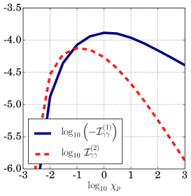
Figure 5: The absolute dynamical part of the one-step probability $\mathcal{I}_{\gamma\gamma}^{(1)}$ is compared to the two-step probability $\mathcal{I}_{\gamma\gamma}^{(2)}$ including an infra-red cutoff $\Delta_{k}=\Delta_{k^{\prime}}=10^{-5}$.

For $\chi_{p}\gg 1$, $\mathcal{I}_{\gamma\gamma}^{(1)}$ agrees with the scaling and sign given by Morozov and Ritus for this limit, although we were unable to compare results in a quantitative way. We note that the absolute ratio of dynamical parts of the one- to the two- step probabilities becomes larger than unity already at $\chi_{p}\approx 0.1$, and linearly increases to more than an order of magnitude for $\chi_{p}\gtrsim 50$. After repeating the calculation for a range of cutoffs $\Delta\in[10^{-7},10^{-2}]$, although the exact ratio is weakly cutoff-dependent, for $\chi_{p}\in[1,1000]$, the linear increase in the ratio appears cutoff-independent.

Over the formation length $1/\xi\varkappa^{0}$ the one-step process can clearly be dominant compared to the two-step process, which implies current numerical approaches are inappropriate for simulating double photon emission in this parameter regime. We recall the total rate for two-photon emission in a constant crossed field is given by

$$R_{\gamma\gamma}=\mathcal{I}^{(2)}_{\gamma\gamma}~{}\frac{\xi}{2}\int d\varphi_{-}+\mathcal{I}^{(1)}_{\gamma\gamma}+\frac{\mathcal{I}^{(0)}_{\gamma\gamma}}{\xi\int d\varphi_{-}},$$ (45)

where $\mathcal{I}^{(0)}_{\gamma\gamma}$ is the interference between exchange terms, neglected as the phase factor is formally infinite, but reintroduced here when discussing approximating more complicated fields as constant crossed. The constant crossed approximation to an arbitrary field is expected to be valid when $\xi\gg 1$ and $\chi_{p}$ is much larger than the two electromagnetic invariants $e^{2}F^{2}/m^{4}$ and $e^{2}FF^{\ast}/m^{4}$ for Faraday tensor $F$ and its dual $F^{\ast}$ Ritus (1985). The present results imply that the further assumption made in simulations that the rate of generating $n$ photons is due to the $n$-step process, is questionable for $n=2$ when $\xi\lesssim O(10^{2})$ and $\chi_{p}\gtrsim 1$. To demonstrate this, we use the constant crossed field approximation in Eq. (43) and

$$P^{(1)}_{\textrm{ccf}}=\int\!d\varphi_{\xi}\,R_{\gamma\gamma}^{(1)}[\chi_{p}(\varphi_{\xi})]$$ (46)

to estimate double Compton scattering in the field of a laser pulse $E=E_{0}\,\cos^{4}(\pi\varphi/2\Phi)\cos\varphi$ for pulse width $\Phi=\varkappa^{0}\tau$.

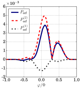
Figure 6: For a few-cycle pulse with field strength equivalent to $500\,\textrm{TeV}$ focussed to a focal width of $10\,\mu\textrm{m}$ of $910\,\textrm{nm}$ wavelength with peak $\xi=10$, and pulse duration $5\,\textrm{fs}$ counterpropagating with $10\,\textrm{GeV}$ seed electrons.

In Fig. 6, the relative difference in photon yield due to including the one-step process is $-25\%$, however the main qualitative difference due to including the one-step process is the instant when two-photon emission starts to become significant, which is predicted to occur a half-cycle later.

Although we have seen that one requires background fields less than two orders of magnitude larger than the formation length $1/\xi\varkappa^{0}$ and $\chi_{p}\gg 0.1$ for the one-step process to be comparable to the two-step one, the analysis raises the question of how accurate it is to simulate an $n$-photon emission including just the $n$-step process.

V Conclusion

Using a non-precessing spin basis to describe electron polarisation, the probability of a spin flip following single Compton scattering in a constant crossed field was found to be suppressed. The unpolarised rate for double Compton scattering in a constant crossed field was written as a sum of a two-step process, which is exactly factorisable as single Compton scattering integrated over the longitudinal momentum of a polarised intermediate electron, and a one-step process, which dominates the total probability over the formation length $1/\xi\varkappa^{0}=\lambdabar E_{\textrm{cr}}/E$. Regarding numerical simulation of double photon emission, we found the assumption that the intermediate electron is unpolarised, to be accurate to the few percent level, depending on the photon energy cutoff used and that although simultaneous two-photon emission can be much more probable than sequential emission, when the external field’s spatial dimensions are more than around two orders of magnitude larger than the single-photon formation length, the sequential process is dominant. The availability of intense ultra-short laser pulses would allow measurement of the quantum interference between simultaneous and sequential production channels in the nonlinear domain.

VI Acknowledgments

B.K. acknowledges the stimulating and enlightening discussions with A. Fedotov and M. Legkov that inspired this project and conversations on the infra-red with M. Lavelle and A. Ilderton. This work was in part supported by the Russian Fund for Basic Research, grant No.13-02-90912.

References

- Jackson (1975) J. D. Jackson, Classical Electrodynamics (John Wiley & Sons, Inc., New York, 1975).
- Nikishov and Ritus (1964) A. I. Nikishov and V. I. Ritus, Sov. Phys. JETP 19, 529 (1964).
- Brown and Kibble (1964) L. S. Brown and T. W. B. Kibble, Phys. Rep. 133, A705 (1964).
- Narozhny and Fofanov (1996) N. B. Narozhny and M. S. Fofanov, Sov. Phys. JETP 83, 14 (1996).
- Boca and Florescu (2009) M. Boca and V. Florescu, Phys. Rev. A 80, 053403 (2009), URL http://link.aps.org/doi/10.1103/PhysRevA.80.053403.
- Harvey et al. (2009) C. Harvey, T. Heinzl, and A. Ilderton, Phys. Rev. A 79, 063407 (2009).
- Mackenroth et al. (2010) F. Mackenroth, A. Di Piazza, and C. H. Keitel, Phys. Rev. Lett. 105, 063903 (2010), URL http://link.aps.org/doi/10.1103/PhysRevLett.105.063903.
- Heinzl et al. (2010) T. Heinzl, A. Ilderton, and M. Marklund, Phys. Lett. B 692, 250 (2010).
- Mackenroth and Di Piazza (2011) F. Mackenroth and A. Di Piazza, Phys. Rev. A 83, 032106 (2011), URL http://link.aps.org/doi/10.1103/PhysRevA.83.032106.
- Krajewska and Kamiński (2013) K. Krajewska and J. Z. Kamiński, Laser and Particle Beams 31, 503 (2013).
- King et al. (2013) B. King, N. Elkina, and H. Ruhl, Phys. Rev. A 87, 042117 (2013).
- Ivanov et al. (2004) D. Ivanov, G. Kotkin, and V. Serbo, Eur. Phys. J. C 36, 127 (2004), ISSN 1434-6044, URL http://dx.doi.org/10.1140/epjc/s2004-01861-x.
- Bashmakov et al. (2014) V. F. Bashmakov, E. N. Nerush, I. Y. Kostyukov, A. M. Fedotov, and N. B. Narozhny, Phys. Plasmas 21 (2014).
- Bula et al. (1996) C. Bula et al., Phys. Rev. Lett. 76, 3116 (1996), URL http://link.aps.org/doi/10.1103/PhysRevLett.76.3116.
- Bamber et al. (1999) C. Bamber et al., Phys. Rev. D 60, 092004 (1999).
- Seipt and Kämpfer (2012) D. Seipt and B. Kämpfer, Phys. Rev. D 85, 101701 (2012).
- Mackenroth and Di Piazza (2013) F. Mackenroth and A. Di Piazza, Phys. Rev. Lett. 110, 070402 (2013).
- Ritus (1985) V. I. Ritus, J. Russ. Laser Res. 6, 497 (1985).
- Marklund and Shukla (2006) M. Marklund and P. K. Shukla, Rev. Mod. Phys. 78, 591 (2006).
- Di Piazza et al. (2012) A. Di Piazza et al., Rev. Mod. Phys. 84, 1177 (2012).
- Sokolov et al. (2010) I. V. Sokolov et al., Phys. Rev. Lett. 105, 195005 (2010).
- Nerush et al. (2011) E. N. Nerush et al., Phys. Rev. Lett. 106, 035001 (2011).
- Elkina et al. (2011) N. V. Elkina et al., Phys. Rev. ST Accel. Beams 14, 054401 (2011).
- Blackburn et al. (2014) T. G. Blackburn, C. P. Ridgers, J. G. Kirk, and A. R. Bell, Phys. Rev. Lett. 112, 015001 (2014), URL http://link.aps.org/doi/10.1103/PhysRevLett.112.015001.
- Green and Harvey (2014) D. G. Green and C. N. Harvey, Phys. Rev. Lett. 112, 164801 (2014), URL http://link.aps.org/doi/10.1103/PhysRevLett.112.164801.
- Green and Harvey (2014) D. G. Green and C. N. Harvey, arXiv:1410.4055 (2014).
- Mironov et al. (2014) A. A. Mironov, N. B. Narozhny, and A. A. Fedotov, arXiv:1407.6760 (2014).
- Morozov and Ritus (1975) D. A. Morozov and V. I. Ritus, Nucl. Phys. B 86, 309 (1975).
- Mandl and Shaw (2010) F. Mandl and G. Shaw, Quantum Field Theory (John Wiley & Sons (second edition), 2010).
- Volkov (1935) D. M. Volkov, Z. Phys. 94, 250 (1935).
- Berestetskii et al. (1982) V. B. Berestetskii, E. M. Lifshitz, and L. P. Pitaevskii, Quantum Electrodynamics (second edition) (Butterworth-Heinemann, Oxford, 1982).
- Dinu et al. (2014a) V. Dinu, T. Heinzl, A. Ilderton, M. Marklund, and G. Torgrimsson, Phys. Rev. D 89, 125003 (2014a), URL http://link.aps.org/doi/10.1103/PhysRevD.89.125003.
- Dinu et al. (2014b) V. Dinu, T. Heinzl, A. Ilderton, M. Marklund, and G. Torgrimsson, Phys. Rev. D 90, 045025 (2014b), URL http://link.aps.org/doi/10.1103/PhysRevD.90.045025.
- King et al. (2010) B. King, A. Di Piazza, and C. H. Keitel, Phys. Rev. A 82, 032114 (2010).
- King et al. (2014) B. King, P. Böhl, and H. Ruhl, Phys. Rev. D 90, 065018 (2014), URL http://link.aps.org/doi/10.1103/PhysRevD.90.065018.
- Bargmann et al. (1959) V. Bargmann, L. Michel, and V. L. Telegdi, Phys. Rev. Lett. 2, 435 (1959).
- Odom et al. (2006) B. Odom et al., Phys. Rev. Lett. 97, 030801 (2006).
- Gabrielse et al. (2007) G. Gabrielse et al., Phys. Rev. Lett. 99, 039902 (2007).
- Heinzl and Ilderton (2009) T. Heinzl and A. Ilderton, Opt. Commun. 282, 1879 (2009).
- King and Ruhl (2013) B. King and H. Ruhl, Physical Review D 88, 013005 (2013).
- Lötstedt and Jentschura (2009a) E. Lötstedt and U. D. Jentschura, Phys. Rev. Lett. 103, 110404 (2009a).
- Lötstedt and Jentschura (2009b) E. Lötstedt and U. D. Jentschura, Phys. Rev. A 80, 053419 (2009b).
- Lavelle and McMullan (2006) M. Lavelle and D. McMullan, JHEP 03, 026 (2006).
- Dinu et al. (2012) V. Dinu, T. Heinzl, and A. Ilderton, Phys. Rev. D 86, 085037 (2012), URL http://link.aps.org/doi/10.1103/PhysRevD.86.085037.
- Ilderton and Torgrimsson (2013) A. Ilderton and G. Torgrimsson, Phys. Rev. D 87, 085040 (2013), URL http://link.aps.org/doi/10.1103/PhysRevD.87.085040.
- Harvey et al. (2014) C. Harvey, A. Ilderton, and B. King, arXiv:1409.6187 (2014).