Recognizing molecular patterns by machine learning:
an agnostic structural definition of the hydrogen bond.

Abstract

The concept of chemical bonding can ultimately be seen as a rationalization of the recurring structural patterns observed in molecules and solids. Chemical intuition is nothing but the ability to recognize and predict such patterns, and how they transform into one another. Here we discuss how to use a computer to identify atomic patterns automatically, so as to provide an algorithmic definition of a bond based solely on structural information. We concentrate in particular on hydrogen bonding – a central concept to our understanding of the physical chemistry of water, biological systems and many technologically important materials. Since the hydrogen bond is a somewhat fuzzy entity that covers a broad range of energies and distances, many different criteria have been proposed and used over the years, based either on sophisticate electronic structure calculations followed by an energy decomposition analysis, or on somewhat arbitrary choices of a range of structural parameters that is deemed to correspond to a hydrogen-bonded configuration. We introduce here a definition that is univocal, unbiased, and adaptive, based on our machine-learning analysis of an atomistic simulation. The strategy we propose could be easily adapted to similar scenarios, where one has to recognize or classify structural patterns in a material or chemical compound.

Introduction

Modern chemistry can be regarded as the (very successful) effort of rationalizing the stability and reactivity of compounds in terms of chemical bonding.Pauling (1960) A theory that aims at predicting the structure and formation of chemical bonds from first principles cannot disregard a more or less explicit quantum mechanical description of electrons. However, from a purely heuristic point of view, one could also interpret the recurrence of structural patterns, in terms of distances and angles between atomic nuclei, as a sign of the underlying chemical bond. In fact, chemical intuition builds on the possibility of recognizing these patterns and predicting whether and how they can be modified during a chemical reaction.

Electronic structure methods – from density-functional theory (DFT) and Hartree-Fock to more accurate and demanding quantum chemistry approaches – make it possible to predict with great accuracy the structure and the stability of a molecule or a material from first principles,Car and Parrinello (1985); Schaefer III (2012) and empirical force fields have been parametrized to reproduce these results at a fraction of the cost.MacKerell et al. (1998); Behler and Parrinello (2007); Bartók et al. (2010) A computer simulation based on these techniques makes it possible to observe atomic configurations that are consistent with their energetic stability and the thermodynamic conditions, so in many cases the problem one faces in computational modeling is not so much to predict recurring structural patterns, as to recognize them in a clear, unbiased way.

An excellent example of this kind of scenario is that of recognizing hydrogen bonds. Since it was made popular by Pauling,Pauling (1928) the concept of hydrogen bond has been a cornerstone in our understanding of water, biological systems and supramolecular aggregates.Pauling et al. (1951); Guo and Karplus (1994); Jeffrey (1997) Spanning a range of bond energies going from almost covalent bonds to Van Der Waals interactions, hydrogen bonds can form and break easily at room temperature, explaining their importance for biological processes.Desiraju and Steiner (2001) While in most cases the hydrogen bond can be understood as an electrostatic effect – and simple empirical models based on point charges are capable of qualitatively reproducing the structure and energetics obtained with electronic structure methods – there are also examples in which one can recognize a strongly covalent character, which is often associated with quantum delocalization of the proton along the bond.Lin et al. (2011); McKenzie et al. (2014) Because of their flexibility, hydrogen bonds escape an obvious, universal description, and several definitions exist based on somewhat arbitrary ranges of structural parametersWeinhold and Klein (2012) and/or decompositions of the total energy obtained from electronic structure calculations.Wendler et al. (2010); Azar and Head-Gordon (2012); Weinhold and Klein (2014); Kühne and Khaliullin (2014)

This paper aims at introducing a general protocol to automatically analyze the outcome of an atomistic simulation, in order to recognize recurring structural patterns in a quantitative, deterministic and unbiased way. Starting from a (possibly) high-dimensional description of groups of atoms, for instance the set of inter-atomic distances, we propose to infer a Gaussian mixture model for the probability distribution of these initial coordinates. In order to obtain a deterministic, parameter-less partitioning of the probability density it is best to first apply a mode-seeking algorithmVedaldi and Soatto (2008) to perform a non-parametric clustering, and then to find the best Gaussian fit to each mode of the distribution. One (or more) of the clusters can then be traced to the structural pattern(s) of interest. What is more, this approach gives a natural out-of-sample probabilistic definition of a structural pattern, that can be used to identify the same patterns in new configurations of the system.

We dub this algorithm PAMM (probabilistic analysis of molecular motifs), and describe in detail its rationale, functioning and implementation in Section I. We will then focus on the hydrogen bond as an instructive and challenging benchmark of our procedure, present several different examples in Section II, and finally give our conclusions.

I A probabilistic analysis of molecular motifs

The approach we introduce aims at using machine-learning algorithms to assist the interpretation of a computer experiment, and its rationalization in terms of recurring structural patterns and different forms of chemical bonding, automatically extracting information from the large data sets that are produced by atomistic simulations. We focus on using exclusively structural information to guide the analysis, partly because this is just more convenient than performing an energy decomposition analysis on top of an electronic structure calculation, partly because the (free) energetic stability of different molecular patterns is implicit in the frequency with which they appear in the simulation. We will formulate the discussion of the algorithm in very general terms, but use as a concrete example the case of the hydrogen bond in water, that we will discuss in more detail in Section II.

The analysis we propose is based on a preliminary atomistic simulation that produces configurations consistent with the energetics of the system of interest, and consists in three consecutive steps:

1. Definition of the training set: after having performed a reference simulation, one has to introduce a (possibly high-dimensional) description of the groups of atoms that might be involved in recurring molecular patterns. This step yields a set $\mathcal{X}=\left\{\mathbf{x}_{i}\right\}$ that contains $N$ vectors of dimensionality $D$, that represent molecular configurations observed in the simulation. A kernel density estimation is then used to evaluate the probability density that underlies the distribution of $\mathcal{X}$.

2. Determination of the mixture model: the probability density of $\mathcal{X}$ is analyzed to recognize the different modes of the distribution, and to partition $\mathcal{X}$ in $n$ disjoint clusters using the quick-shift algorithm Vedaldi and Soatto (2008). These clusters are then used to build a Gaussian mixture model, giving a probabilistic framework to associate regions of the $D$-dimensional space to one or more recurring patterns.

3. Analysis of the simulation: the mixture model can then be used to give qualitative and quantitative insight on the system being studied, and possibly as the basis for defining more complex orders parameters to describe and bias collective rearrangements of the various molecular patterns.

A simple library to apply PAMM to an arbitrary data set, and in the specific case of hydrogen-bond recognition is briefly discussed in Appendix A, and provided as open-source code in the Supplementary Materials (SM)si .

Figure 1: Simplified representation of the application of PAMM to a simple two-dimensional dataset. (a) A series of data points giving a (possibly high-dimensional) description of molecular patterns is taken as the input. (b) A sparse grid of points is selected by a minmax algorithm, and a kernel-density estimation of the probability distribution is evaluated at each point. (c) A quick-shift procedure is performed to assign each of the grid points to one of the modes of the probability distribution. (d) Clusters are determined based on the assignment to probability maxima. (e) A Gaussian mixture model is built by fitting separately a Gaussian to each cluster. (f) The posterior probabilities of the Gaussian mixture model provide a natural, fuzzy definition of regions of parameter space that define recurring molecular patterns.

Definition of the training set

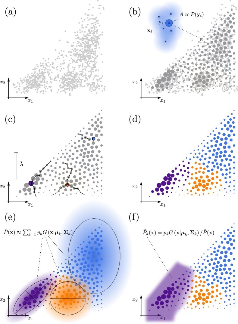
The analysis we propose starts by introducing descriptors of the relative arrangement of groups of atoms, for which one wishes to identify recurring patterns. If one wanted to recognize the existence of a bond between two atomic species, for instance, one could process the configurations from an atomistic simulation to output the list of distances between the pairs of atoms of the two species. For more complex structural patterns, one could pick all the possible tuples of atoms of a few selected species, and describe them in terms of all the pair-wise distances among them, possibly sorting groups of distances to account for the permutation of identical atoms Gallet and Pietrucci (2013). In general, one would obtain a list of $N$, $D$-dimensional vectors $\mathcal{X}=\left\{\mathbf{x}_{i}\right\}$ (Figure 1(a)) that contains the descriptors for all of the tuples of selected atom kinds that are found in the simulation .

For example, a putative hydrogen bond in water involves one hydrogen atom H and a donor oxygen atom O and an acceptor O^′. The three distances between these atoms suffice to determine completely the geometry of the group. The training data set $\mathcal{X}$ could then be composed of 3-dimensional vectors $x_{i}=\left(\nu=d(\text{O}_{i}-\text{H}_{i})-d(\text{O}^{\prime}_{i}-\text{H}_{i}),\right.$ $\mu=d(\text{O}_{i}-\text{H}_{i})+d(\text{O}^{\prime}_{i}-\text{H}_{i}),$ $\left.r=d(\text{O}_{i}-\text{O}^{\prime}_{i})\right)$, each describing the configuration of a triplet of atoms that could possibly form a hydrogen bond.

One can then use the data set $\mathcal{X}$ to evaluate an estimate of the underlying probability distribution $P\left(\mathbf{x}\right)$. Since the $N$ points are distributed irregularly, and the possibly very high dimensionality of the data set makes it impractical to define the probability density on a regular grid, we used kernel density estimation (KDE) Silverman (1986) to compute an estimate of $P\left(\mathbf{x}\right)$.

For computational efficiency, we first selected a sub-set of the data samples $\mathcal{Y}\subseteq\mathcal{X}$ using a minmax criterion.Eldar et al. (1997) We chose a first point $\mathbf{y}_{1}\in\mathcal{X}$ at random, and then iterated

$$\mathbf{y}_{j+1}=\operatorname*{arg\,max}_{\mathbf{y}\in\mathcal{X}}\left[\min_{i\leq j}\left|\mathbf{y}_{i}-\mathbf{y}\right|\right].$$ (1)

Each new point is the sample with the maximal minimum distance to the points that had already been selected. The procedure was repeated until $M$ points had been chosen, forming a sparse grid on which the probability is to be estimated (Figure 1(b)). We found that $M=\sqrt{N}$ gives a good compromise between the density of the $\mathcal{Y}$ grid and the computational cost of the procedure (see the supplementary information for a discussion of the sensitivity of the method to this and other parameters).

The kernel density estimate on each grid point is defined as

$$P(\mathbf{y}_{i})=\sum_{j=1}^{N}w_{j}K\left(\left|\mathbf{x}_{j}-\mathbf{y}_{i}\right|,\sigma_{j}\right)/\sum_{j=1}^{N}w_{j},$$ (2)

where we used a Gaussian kernel

$$K(x,\sigma)=\left(2\pi\sigma^{2}\right)^{-D/2}e^{-\frac{x^{2}}{2\sigma^{2}}}$$ (3)

and we introduced for each sample a weight $w_{j}$ and an adaptive kernel width $\sigma_{j}$. The weights can be for instance defined to compensate for the trivial dependence of the probability density on the phase space volume due to the definition of the tuples, i.e. $w_{j}=w(\mathbf{x}_{j})$, where the weight function is defined so that a random distribution of atoms would give a constant $P(\mathbf{x})$.

The method does not depend dramatically on the choice of the kernel width, but we found it convenient to define automatically an adaptive width as follows. For each of the grid points we evaluated the minimum distance of the surrounding grid points, $\delta_{i}=\min_{j\neq i}\left|\mathbf{y}_{j}-\mathbf{y}_{i}\right|$. We then associated each of the sample points $\mathbf{x}_{j}$ to the nearest grid point $\mathbf{y}_{i}$, and set $\sigma_{j}=\delta_{i}$. Associating each sample point to the nearest grid point is also useful to speed up the evaluation of Eq. (2), as one can restrict the evaluation of the density kernel to points that are associated with the grid sites within a reasonable cut-off distance.

Determination of the mixture model

Having computed the kernel density estimation of $P(\mathbf{y}_{i})$, we could then proceed to subdivide it in distinct clusters, that will be associated to one or more recurring molecular patterns.

In order to fulfill our goal of having a univocal, deterministic pattern recognition, we opted for a non-parametric clustering of $P(\mathbf{x})$ based on mean shift Comaniciu and Meer (2002), a method that identifies the modes of the probability distribution and subdivides sample points by following steepest ascent paths starting from each point and clustering together the paths that converge onto the same local probability maximum. This approach has a profound physical interpretation: each probability maximum corresponds to a minimum in the free energy associated with the $D$-dimensional description of the group of atoms. Each of the clusters then corresponds to a meta-stable configuration.

For this application, we found that the most efficient and stable variant of the mean shift idea was the quick shift algorithm Vedaldi and Soatto (2008). Given a set of data points and an estimate of the density at each point ($\mathbf{y}_{i}$ and $P(\mathbf{y}_{i})$ in our case), quick shift builds a tree in which each data point is a node, and the root is the point with the highest density. Starting from each point, one connects it to the nearest point that has larger probability density, i.e. $\mathbf{y}_{i}$ is connected with the $\mathbf{y}_{j}$ such that

$$j=\operatorname*{arg\,min}_{P(\mathbf{y}_{j})>P(\mathbf{y}_{i})}\left|\mathbf{y}_{i}-\mathbf{y}_{j}\right|$$ (4)

The procedure defined by Eq. (4) will always end at the grid point with the highest associated probability density. In order to obtain individual modes of $P(\mathbf{x})$, one can introduce a length scale $\lambda$, and stop moving to points with higher $P$ whenever one cannot find one within $\lambda$ of the current point.. By setting a cutoff for the step length, quick shift identifies a set of $n$ local maxima $\mathbf{z}_{k}$, and partitions $\mathcal{Y}$ into $n$ disjoint sets $\mathcal{Z}_{k}$ based on the maximum to which a quick shift procedure started at each $\mathbf{y}_{i}$ converges to (Figure 1(c) and (d)).

One could then use the sets $\mathcal{Z}_{k}$ to define a non-parametric estimate of the cluster probabilities. We decided however to use them to define a Gaussian mixture model in which each cluster corresponds to one of the sets. Gaussian mixture modelsPress (2007); Reynolds (2009) are a particularly convenient approach to parametrically fit the probability distribution as a sum of $n$ multivariate Gaussians,

$$\hat{P}(\mathbf{x})=\sum_{k=1}^{n}p_{k}G\left(\mathbf{x}\middle|\bm{\mu}_{k},\bm{\Sigma}_{k}\right),$$ (5)

where $p_{k}$ is the fraction of density belonging to the $k$-th Gaussian (the relative weight of the cluster), $\bm{\Sigma}_{k}$ is its covariance matrix and $\bm{\mu}_{k}$ the mean:

$$G\left(\mathbf{x}\middle|\bm{\mu},\bm{\Sigma}\right)=\frac{1}{\sqrt{(2\pi)^{D}\det\bm{\Sigma}}}e^{{-\left(\mathbf{x}-\bm{\mu}\right)^{T}\bm{\Sigma}^{-1}\left(\mathbf{x}-\bm{\mu}\right)}/{2}}.$$ (6)

Fitting a parametric model such as (5) to the probability density lends itself quite naturally to a probabilistic interpretation in which each Gaussian function corresponds to a cluster, so that one can evaluate the probability that a point $\mathbf{x}$ belongs to the $k$-th cluster as

$$\hat{P}_{k}(\mathbf{x})=p_{k}G\left(\mathbf{x}\middle|\bm{\mu}_{k},\bm{\Sigma}_{k}\right)/\hat{P}(\mathbf{x}).$$ (7)

In the context of the present work, if we associate one of the Gaussian clusters of the density of sample points with the configuration pattern that we are trying to recognize, this cluster probability provides a very natural, fuzzy definition of the region of parameter space associated with the recurring pattern. $\hat{P}_{k}(\mathbf{x})$ varies smoothly between zero (configurations that clearly differ from the tagged cluster) to one (configurations that are undoubtedly to be assigned to the cluster), with intermediate values representing the “gray zone” at the margins of the cluster. For instance, as we shall see in Section II, if one can assign the $k$-th mode of $P(\nu,\mu,r)$ to hydrogen-bonded configurations, $\hat{P}_{k}(\nu,\mu,r)$ would give a data-driven hydrogen-bond count function, that would have a smooth transition between a value of 0 for non-hydrogen-bond configurations to 1 for configurations that clearly belong to the HB region of parameter space.

It is customary to train Gaussian mixture models by fitting the parameters $p_{k}$, $\bm{\mu}_{k}$, $\bm{\Sigma}_{k}$ so as to maximize the log-likelihood of the model given the underlying density $P(\mathbf{y}_{i})$,

$$\mathcal{L}=\sum_{i}P(\mathbf{y}_{i})\ln\hat{P}(\mathbf{y}_{i}).$$ (8)

This idea has been exploited before in the context of atomistic simulations, see e.g. Refs. Maragakis et al. (2009); Tribello et al. (2010); Pisani et al. (2014). We found however this procedure to be unreliable for our purposes: the optimized parameters depend dramatically on the number of clusters included in the model and on the initial values assigned to the parameters. Furthermore, if the modes of the probability distribution are not well described by Gaussians, it is often the case that more than one Gaussian is needed to describe each cluster, requiring further fine-tuning of the model.

To avoid this ambiguity, we did not obtain the Gaussian parameters by optimizing the log-likelihood of the model, but rather took one Gaussian for each of the clusters identified by quick shift, setting its mean at the maximum of the probability distribution and its covariance based on the distribution of the cluster members $\mathcal{Z}_{k}$ (Figure 1(e)):

$$\begin{split}\bm{\mu}_{k}=\mathbf{z}_{k},\quad p_{k}=\sum_{\mathbf{y}\in\mathcal{Z}_{k}}P(\mathbf{y})/\sum_{\mathbf{y}\in\mathcal{Y}}P(\mathbf{y}),\\ \bm{\Sigma}_{k}={\sum_{\mathbf{y}\in\mathcal{Z}_{k}}P(\mathbf{y})\left(\mathbf{y}-\mathbf{z}_{k}\right)\left(\mathbf{y}-\mathbf{z}_{k}\right)^{T}}/{\sum_{\mathbf{y}\in\mathcal{Z}_{k}}P(\mathbf{y})}.\end{split}$$ (9)

This choice combines the simplicity of a Gaussian mixture model, the fuzzy, smooth nature of the cluster probabilities (7), and the robust, deterministic partitioning of the probability density obtained with quick shift.

Analysis of the simulation

A critical analysis of the outcome of the quick shift partitioning of the probability density makes it possible to associate each cluster with a structural pattern, as described by the $D$ dimensional vector introduced in the first phase of our procedure. In many cases – such as the example of the hydrogen bond that we will discuss further below – one cluster stands out clearly as the distinct structural feature one is interested in, and one can focus further analysis on a single mode using the associated conditional probability function (7). For simplicity we will consider the selected cluster to be the one labeled by $k=1$.

The most direct application of the definition embodied by $\hat{P}_{1}(\mathbf{x})$ is to use it to test whether tuples of atoms $\mathbf{R}_{ijk\ldots}=(\mathbf{r}_{i},\mathbf{r}_{j},\mathbf{r}_{k},\ldots)$ match the definition of the structural pattern by computing

$$s^{(D)}_{ijk\ldots}=\hat{P}_{1}(\mathbf{x}(\mathbf{R}_{ijk\ldots})).$$ (10)

If the components of $\mathbf{x}$ are continuous functions of the atomic coordinates, $\hat{P}_{1}$ is a smooth continuous function too, that takes a value close to 1 whenever a group of atoms matches the target pattern (Figure 1(f)). This makes our definition of a pattern recognition function well-suited for use as a collective variable in accelerated sampling methods,Laio and Parrinello (2002) possibly in conjunction with other machine learning techniques to characterize the overall connectivity induced by the selected molecular pattern Pietrucci and Andreoni (2011), or similar fingerprint metrics that are guaranteed to distinguish dissimilar structures Sadeghi and Ghasemi (2013). The PAMM variables corresponding to different structural descriptor can also be analyzed to yield a coarse-grained, low-dimensional map Ferguson et al. (2010); Tribello et al. (2012); Rohrdanz et al. (2013). If necessary, one can artificially “soften” the transition between clusters, by dividing all the covariance matrices $\bm{\Sigma}_{k}$ in the Gaussian model by a scaling factor $\alpha$.

Since the $s^{(D)}_{ijk\ldots}$’s effectively count the instances of the structural pattern that are present at any given time in the trajectory, one can also combine several of these indicators together to count the number of patterns that involve a tagged atom $i$, or pair of atoms $\left(i,j\right)$:

$$s^{(1)}_{i}=\sum_{j,k,\ldots}s^{(D)}_{ijk\ldots},\quad s^{(2)}_{ij}=\sum_{k,\ldots}s^{(D)}_{ijk\ldots},\quad\text{etc.}$$ (11)

Depending on the application being considered, $s^{(1)}_{i}$ can be taken to represent the total coordination of the atom $i$, $s^{(2)}_{ij}$ the overall bonding between atoms $i$ and an atom $j$, and so on. For instance, by summing over all the possible acceptor atoms O^′ and hydrogen atoms H, one can get a smooth count of the total number of HBs donated by a selected oxygen O.

II The hydrogen bond, revisited

The PAMM framework we have introduced in the previous section is very abstract, and can be applied to any situation in which one wishes to recognize recurring motifs in an atomistic simulation. To demonstrate its application in a practical case, we chose to focus on recognizing the hydrogen bond (HB) in a number of different contexts. The term “hydrogen bond” refers to a highly directional three-centers interaction between two polar atoms and a hydrogen.Desiraju (2011); Arunan et al. (2011) The hydrogen atom H is covalently bound to one of the polar atoms, which is designated as the donor D, and points towards the second polar atom which is designated as the HB acceptor A. Despite the apparent simplicity of the concept, it is not easy to develop an universal definition of the HB, mostly because this entity has been used in many different contexts. The term has been associated to near-covalent interactions with an energy in excess of 30 kcal/mol, as well as to exceedingly weak ones with an energy of less than one kcal/mol. Typically hydrogen bonds are understood to have a predominantly electrostatic nature, with strongly electronegative donors and acceptors such as F, O or N. However, the observation of recurring C–H$\cdots$O units in the secondary structure of polypeptides have also been interpreted in terms of weak HBs, that have been suggested to play a significant role in stabilizing proteins.Derewenda et al. (1995)

Adding to the complexity of the broad energy scale covered by HBs is the fact that in most situations of interest thermal fluctuations and the environment modulate their stability, and that they are formed and destroyed on a relatively short time scale. One sees the difficulty in giving a clear-cut definition of a chemical entity which exhibits such a variability. The most generally applicable definitions rely on performing an electronic structure calculation, and on decomposing the energy of the systems in a sum of terms that can be interpreted as the binding energy of putative HBs.Reed et al. (1988); Pendás et al. (2006); Azar and Head-Gordon (2012); Kühne and Khaliullin (2014) Definitions that are based solely on structural information are much more practical, in that they do not require a supporting electronic structure calculation and can be applied to experimental structural data or to atomistic simulations based on empirical forcefields. The downside is that these structural definitions invariably contain a degree of arbitrariness, as they are based on the heuristic introduction of ranges of structural parameters that are deemed to represent a hydrogen bond in a given context.Taylor and Kennard (1984); Matsumoto (2007) Kumar et al. carried out a systematic comparison of many of these structural definitions in the case of liquid water,Kumar et al. (2007) and recognized that the best way to assess whether a given definition makes physical sense is to compare the probability distribution of the structural parameters with the range of values associated with the hydrogen bond.

The PAMM algorithm we have introduced in Section I makes this probabilistic analysis the very basis of the construction, automatically determining the range of structural parameters that corresponds to one of the modes of the distribution. The data itself informs the definition of a range of parameters that identify unambiguously hydrogen-bonded configurations, and naturally describes smoothly the transition between this region and configurations that are clearly not hydrogen bonded. Even though this definition is by construction system-specific, the protocol to obtain it is univocal and unbiased, as it does not rely on choosing manually threshold values for the structural parameters.

The first steps in the application of PAMM are the identification of groups of atoms that should be tested for recurring patterns and the choice of structural parameters that describe the arrangement of atoms within each group. In the case of the HB, these choices are fairly obvious. One should select an atomic species that should be considered as the putative HB donor D, one that should be considered as the acceptor A and (a subset of) the hydrogen atoms that complete the HB triplet. The geometry of each of these groups is completely determined by the three distances $d(\text{A-D})$, $d(\text{A-H})$ and $d(\text{D-H})$. To simplify comparison with other definitions, and to highlight the symmetries inherent in the problem, we decided to use combinations of these distances, namely the proton-transfer coordinate $\nu=d(\text{D-H})-d(\text{A-H})$, the symmetric stretch coordinate $\mu=d(\text{D-H})+d(\text{A-H})$ and the acceptor-donor distance $r=d(\text{A-D})$ as the group descriptors. We computed these $(\nu,\mu,r)$ triplets for each D-H-A group present in each snapshot extracted from the simulations, thereby obtaining the training data set $\mathcal{X}$ that we used to run PAMM. In building the probability distribution, each point was weighed by a factor $\left[r(\nu+\mu)(\mu-\nu)\right]^{-1}$, that accounts for the trivial phase space volume so that a uniform distribution of atoms would yield a constant probability density in $(\nu,\mu,r)$.

Alanine dipeptide

Let us begin our analysis by considering the case of an empirical forcefield model of alanine dipeptide (N-acetylalanine-N’-methylamide) – one of the simplest examples of peptide bonding, displaying many of the essential features that are present in proteins. In our case, it is an ideal test case, as it allows us to demonstrate the functioning of PAMM for different kinds of hydrogen bonds. We will consider HBs donated by water molecules to the carbonyl of alanine O${}_{\text{C}}$, HBs donated by the peptide nitrogen to the oxygens in water O${}_{\text{w}}$, and investigate the significance of a more exotic, weak HB donated by the peptide C_α to the O${}_{\text{w}}$ atoms.

We used the CHARMM27 forcefieldMacKerell et al. (1998) to describe interactions within the polypeptide and a TIP3P model for the water molecules,Jorgensen et al. (1983) with flexible bonds modelled as harmonic stretches, as implemented in LAMMPS.Plimpton (1995) We equilibrated a supercell containing 128 water molecules in the NpT ensemble, and ran subsequently 600 ns of NVT molecular dynamics using a Langevin thermostat with a time constant of 10 ps.Schneider and Stoll (1978) The configurations were saved every 1 ps. An example input file is provided in the SMsi .

Figure 2: (Upper panel) Distribution of $(\nu,\mu,r)$ configurations for O${}_{\text{w}}$–H$\cdots$O${}_{\text{C}}$ in a simulation of alanine dipeptide in water. Size and opacity of points correspond to the KDE of $P(\mathbf{y})$, and colors indicate the cluster each grid point has been assigned to. (Lower panel) Free energy (kcal/mol) computed from the distribution of number of accepted hydrogen bonds $s_{\text{A}}$ for the oxygen atom in the carbonyl group in solvated alanine dipeptide. The histogram was smoothed with a triangular kernel of width 0.025. We also report the integrated probabilities for for having $s_{\text{A}}<0.5$, $0.5<s_{\text{A}}<1.5$ and so on. The average number of accepted HBs is $\left<s_{\text{A}}\right>=2.1$ and the standard deviation is 0.6.

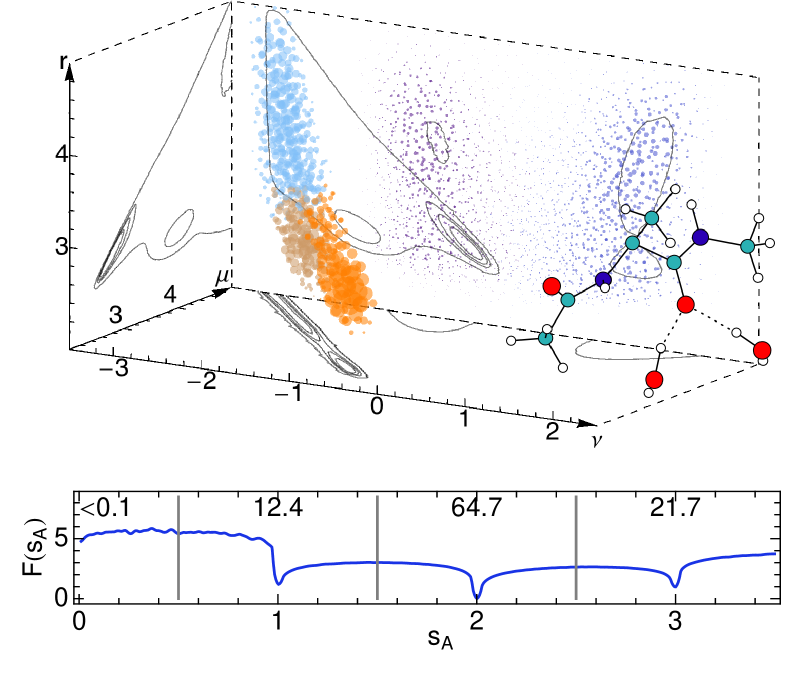
The first kind of HB we considered is O${}_{\text{w}}$–H$\cdots$O${}_{\text{C}}$. To accelerate the analysis we only included configurations with $\mu<5$Å. Figure 2 shows the distribution of the values of $(\nu,\mu,r)$, colored according to the partitioning of the density obtained by running PAMM on the data set. Several clusters are recognized, which means that besides HBs there are other recurring patterns that can be distinguished by this analysis. One of these clusters – represented with an orange hue – can be seen by direct inspection of configurations (or by comparison with other structural definitions) to correspond clearly to hydrogen-bonded configurations. As discussed in Section I we used the Gaussian-mixture model built based on the clustering to define the degree of confidence $s_{\text{DHA}}$ by which we classify a certain configuration of a D donor, H hydrogen and A acceptor as a hydrogen bond, and then introduce a count of the total HBs that involve a given acceptor oxygen $s_{\text{A}}=\sum_{\text{D},\text{H}}s_{\text{DHA}}$. The free energy built from the histogram of $s_{\text{A}}$ is represented in the lower panel of Figure 2. The free energy is strongly peaked at integer values of $s_{\text{A}}$, because the transition between 0 and 1 is very sharp when a hydrogen bond is formed or broken. This plot shows clearly that most of the time the carbonyl is involved in receiving two hydrogen bonds, but there is also a fairly large probability of accepting one or three bonds. It would be interesting to compare these results with first-principles simulations of solvated alanine dipeptide, to verify whether the possibility of forming over and under-coordinated configurations is a consequence of the simplified modelling of the interactions between water molecules and the carbonyl.

Figure 3: (Upper panel) Distribution of $(\nu,\mu,r)$ configurations for N–H$\cdots$O${}_{\text{w}}$ in a simulation of alanine dipeptide in water. Size and opacity of points correspond to the KDE of $P(\mathbf{y})$, and colors indicate the cluster each grid point has been assigned to. (Lower panel) Free energy (kcal/mol) computed from the distribution of number of donated hydrogen bonds $s_{\text{D}}$ for the amide nitrogen atom in solvated alanine dipeptide. See Fig. 2 for details. The average number of donated HBs is $\left<s_{\text{D}}\right>=1.3$ and the standard deviation is 0.5.

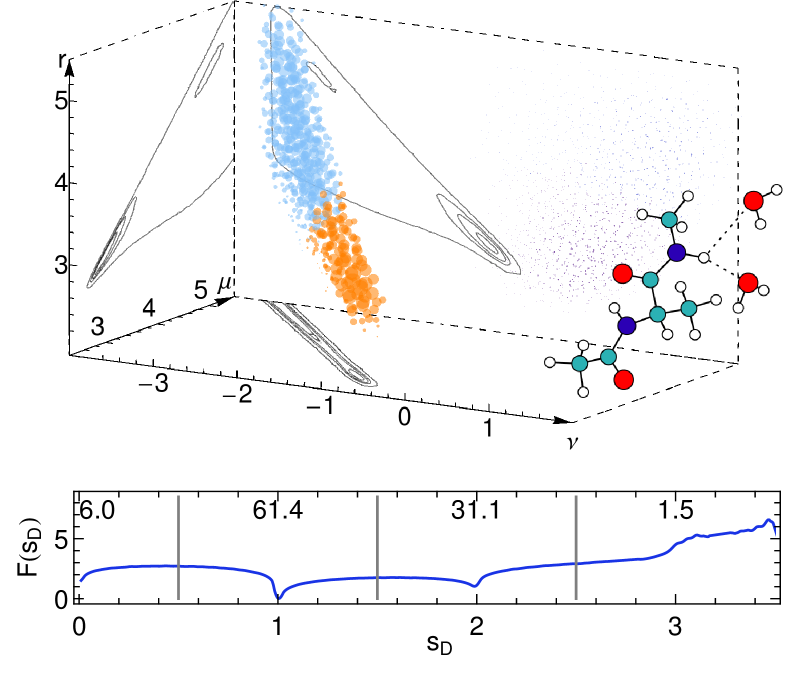
We then moved on to look into the hydrogen bond donated by the amide group N–H$\cdots$O${}_{\text{w}}$. Since the chemical identity of atoms is fixed in an empirical force field calculation, we specifically restricted the search to include only the amide H atom and oxygen atoms from the water molecules. We used a cut off of $\mu<5.5$Å to disregard configurations that are clearly irrelevant to the HB search. We report the distribution of configurations and the PAMM clustering in Figure 3. Perhaps unsurprisingly, the distribution of $(\nu,\mu,r)$ associated with this set of atoms differs considerably from that in Figure 2 – this is a somewhat weaker bond, which results in a less structured $P(\nu,\mu,r)$. Still, one can recognize a cluster that is clearly associated with HB configurations, that we can use to define a bond counting order parameter, that in turns can be used to compute the total number of hydrogen bonds donated by the N atom, $s_{\text{D}}=\sum_{\text{A},\text{H}}s_{\text{DHA}}$. While the most likely value of $s_{\text{D}}$ is one, there is a high probability of observing a N–H group donatinhg two HBs. Given the geometry of the amide group, this actually means that based on our unbiased, self-consistent definition, HBs donated by the amide group as described by the empirical forcefield we used have a large probability of being bifurcated, binding simultaneously to two different water molecules.

Figure 4: (Upper panel) Distribution of $(\nu,\mu,r)$ configurations for C_α–H$\cdots$O${}_{\text{w}}$ in a simulation of alanine dipeptide in water. Size and opacity of points correspond to the KDE of the $P(\mathbf{y})$, and colors indicate the cluster each grid point has been assigned to. (Lower panel) Free energy computed from the distribution of number of donated hydrogen bonds $s_{\text{D}}$ for the amide carbon atom in solvated alanine dipeptide. See Fig. 2 for details. The average number of donated HBs is $\left<s_{\text{D}}\right>=5.2$ and the standard deviation is 1.1.

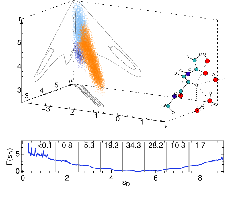
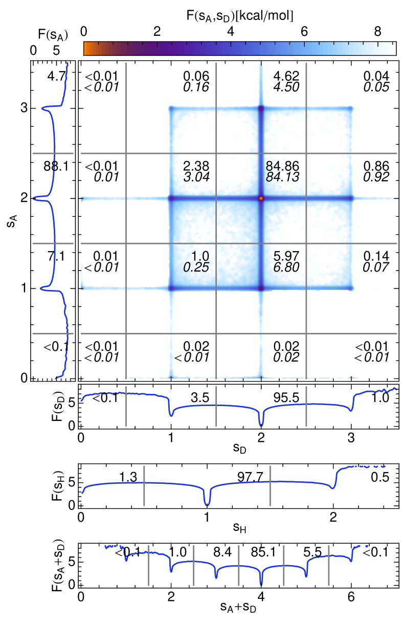
Finally, to verify how the PAMM algorithm behaves when applied to a selection of atoms that does not exemplify a typical hydrogen bond, we considered atom triplets that would correspond to a C_α–H group donating a HB to water. Figure 4 shows the partitioning of the probability density for this choice of atoms, which has some features that are reminiscent of those seen for conventional HBs, albeit with a much longer $d(\text{A--H})$. A more careful inspection of configurations that belong to the lobe of the probability density with the lowest $\mu$, however, shows that these can hardly be described as HBs: in many cases the hydrogen atoms of water molecules are oriented towards the C_α–H group, and the distribution of $s_{D}$ shows very little structure. This example demonstrates that the presence of a recurring structural motif with a signature in terms of the probability distribution in configuration space does not necessarily imply that the atoms that compose the motif are involved in some sort of chemical bonding. Here, the non-uniform structure of oxygen atoms in the vicinity of the C_α–H group is probably an indirect consequence of the hydrogen-bond interaction of water molecules with nearby carbonyl groups, and of the stiffness of the backbone of the dipeptide.

Water, classical and quantum

Figure 5: Distribution of $(\nu,\mu,r)$ configurations for O–H$\cdots$O^′ in a simulation of neat TIP4P water. Size and opacity of points correspond to the KDE of $P(\mathbf{y})$, and colors indicate the cluster each grid point has been assigned to. Clusters with $\nu>0$ have not been colored, but have been correctly identified by PAMM.

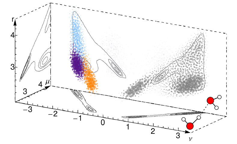
Simulations of alanine dipeptide contain different kinds of hydrogen bonds, and allowed us to demonstrate the adaptive nature of PAMM to derive a different, data-driven definition of the range of structural parameters that can be associated with a HB for each set of constituent atoms. In a simulation of neat water, instead, there is only one type of O–H$\cdots$O^′, the slight complication being that each oxygen atom can simultaneously act as a donor and an acceptor of hydrogen bonds.

TIP4P water.

We began by analyzing a simulation of a flexible TIP4P/2005fGonzález and Abascal (2011) model. A box containing 128 water molecules was first equilibrated for 2 ns at constant pressure (1 atm), constant temperature (298 K) NpT dynamics. A subsequent 500 ns NVT run was performed using a Langevin thermostat with relaxation time $\tau$=5 ps. The configurations were saved every 1 ps. In the spirit of a fully automated analysis of the trajectory, we did not exploit knowledge of the chemical identity of water molecules, which is fixed in a simulation with a non dissociable model. The distribution of $(\nu,\mu,r)$ shows clearly the dual role played by the O atoms (see Figure 5), which is apparent in the symmetry of the probability density across the $\nu=0$ plane. Both the cluster highlighted in orange and its mirror image correspond to legitimate HB configurations, but only the former corresponds to structures in which the first oxygen is acting as the donor and the second as the acceptor.

Figure 6: Hydrogen-bond counts statistics for a classical simulation of TIP4P water at room temperature. All the probability distributions have been smoothed with a triangular kernel of width 0.025, and are represented in terms of the associated free energies $F=-k_{B}T\ln P$, that are expressed in kcal/mol throughout. We also report integrated probabilities (in percent) to have a configuration in the vicinity of the different integer numbers of HBs. Below the values of the joint probabilities of $s_{\text{A}}$ and $s_{\text{D}}$ the product of marginal probabilities are indicated, in italics.

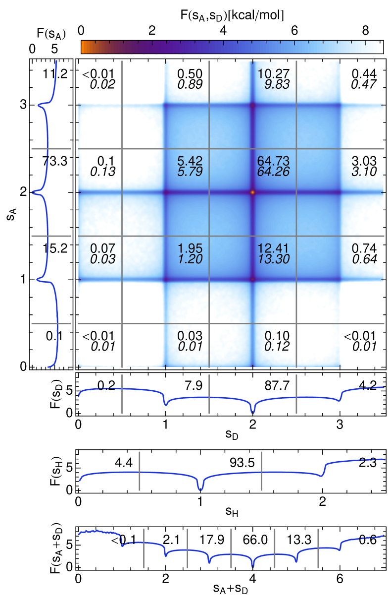
Once $s_{\text{DHA}}$ has been defined based on the analysis of the simulation data, it can be used to characterize in great detail how a given model of water describes hydrogen bonding. Figure 6 summarizes some of the information that can be obtained from this analysis. One can compute free energies for the number of hydrogen bonds donated ($s_{\text{D}}$) or accepted ($s_{\text{A}}$) by each oxygen atom, as well as for the total ($s_{\text{A}}+s_{\text{D}}$) and for the number of HBs that are formed by each hydrogen. A large fraction of TIP4P water molecules are tetracoordinated, with nearly 65% of oxygen atoms receiving and donating two HBs. There is a small but significant asymmetry between the distribution of $s_{\text{D}}$ and that of $s_{\text{A}}$, the former being more strongly peaked at $s_{\text{D}}=2$, while there is somewhat more flexibility in the count of accepted bonds. Given the rigid constraints on the covalent O–H bond, any oxygen in the simulation can donate two bonds at most, except for the case of bifurcated HBs where a single O–H moiety is involved with bonds to two different O^′ atoms. The distribution of $s_{\text{H}}$ shows that there is just about 2% probability of observing such bifurcated bonds. More detailed information on the topology of the HB network can be obtained by observing the joint probability distribution of $s_{\text{D}}$ and $s_{\text{A}}$. While the order of magnitude of the probability of each joint configuration is determined by the product of $s_{\text{D}}$ and $s_{\text{A}}$, there are significant deviations that are indicative of the correlations between defects in the network. For instance, the probability of having a “linear” water that donates and accepts a single HB is almost twice the value that would be expected based on the product of the marginal distributions. Note that this analysis focuses on the connectivity of the network rather than on the geometry of the environment of each water molecule. An interesting way to extend this analysis could consider the correlation between the HB counts and the degree of tetraedrality, with the electronic structure, or with quantities that can be directly related to experimental observables.

Figure 7: (Upper panel) Time correlation functions of the hydrogen-bond counts for a tagged oxygen in a simulation of TIP4P/2005f water. (Lower panel) Rate function for the hydrogen-bond formation/break-up, computed as the derivative of the correlation function $\left<s_{\text{DA}}(t)s_{\text{DA}}(0)\right>$

Dynamics of the HB network.

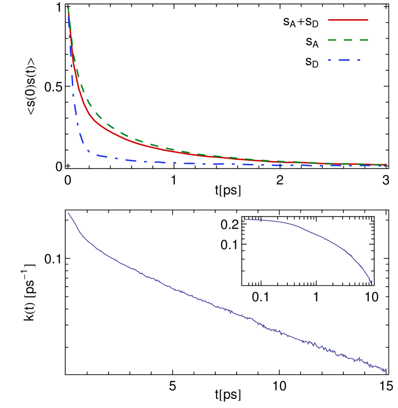
The asymmetry between $s_{\text{A}}$ and $s_{\text{D}}$ is also apparent when one considers the dynamical behavior of the two quantities. The upper panel of Figure 7 shows the correlation functions for the counts of acceptor and donor HBs for a tagged oxygen, as well as the total. They were computed analyzing several short NVE simulations started from independently equilibrated configurations. The correlation time of $s_{\text{D}}$ is very short, because configurations where a water molecule donates less or more than two HBs are very short-lived. Configurations that are distorted from the point of view of accepted HBs are less unstable, and therefore the correlation function of $s_{\text{A}}$ decays more slowly. The correlation function of the total is dominated by the slow decay of $s_{\text{A}}$, and is compatible with the results reported in Ref.Kumar et al. (2007) for traditional structural definitions of the hydrogen bond.

The hydrogen-bond count functions we have used this far do not consider the identity of individual bonds, so that a quick fluctuation that momentarily breaks a HB that is immediately re-formed is indistinguishable from a fluctuations that breaks a HB and leads immediately to the formation of a new HB with a different acceptor oxygen. A correlation function that is sensitive to the identity of the HB triplet, which is more easily interpreted in terms of physical observables,Luzar and Chandler (1996) can be readily computed by considering all the $(\text{D},\text{A})$ pairs, computing for each pair $s_{\text{AD}}=\sum_{\text{H}}s_{\text{DHA}}$. One can then compute the rate function as the time derivative of the autocorrelation of $s_{\text{AD}}$, computed for each pair separately:

$$k\left(t\right)=-\frac{1}{n_{\text{A}}n_{\text{D}}}\frac{\partial}{\partial t}\sum_{\text{A,D}}\left<s_{\text{AD}}(t)s_{\text{AD}}(0)\right>.$$ (12)

The decay takes place on a similar time scale than observed in Ref. Luzar and Chandler (1996), and exhibits similar features, including the presence of multiple time scales in the decay of the rate function.

Figure 8: Hydrogen-bond counts statistics for a classical simulation of BLYP water at room temperature. See the caption of Figure 6 for a detailed explanation of the plots.

Hydrogen-bonding defects in ice Ih

The consistency of the results obtained with PAMM descriptors of the hydrogen bond and those obtained with more conventional descriptors is reassuring. It is however useful to verify the behavior of indicators such as $s_{\text{A}}$ and $s_{\text{D}}$ in a more ordered environment such as the tetrahedral hydrogen-bond network of ice Ih, in which one should be able to identify clearly coordination defects.

Figure 9: a) Schematic representation of how a pair of Bjerrum defects are generated by flipping the orientation of a water molecule in a lattice that satisfies the ice rules. By flipping other molecules, the L and D defects can be separated. b) and c) Configurations of equilibrated L and D defects in ice Ih. Oxygen atoms with $s_{\text{A}}=1$ are colored in red, atoms with $s_{\text{A}}=3$ are colored in blue, while atoms with $s_{\text{A}}=s_{\text{D}}=2$ are in white, or hidden for clarity.

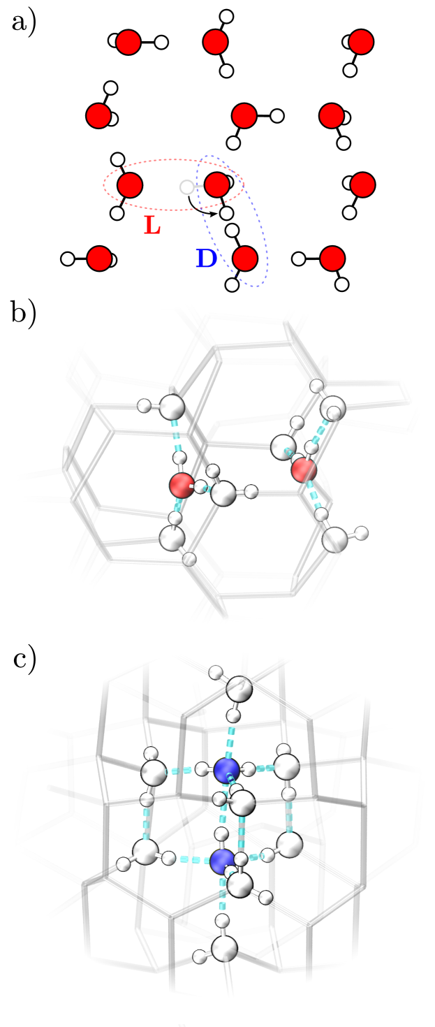
To this aim, we have performed a PAMM analysis of a simulation of ice Ih, using the same flexible TIP4P model discussed above, and a proton-disordered unit cell with 768 molecules Hayward and Reimers (1997). We have then created a pair of Bjerrum coordination defects Bjerrum (1952); de Koning et al. (2006), and separated them by the maximum distance allowed by the simulation cell, by repeatedly flipping water molecules in the lattice (Figure 9(a)). We have then equilibrated the simulation for a few tens of ps, collected some snapshots of the configurations and evaluated $s_{\text{A}}$ and $s_{\text{D}}$ for each oxygen. The vast majority of the O atoms have $s_{\text{A}}=s_{\text{D}}=2$, as one would expect in a perfect tetrahedral arrangement consistent with the ice rules. We could however identify clearly a pair of oxygen atoms with $s_{\text{A}}=1$ (a L defect), and a pair with $s_{\text{A}}=3$ (a relaxed D defect). Snapshots of these defective environments are represented in Figure 9.

Classical ab initio water.

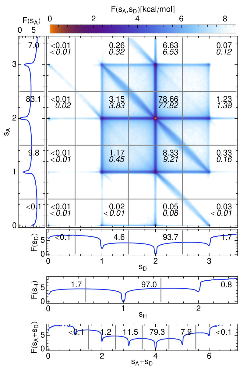
We then moved on to perform our analysis on a first-principles simulation of liquid water. The trajectory is the classical simulation from Ref. Ceriotti and Manolopoulos (2012), which was performed using the CP2K software package,VandeVondele et al. (2005); *goed+96prb with a BLYP exchange-correlation functionalBecke (1988); *lee+88prb and a DZVP basis set. The simulation box contained 64 water molecules at the experimental density, and 100 ps of NVT dynamics were performed, with the first 5 ps discarded for equilibration. A PAMM analysis of the simulation yielded very similar clusters to those obtained from TIP4P water. The analysis of HB counts, in Figure 8, shows that BLYP water has a very regular structure, with a higher count of tetracoordinated oxygen atoms, and a very low count of defective structures. This is consistent with the well-known observation that generalized-gradient approximation models of water are overstructured compared to experiment and to empirical water models. Note that correlations in the HB network are stronger in this case than for TIP4P water, with one-donor/one-acceptor oxygen atoms being four times more likely than one would expect given the separate probabilities of $s_{\text{A}}\approx 1$ and $s_{\text{D}}\approx 1$.

Figure 10: Hydrogen-bond counts statistics for a PIGLET simulation of BLYP water at room temperature. See the caption of Figure 6 for a detailed explanation of the plots.

Quantum ab initio water.

Finally, we considered a simulation that used the PIGLET technique to introduce nuclear quantum effectsCeriotti and Manolopoulos (2012) on top of a first-principles description of the electronic structure, analogous to the one used for the classical trajectory described above. To achieve convergence of quantum properties, 6 beads were used together with a custom-tailored generalized Langevin equation thermostat,Ceriotti (2010) as implemented in the i-PI Python interface.Ceriotti et al. (2014) The overall statistics of the HB network (Figure 10) are not dramatically changed by nuclear quantum effects, that only enhance marginally the probability of distorted configurations, with a decrease of ideal $(s_{\text{D}}\approx 2,s_{\text{A}}\approx 2)$ configurations and an increase of bifurcated hydrogen bonds. These are not however substantial changes, and are in part due to the fact that quantum fluctuations make the PAMM definition of $s_{\text{DHA}}$ less clear-cut than in the classical case.

Defining HBs with a method such as PAMM, that does not make any assumption on the covalent bonds present in the system, is particularly convenient in a context such as the present one. Extreme quantum fluctuations of protons along the hydrogen bond lead to transient formal autolysis events, where the hydrogen atom detaches from the donor atom and reaches out to be closer to the acceptor oxygen.Ceriotti et al. (2013) From a structural standpoint, PAMM does not recognize a distinct cluster corresponding to these distorted configurations, but rather a continuum of structures. Starting from a O₁–H$\cdots$O₂ bond where the hydrogen atom is covalently bound to O₁, one goes smoothly through distorted donated hydrogen bond to a configuration that is formally classified as a distorted bond accepted by O₁ and donated by O₂. These fluctuations conserve the total number of HBs between the two oxygen atoms, and only change their character from donated to accepted. These excursions are apparent in the joint probability distribution of $s_{\text{D}}$ and $s_{\text{A}}$, where they show up as regions with higher probability extending diagonally between two near-integer $(s_{\text{D}},s_{\text{A}})$ regions.

Liquid ammonia

As a final example, we considered liquid ammonia at 180K and ambient pressure. Configurations were kindly provided by Joshua More and David Manolopoulos.More and Manolopoulos (2014) Simulations were performed including nuclear quantum effects by path integral molecular dynamics, using 12 beads and PIGLETCeriotti and Manolopoulos (2012); Ceriotti (2010) as implemented in i-PI.Ceriotti et al. (2014) Quantum EspressoBaroni et al. was used as the force back-end, with a PBE exchange-correlation functionalPerdew et al. (1996) and ultra-soft pseudo-potentials.Vanderbilt (1990) The simulation box contained 32 molecules, and trajectories were performed for 10ps at constant, experimental density, with the first 2 ps discarded for equilibration.

Figure 11: Distribution of $(\nu,\mu,r)$ configurations for O–H$\cdots$O^′ in a simulation of liquid BLYP ammonia at 180K. Size and opacity of points correspond to the KDE of $P(\mathbf{y})$, and colors indicate the cluster each grid point has been assigned to. Clusters with $\nu>0$ have not been colored, but have been correctly identified by PAMM.

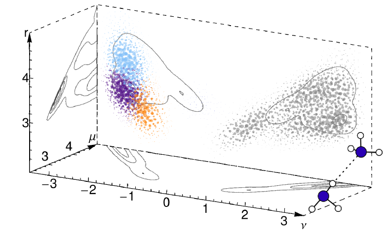
Ammonia is a less-structured liquid than water, with weaker hydrogen bonds, as it is already apparent from the probability density shown in Figure 11. Clusters are barely recognizable when using a two-dimensional $(\nu,r)$ representation, which was instead capable of characterizing the HB in all the other cases we considered. Clustering is much more evident using the three-dimensional $(\nu,\mu,r)$ description, and PAMM identifies clearly a range of values that can be ascribed to hydrogen-bonded configurations. We expect the observation that higher-dimensional descriptors offer increased discriminating power to be general, and provide a strategy to resolve weakly structured systems. However, as the dimensionality is increased it becomes more difficult to converge the probability distribution, so longer simulations are needed and PAMM becomes more sensitive to the parameters of the procedure. As it is the case for oxygen in H₂O, nitrogen atoms act both as donors and acceptors, leading to a symmetric structure for $P(\nu,\mu,r)$.

Figure 12: Hydrogen-bond counts statistics for a PIGLET simulation of BLYP liquid ammonia at 180K. See the caption of Figure 6 for a detailed explanation of the plots.

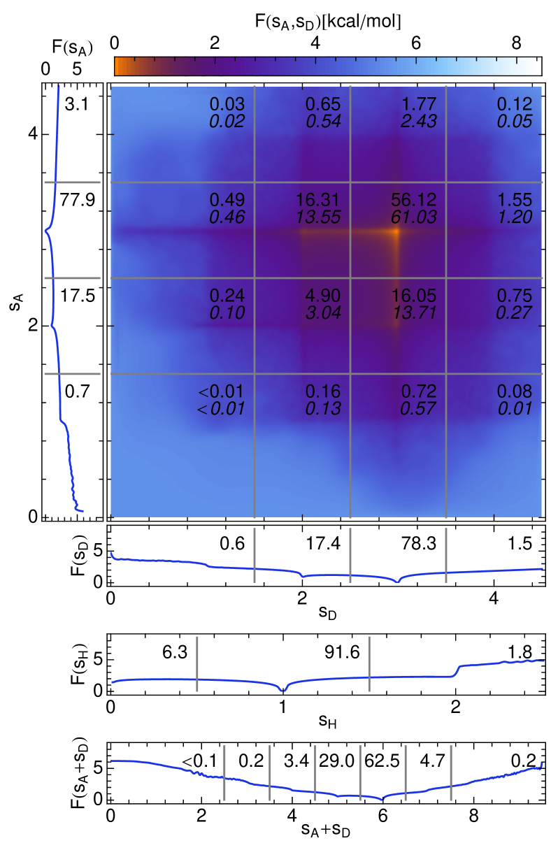
Figure 12 shows the analysis of the distribution of $s_{\text{D}}$, $s_{\text{A}}$ and $s_{\text{H}}$. Despite the low temperature, the weaker and less directional HBs result in a less clear-cut distribution of HB environments. A little more than 50% of the nitrogen atoms receive and donate 3 HBs – the ideal HB pattern that is observed in the solid phases of ammonia. Even though the simulation included nuclear quantum effects, there is no trace of the diagonal patterns that are a manifestation of extreme proton excursions along the hydrogen bond. Molecules maintain strictly their chemical integrity, and from a structural standpoint these weak HBs appear to have a purely electrostatic character.

Conclusions

The probabilistic analysis of molecular motifs algorithm we have introduced attempts to reproduce in an automatic, data-driven manner the process of recognizing recurring structural patterns that is behind our intuitive understanding of chemical bonding. It first performs a non-parametric partitioning of the probability distribution that characterizes the arrangement of a selected group of atoms in an atomistic simulation of a material or a compound. It then proceeds to model the clusters with a Gaussian mixture model that provides a natural, fuzzy definition of a chemical entity in terms of a smoothly varying posterior probability.

We demonstrate the effectiveness of this approach by applying PAMM to recognize an ubiquitous but hard to define entity as the hydrogen bond in a variety of different contexts. For each D–H$\cdots$A triplet of atoms, PAMM automatically identifies an appropriate range of structural parameters that provides an unbiased, agnostic definition of what constitutes a hydrogen bond for a given set of atoms and a particular atomistic model. In the case of an empirical forcefield model of solvated alanine dipeptide it identifies three (very different) ranges of configurations that qualify as a distinct, recurring patterns for the carbonyl oxygen accepting a HB from water, for the ammide nitrogen donating a HB to water, and for a hypothetical weak HB involving C_α atoms and water oxygens. In the latter case, the presence of a distinct feature in the probability distribution is probably an indirect effect of the structural correlations in the water HB network, of the HBs between water and the electro-negative atoms in alanine dipeptide and of the rigidity of the molecular backbone.

We then assessed the behavior of PAMM when performing a more detailed analysis of hydrogen bonding in water, comparing an empirical water model and a first-principles, density functional model of water with and without a description of the quantum nature of nuclei. We introduced a compact representation of the hydrogen-bonding properties of water molecules in terms of the total number of accepted and donated HBs, that arises naturally because PAMM identifies hydrogen-bonded configurations in terms of a smoothly varying HB count function. We demonstrated that these hydrogen bond counts can be used to study the dynamics of the hydrogen bond network, giving results that are fully compatible with well-established definitions of the hydrogen bond, and to identify coordination defects in the otherwise ideal HB network of ice Ih. This analysis also highlights the presence of characteristic features that are a signature of extreme excursions of protons along the hydrogen bond observed with a quantum description of nuclei. Finally, we discussed liquid ammonia as an example of a weakly hydrogen-bonded system, that shows a much less clear-cut partitioning of the probability distribution and a more varied ensemble of hydrogen-bonding molecular environments.

In all of these cases our algorithm provides an adaptive approach to define the hydrogen bond in a unique and unbiased way, that uses only structural information and that can be easily exploited to recognize correlation between the HB patterns involving a given molecule. Even though we have used hydrogen bonding as a representative benchmark, application of the PAMM algorithm is by no means limited to this example. It could be used to recognize complex structural patterns in a variety of materials and compounds, and be easily applied to bias molecular simulations to accelerate the interconversion between different (meta)stable atomic configurations.

Appendix A PAMM library and utilities

In the Supplementary Material we provide the source code of a simple Fortran90 library to perform PAMM analysis, and a tool to apply it to the case of the hydrogen bond si . Updated versions of the package will be made available on http://epfl-cosmo.github.io. The workflow for using this software follows closely the procedure introduced in Section I. Starting from a preliminary simulation, one should first extract representative descriptors for the atom groups that are being studied. Here, one can use the hbpamm utility to process a set of atomic configurations in xyz format, to generate a list of $(\nu,\mu,r)$ triplets. Then, the pamm tool can use this data to generate a probabilistic model that describes the range of structural parameters associated with the hydrogen bond. This piece of code is completely general, and can be used to process any sort of structural data. Finally, one should use once more hbpamm (or an analogous utility adapted to a different kind of structure) to post-process the trajectory, extracting $s_{\text{A}}$, $s_{\text{D}}$, $s_{\text{H}}$ for the different atoms considered.

References

- Pauling (1960) L. Pauling, The nature of the chemical bond and the structure of molecules and crystals: an introduction to modern structural chemistry, Vol. 18 (Cornell University Press, 1960).
- Car and Parrinello (1985) R. Car and M. Parrinello, Phys. Rev. Lett. 55, 2471 (1985).
- Schaefer III (2012) H. F. Schaefer III, Quantum chemistry: the development of ab initio methods in molecular electronic structure theory (Courier Dover Publications, 2012).
- MacKerell et al. (1998) A. D. MacKerell, D. Bashford, M. Bellott, R. L. Dunbrack, J. D. Evanseck, M. J. Field, S. Fischer, J. Gao, H. Guo, S. a. Ha, and others, The Journal of Physical Chemistry B 102, 3586 (1998).
- Behler and Parrinello (2007) J. Behler and M. Parrinello, Phys. Rev. Lett. 98, 146401 (2007).
- Bartók et al. (2010) A. P. Bartók, M. C. Payne, R. Kondor, and G. Csányi, Phys. Rev. Lett. 104, 136403 (2010).
- Pauling (1928) L. Pauling, Proceedings of the National Academy of Sciences of the United States of America 14, 359 (1928).
- Pauling et al. (1951) L. Pauling, R. B. Corey, and H. R. Branson, Proceedings of the National Academy of Sciences 37, 205 (1951).
- Guo and Karplus (1994) H. Guo and M. Karplus, The Journal of Physical Chemistry 98, 7104 (1994).
- Jeffrey (1997) G. A. Jeffrey, An introduction to hydrogen bonding, Vol. 12 (Oxford university press New York, 1997).
- Desiraju and Steiner (2001) G. R. Desiraju and T. Steiner, Weak hydrogen Bond (Oxford University Press New York, 2001).
- Lin et al. (2011) L. Lin, J. a. Morrone, and R. Car, J. Stat. Phys. 145, 365 (2011).
- McKenzie et al. (2014) R. H. McKenzie, C. Bekker, B. Athokpam, and S. G. Ramesh, J. Chem. Phys. 140, 174508 (2014).
- Weinhold and Klein (2012) F. Weinhold and R. A. Klein, Molecular Physics 110, 565 (2012).
- Wendler et al. (2010) K. Wendler, J. Thar, S. Zahn, and B. Kirchner, J. Phys. Chem. A 114, 9529 (2010).
- Azar and Head-Gordon (2012) R. J. Azar and M. Head-Gordon, The Journal of Chemical Physics 136, 024103 (2012).
- Weinhold and Klein (2014) F. Weinhold and R. A. Klein, Chemistry Education Research and Practice (2014), 10.1039/c4rp00030g.
- Kühne and Khaliullin (2014) T. D. Kühne and R. Z. Khaliullin, J. Am. Chem. Soc. 136, 3395 (2014).
- Vedaldi and Soatto (2008) A. Vedaldi and S. Soatto, in Computer Vision-ECCV 2008 (Springer, 2008) pp. 705–718.
- (20) See Supplementary Material Document No. xxxxxx for a detailed discussion of the stability of the algorithm, a library of tools to apply PAMM, and the input files to reproduce the simulations described in the text.
- Gallet and Pietrucci (2013) G. Gallet and F. Pietrucci, J. Chem. Phys. 139, 074101 (2013).
- Note (1) In practice, one can almost invariably introduce a cutoff to avoid considering tuples that involve atoms that are very far away from each other, and hence clearly unrelated.
- Silverman (1986) B. W. Silverman, Density estimation for statistics and data analysis, Vol. 26 (CRC press, 1986).
- Eldar et al. (1997) Y. Eldar, M. Lindenbaum, M. Porat, and Y. Y. Zeevi, IEEE Trans. Image Process. 6, 1305 (1997).
- Note (2) As a trivial example of such weights, consider the normalization that is used to define the radial distribution function between a pair of atoms based on the histogram of the pairwise distances .
- Comaniciu and Meer (2002) D. Comaniciu and P. Meer, IEEE Trans. Pattern Anal. Mach. Intell. 24, 603 (2002).
- Note (3) Quick shift is not particularly sensitive to the choice of We found it convenient to set , where the are the kernel widths associated with the grid points. The SM si .
- Note (4) Quick shift is a medoid method, and as such the modes it finds are bound to be grid points. This means that the resolution of the grid impacts the definition of the cluster centers. In practice, this is easily solved by quickly optimizing the positions of the points using mean shift.
- Press (2007) W. H. Press, Numerical Recipes: The art of scientific computing (Cambridge University Press, 2007).
- Reynolds (2009) D. Reynolds, Encyclopedia of Biometrics , 659 (2009).
- Maragakis et al. (2009) P. Maragakis, A. van der Vaart, and M. Karplus, J. Phys. Chem. B 113, 4664 (2009).
- Tribello et al. (2010) G. A. Tribello, M. Ceriotti, and M. Parrinello, Proc. Natl. Acad. Sci. USA U. S. A. 107, 17509 (2010).
- Pisani et al. (2014) P. Pisani, P. Piro, S. Decherchi, G. Bottegoni, D. Sona, V. Murino, W. Rocchia, and A. Cavalli, J. Chem. Theory Comput. 10, 2557 (2014).
- Laio and Parrinello (2002) A. Laio and M. Parrinello, Proc. Natl. Acad. Sci. USA 99, 12562 (2002).
- Pietrucci and Andreoni (2011) F. Pietrucci and W. Andreoni, Phys. Rev. Lett. 107, 085504 (2011).
- Sadeghi and Ghasemi (2013) A. Sadeghi and S. Ghasemi, J. Chem. Phys. 139, 184118 (2013).
- Ferguson et al. (2010) A. L. Ferguson, A. Z. Panagiotopoulos, P. G. Debenedetti, and I. G. Kevrekidis, Proc. Natl. Acad. Sci. USA U. S. A. 107, 13597 (2010).
- Tribello et al. (2012) G. A. Tribello, M. Ceriotti, and M. Parrinello, Proc. Natl. Acad. Sci. USA U. S. A. 109, 5196 (2012).
- Rohrdanz et al. (2013) M. a. Rohrdanz, W. Zheng, and C. Clementi, Annu. Rev. Phys. Chem. 64, 295 (2013).
- Desiraju (2011) G. R. Desiraju, Angew. Chem. Int. Ed. Engl. 50, 52 (2011).
- Arunan et al. (2011) E. Arunan, G. R. Desiraju, R. A. Klein, J. Sadlej, S. Scheiner, I. Alkorta, D. C. Clary, R. H. Crabtree, J. J. Dannenberg, and P. Hobza, Pure and applied chemistry 83, 1637 (2011).
- Derewenda et al. (1995) Z. S. Derewenda, L. Lee, and U. Derewenda, Journal of molecular biology 252, 248 (1995).
- Reed et al. (1988) A. E. Reed, L. A. Curtiss, and F. Weinhold, Chemical Reviews 88, 899 (1988).
- Pendás et al. (2006) A. M. Pendás, M. Blanco, and E. Francisco, The Journal of chemical physics 125, 184112 (2006).
- Taylor and Kennard (1984) R. Taylor and O. Kennard, Accounts of chemical research 17, 320 (1984).
- Matsumoto (2007) M. Matsumoto, The Journal of chemical physics 126, 054503 (2007).
- Kumar et al. (2007) R. Kumar, J. R. Schmidt, and J. L. Skinner, J. Chem. Phys. 126, 204107 (2007).
- Jorgensen et al. (1983) W. L. Jorgensen, J. Chandrasekhar, J. D. Madura, R. W. Impey, and M. L. Klein, The Journal of chemical physics 79, 926 (1983).
- Plimpton (1995) S. Plimpton, J. Comput. Phys. 117, 1 (1995).
- Schneider and Stoll (1978) T. Schneider and E. Stoll, Phys. Rev. B 17, 1302 (1978).
- González and Abascal (2011) M. A. González and J. L. F. Abascal, The Journal of Chemical Physics 135, 224516 (2011).
- Luzar and Chandler (1996) A. Luzar and D. Chandler, Nature 379, 55 (1996).
- Hayward and Reimers (1997) J. A. Hayward and J. R. Reimers, J. Chem. Phys. 106, 1518 (1997).
- Bjerrum (1952) N. Bjerrum, Science 115, 385 (1952).
- de Koning et al. (2006) M. de Koning, A. Antonelli, A. J. da Silva, and A. Fazzio, Physical review letters 96, 075501 (2006).
- Ceriotti and Manolopoulos (2012) M. Ceriotti and D. E. Manolopoulos, Phys. Rev. Lett. 109, 100604 (2012).
- VandeVondele et al. (2005) J. VandeVondele, M. Krack, F. Mohamed, M. Parrinello, T. Chassaing, and J. Hutter, Comput. Phys. Commun. 167, 103 (2005).
- Goedecker et al. (1996) S. Goedecker, M. Teter, and J. Hutter, Phys. Rev. B 54, 1703 (1996).
- Becke (1988) A. D. Becke, Phys. Rev. A 38, 3098 (1988).
- Lee et al. (1988) C. Lee, W. Yang, and R. G. Parr, Phys. Rev. B 37, 785 (1988).
- Ceriotti (2010) M. Ceriotti, “GLE4MD,” http://epfl-cosmo.github.io/gle4md (2010).
- Ceriotti et al. (2014) M. Ceriotti, J. More, and D. E. Manolopoulos, Comput. Phys. Commun. 185, 1019 (2014).
- Ceriotti et al. (2013) M. Ceriotti, J. Cuny, M. Parrinello, and D. E. Manolopoulos, Proc. Natl. Acad. Sci. USA U. S. A. 110, 15591 (2013).
- More and Manolopoulos (2014) J. More and D. Manolopoulos, private communication (2014).
- (65) S. Baroni, A. Dal Corso, S. de Gironcoli, P. Giannozzi, C. Cavazzoni, G. Ballabio, S. Scandolo, G. Chiarotti, P. Focher, A. Pasquarello, K. Laasonen, A. Trave, R. Car, N. Marzari, and A. Kokalj, “PWSCF,” .
- Perdew et al. (1996) J. P. Perdew, K. Burke, and M. Ernzerhof, Phys. Rev. Lett. Phys. Rev. Lett. (USA), 77, 3865 (1996).
- Vanderbilt (1990) D. Vanderbilt, Phys. Rev. B 41, 7892 (1990).