An Efficient Non-Intrusive Uncertainty Propagation Method for Stochastic Multi-Physics Models
Abstract
Multi-physics models governed by coupled partial differential equation (PDE) systems, are naturally suited for partitioned, or modular numerical solution strategies. Although widely used in tackling deterministic coupled models, several challenges arise in extending the benefits of modularization to uncertainty propagation. On one hand, Monte-Carlo (MC) based methods are prohibitively expensive as the cost of each deterministic PDE solve is usually quite large, while on the other hand, even if each module contains a moderate number of uncertain parameters, implementing spectral methods on the combined high-dimensional parameter space can be prohibitively expensive. In this work, we present a reduced non-intrusive spectral projection (NISP) based uncertainty propagation method which separates and modularizes the uncertainty propagation task in each subproblem using block Gauss-Seidel (BGS) techniques. The overall computational costs in the proposed method are also mitigated by constructing reduced approximations of the input data entering each module. These reduced approximations and the corresponding quadrature rules are constructed via simple linear algebra transformations. We describe these components of the proposed algorithm assuming a generalized polynomial chaos (gPC) model of the stochastic solutions. We demonstrate our proposed method and its computational gains over the standard NISP method using numerical examples.
keywords:
Multi-physics Models, Stochastic Modeling, Polynomial Chaos, Non-Intrusive Spectral Projection.AMS:
60H15, 60H30, 60H35, 65C30, 65C501 Introduction
With the aim of validating predictions from computer simulations against real-world experiments, it becomes necessary to include uncertainties (descrbied as random quantities) within the associated physical model. Uncertainties of this kind, known as aleatoric uncertainties, mainly arise because mathematical models are often idealized approximations of their target scenarios (in terms of geometry, material properties and boundary constraints ), and due to limited knowledge in defining parameters of the physical systems being investigated. Uncertainty Quantification (UQ) tools, have therefore, become key requirements for estimating the credibility and confidence of predictions from computer simulations. In particular, addressing the computationally demanding task of uncertainty propagation, has gained tremendous prominence amongst simulation engineers, supported by the rapid growth in computing power and advances in numerical analysis.
To this end, Monte-Carlo (MC) based methods [1, 2], wherein the corresponding ouput samples for a set of random input samples can be collected via repeated simulation runs, provide the most straightforward approach. However, when dealing with costly PDE solvers, computing an ensemble of output realizations large enough to evaluate accurate statistics can be prohibitively expensive. Alternatively, cheaper surrogate models, can be trained on a much smaller ensemble of solution samples, using various sparse regression techniques [3, 4], and subsequently sampled exhaustively to approximate solution distributions and/or statistics. However, in the context of multi-physics problems, or coupled PDE systems in general, these methods ignore the rich and potentially exploitable structures within the model.
Several coupled PDE systems, for example, fluid-structure [5] and reactive-transport models [6], are natural targets for employing modular (partitioned) solution methods wherein, solvers can be rapidly developed by reusing legacy solvers for each constituent subproblem. The disadvantage however, is that the convergence rate of modular methods, can be much slower when compared to monolithic methods, for example, the quadratically convergent Newton’s method [7]. Therefore, in the context of coupled PDE solvers, modularization typically results in a trade-off between the developmental and computational costs, of which the former usually dominates. However, in extending the standard practices of modularization towards uncertainty propagation, several challenges yet remain.
In this work, we propose an efficient non-intrusive method for generalized polynomial chaos (gPC) [8] based uncertainty propagation in coupled PDE solvers, which mitigates the curse of dimensionality associated with spectral uncertainty propagation methods. This is achieved by constructing reduced dimensional (and order) approximations of the input data are before they enter their respective solver modules. Correspondingly, reduced approximations of the respective output data are obtained using optimal quadrature rules, which consequently reduce the required number of repeated module runs significantly. Simple linear algebraic tools are used in constructing the reduced approximations and quadrature rules. Moreover, the approximation errors can be controlled separately in each module. While several recent works have demonstrated the possibility of exploiting relatively trivial coupling structures, for example, unidirectional coupling [9], and linear coupling [10, 11, 12], to reduce the costs of uncertainty propagation, we consider a more general setup with bidirectional and nonlinear coupling structures in this work.
Our proposed method is a generalization of the approach recently proposed by Constantine et. al [13], which applies well to network (weakly) coupled multi-physics systems. Moreover, several components of our proposed algorithm have also been motivated by the recent works of Arnst et. al. [14, 15], wherein reduced chaos expansions [16] are used in approximating the input data. However, in their approach, the dimension reduction procedure can only be implemented unidirectionally, and therefore, the computational gains achieved would be limited to those respective modules only. We address this limitation in our proposed method and facilitate the reduction strategy to be implemented across all the modules. Furthermore, the respective tolerances, which control the error in the reduced approximations, can be prescribed individually for each module.
The remainder of this article is organized as follows. In §2, we provide an overview of the preliminary definitions and concepts, along with a description of the standard non-intrusive spectral projection (NISP) method for solving stochastic algebraic systems. In §3, we describe the proposed reduced NISP method and its constituent dimension and order reduction steps. Moreover, we prove the existence of asymptotic upper bounds on the approximation errors incurred by our proposed method. In §4, we report and compare the performance and accuracy of the standard and reduced NISP method implementations on two numerical examples.
2 Preliminary definitions and concepts
Without loss of generality, we focus our analysis on a two component, steady-state coupled PDE system. First, we consider the deterministic case.
2.1 Deterministic model
A spatial discretization of the system yields the coupled algebraic system:
| (1) |
where , denote the discrete component residuals and , denote the respective finite-dimensional discretizations of the solution fields intrinsic in each component PDE system.
2.2 Deterministic numerical solvers
There are various approaches to solve Eq. 2.1 numerically. Monolithic solution methods, for example, Newton’s method, would require repeatedly solving the fully-coupled linear system
| (2) |
to compute the solution updates. In general, developing a solver for this linear system from scratch is quite challenging. Moreover, if legacy solvers for each subproblem: and , are available, extensive modifications to their respective source codes would be required to construct the Jacobian in Eq. 2.2. Furthermore, the quadratic convergence rate of Newton’s method is not always guaranteed in practice. These limitations can be primarily attributed to the bidirectional nature of the coupled PDE system and the influence of the off-diagonal blocks and in the linear system. Variants of Newton’s method such as Broyden’s method [17], Gauss-Newton [18] and Levenberg-Marquardt [19], would also be affected by these limitations, if implemented in this monolithic fashion.
Therefore, modular approaches, for example, block-Gauss-Seidel (BGS) [20], can overcome some of these limitations of monolithic methods, and are often preferred in practice. The primary advantage of modularization is that legacy solvers with disparate discretization and solution techniques can be easily coupled with minimal modifications to their source codes. In general, the BGS method is an iterative method which can be represented as
| (3) |
where and denote the computational modules. Individually, these modules can also be used to solve , given and , given respectively.
2.3 Stochastic model
We now consider the case where and are each dependent on a set of random input parameters, denoted as and respectively. Let , denote the respective probability density functions of and . Moreover, we assume that the input parameters as well as their individual elements are statistically independent. Let denote the combined parameter space with dimension and ,
| (4) |
denote the corresponding joint probability density function.
Retaining the structure and dimensions of the deterministic algebraic system in Eq. 2.1, the stochastic nonlinear system of equations are now formulated as follows.
| (5) |
We assume that , the iterations
| (6) |
are to converge to a solution of Eq. 2.5. A general formulation of a two-component coupled stochastic algebraic system
| (7) |
where and denote the coupling or interface functions can be solved with a modified BGS method, wherein , the iterations
| (8) |
converge to a solution of Eq. 2.7.
2.4 Generalized polynomial chaos
, let denote the symmetric-positive-definite Gramian matrix [21] corresponding to . Moreover, let
| (9) |
denote the space of -weighted, -square integrable functions that map from to . If , then it can be represented exactly as an infinite polynomial series as follows. ,
| (10) |
where denotes the set of -orthonormal polynomials, and a basis for all -weighted, square-integrable scalar functions in . The statistical independence of the coordinate directions in implies that each basis polynomial is a product of univariate orthonormal polynomials [22], which in turn can be precomputed using the Golub-Welsch algorithm [23]. Moreover, the indexing in the polynomial series is assumed to follow a total degree ordering, such that
| (11) |
where , denotes the total degree of .
Consequently, a gPC [8] approximation ,
| (12) |
with order and gPC coefficients can be formulated as a finite truncation of Eq. 2.10, where denotes the gPC coefficient matrix and denotes the basis vector. If the truncation is isotropic and based on the total degree, then and are related as follows.
| (13) |
The orthonormality of the elements in yields the spectral projection formula
| (14) |
Moreover, the Cameron-Martin theorem [24] states that if is infinitely regular in , then as , the gPC approximation converges exponentially to , in the mean-square sense. To state this formally, , such that ,
| (15) |
for some . Furthermore, a corollary to the theorem states that if the regularity of is , then the asymptotic rate of convergence is polynomial and the upper bound in the mean-square error would be .
When compared to repeated executions of a costly numerical PDE solver, the gPC approximation can be used as a significantly cheaper surrogate model for computing statistical quantities of interest such as the moments and probability density functions of via exhaustive sampling. In particular, approximations of the first two moments can be computed directly from the gPC coefficients as follows.
| (16) |
Moreover, the probability density function of any related quantity of interest can be computed with the kernel density estimation (KDE) method [25], by generating a large number of samples of the cheaper polynomial surrogates. Therefore, prior to any uncertainty analysis, the gPC coefficient matrices of the solutions must be computed via uncertainty propagation. In this work, we focus on the non-intrusive projection method [26], which enables the reuse of the solver components and .
2.5 Non-intrusive spectral projection
Non-intrusive spectral projection (NISP), is a method to approximate the gPC coefficients by approximating the integration in the spectral projection formula in Eq. 2.14 using a quadrature rule in in , denoted as . Therefore, ,
| (17) |
If denotes the level of the quadrature rule, then all polynomials with a total degree can be numerically integrated using the quadrature rule, up to machine precision. The relation between and depends on the type of quadrature rule implemented. For instance, employing a full grid tensorization of univariate Gauss-quadrature rules yields the relation , while for the same level , sparse grids [27] exhibit a much slower, albeit exponential growth in . This exponential growth phenomenon is commonly known as the curse of dimension.
2.5.1 Algorithm and computational cost
Algorithm 1 describes the standard NISP based uncertainty propagation method.
, the precomputed matrix
| (18) |
denotes the gPC coefficient matrix of the random input .
We assume that the computational costs are dominated by the repeated execution of module operators and . Let denote the average cost of executing of and denote the average cost of executing of . Therefore, the computational cost of the standard NISP method
| (19) |
would grow exponentially with respect to the dimension and order . To mitigate these costs, we propose a reduced NISP based uncertainty propagation method, which will be described in the next section.
3 Reduced NISP based uncertainty propagation
Our proposed method is a modification of Algorithm 1 with the addition of two intermediate computational steps at each iteration: (1) a dimension reduction routine, and (2) an order reduction routine.
3.1 Dimension reduction
At each iteration , let and denote the input data that enter and respectively. Moreover, let
| (20) |
denote the Gramian matrices and
| (21) |
as the gPC coefficient matrices corresponding to and respectively. Subsequently, , we construct
| (22) |
by deleting the first column of , and left multiplying the resultant matrix with . The singular value decomposition (SVD) of
| (23) |
is computed, wherein the constituent matrices have the following structure and dimensions.
| (25) | ||||
| (29) | ||||
| (33) |
We then construct
| (34) |
and
| (35) |
denotes the -th uncorrelated random variable with zero mean and unit variance that enters the component . The expansion in Eq. 3.10 is the finite-dimensional variant of the Karhunen-Loeve (KL) expansion [28], which is widely used as an approximation of spatiotemporal random fields.
3.1.1 Reduced dimensional KL expansion
and iteration , the expansion (3.10) can be truncated by retaining terms to define an approximation ,
| (38) |
Let denote the reduced dimensional random vector with a probability density function . Moreover, we let denote the affine map which defines the composition , such that ,
| (39) |
where
| (40) |
and
| (41) |
Furthermore, we extract the following subvector and submatrix blocks from and respectively.
| (42) |
| (43) |
where , , , and , , , , , define the affine maps corresponding to respectively.
3.1.2 Selecting the reduced dimensions
, we prescribe a tolerance such that, at each iteration , is selected as the minimum which satisfies
| (44) |
If , then a reduced dimensional approximation of the input data in module exists, with an approximation error . Theorem 1 proves this error bound.
Theorem 1:
and iteration , the approximation satisfies the inequality
| (45) |
Proof:
The square of the left hand side expression in Eq. 3.19 can be written as follows.
| (52) | |||
| (55) | |||
| (61) | |||
| (68) | |||
| (75) |
In the context of the modified coupled model with interface functions in Eq. 2.7, the dimension reduction procedure would be exactly the same as described here with the exception that the input data are formulated as as and respectively.
3.2 Order reduction
As described in §3.1, and iteration , an approximation of the input data that enters the solver component can be constructed in the reduced dimensional stochastic space .
For any square-integrable, vector-valued function , a reduced gPC approximation of order can be formulated as follows. ,
| (77) |
where denotes the set of -orthonormal polynomials, denotes the reduced order gPC coefficient matrix and denotes the reduced order basis vector. If the formulation of the gPC approximation is based on an isotropic, total degree truncation of the infinite polynomial series, then and are related as follows.
| (78) |
Moreover, we assume that , which implies that .
Since the coordinate directions in are not necessarily statistically independent, we cannot simply compute the elements of as products of univariate polynomials. Instead, we propose a SVD based numerical construction method.
3.2.1 Reduced order basis construction
, iteration and degree index , let ,
| (79) |
denote the monomial function with . The number of such monomial functions with a total degree is equal to . Let denote the corresponding set of indices and denote the monomial vector.
The monomial vector defines the corresponding Hankel matrix
| (80) |
which in turn can be approximated using the global quadrature rule as follows.
| (81) |
In general, the basis vector could be computed as follows. ,
| (82) |
where is the lower triangular matrix which defines the Cholesky factorization . However, the possibility of negative weights in the quadrature rule can lead to zero or negative eigenvalues in the approximation . Therefore, we instead compute the rank-reduced SVD of
| (83) |
where denote the usual decomposition matrices and denotes a diagonal matrix with as its diagonal elements. Since is symmetric, such a decomposition will always exist [29].
Subsequently, the basis vector is computed as follows. ,
| (84) |
Here, satisfies the discrete orthogonality condition
| (85) |
and therefore, defines the reduced spectral projection formula
| (86) |
Eq. 3.31 implies that is a quadrature rule of level in . However, depends exponentially on the global dimension and gPC order , implying that the quadrature rule is not computationally optimal with respect to the reduced dimension and gPC order . Therefore, we propose a QR factorization based method to construct the computationally optimal quadrature rule in , the size of which depends exponentially on and .
3.2.2 Optimal quadrature rule construction
and iteration , an optimally sparse quadrature rule of level in , denoted as , would contain the minimum possible number of non-zero weights and be able to numerically integrate all polynomials with total degree , up to machine precision. This requirement is dictated by the reduced spectral projection formula in Eq. 3.31.
Therefore, if and denote the dense and optimally sparse weight vectors respectively, then solves the minimization problem:
| (87) |
where
| (88) |
denotes the corresponding Vandermonde matrix with rows. In general, may not be full rank and therefore, we can setup a numerically stable and equivalent minimization problem as follows.
| (89) |
where is the rank of and defines the pivoted-QR factorization of
| (90) |
Instead of solving the NP-hard minimization problem, we employ a direct approach to construct a ’weakly’ optimal quadrature rule, which has at most non-zero weights. Therefore, we compute the pivoted-QR factorization of :
| (91) |
construct the upper triangular square matrix using first columns of , and compute the sparse weight vector as follows.
| (92) |
If denotes the index set corresponding to the non-zero elements in , then the reduced spectral projection formula in Eq. 3.31 can be efficiently computed as follows.
| (93) |
Using Eq. 3.38, the global gPC coefficient matrix of can be subsequently approximated as follows.
| (94) |
In general, the level and characteristics of the global quadrature rule used in approximating the global spectral projection formula (Eq. 3.39) can differ from the level and characteristics of the global quadrature rule used in constructing the optimally sparse quadrature rule. Moreover, a strictly positive weight vector with non-zeros can be computed using the Nelder-Mead method [30], in which case, the upper bound of on the sparsity of the optimal weight vector would coincide with the upper bound proved by Tchakaloff theorem [31]. Furthermore, the sparsity can also be explicitly controlled by prescribing a threshold on the diagonal elements of .
3.2.3 Selecting the reduced representation
, we prescribe a tolerance such that, at each iteration , the reduced order is selected as the smallest , which satisfies
| (95) |
where denotes the -weighted Frobenius norm, such that .
We propose the following heuristic to select . is initialized to at , and subsequently incremented by at any , if . Therefore, by choosing an appropriate value for the tolerance , we can guarantee that and therefore, a reduction of the gPC approximation order. Moreover, the requirement of computing implies that the level of the constructed optimal quadrature rule must be .
Theorem 2:
and iteration , let denote an infinitely regular vector valued function in and its reduced gPC approximation of order respectively. Given a positive-definite Gramian , if and denote the respective global gPC approximations of the composite functions and , then , such that ,
| (96) |
for some .
Proof:
Since is infinitely regular in , is infinitely regular in . Therefore, from the Cameron-Martin theorem, , such that for any positive-definite , the approximation error between and has the following upper bound.
3.3 Algorithm and computational cost
The proposed reduced NISP based uncertainty propagation method is described in Algorithm 2. Let denote the size of the optimal quadrature rule corresponding to the reduced dimension and reduced order , and let denote the size of the optimal quadrature rule corresponding to the reduced dimension and reduced order . Therefore, retaining the assumption that the computational costs are dominated by the repeated execution of module operators and , the computational cost of the reduced NISP method
| (98) |
would grow exponentially with respect to the reduced dimensions and orders . Therefore, the proposed reduced NISP method indeed mitigates the curse of dimensionality associated with the standard NISP method.
3.4 Error analysis
, let ,
| (99) |
denote the mean-square erro between the component solution and its corresponding reduced gPC approximation .
Subsequently, can be decompoed as a sum of individual error terms as follows.
| (100) |
where denotes the convergence error, denotes the gPC truncation error, denotes the reduced dimension approximation error and denotes the reduced order approximation error. Using the triangle inequality property of norms, an asymptotic upper bound for each constituent error term can be formulated as follows. ,
| (101) |
In the standard NISP method, the asymptotic upper bound on the approximation error would simply be the sum of the first two terms on the right hand side of Eq. 3.46, implying that would converge to as . However, in the reduced NISP method, would converge to a non-zero quantity, and have an asymptotic upper bound of .
This analysis suggests that the approximation error in can be explicitly controlled by choosing the tolerances and appropriately.
3.5 Selecting the tolerance values
In practice, since the exact bounds on the approximation error are not known apriori, the tolerance values are selected based on the results computed in a preliminary study, wherein a lower fidelity multi-physics model is used and the various tolerance values can be tested. In our case, lower fidelity translates to a coarser spatial discretization of the original steady state coupled PDE system to formulate the coupled algebraic system. An illustration of this is provided in the numerical experiments in §4
4 Numerical examples
We will now demonstrate and compare the performance of the standard and reduced NISP methods using two numerical examples.
4.1 Poisson problem
The Poisson problem is a widely used numerical example for benchmarking uncertainty propagation methods [32, 33]. We consider a system of Poisson equations across two coupled domains with uncertain diffusion coefficients.
4.1.1 Model setup
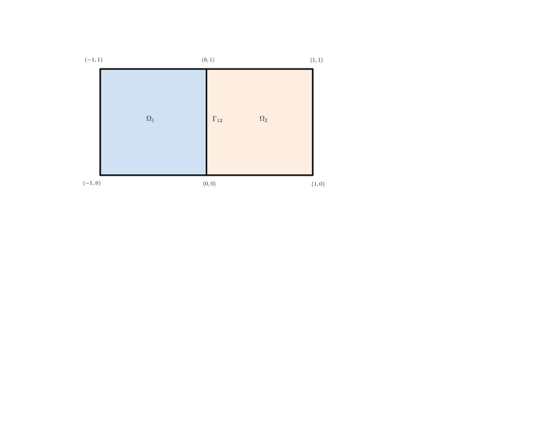
Let and denote the non-overlapping spatial domains , denote the interface and denote a point in . The solution fields and are governed by the following PDE system. ,
| (102) |
with the interface condition
| (103) |
and homogenous Dirichlet boundary conditions on all other boundaries. Figure 1 illustrates the computational domain.
The stochastic diffusion coefficients and are modeled using the following KL expansions. ,
| (104) |
where denotes the mean of and are random variables. Moreover, we assume that has an exponential covariance kernel
| (105) |
where denotes the coefficient of variation and denotes the correlation length of . The analytic expressions for are provided in Appendix A.
The governing PDE system is spatially discretized using bilinear finite elements [34] and equispaced nodes in each subdomain. We therefore obtain linear equations of the form and where are the vectors of nodal values, are the stiffness matrices and denote the respective load vectors. Moreover, the interface condition can also be formulated as the linear equation , where are the interface matrices.
Following the finite element tearing and interconnect (FETI) approach [35], let denote the Lagrange multiplier of the interface equation, , denote the solution variables, and , denote the coupling variables. Subsequently, as per Eq. 2.7, we can formulate a modular algebraic system with following component residuals and interface functions.
| (110) | |||||
| (111) |
The probability density function of the total energy ,
| (112) |
and the statistics of are the quantities of interest in this study. The numerical values of the deterministic parameters used in this study are listed in Table 1.
4.1.2 Modular deterministic solver: Setup and verification
The deterministic solver component and wer developed as function modules, in which the output respective solution updates are computed using Newton’s method as follows.
| (115) | |||
| (116) |
Moreover, to accelerate convergence, a modified relaxed BGS approach was implemented with the optimal value of for both relaxation factors. Subsequently, the second order accuracy of the solver was verified using the method of manufactured solutions (MMS) [36]. Further details are provided in Appendix B.
4.1.3 NISP based uncertainty propagation
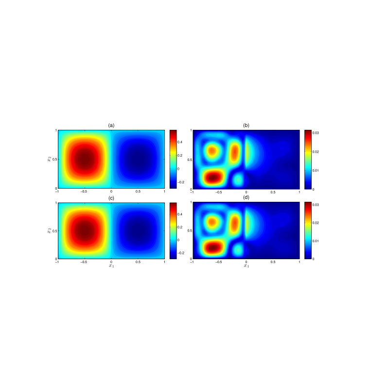
Following the verification study, both the standard and reduced NISP based uncertainty propagation algorithms were implemented by reusing deterministic solver components and . Tolerance values of , , were used in the reduced NISP method implementation. For , , , the probability density function of and the first two solution moments were computed using the converged gPC coefficient matrices and from both algorithms. The results are shown Figure 2 and Figure 3 respectively.

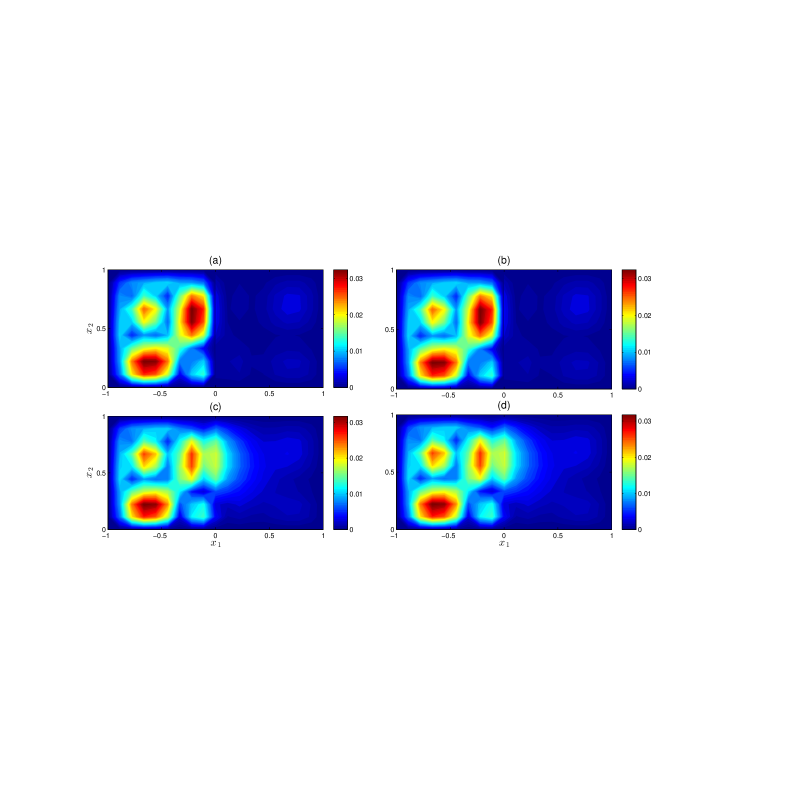
For both algorithms, keeping the mesh size and tolerances values unchanged, the approximation errors and computational costs (wall-times) for several instances of , and are listed in Table 2. Moreover, the parameters of the reduced NISP algorithm in last iteration are also listed. The number of iterations in all tests were observed to be between and in each implementation, which implies that the convergence rate in both algorithms are more or less invariant with respect to the stochastic dimensions , and the order of accuracy . While the choice of the tolerances in the reduced NISP algorithm seem arbitrary, they were in fact selected based on the results of preliminary tests using a coarser mesh. Figure 4 illustratess the effects of varying and on the standard deviation of the solution, for and all other parameters unchanged.
The highest speedup factor observed is . Moreover, the approximation errors in the standard NISP method implementation are observed to decay exponentially, which indicates a high degree of regularity in the stochastic solutions. Furthermore, for the reduced NISP method implementation, the asymptotic upper bound predicted in §3.4, is observed in its approximation errors.
| Standard NISP | Reduced NISP | ||||||||||||
|---|---|---|---|---|---|---|---|---|---|---|---|---|---|
| , | |||||||||||||
.
4.2 Boussinesq flow problem
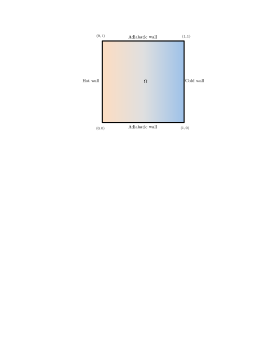
The Boussinesq model describes thermally driven, incompressible flows and is widely used in oceanic and atmospheric modeling [37, 38]. Here, we consider a multi-physics setup with uncertain fluid properties and boundary conditions.
4.2.1 Model setup
Let denote the spatial domain and , denote the non-dimensional [39] fluid velocity, pressure and temperature respectively. The governing equations for the fluid variables are as follows. ,
| (117) | |||||
with homogenous Dirichlet boundary conditions for and Neumann boundary conditions for at all boundaries. The boundary conditions for temperature, as shown in Figure 5, are as follows.
| (118) |
Here, denotes while and denote the Prandtl and Rayleigh numbers respectively. denotes the hot-wall temperature such that ,
| (119) |
where is the mean hot-wall temperature and denotes the perturbation amplitude.
In this study, and are assumed to be independent random fields, and modeled using the following KL expansions. ,
| (120) |
where denotes the mean of and are random variables. Similarly, ,
| (121) |
where are random variables. Moreover, we assume that both and have exponential covariance kernels
| (122) |
where , denote the respective coefficients of variations, and , denote the respective correlation lengths. The analytic expressions for and are provided in Appendix A. Furthermore, the pressure Poisson equation
| (123) |
is used in place of the continuity equation, to close the momentum component of the PDE system.
Each component PDE system is spatially discretized using a finite volume method, with linear central-differencing schemes [40], on a uniform grid with cells. Let denote the respective vectors of cell-centroidal horizontal velocity, vertical velocity, pressure and temperature, which solve the nonlinear system
| (124) |
where each term in Eq. 4.15 denotes its respective discretized operator in the coupled PDE system. Subsequently, we formulate a modular multi-physics setup by separating the momentum and energy components of the coupled algebraic system. As per Eq. 2.5, let , denote the respective solution variables in the modular algebraic system. The component residuals are defined as follows.
| (128) | ||||
| (135) | ||||
| (136) |
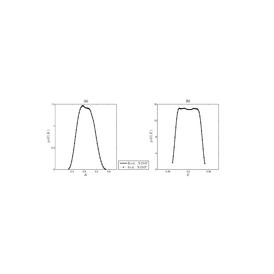
The quantities of interest in this study are the probability density functions of the (scaled) kinetic energy and thermal energy : ,
| (137) |
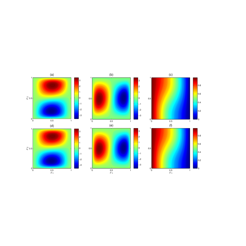
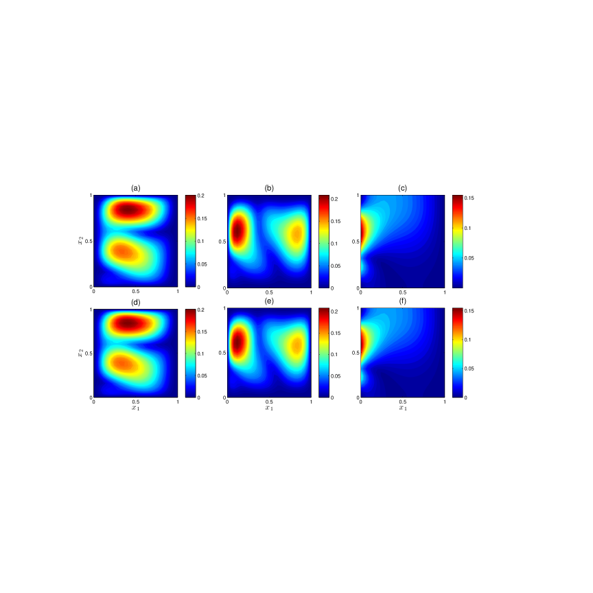
and the statistics of the fluid velocity and temperature. Table 3 lists the numerical values of the deterministic parameters used in this study.
4.2.2 Modular deterministic solver: Setup and verification
The solver components and were developed as function modules, with each module solving a Newton system to compute its respective solution updates. Therefore,
| (138) |
Using MMS, a verification study was carried out and second order accuracy was observed in the numerical solver. The details are provided in Appendix B.
4.2.3 NISP based uncertainty propagation
We implemented both NISP based uncertainty propagation methods by reusing the deterministic solver components and . The tolerance values used in the reduced NISP method implementation are and . Subsequently, for , and , the probability density function of and , and the first two moments of , were computed and compared. The results are shown in Figure 6, Figure 7 and Figure 8 respectively.
| Standard NISP | Reduced NISP | ||||||||||||
|---|---|---|---|---|---|---|---|---|---|---|---|---|---|
For various instances of , and , the approximation errors and computational costs (wall-times) observed in both NISP algorithms, along with the reduced dimensions and orders observed at the last iteration of the reduced NISP algorithm are listed in Table 4. The number of iterations was a constant and equal to for all cases, which once again indicates an invariance of the convergence rate with respect to , and .
Once again, due to the high degree of stochastic regularity exhibited by the solutions, the approximation errors in the standard NISP method implementation are observed to decay exponentially, while the predicted asymptotic upper bound for the approximation errors in the reduced NISP method implementation is observed. The highest speedup factor observed is .
5 Summary and outlook
A reduced NISP based method for uncertainty propagation in stochastic multi-physics models is presented, demonstrated and compared against the standard NISP method using two numerical examples. At the expense of a small approximation error, the reduced NISP method exhibits signifcantly high speedup factors over the standard NISP method. This is primarily due to the much slower growth in the number of repeated runs of each solver component in the former approach, which in turn can be attributed to the dimension and order reduction steps for constructing an approximation of their respective input data. Therefore, the curse of dimensionality, which is the primary bottleneck for any spectral method in tackling large multi-physics models with several independent stochastic components, is demonstrably mitigated with the reduced NISP approach.
In the intermediate dimension reduction step, since the gPC coefficients of the local variables are included in the matrix for which the SVD is computed, we the local stochastic dimension in each module would serve as a lower bound for the respective reduced dimension. This suggests that the modular structure of the stochastic solver enables our proposed reduction strategy, which would fail to provide a reduced approximation if implemented with a fully-coupled (monolithic) NISP solver. The lower bound on the reduced dimension can also be observed in the numerical experiments.
The two most significant overheads observed while implementing the reduced NISP algorithm were the computation of the Vandermonde matrix for the construction of the reduced quadrature rule, and the computation of the global gPC coefficient matrices from the reduced gPC coefficient matrices. Both these overheads can be easily eliminated due to the embarrassingly parallel nature of the computations involved. Moreover, in each numerical example, both the NISP algorithms were implemented using a sparse grid global quadrature rule. If a full tensor grid were used, the computational gains observed in the reduced NISP method implementation would be much higher. Furthermore, alternatives, for example, Schur complement based elimination, to the BGS partitioning approach can be explored for reducing the overall computational costs.
The applicability of our proposed algorithm is limited to models in which the global stochastic dimension is manageably low (), since the global gPC coefficients still need to be computed, stored and operated on. If the global stochastic dimension becomes prohibitively large due to a particular module contributing a large number of independent uncertainties, a Monte-Carlo based sampling approach can be employed in that module, while other modules could still afford the use of spectral methods. Such a framework has been recently demonstrated in [41], and further explorations to develop a more general approach are currently underway. Moreover, for tackling models in which the solution regularity is low, the proposed method can also be easily adapted towards multi-element gPC [42] and discontinuous wavelet [43] based spectral representations.
Extending the framework of dimension and order reduction to intrusive spectral projection (ISP)- based uncertainty propagation would be particularly important in mitigating the overall intrusiveness and therefore, development costs incurred by the solver modules. Moreover, derivative or active-subspace based dimension reduction methods [44] have provided potential alternative approaches which are not yet fully explored. Futhermore, the additional complexities and approximation errors that arise in tackling unsteady multi-physics models using spectral methods have led to several challenges and opportunities for improvement.
Acknowledgement
This research was funded by the US Department of Energy, Office of Advanced Computing Research and Applied Mathematics Program and partially funded by the US Department of Energy NNSA ASC Program.
References
- [1] G. Casella and C. Robert, Monte Carlo statistical methods, Springer, New York, 1999.
- [2] P. Glasserman, Quasi-Monte Carlo, Monte Carlo Methods in Financial Engineering, Springer, New York, 2003, pp. 281-337.
- [3] H. Rauhut and R. Ward, Sparse Legendre expansions via 1-minimization, J. Approx. Theory, 164.5 (2012), pp. 517-533.
- [4] J. Peng, J. Hampton, and A. Doostan, A weighted 1-minimization approach for sparse polynomial chaos expansions, J. Comput. Phys., 267 (2014), pp. 92-111.
- [5] K. Park, C. Carlos, A. Felippa and R. Ohayon, Partitioned formulation of internal fluid–structure interaction problems by localized Lagrange multipliers, Computer Methods Appl. Mech. Engrg., 190.24 (2001), pp. 2989-3007.
- [6] J. Kanney, C. Miller and C. T. Kelley, Convergence of iterative split-operator approaches for approximating nonlinear reactive transport problems, Advances in Water Resources, 26.3 (2003), pp. 247-261.
- [7] D. Luenberger and Y. Ye, Linear and nonlinear programming. Springer, New York, 2008.
- [8] D. Xiu and G. Karniadakis, Modeling uncertainty in flow simulations via generalized polynomial chaos, J. Comput. Phys., 187.1 (2003), pp. 137-167.
- [9] P. Constantine, A. Doostan and G. Iaccarino, A hybrid collocation/Galerkin scheme for convective heat transfer problems with stochastic boundary conditions, International Journal for Numerical Methods in Engineering, 80.7 (2009), pp. 868-880.
- [10] X. Chen, B. Ng, Y. Sun and C. Tong, A flexible uncertainty quantification method for linearly coupled multi-physics systems, J. Comput. Phys., Physics 248 (2013), pp. 383-401.
- [11] X. Chen, B. Ng, Y. Sun and C. Tong, A computational method for simulating subsurface flow and reactive transport in heterogeneous porous media embedded with flexible uncertainty quantification, Water Resources Research, 49 (2013), pp. 5740-5755.
- [12] M. Hadigol, A. Doostan, H. Matthies and R. Niekamp, Partitioned treatment of uncertainty in coupled domain problems: A separated representation approach, Computer Methods Appl. Mech. Engrg., 274 (2014), pp. 103-124.
- [13] P. Constantine, E. Phipps and T. Wildey, Efficient uncertainty propagation for network multi-physics systems, International Journal for Numerical Methods in Engineering, (2014).
- [14] M. Arnst, R. Ghanem, E. Phipps and J. Red-Horse, Measure transformation and efficient quadrature in reduced-dimensional stochastic modeling of coupled problems, International Journal for Numerical Methods in Engineering, 92 (2012), pp. 1044-1080.
- [15] M. Arnst, R. Ghanem, E. Phipps and J. Red-Horse, Reduced chaos expansions with random coefficientsin reduced-dimensional stochastic modeling of coupled problems, International Journal for Numerical Methods in Engineering, 97 (2014), pp. 352-376.
- [16] C. Soize and R. Ghanem, Reduced chaos decomposition with random coefficients of vector-valued random variables and random fields, Computer Methods Appl. Mech. Engrg., 198 (2009), pp. 1926-1934.
- [17] C. Broyden, A class of methods for solving nonlinear simultaneous equations, Math. Comp., (1965), pp. 577-593.
- [18] H. Hartley, The modified Gauss-Newton method for the fitting of non-linear regression functions by least squares, Technometrics, 3 (1961), pp. 269-280.
- [19] J. More, The Levenberg-Marquardt algorithm: implementation and theory, in Numerical analysis, Springer, Heidelberg, 1978, pp. 105-116.
- [20] H. Matthies, R. Niekamp and J. Steindorf, Algorithms for strong coupling procedures. Computer Methods Appl. Mech. Engrg., 195 (2006), pp. 2028-2049.
- [21] P. Davis, Interpolation and approximation, Dover Publications, 1975.
- [22] W. Gautschi, Orthogonal polynomials: applications and computation, Acta Numer., 5 (1996), pp. 45-119.
- [23] W. Gautschi, On generating orthogonal polynomials, SIAM J. Sci. Comp., 3 (1982), pp. 289-317.
- [24] R. Cameron and W. Martin, The orthogonal development of non-linear functionals in series of Fourier-Hermite functionals, Ann. of Math., (1947), pp. 385-392.
- [25] B. Silverman, Density estimation for statistics and data analysis,, CRC press, 1986.
- [26] M. Reagana, H. Najm, R. Ghanem and O. Knio, Uncertainty quantification in reacting-flow simulations through non-intrusive spectral projection, Combustion and Flame, 132 (2003), pp. 545-555.
- [27] F. Nobile, Fabio, R. Tempone and C. Webster, A sparse grid stochastic collocation method for partial differential equations with random input data, SIAM J. Numer. Anal., 46 (2008), pp. 2309-2345.
- [28] M. Loeve, Probability Theory. Foundations. Random Sequences,, D. Van Nostrand Company, New York, 1955.
- [29] K. Petersen and M. Pedersen, The matrix cookbook, Technical University of Denmark, (2008), pp. 7-15.
- [30] J. Nelder and R. Mead, A simplex method for function minimization, The Computer Journal, 7 (1965), pp. 308-313.
- [31] V. Tchakaloff, Formules de cubatures mécaniquesa coefficients non négatifs, Bull. Sci. Math., 81 (1957), pp. 123-134.
- [32] P. Constantine, D. Gleich and G. Iaccarino, Spectral methods for parameterized matrix equations, SIAM J. Matrix Anal. Appl., 31 (2010), pp. 2681-2699.
- [33] D. Xiu and J. Hesthaven, High-order collocation methods for differential equations with random inputs, SIAM J. Sci. Comp., 27 (2005), pp. 1118-1139.
- [34] T. Hughes, The finite element method: linear static and dynamic finite element analysis,, Dover Publications, 2012.
- [35] C. Farhat, J. Mandel and F. Roux, Optimal convergence properties of the FETI domain decomposition method, Computer methods Appl. Mech. Engrg., 115 (1994), pp. 365-385.
- [36] P. Roache, Code verification by the method of manufactured solutions, Journal of Fluids Engineering, 124 (2002), pp. 4-10.
- [37] L. Kantha and C. Clayson, Numerical models of oceans and oceanic processes, Academic press, 2000.
- [38] J. Massaguer and J. Zahn, Cellular convection in a stratified atmosphere, Astronom. and Astrophys. Lib., 87 (1980), pp. 315-327.
- [39] D. de Vahl, Laminar natural convection in an enclosed rectangular cavity, International Journal of Heat and Mass Transfer, 11 (1968), pp. 1675-1693.
- [40] R. LeVeque, Finite volume methods for hyperbolic problems, Cambridge University Press, 2002.
- [41] M. Arnst, C. Soize and R. Ghanem, A Hybrid Sampling/Spectral Method for Solving Stochastic Coupled Problems, SIAM Journal on Uncertainty Quantification, (2013), pp. 218-243.
- [42] X. Wan and G. Karniadakis, Multi-element generalized polynomial chaos for arbitrary probability measures, SIAM J. Sci. Comp., 28 (2006), pp. 901-928.
- [43] O Le Maitre, O. Knio, H. Najm, and R. Ghanem, Uncertainty propagation using Wiener-Haar expansions, J. Comput. Phys., 197 (2004), pp. 28-57.
- [44] T. Lukaczyk, F. Palacios, J. Alonso and P. Constantine, Active Subspaces for Shape Optimization, 10th AIAA Multidisciplinary Design Optimization Conference, Maryland, 2014.
Appendix A - Karhunen-Loeve expansion
Exponential covariance kernel
Given an -dimensional spatial domain , let denote the exponential covariance kernel of a spatially varying random field . Therefore, ,
| (A.1) |
where denotes the correlation length. Subsequently, we can define the KL expansion of using an infinite set of random variables , each having zero mean and unit variance, as follows. ,
Appendix B - Verification of modular solvers
B1 - Poisson problem
Given stochastic diffusion coefficients and , we choose analytical functions , ,
| (B.1) |
which solve the modified coupled-domain Poisson equations:,
| (B.2) |
Here, ,
| (B.3) |
If denote the corresponding finite element solutions obtained using nodes, then ,
| (B.4) |
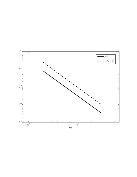
denotes the mean-square error at discretization level . We used a tolerance and set the the stochastic dimensions to . Subsequently, for different values of , we computed the sample average of , denoted here as , using Monte-Carlo solution samples. Figure B1 illustrates the expected second order rate of decay in .
B2 - Boussinesq flow problem
Following the same procedure in Appendix B1, we choose analytical functions ,
| (B.5) |
which solve the modified Boussinesq equations: ,
| (B.6) | ||||
Here, ,
| (B.7) |
Let ,
denote the mean-square error between the exact and approximate solutions , computed using cells.
Subsequently, the average error , was computed using 100 Monte-Carlo samples for various values of , shown in Figure B2, keeping the tolerance at and stochastic dimensions to . As expected, a second order rate of decay rate is observed in .

