Dirac Reduction for Nonholonomic Mechanical Systems and Semidirect Products

Abstract

This paper develops the theory of Dirac reduction by symmetry for nonholonomic systems on Lie groups with broken symmetry. The reduction is carried out for the Dirac structures, as well as for the associated Lagrange-Dirac and Hamilton-Dirac dynamical systems. This reduction procedure is accompanied by reduction of the associated variational structures on both Lagrangian and Hamiltonian sides. The reduced dynamical systems obtained are called the implicit Euler-Poincaré-Suslov equations with advected parameters and the implicit Lie-Poisson-Suslov equations with advected parameters. The theory is illustrated with the help of finite and infinite dimensional examples. It is shown that equations of motion for second order Rivlin-Ericksen fluids can be formulated as an infinite dimensional nonholonomic system in the framework of the present paper.

keywords:

Dirac structures, reduction by symmetry, nonholonomic systems, variational structures, semidirect products, Rivlin-Ericksen fluids. 2010 Mathematics Subject Classification. 70H30, 70H45, 70H03, 70H05, 37J60.

Contents

1. 1 Introduction
2. 2 Dirac dynamical systems
   1. 2.1 Lagrange-d’Alembert-Pontryagin principle
   2. 2.2 Hamilton-d’Alembert phase space principle
   3. 2.3 Dirac dynamical systems
   4. 2.4 Lie-Dirac reduction
   5. 2.5 Euler-Poincaré-Dirac reduction
   6. 2.6 Lie-Poisson-Dirac reduction
3. 3 Semidirect product theory
   1. 3.1 Euler-Poincaré reduction with advected parameters
   2. 3.2 Lie-Poisson reduction on semidirect products
4. 4 Variational framework
   1. 4.1 The unconstrained case
   2. 4.2 The case of systems with nonholonomic constraints
   3. 4.3 Rolling ball type constraints on semidirect products
   4. 4.4 Generalization to arbitrary advected quantities
   5. 4.5 Variational framework on the Hamiltonian side
5. 5 Lie-Dirac reduction with advected quantities
   1. 5.1 Lie-Dirac reduction of the induced Dirac structures
   2. 5.2 Euler-Poincaré-Dirac reduction with advected parameters
   3. 5.3 Preliminary comments on the Hamilton-Dirac reduction
6. 6 Lie-Dirac reduction for nonholonomic systems on semidirect products
   1. 6.1 Lie-Dirac reduction: a more general case
   2. 6.2 Lie-Dirac reduction by stages on semidirect products
   3. 6.3 Relation with the Lagrange-Dirac side
   4. 6.4 The Hamilton-d’Alembert principle in phase space
   5. 6.5 Dirac reduction for rolling ball type constraints on semidirect products
7. 7 Examples
   1. 7.1 The heavy top
   2. 7.2 Incompressible ideal fluids
   3. 7.3 Compressible MHD
   4. 7.4 The Chaplygin rolling ball
   5. 7.5 The Euler disk
   6. 7.6 Second-order Rivlin-Ericksen fluids

1 Introduction

Dirac structures in mechanics.

Dirac structures are geometric objects that generalize both Poisson brackets and (pre)symplectic structures on manifolds. They were originally developed by Courant, Weinstein [1988]; Courant [1990] and Dorfman [1993] and were named after Dirac’s theory of constraints (Dirac [1950]).

It turns out that Dirac structures are the appropriate geometric objects for the formulation of equations of motion of nonholonomic Hamiltonian systems on arbitrary configuration manifolds or, more generally, of implicit Hamiltonian systems appearing as differential-algebraic equations (see, for instance, van der Schaft, Maschke [1995] and Bloch, Crouch [1997]). More recently, the notion of an implicit Lagrangian system, which may be a Lagrangian analogue of an implicit Hamiltonian system, was developed by Yoshimura, Marsden [2006a], where it was shown that nonholonomic mechanical systems and L-C circuits can be formulated as degenerate Lagrangian systems in this context.

For the case of nonholonomic mechanics, given a constraint distribution $\Delta_{Q}$ on the configuration manifold $Q$, there exists an associated Dirac structure $D_{\Delta_{Q}}$ on the cotangent bundle $T^{*}Q$ of $Q$, introduced in Yoshimura, Marsden [2006a]. This Dirac structure is not integrable, unless the constraint is holonomic. Given such an induced Dirac structure and a (possibly degenerate) Lagrangian defined on the tangent bundle $TQ$ of $Q$, a Lagrange-Dirac dynamical system can be defined (Yoshimura, Marsden [2006a]), which provides a geometric formulation of the equations of motion for the nonholonomic mechanical systems. The associated equations of motion are the so-called implicit Lagrange-d’Alembert equations. The Lagrange-Dirac system is naturally associated to a variational structure, called the Lagrange-d’Alembert-Pontryagin principle whose critical curves are precisely the solutions of the implicit Lagrange-d’Alembert equations.

On the Hamiltonian side, dynamical systems associated to Dirac structures were considered in Dorfman [1987]; Courant, Weinstein [1988] and Courant [1990]. Further applications of Dirac structures to dynamical systems including L-C circuits and nonholonomic systems were developed by van der Schaft, Maschke [1995] and Bloch, Crouch [1997]. The case of the Dirac structure $D_{\Delta_{Q}}$ induced by a nonholonomic constraint $\Delta_{Q}\subset TQ$ was considered in Yoshimura, Marsden [2007b] to formulate a Hamilton-Dirac system in nonholonomic mechanics.

In the presence of symmetries, there is a well-developed reduction theory for Dirac structures in mechanics for $G$-invariant systems on Lie groups, both in the unconstrained case and in the constrained (nonintegrable) case (Yoshimura, Marsden [2007b]), where the associated Dirac reduction process (called Lie-Dirac reduction) yields the geometric framework for the study of the Euler-Poincaré-Suslov and Lie-Poisson-Suslov equations. For the more general case of a free and proper Lie group action on an arbitrary configuration manifold, a reduction theory called Dirac cotangent bundle reduction was developed for the canonical Dirac structure (Yoshimura, Marsden [2009]). It induces the implicit Lagrange-Poincaré equations on the Lagrangian side and the implicit Hamilton-Poincaré equations on the Hamiltonian side. Note that this process of Dirac reduction does not only provide a geometric setting for the reduction of the equations of motion (both on the Lagrangian and Hamiltonian case), but also allows for a corresponding reduction of the associated variational structures.

Other Dirac reduction processes have been developed by Courant [1990], Dorfman [1993], Blankenstein, van der Schaft [2001] and Bursztyn, Cavalcanti, Gualtieri [2007].

Lagrangian reduction for holonomic mechanical systems on Lie groups.

From the viewpoint of reduction by symmetries in Lagrangian systems, the simplest situation arises when the configuration manifold coincides with the Lie group of symmetries. This is the well-known situation of the Euler-Poincaré reduction whose main examples are rigid bodies and incompressible fluids, and this allows to reformulate the Euler-Lagrange equation on the Lie group as a first-order differential equation on the Lie algebra (see, for instance, Marsden, Ratiu [1999]).

In many relevant situations in physics, however, the symmetry of the system is broken by the presence of a parameter held fixed in the Lagrangian description, i.e., before reduction.

After reduction (i.e., in the convective or spatial description) this parameter becomes time dependent and verifies an advection equation; hence it was named Euler-Poincaré reduction with advected parameters for the associated reduction process. It has been developed in Holm, Marsden, Ratiu [1998] and applied there to several examples such as heavy tops, compressible fluids and magnetohydrodynamics. The Hamiltonian formulation of the Euler-Poincaré reduction with advected parameters can be related to the earlier derived Lie-Poisson reduction on semidirect products of Marsden, Ratiu, Weinstein [1984]. It is useful to mention that, on the Lagrangian side, the Euler-Poincaré equations with advected parameters are not the Euler-Poincaré equations on a semidirect product. Such a comment is crucial for the Dirac formulation that we will develop subsequently in the paper.

Physical systems with advected parameters can be also approached by using the general methods of Lagrangian reduction in Cendra, Ibort, Marsden [1987] and Cendra, Marsden, Ratiu [2001].

Recently, several generalizations of Euler-Poincaré reduction with advection have been made in order to treat the case of complex fluids (Gay-Balmaz, Ratiu [2009]), nonabelian charged fluids (Gay-Balmaz, Ratiu [2011]), rods and molecular strands (Gay-Balmaz, Holm, Ratiu [2009], Ellis, Gay-Balmaz, Holm, Putkaradze, Ratiu [2010]), or nematic systems with broken symmetry (Gay-Balmaz, Tronci [2010]).

Lagrangian reduction for nonholonomic systems.

One of the first paper in which a systematic theory of nonholonomic reduction is developed is Koiller [1992]. A Hamiltonian version of this theory was developed in Bates, Sniatycki [1993], while a Lagrangian version was given in Bloch, Krishnaprasad, Marsden, Murray [1996]. Links between these theories and further developments were given in Koon, Marsden [1997, 1998]. The intrinsic geometric formulation of the Lagrangian reduction theory for nonholonomic systems was given in Cendra, Marsden, Ratiu [2001]. An application of this reduction theory to the Euler disk was carried out in Cendra, Diaz [2007], from which a geometric integrator was derived in Campos, Cendra, Diaz, Martin de Diego [2012]. Reduction for nonholonomic systems was generalized to the setting of Lie algebroids in Cortes, de Leon, Marrero, Martinez [2009].

Nonholonomic Lagrangian reduction for systems with broken symmetry on Lie groups has not been developed yet and a part of our present work is dedicated to this task, besides the development of the Hamilton-Pontryagin variational formulation and the associated Dirac reduction. The closest relevant work in this direction is Schneider [2002], in which nonholonomic Euler-Poincaré reduction was developed in a particular setting well appropriate for several examples of rigid bodies that roll without slipping. Besides the classical examples of rigid bodies with nonholonomic constraints, the nonholonomic reduction that we develop is also motivated from the work of Gay-Balmaz, Putkaradze [2012, 2014] on the dynamics of elastic strings with rolling contact.

Goal of the paper.

The main goal of this paper is to develop the reduction theory of Dirac structures for holonomic and nonholonomic systems on Lie groups with broken symmetry. This concerns the reduction of Dirac structures as a geometric object, together with the reduction of the associated Lagrange-Dirac and Hamilton-Dirac dynamical systems, as well as the associated variational structures on both the Lagrangian and Hamiltonian sides.

The reduction process for these systems with advected parameters is carried out by considering a parameter dependent constraint $\Delta^{a_{0}}_{G}$ on a Lie group $G$, where the parameter $a_{0}$ belongs to the vector space of advected parameters on which the group is assumed to act by representation. Under the appropriate invariance of both a Lagrangian and constraints under the isotropy subgroup $G_{a_{0}}$ of $a_{0}$, we derive the reduced equations of motion (called implicit Euler-Poincaré-Suslov equations with advected parameters) via the Lagrange-d’Alembert-Pontryagin principle, and with their Hamiltonian version via the Hamilton-d’Alembert principle. This approach is then developed in the context of Dirac geometry, by considering the parameter dependent Dirac structure $D_{\Delta^{a_{0}}_{G}}$ on $T^{*}G$ associated to the constraint $\Delta^{a_{0}}_{G}$ and its reduction by the isotropy subgroup $G_{a_{0}}$. From the viewpoint of dynamics, this allows us to formulate the reduction of the associated Lagrange-Dirac and Hamilton-Dirac systems and also to show that they provide the appropriate geometric framework for the formulation of the Euler-Poincaré-Suslov equations with advected parameters and its Hamiltonian version. In particular, we show that, on the Hamiltonian side, the Dirac reduction can be interpreted as the second step of a Dirac reduction by stages for semidirect products, thereby extending the whole existing holonomic reduction theory for semidirect products to the context of the Dirac reduction for nonholonomic mechanics.

Outline of the paper.

The paper is organized as follows. In Section 2, we introduce the required mathematical ingredients for Dirac structures in mechanics and the associated variational structures. We first recall the Lagrange-d’Alembert-Pontryagin principle and the Hamilton-d’Alembert principle for nonholonomic mechanics, together with their reduced versions on Lie groups. Then, we review the definition of Dirac structures, mention the Dirac structure induced from a constraint set, and recall the definitions of Lagrange-Dirac and Hamilton-Dirac dynamical systems. Thus, we explain the reduction of Dirac structures associated with the invariant constraints on Lie groups (the so-called Lie-Dirac reduction), and the reduction of the corresponding Lagrange-Dirac and Hamilton-Dirac systems (the so-called Euler-Poincaré-Dirac and Lie-Poisson-Dirac reductions). In Section 3, we review the theory of (holonomic) Euler-Poincaré reduction with advected quantities together with its Hamiltonian analogue. In particular, we recall that on the Hamiltonian side the reduction process can be interpreted as the second stage of the ordinary Lie-Poisson reduction for a semidirect product. In Section 4, we first present the Hamilton-Pontryagin principle and its reduced version for holonomic systems on Lie groups with advected quantities. Then we extend this principle to the case of nonholonomic systems, thereby obtaining the implicit Euler-Poincaré-Suslov equations with advected quantities. We also carry out reduction of the variational structure to obtain the implicit Lie-Poisson-Suslov equations with advected parameters on the Hamiltonian side. Thus, we treat an important class of constraints appearing in several examples of nonholonomic rigid bodies, when the Lie group configuration space is a semidirect product. In Section 5, we carry out the reduction of Dirac structures associated to a parameter dependent nonholonomic constraint on a Lie group, and the reduction of the corresponding Lagrange-Dirac and Hamilton-Dirac dynamical systems. We show that these reduced systems are equivalent to the implicit Euler-Poincaré-Suslov equations with advected parameter and their Hamiltonian version. We also note that, on the Hamiltonian side, the Dirac reduction theory developed so far does only parallel partially the holonomic situation, which can be interpreted as the second stage reduction of a Lie-Poisson reduction for semidirect products. This discrepancy is solved in Section 6, where it is shown that a Dirac reduction by stages for semidirect products can be carried out for nonholonomic systems with advected quantities. The associated variational structures are explained. Finally in Section 7 we consider several examples that illustrate our theory, such as the heavy top, the incompressible ideal fluid and MHD, the Chaplygin ball, and the Euler disk. We show that the equations of motion for the second order Rivlin-Ericksen fluids is a nonholonomic system in the framework of the theory developed in the present paper.

2 Dirac dynamical systems

This section contains an extended review of Dirac dynamical systems and the associated variational structures as required mathematical ingredients in this paper. We first recall the expression of the Lagrange-d’Alembert-Pontryagin principle and the Hamilton-d’Alembert principle, both for the unconstrained and constrained cases. In the special situation in which the configuration manifold is a Lie group, we review the reduced version of these variational structures. We then recall the definition of Dirac structures and the associated dynamical systems, both on the Lagrangian and Hamiltonian sides, together with the associated reduction procedures called Lie-Dirac reduction on a Lie group configuration space.

2.1 Lagrange-d’Alembert-Pontryagin principle

Let $Q$ be a manifold thought of as the configuration space of a mechanical system. We denote by $TQ\rightarrow Q$, $T^{*}Q\rightarrow Q$, and $TQ\oplus T^{\ast}Q\rightarrow Q$, the tangent bundle, the cotangent bundle, and the Pontryagin bundle, respectively, with local coordinates $(q,v)\in TQ$, $(q,p)\in T^{\ast}Q$, and $(q,v,p)\in TQ\oplus T^{\ast}Q$. Let $\Delta_{Q}\subset TQ$ be a smooth constraint distribution on $Q$. Let $L:TQ\to\mathbb{R}$ be the (possibly degenerate) Lagrangian of the system.

The Lagrange-d’Alembert-Pontryagin principle is

$$\delta\int_{t_{1}}^{t_{2}}\left\{L(q(t),v(t))+\left\langle p(t),\dot{q}(t)-v(t)\right\rangle\right\}\,dt=0,$$ (2.1)

where $v$ has to satisfy the constraint $v(t)\in\Delta_{Q}(q(t))$ and for variations $(\delta q(t),\delta v(t),\delta p(t))$ of the curves $(q(t),v(t),p(t))$ such that $\delta q(t)\in\Delta_{Q}(q(t))$ and vanishes at the endpoints. The stationarity conditions yield the equations, in local coordinates,

$$\begin{split}p=\frac{\partial L}{\partial v},\quad\dot{q}=v\in\Delta_{Q}(q),\quad\dot{p}-\frac{\partial L}{\partial q}\in\Delta_{Q}(q)^{\circ},\end{split}$$

called the implicit Lagrange-d’Alembert equations on $TQ\oplus T^{\ast}Q$; see Yoshimura, Marsden [2006b].

Note that the implicit Lagrange-d’Alembert equations include the Lagrange-d’Alembert equations $\dot{p}-{\partial L}/{\partial q}\in\Delta_{Q}(q)^{\circ}$, the Legendre transformation $p={\partial L}/{\partial v}$ and the second–order condition $\dot{q}=v\in\Delta_{Q}(q)$.

In the unconstrained case $\Delta_{Q}=TQ$, the principle (2.1) is called the Hamilton-Pontryagin principle and it recovers the implicit Euler-Lagrange equations.

Reduction on Lie groups.

When the Lagrangian is invariant under the tangent lifted action of a Lie group $G$ on the configuration manifold $Q$, one can reduce both the equations and the variational structure. We shall focus on the case when $Q=G$ and $G$ acts by left translation. As a consequence, the group $G$ acts on curves $(g(t),v(t),p(t))$ in $TG\oplus T^{\ast}G$ by simultaneously left translating on each factor by the left-action and its tangent and cotangent lifts, i.e., the action of $h\in G$ is

$$h\cdot(g(t),v(t),p(t)):=(hg(t),T_{g(t)}L_{h}\cdot v(t),T^{\ast}_{hg(t)}L_{h^{-1}}\cdot p(t))=:(hg(t),hv(t),hp(t)),$$

where $T_{g(t)}L_{h}:T_{g(t)}G\to T_{hg(t)}G$ is the tangent of the left translation map $L_{h}:G\to G;\,g(t)\mapsto hg(t)$ at the point $g(t)$ and $T^{\ast}_{hg(t)}L_{h^{-1}}:T^{\ast}_{g(t)}G\to T^{\ast}_{hg(t)}G$ is the dual of the map $T_{hg(t)}L_{h^{-1}}:T_{hg(t)}G\to T_{g(t)}G$.

Let us assume that the constraint distribution $\Delta_{G}\subset TG$ on $G$ is left invariant under the group action $g\mapsto hg$, which means that for all $h\in G$, the subspace $\Delta_{G}(g)\subset T_{g}G$ is mapped by the tangent map of the group action to the subspace $\Delta_{G}(hg)\subset T_{hg}G$, that is

$$\Delta_{G}(hg)=h\Delta_{G}(g),\quad\text{for all $h\in G$}.$$ (2.2)

By $G$-invariance, $\Delta_{G}$ is completely determined by its value at the identity, namely, by the vector subspace $\mathfrak{g}^{\Delta}:=\Delta_{G}(e)\subset\mathfrak{g}$.

Let $L:TG\rightarrow\mathbb{R}$ be a $G$-invariant Lagrangian and let $\ell:\mathfrak{g}\to\mathbb{R}$ given by $\ell:=L|{\mathfrak{g}}$ be the reduced Lagrangian.

The Lagrange-d’Alembert-Pontryagin action integral is invariant under the action of $G$ since $L$ is $G$–invariant and one easily checks that $\langle p(t),\dot{g}(t)-v(t)\rangle$ is also $G$-invariant. The reduced Lagrange-d’Alembert-Pontryagin principle for nonholonomic mechanics is given by

$$\delta\int_{t_{0}}^{t_{1}}\left\{\ell(\eta)+\left\langle\mu,\xi-\eta\right\rangle\right\}dt=0,\quad\delta{\xi}=\frac{\partial\zeta}{\partial t}+[\xi,\zeta],\quad\text{where}\quad\zeta\in\mathfrak{g}^{\Delta},\quad\eta\in\mathfrak{g}^{\Delta},$$ (2.3)

which yields the implicit Euler-Poincaré-Suslov equations on $(\mathfrak{g}\oplus\mathfrak{g}^{\ast})\times V^{\ast}$:

$$\mu=\frac{\delta\ell}{\delta\eta},\quad\xi=\eta\in\mathfrak{g}^{\Delta},\quad\dot{\mu}-\operatorname{ad}_{\xi}^{\;\ast}\mu\in\left(\mathfrak{g}^{\Delta}\right)^{\circ}.$$ (2.4)

This approach was developed by Yoshimura, Marsden [2007b] and is the implicit analogue of the Euler-Poincaré-Suslov theory. We refer to Kozlov [1988] and Bloch [2003] for the details on the original Suslov problem and its generalization.

Remark 2.1 (Alternative formulation of the Hamilton-Pontryagin principle).

For the unconstrained case, a similar variational principle to the one given in the above was also considered in Bou-Rabee, Marsden [2009]. It reads

$$\delta\int_{t_{1}}^{t_{2}}\{\ell(\xi)+\left\langle\mu,g^{-1}\dot{g}-\xi\right\rangle\}\,dt=0,$$ (2.5)

for arbitrary variations $(\delta\xi(t),\delta\mu(t))$ of $(\xi(t),\mu(t))\in\mathfrak{g}\oplus\mathfrak{g}^{\ast}$ and variations $\delta g(t)$ of $g(t)\in G$ vanishing at the endpoints and yields the stationarity conditions

$$\xi=g^{-1}\dot{g},\quad\mu=\frac{\delta\ell}{\delta\xi},\quad\dot{\mu}-\operatorname{ad}^{\ast}_{\xi}\mu=0.$$

Note that this variational principle in $G\times\mathfrak{g}\oplus\mathfrak{g}^{\ast}$ can be understood as the trivialized expression of the Hamilton-Pontryagin principle on $TG\oplus T^{\ast}G$. As opposed to the reduced Hamilton-Pontryagin principle (that is (2.3) without constraints), the Hamilton-Pontryagin principle (2.5) still contains the unreduced variables $g,\dot{g}$, and is therefore not the reduced expression of the Hamilton-Pontryagin principle on $TG\oplus T^{*}G$. However, it may have the advantage of involving only unconstrained variations, for instance, in the case of numerical integrations. Of course, both variational principles yield equivalent equations.

2.2 Hamilton-d’Alembert phase space principle

Let $H:T^{\ast}Q\rightarrow\mathbb{R}$ be a Hamiltonian function defined on the cotangent bundle (phase space) of the configuration manifold $Q$. In presence of a smooth distribution constraint $\Delta_{Q}\subset TQ$, the equations of motions are obtained by the Hamilton-d’Alembert principle in phase space

$$\delta\int\left\{\left\langle p(t),\dot{q}(t)\right\rangle-H(q(t),p(t))\right\}dt=0,$$

where $\dot{q}(t)\in\Delta_{Q}(q(t))$, and for variations $\delta q(t),\delta p(t)$ such that $\delta q(t)\in\Delta_{Q}(q(t))$ and vanishes at the endpoints; see Yoshimura, Marsden [2006b]. This principle yields the Hamilton-d’Alembert equations for nonholonomic mechanics:

$$\dot{q}=\frac{\partial H}{\partial p}\in\Delta_{Q},\quad\frac{\partial H}{\partial q}+\dot{p}\in\Delta^{\circ}_{Q}.$$

We refer to Bates, Sniatycki [1993], van der Schaft, Maschke [1995] and Marle [1998], for the description of geometric formalisms for Hamiltonian systems with nonholonomic constraints.

Reduction on Lie groups.

Let us consider the case $Q=G$, with $G$ acting on the left by translations and assume that the given distribution $\Delta_{G}$ on $G$ is left-invariant.

Let $H$ be a $G$-invariant Hamiltonian on $T^{\ast}G$ and let $h:\mathfrak{g}^{\ast}\rightarrow\mathbb{R}$ given by $h:=H|_{\mathfrak{g}^{\ast}}$ be the reduced Hamiltonian. The reduced Hamilton-d’Alembert principle is given by

$$\delta\int_{t_{1}}^{t_{2}}\left\{\left\langle\mu,\xi\right\rangle-h(\mu)\right\}dt=0,$$

for $\xi\in\mathfrak{g}^{\Delta}$ and with the variations of the form

$$\delta{\xi}=\frac{\partial\zeta}{\partial t}+[\xi,\zeta].$$

This principle yields the implicit Lie-Poisson-Suslov equations for nonholonomic mechanics:

$$\dot{\mu}-\operatorname{ad}^{*}_{\xi}\mu\in(\mathfrak{g}^{\Delta})^{\circ}\quad\text{and}\quad\frac{\delta h}{\delta\mu}=\xi\in\mathfrak{g}^{\Delta}.$$

For the unconstrained case, this principle is called the Lie-Poisson variational principle (see Cendra, Marsden, Pekarski, Ratiu [2003]) and it yields the implicit Lie-Poisson equations

$$\frac{\delta h}{\delta\mu}=\xi,\quad\dot{\mu}-\operatorname{ad}^{\ast}_{\xi}\mu=0.$$

Remark 2.2 (Alternative formulation of the Lie-Poisson variational principle).

As before, one can develop the trivialized Hamilton principle in phase space as

$$\delta\int_{t_{1}}^{t_{2}}\{\left\langle\mu,g^{-1}\dot{g}\right\rangle-h(\mu)\}\,dt=0,$$

for arbitrary variations $\delta\mu(t)$ of $\mu(t)\in\mathfrak{g}^{\ast}$ and variations $\delta g(t)$ of $g(t)\in G$ vanishing at the endpoints. It yields the stationarity conditions

$$g^{-1}\dot{g}=\frac{\delta h}{\delta\xi},\quad\dot{\mu}=\operatorname{ad}^{\ast}_{g^{-1}\dot{g}}\mu.$$

2.3 Dirac dynamical systems

Linear Dirac structures.

We first recall the definition of a Dirac structure on a vector space $V$, see Courant, Weinstein [1988]. Let $V^{\ast}$ be the dual space of $V$, and $\langle\cdot\,,\cdot\rangle$ be the natural paring between $V^{\ast}$ and $V$. Define the symmetric paring $\langle\!\langle\cdot,\cdot\rangle\!\rangle$ on $V\oplus V^{\ast}$ by

$$\langle\!\langle\,(v,\alpha),(\bar{v},\bar{\alpha})\,\rangle\!\rangle=\langle\alpha,\bar{v}\rangle+\langle\bar{\alpha},v\rangle,$$

for $(v,\alpha),(\bar{v},\bar{\alpha})\in V\oplus V^{\ast}$. A Dirac structure on $V$ is a subspace $D\subset V\oplus V^{\ast}$ such that $D=D^{\perp}$, where $D^{\perp}$ is the orthogonal of $D$ relative to the pairing $\langle\!\langle\cdot,\cdot\rangle\!\rangle$.

Dirac structures on manifolds.

Now let $P$ be a manifold and let $TP\oplus T^{\ast}P$ denote the Pontryagin bundle. In this paper, we shall call a subbundle $D\subset TP\oplus T^{\ast}P$ a Dirac structure on the manifold $P$, if $D(x)$ is a linear Dirac structure on the vector space $T_{x}P$ at each point $x\in P$.

For example, a given two-form $\Omega$ on $P$ together with a distribution $\Delta$ on $P$ determines the Dirac structure $D_{\Delta}$ on $P$ defined at $x\in P$ by

$$\begin{split}D(x)=\{(v_{x},\alpha_{x})\in T_{x}P\times T^{\ast}_{x}P\;\mid\;&v_{x}\in\Delta(x),\;\mbox{and}\\ &\alpha_{x}(w_{x})=\Omega_{\Delta}(v_{x},w_{x})\;\;\mbox{for all}\;\;w_{x}\in\Delta(x)\},\end{split}$$ (2.6)

where $\Omega_{\Delta}$ is the restriction of $\Omega$ to $\Delta$.

A Dirac structure $D$ is said to be integrable if the condition

$$\langle\pounds_{X_{1}}\alpha_{2},X_{3}\rangle+\langle\pounds_{X_{2}}\alpha_{3},X_{1}\rangle+\langle\pounds_{X_{3}}\alpha_{1},X_{2}\rangle=0$$

is satisfied for all pairs of vector fields and one-forms $(X_{1},\alpha_{1})$, $(X_{2},\alpha_{2})$, $(X_{3},\alpha_{3})$ that take values in $D$, where $\pounds_{X}$ denotes the Lie derivative along the vector field $X$ on $P$.

Remark 2.3 (Courant bracket).

Let $\Gamma(TP\oplus T^{\ast}P)$ be the space of local sections of $TP\oplus T^{\ast}P$, endowed with the Courant bracket (Courant [1990]) defined by

$$\begin{split}\left[(X_{1},\alpha_{1}),(X_{2},\alpha_{2})\right]&:=\left(\left[X_{1},X_{2}\right],\pounds_{X_{1}}\alpha_{2}-\pounds_{X_{2}}\alpha_{1}+\mathbf{d}\left<\alpha_{2},X_{1}\right>\right)\\ &\;=\left(\left[X_{1},X_{2}\right],\mathbf{i}_{X_{1}}\mathbf{d}\alpha_{2}-\mathbf{i}_{X_{2}}\mathbf{d}\alpha_{1}+\mathbf{d}\left<\alpha_{2},X_{1}\right>\right).\end{split}$$

This bracket is skew-symmetric but fails to satisfy the Jacobi identity. As shown in Dorfman [1993], a Dirac structure $D\subset TP\oplus T^{\ast}P$ is integrable if and only if it is closed under the Courant bracket,

$$\left[\Gamma(D),\Gamma(D)\right]\subset\Gamma(D).$$

In this paper however, we shall not use the Courant bracket structure.

Induced Dirac structures on cotangent bundles.

One of the most important and interesting Dirac structures in mechanics is the one induced on the cotangent bundle $T^{\ast}Q$ from kinematic constraints, whether holonomic or nonholonomic, given by a distribution $\Delta_{Q}$ on the configuration manifold $Q$. We define the lifted distribution on $T^{\ast}Q$ by

$$\Delta_{T^{\ast}Q}:=(T\pi_{Q})^{-1}\,(\Delta_{Q})\subset T(T^{\ast}Q),$$

where $\pi_{Q}:T^{\ast}Q\to Q$ is the canonical projection and $T\pi_{Q}:T(T^{\ast}Q)\to TQ$ is its tangent map. Let $\Omega$ be the canonical symplectic form on $T^{\ast}Q$. The induced Dirac structure $D_{\Delta_{Q}}$ on $T^{\ast}Q$ is the subbundle of $TT^{\ast}Q\oplus T^{\ast}T^{\ast}Q$, whose fiber is given for each $p_{q}\in T^{\ast}Q$ by

$$D_{\Delta_{Q}}(p_{q}) =\{(v_{p_{q}},\alpha_{p_{q}})\in T_{p_{q}}T^{\ast}Q\times T^{\ast}_{p_{q}}T^{\ast}Q\mid v_{p_{q}}\in\Delta_{T^{\ast}Q}(p_{q}),\;\mbox{and}\;$$

$$\qquad\qquad\alpha_{p_{q}}(w_{p_{q}})=\Omega(p_{q})(v_{p_{q}},w_{p_{q}})\;\;\mbox{for all}\;\;w_{p_{q}}\in\Delta_{T^{\ast}Q}(p_{q})\}.$$

It is known that the induced Dirac structure is integrable if and only if the constraint distribution $\Delta_{Q}$ is holonomic, see van der Schaft, Maschke [1995], Dalsmo, van der Schaft [1998]. Therefore, in this paper we are especially interested in the case where the Dirac structure is not integrable.

Local representation of the Dirac structure.

Choose local coordinates $q^{i}$ so that $Q$ is locally represented by an open set $U\subset\mathbb{R}^{n}$. For each $q\in U$, the constraint distribution $\Delta_{Q}$ defines a subspace of $\mathbb{R}^{n}$, denoted $\Delta(q)\subset\mathbb{R}^{n}$. Now writing the projection map $\pi_{Q}:T^{\ast}Q\rightarrow Q$ locally as $(q,p)\mapsto q$, its tangent map is locally given by $T\pi_{Q}:(q,p,\dot{q},\dot{p})\mapsto(q,\dot{q})$. Thus, we can locally represent the lifted distribution $\Delta_{T^{\ast}Q}$ as

$$\Delta_{T^{\ast}Q}\cong\left\{v_{(q,p)}=(q,p,\dot{q},\dot{p})\mid q\in U,\dot{q}\in\Delta(q)\right\}.$$

Letting points in $T^{\ast}T^{\ast}Q$ be locally denoted by $\alpha_{(q,p)}=(q,p,\alpha,u)$, where $\alpha$ is a covector and $w$ is a vector, the local expression for the induced Dirac structure is given by

$$D_{\Delta_{Q}}(z) =\left\{\left((q,p,\dot{q},\dot{p}),(q,p,\alpha,u)\right)\mid\dot{q}\in\Delta(q),\;u=\dot{q},\;\mbox{and}\;\alpha+\dot{p}\in\Delta(q)^{\circ}\right\}.$$ (2.7)

Canonical diffeomorphisms.

The iterated tangent and cotangent bundles are crucial objects for the understanding of the interrelation between Lagrangian systems and Hamiltonian systems especially in the context of Dirac structures. In particular, there are two canonical diffeomorphisms between $T^{\ast}(TQ)$, $T(T^{\ast}Q)$ and $T^{\ast}(T^{\ast}Q)$ that were studied by Tulczyjew [1977] in the context of the generalized Legendre transform. These canonical diffeomorphisms, together with the various projection maps involved, are illustrated in the Fig. 2.1, below.

First there is the canonical diffeomorphism $\kappa_{Q}:T(T^{\ast}Q)\to T^{\ast}(TQ)$, locally given by $(q,p,\delta q,\delta p)\mapsto(q,\delta q,\delta p,p)$, where $(q,p)$ are local coordinates of $T^{\ast}Q$ and $(q,p,\delta{q},\delta{p})$ are the corresponding coordinates of $T(T^{\ast}Q)$, while $(q,\delta q,\delta p,p)$ are the local coordinates of $T^{\ast}(TQ)$ induced by $\kappa_{Q}$. Second, there is the canonical diffeomorphism $\Omega^{\flat}:T(T^{\ast}Q)\to T^{\ast}(T^{\ast}Q)$ associated with the canonical symplectic structure $\Omega$, locally given by $(q,p,\delta{q},\delta{p})\mapsto(q,p,-\delta{p},\delta{q})$. Thus, we can define a diffeomorphism $\gamma_{Q}:T^{\ast}(TQ)\to T^{\ast}(T^{\ast}Q)$ by $\gamma_{Q}:=\Omega^{\flat}\circ\kappa_{Q}^{-1}$, locally given by $(q,\delta{q},\delta{p},p)\mapsto(q,p,-\delta{p},\delta{q})$.

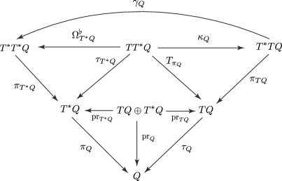
Figure 2.1: A diagram of the canonical diffeomorphisms and bundle projections.

Lagrange-Dirac dynamical systems.

Let us quickly review from Yoshimura, Marsden [2006a, b] the theory of implicit Lagrangian systems or Lagrange-Dirac systems. Let $L:TQ\to\mathbb{R}$ be a Lagrangian, possibly degenerate. The differential $\mathbf{d}L:TQ\rightarrow T^{\ast}(TQ)$ of $L$ is the one-form on $TQ$ locally given by

$$\mathbf{d}L(q,v)=\left(q,v,\frac{\partial L}{\partial q},\frac{\partial L}{\partial v}\right).$$

Using the canonical diffeomorphism $\gamma_{Q}:T^{\ast}(TQ)\rightarrow T^{\ast}(T^{\ast}Q)$, we define the Dirac differential of $L$ by

$$\mathbf{d}_{D}L:=\gamma_{Q}\circ\mathbf{d}L\in\Gamma(T^{\ast}T^{\ast}Q),$$

which is locally given by

$$\mathbf{d}_{D}L(q,v)=\left(q,\frac{\partial L}{\partial v},-\frac{\partial L}{\partial q},v\right).$$

Definition 2.4 (Lagrange-Dirac dynamical systems).

Let $\Delta_{Q}\subset TQ$ be a distribution on $Q$ and consider the induced Dirac structure $D_{\Delta_{Q}}$ on $T^{\ast}Q$. The equations of motion of a Lagrange-Dirac dynamical system (or an implicit Lagrangian system) $(Q,\Delta_{Q},L)$ are given by

$$\left((q(t),p(t),\dot{q}(t),\dot{p}(t)),\mathbf{d}_{D}L(q(t),v(t))\right)\in D_{\Delta_{Q}}(q(t),p(t)).$$ (2.8)

Any curve $(q(t),v(t),p(t))\in TQ\oplus T^{\ast}Q,\,t_{1}\leq t\leq t_{2}$ satisfying (2.8) is called a solution curve of the Lagrange-Dirac dynamical system.

It follows from (2.7) and (2.8) that $(q(t),v(t),p(t))$, $t_{1}\leq t\leq t_{2}$ is a solution curve if and only if it satisfies the implicit Lagrange-d’Alembert equations

$$p=\frac{\partial L}{\partial v},\quad\frac{dq}{dt}=v\in\Delta(q),\quad\frac{dp}{dt}-\frac{\partial L}{\partial q}\in\Delta(q)^{\circ}.$$

Remark 2.5.

Note that the equation $p={\partial L}/{\partial v}$ arises from the equality of the base points $(q,p)$ and $\left(q,{\partial L}/{\partial v}\right)$ in (2.8).

Energy conservation for implicit Lagrangian systems.

Let $(Q,\Delta_{Q},L)$ be a Lagrange-Dirac dynamical system. Define the energy function $E$ on $TQ\oplus T^{\ast}Q$ by

$$E(q,v,p)=\langle p,v\rangle-L(q,v).$$

If $(q(t),v(t),p(t))$ in $TQ\oplus T^{\ast}Q$ is a solution curve of the Lagrange-Dirac system $(Q,\Delta_{Q},L)$, then the energy $E(q(t),v(t),p(t))$ is constant in time. This is shown as follows:

$$\frac{d}{dt}E=\left\langle\dot{p},v\right\rangle+\left\langle p,\dot{v}\right\rangle-\frac{\partial L}{\partial q}\dot{q}-\frac{\partial L}{\partial v}\dot{v}=\left\langle\dot{p}-\frac{\partial L}{\partial q},v\right\rangle,$$

which vanishes since $\dot{q}=v\in\Delta(q)$ and since $\dot{p}-{\partial L}/{\partial q}\in\Delta(q)^{\circ}$.

Hamilton-Dirac dynamical systems.

If the Lagrangian $L$ on $TQ$ is hyperregular, one can define a Hamiltonian $H$ on $T^{\ast}Q$ by Legendre transformation

$$H:=E\circ\mathbb{F}L^{-1},$$

where $E(v_{q})=\left<\mathbb{F}L(v_{q}),v_{q}\right>-L(v_{q})$.

Definition 2.6 (Hamilton-Dirac dynamical system).

Given a Hamiltonian $H:T^{\ast}Q\to\mathbb{R}$ and an induced Dirac structure $D_{\Delta_{Q}}$ on $T^{\ast}Q$, the equations of motion of a Hamilton-Dirac system (also called a implicit Hamiltonian system) $(Q,\Delta_{Q},H)$ are given by

$$((q(t),p(t),\dot{q}(t),\dot{p}(t)),\mathbf{d}H(q(t),p(t)))\in D_{\Delta_{Q}}(q(t),p(t)).$$ (2.9)

Any curve $(q(t),p(t))\in T^{\ast}Q,\,t_{1}\leq t\leq t_{2}$ satisfying (2.9) is called a solution curve of the Hamilton-Dirac dynamical system.

Using (2.7), a curve $(q(t),p(t))$ is a solution curve of the Hamilton-Dirac system $(Q,\Delta_{Q},H)$ if and only if it verifies the Hamilton-d’Alembert equations

$$\dot{q}=\frac{\partial H}{\partial p}\in\Delta,\quad\frac{\partial H}{\partial q}+\dot{p}\in\Delta^{\circ},$$

see Yoshimura, Marsden [2006b].

This is a special instance of an implicit Hamiltonian system on a Poisson manifold, as developed by van der Schaft, Maschke [1995].

A more general geometric setting for constrained implicit Lagrangian and Hamiltonian systems has been developed in Grabowska, Grabowski [2011] via the concept of Dirac algebroids.

2.4 Lie-Dirac reduction

By Lie-Dirac reduction we mean the reduction of a $G$-invariant Dirac structure on $T^{\ast}G$. This process includes the case of the canonical Dirac structure as well as the case of a Dirac structure induced by a nonholonomic constraint. Theses cases have been developed in Yoshimura, Marsden [2007b]. In the present paper we will need two extensions of this theory. First, we will consider the case of Lie-Dirac reduction for an induced Dirac structure, in the presence of an advected parameter. Second we will develop the Lie-Dirac reduction for a more general Dirac structure than the one induced by a nonholonomic constraint.

Invariance and reduction of Dirac structures.

Before going into details on Lie-Dirac reduction, let us just recall the definition of invariant Dirac structures (see, for instance, Dorfman [1993]; Liu, Weinstein, Xu [1998] and Blankenstein, van der Schaft [2001]).

Let $P$ be a manifold and $D$ be a Dirac structure on $P$ with a Lie group $G$ acting on $P$. We denote this action by $\Phi:G\times P\to P$ and the action of a group element $h\in G$ on a point $x\in P$ by $h\cdot x=\Phi(h,x)=\Phi_{h}(x)$ for $h\in G$ and $x\in P$, so that $\Phi_{h}:P\to P$. Then, a Dirac structure $D\subset TP\oplus T^{\ast}P$ is $G$–invariant if

$$((\Phi_{h})_{\ast}X,(\Phi_{h})_{\ast}\alpha)\in D$$ (2.10)

for all $h\in G$ and $(X,\alpha)\in D$.

Suppose that the action $\Phi$ is free and proper and consider its natural lift on the Pontryagin bundle $TP\oplus T^{*}P$. The quotient space $(TP\oplus T^{*}P)/G=(TP)/G\oplus(T^{*}P)/G$ is called the reduced Pontryagin bundle. It is easily checked that the natural lift of the $G$-action to the Pontryagin bundle preserves the symmetric paring (as well as the Courant bracket). Similarly as before, a subbundle $D\subset(TP)/G\oplus(T^{*}P)/G$ is called a Dirac subbundle if for all $x\in P/G$, the vector space $D(x)\subset V\oplus V^{\ast}$, with $V=((TP)/G)_{x}$ is a Dirac structure on $V$. If we suppose that the Dirac structure $D\subset TP\oplus T^{*}P$ is $G$-invariant, then the quotient space $D/G$ is easily verified to be a Dirac subbundle of the reduced Pontryagin bundle. The reduction procedure of Dirac structures $D/G\subset(TP/G)\oplus(T^{\ast}P/G)$ was developed by Yoshimura, Marsden [2007b] for the case $P=T^{\ast}G$ and by Yoshimura, Marsden [2009] for the case $P=T^{\ast}Q$ in the unconstrained case. The reduced Pontryagin bundle $(TP)/G\oplus(T^{*}P)/G$ is an example of a Courant algebroid in the general sense of Liu, Weinstein, Xu [1998], although the algebroid structure was not explicitly utilized in the reduction procedures of Dirac structures.

Induced Dirac structures on $T^{\ast}G$ and trivialized expressions.

As in (2.2), assume that the constraint distribution $\Delta_{G}\subset TG$ on $G$ is left invariant under the group action. We denote, as before, by $\Delta_{T^{\ast}G}$ the lifted distribution on $T^{\ast}G$ and by $D_{\Delta_{G}}$ the induced Dirac structure on $T^{\ast}G$.

Let $\bar{\lambda}:T^{*}G\rightarrow G\times\mathfrak{g}^{\ast}$ be the left trivialization of the cotangent bundle. The trivialized lifted distribution $\Delta_{G\times\mathfrak{g}^{\ast}}$ on $G\times\mathfrak{g}^{\ast}$ is defined by $\Delta_{G\times\mathfrak{g}^{\ast}}:=(T\bar{\pi}_{G})^{-1}(\Delta_{G})$, where $\bar{\pi}_{G}:G\times\mathfrak{g}^{\ast}\to G$ is defined such that $\pi_{G}=\bar{\pi}_{G}\circ\bar{\lambda}$. For each $(g,\mu)\in G\times\mathfrak{g}^{\ast}$, we get

$$\Delta_{G\times\mathfrak{g}^{\ast}}(g,\mu)=\left\{(v_{g},\rho)\in T_{g}G\times\mathfrak{g}^{\ast}\mid v\in\Delta_{G}(g)\right\}=\Delta_{G}(g)\times\{\mu\}\times\mathfrak{g}^{\ast}.$$

We define the trivialized Dirac structure on $G\times\mathfrak{g}^{\ast}$ by

$$\bar{D}_{\Delta_{G}}:=\bar{\lambda}_{\ast}D_{\Delta_{G}}\subset T(G\times\mathfrak{g}^{\ast})\oplus T^{*}(G\times\mathfrak{g}^{\ast}).$$

For each $(g,\mu)\in G\times\mathfrak{g}^{\ast}$, we have

$$\begin{split}\bar{D}_{\Delta_{G}}(g,\mu)&=\{(v_{g},\rho),(\beta_{g},\eta)\in(T_{g}G\times\mathfrak{g}^{\ast})\times(T_{g}^{\ast}G\times\mathfrak{g})\mid(v_{g},\rho)\in\Delta_{G\times\mathfrak{g}^{\ast}}(g,\mu),\\ \text{and}&\;\;\langle\beta_{g},w_{g}\rangle+\langle\sigma,\eta\rangle=\omega(g,\mu)((v_{g},\rho),(w_{g},\sigma)),\;\;\text{for all}\;\;(w_{g},\sigma)\in\Delta_{G\times\mathfrak{g}^{\ast}}(g,\mu)\},\end{split}$$

where $\omega=\bar{\lambda}_{\ast}\Omega$ is the canonical symplectic structure on $G\times\mathfrak{g}^{\ast}$ given, at each point $(g,\mu)\in G\times\mathfrak{g}^{\ast}$, by

$$\omega(g,\mu)((v_{g},\rho),(w_{g},\sigma))=\langle\sigma,g^{-1}v_{g}\rangle-\langle\rho,g^{-1}w_{g}\rangle+\langle\mu,[g^{-1}v_{g},g^{-1}w_{g}]\rangle,$$

where $(w_{g},\sigma)\in T_{(g,\mu)}(G\times\mathfrak{g}^{\ast})\cong T_{g}G\times\mathfrak{g}^{\ast}$.

Invariance and reduction of the induced Dirac structure.

From the $G$-invariance (2.2) of the distribution $\Delta_{G}$, we deduce that it is uniquely determined by its value at $e$, which we denote as

$$\mathfrak{g}^{\Delta}:=\Delta_{G}(e)\subset T_{e}G=\mathfrak{g}.$$

Similarly, the distribution $\Delta_{G\times\mathfrak{g}^{\ast}}\subset T(G\times\mathfrak{g}^{\ast})$ can be completely determined by its values at $(e,\mu)$, for all $\mu\in\mathfrak{g}$, given by

$$\Delta_{G\times\mathfrak{g}^{\ast}}(e,\mu)=\mathfrak{g}^{\Delta}\times\mathfrak{g}^{\ast}\subset T_{(e,\mu)}(G\times\mathfrak{g}^{\ast})\cong\mathfrak{g}\times\mathfrak{g}^{\ast}.$$

Let us denote by $\Lambda_{h}(g,\mu):=(hg,\mu)$ the left $G$-action on $G\times\mathfrak{g}^{\ast}$ induced, via $\bar{\lambda}$, by the cotangent lift of left translation by $G$ on $T^{*}G$. From the invariance of $\Delta_{G}$, it follows that the induced Dirac structure $\bar{D}_{\Delta_{G}}$ on $G\times\mathfrak{g}^{\ast}$ is also $G$–invariant, i.e.

$$((\Lambda_{{h}})_{\ast}X,(\Lambda_{{h}})_{\ast}\alpha)\in\bar{D}_{\Delta_{G}},$$

for all $(X,\alpha)\in\bar{D}_{\Delta_{G}}$ and $h\in G$, as in (2.10). In particular, $\bar{D}_{\Delta_{G}}$ can be uniquely determined by its expression at $(e,\mu)$ as

$$\begin{split}\bar{D}_{\Delta_{G}}(e,\mu)=&\{((\xi,\rho),(\beta,\eta))\in W\oplus W^{\ast}\mid(\xi,\rho)\in\mathfrak{g}^{\Delta}\oplus\mathfrak{g}^{\ast},\\ &\;\text{and}\;\langle\beta,\zeta\rangle+\langle\sigma,\eta\rangle=\omega(e,\mu)((\xi,\rho),(\zeta,\sigma))\;\;\text{for all}\;\;(\zeta,\sigma)\in\mathfrak{g}^{\Delta}\oplus\mathfrak{g}^{\ast}\},\end{split}$$

where $W:=\mathfrak{g}\times\mathfrak{g}^{\ast}$.

Hence, the reduction of the induced Dirac structure $D_{\Delta_{G}}$ can be obtained by taking the quotients by $G$, which is denoted $D_{\Delta_{G}}^{/G}(\mu)$. For each $\mu\in\mathfrak{g}^{\ast}$, we obtain

$$\begin{split}D_{\Delta_{G}}^{/G}(\mu)=&\{((\xi,\rho),(\beta,\eta))\in W\oplus W^{\ast}\mid(\xi,\rho)\in\mathfrak{g}^{\Delta}\oplus\mathfrak{g}^{\ast},\\ &\text{and}\;\;\langle\beta,\zeta\rangle+\langle\sigma,\eta\rangle=\omega^{/G}(\mu)((\xi,\rho),(\zeta,\sigma))\;\;\text{for all}\;\;(\zeta,\sigma)\in\mathfrak{g}^{\Delta}\oplus\mathfrak{g}^{\ast}\},\end{split}$$

where $\omega^{/G}(\mu)$ is the $\mu$-dependent symplectic structure on $W$ given by

$$\omega^{/G}(\mu)((\xi,\rho),(\zeta,\sigma))=\left\langle\sigma,\xi\right\rangle-\left\langle\rho,\zeta\right\rangle+\left\langle\mu,[\xi,\zeta]\right\rangle,$$

where we note that it consists of the canonical two-form as well as the Lie-Poisson structure.

Thus, it follows that for fixed $\mu\in\mathfrak{g}^{\ast}$, the reduced structure $D_{\Delta_{G}}^{/G}(\mu)$ is given by

$$D_{\Delta_{G}}^{/G}(\mu)=\{((\xi,\rho),(\beta,\eta))\in W\oplus W^{\ast}\mid\eta=\xi\in\mathfrak{g}^{\Delta},\;\beta+\rho-\mathrm{ad}_{\xi\,}^{\ast}\mu\in(\mathfrak{g}^{\Delta})^{\circ}\}.$$ (2.11)

As mentioned earlier, $D_{\Delta_{G}}^{/G}$ is automatically a Dirac structure in the reduced Pontryagin bundle $\left(T(T^{*}G)\oplus T^{*}(T^{*}G)\right)/G\cong\mathfrak{g}^{\ast}\times(W\oplus W^{\ast})\rightarrow\mathfrak{g}^{\ast}$. As to the details, see Yoshimura, Marsden [2007b].

2.5 Euler-Poincaré-Dirac reduction

In this section, making use of the Lie-Dirac reduction, we will recall the reduction of a Lagrange-Dirac dynamical system $(G,\Delta_{G},L)$, where we assume that the constraint distribution $\Delta_{G}\subset TG$ is left $G$-invariant. In particular, we will show how the reduced Lagrange-Dirac system can be obtained in an implicit version of the so-called Euler-Poincaré-Suslov equations for nonholonomic mechanics and we also illustrate an example of the Suslov problem of rigid body systems with nonholonomic constraints.

Implicit Lagrangian systems on Lie groups.

Let $G$ be a Lie group, let $D_{\Delta_{G}}$ be the Dirac structure induced from a given distribution $\Delta_{G}$ and let $L$ be a Lagrangian (possibly degenerate) on $TG$. Recall that the equations of motion of a Lagrange-Dirac system $(G,\Delta_{G},L)$ is given by

$$((g,p,\dot{g},\dot{p}),\mathbf{d}_{D}L(g,v))\in D_{\Delta_{G}}(g,p).$$

Recall also that the canonical two-form $\Omega$ on $T^{\ast}G$ is given in coordinates by

$$\Omega\left((g,p,u_{1},\alpha_{1}),(g,p,u_{2},\alpha_{2})\right)=\left\langle\alpha_{2},u_{1}\right\rangle-\left\langle\alpha_{1},u_{2}\right\rangle,$$

and the induced Dirac structure may be expressed, in coordinates, by

$$D_{\Delta_{G}}(g,p)=\left\{\left((g,p,\dot{g},\dot{p}),(g,p,\alpha,w)\right)\mid\dot{g}\in\Delta(g),\;\;w=\dot{g},\;\;\mbox{and}\;\;\alpha+\dot{p}\in\Delta(g)^{\circ}\right\}.$$

Writing $\mathbf{d}_{D}L=(g,p=\partial{L}/\partial{v},-\partial{L}/\partial{g},v)$ and using the local expressions for the canonical symplectic form and the Dirac differential, the equations of motion $((g,p,\dot{g},\dot{p}),\mathbf{d}_{D}L(g,p))\in D_{\Delta_{G}}(g,p)$ read

$$\left\langle-\frac{\partial L}{\partial g},u\right\rangle+\left\langle\alpha,v\right\rangle=\left\langle\alpha,\dot{g}\right\rangle-\left\langle\dot{p},u\right\rangle,$$

for all $u\in\Delta(g)$ and all $\alpha$, where $(u,\alpha)$ are the local representatives of a point in $T_{(g,p)}T^{\ast}G$. Since this holds for all $u\in\Delta(g)$ and all $\alpha$, it follows

$$p=\frac{\partial L}{\partial v},\quad\dot{g}=v\in\Delta(g),\quad\dot{p}-\frac{\partial L}{\partial g}\in\Delta(g)^{\circ},$$ (2.12)

which are the local expressions for the implicit Lagrangian system over $G$.

Left trivialized expressions.

Utilizing the left trivializing diffeomorphism

$$\lambda:TG\to G\times\mathfrak{g},\quad v_{g}\mapsto(g,\eta=g^{-1}v_{g}),$$

we can trivialize $T^{\ast}(TG)$ and $T^{\ast}(T^{\ast}G)$ as $(G\times\mathfrak{g})\times(\mathfrak{g}^{\ast}\oplus\mathfrak{g}^{\ast})$ and $(G\times\mathfrak{g}^{\ast})\times(\mathfrak{g}^{\ast}\oplus\mathfrak{g})$, respectively. Using these trivializations, the map $\mathbf{d}L:TG\rightarrow T^{*}TG$ read

$$\overline{\mathbf{d}L}:G\times\mathfrak{g}\to(G\times\mathfrak{g})\times(\mathfrak{g}^{\ast}\oplus\mathfrak{g}^{\ast}),\quad\overline{\mathbf{d}L}(g,\eta)=\left(g,\eta,g^{-1}\,\frac{\partial{\bar{L}}}{\partial{g}},\,\frac{\partial{\bar{L}}}{\partial{\eta}}\right),$$

where $\bar{L}:=L\circ\lambda^{-1}:G\times\mathfrak{g}\rightarrow\mathbb{R}$. Further, the map $\gamma_{G}:T^{*}TG\rightarrow T^{*}T^{*}G$ is to be

$$\bar{\gamma}_{G}:(G\times\mathfrak{g})\times(\mathfrak{g}^{\ast}\oplus\mathfrak{g}^{\ast})\to(G\times\mathfrak{g}^{\ast})\times(\mathfrak{g}^{\ast}\oplus\mathfrak{g}),\quad\bar{\gamma}_{G}(g,\eta,\nu,\mu)=(g,\mu,-\nu,\eta).$$

Then, the trivialization of the Dirac differential $\mathbf{d}_{D}L:TG\to T^{\ast}T^{\ast}G$ becomes

$$\overline{\mathbf{d}_{D}L}=\bar{\gamma}_{G}\circ\overline{\mathbf{d}L}:G\times\mathfrak{g}\to(G\times\mathfrak{g}^{\ast})\times(\mathfrak{g}^{\ast}\oplus\mathfrak{g}),\quad\overline{\mathbf{d}_{D}L}(g,\eta)=\left(g,\frac{\partial{\bar{L}}}{\partial{\eta}},-g^{-1}\frac{\partial{\bar{L}}}{\partial{g}},\,\eta\right).$$

Note that $\bar{\gamma}_{G}$ is $G$-invariant and induces the map

$$(\bar{\gamma}_{G})^{/G}:\mathfrak{g}\times(\mathfrak{g}^{\ast}\oplus\mathfrak{g}^{\ast})\to\mathfrak{g}^{\ast}\times(\mathfrak{g}^{\ast}\oplus\mathfrak{g}),\quad(\bar{\gamma}_{G})^{/G}(\eta,\nu,\mu)=(\mu,-\nu,\eta).$$

If we assume that $L$ is $G$-invariant, with the associated reduced Lagrangian $\ell:\mathfrak{g}\to\mathbb{R}$, then $\overline{\mathbf{d}L}$ is also $G$-invariant and it induces the quotient map

$$(\overline{\mathbf{d}L})^{/G}:\mathfrak{g}\rightarrow\mathfrak{g}\times(\mathfrak{g}^{\ast}\oplus\mathfrak{g}^{\ast}),\quad(\overline{\mathbf{d}L})^{/G}(\eta)=\left(\eta,0,\frac{\delta{\ell}}{\delta{\eta}}\right).$$

This leads to the following definition.

Definition 2.7.

The reduced Dirac differential of $\ell:\mathfrak{g}\rightarrow\mathbb{R}$ is

$$\mathbf{d}^{/G}_{D}\ell:=(\overline{\mathbf{d}_{D}L})^{/G}=(\bar{\gamma}_{G})^{/G}\circ(\overline{\mathbf{d}L})^{/G}:\mathfrak{g}\rightarrow\mathfrak{g}^{\ast}\times(\mathfrak{g}^{\ast}\oplus\mathfrak{g}),$$

whose expression is

$$\mathbf{d}^{/G}_{D}\ell(\eta)=\left(\frac{\delta{\ell}}{\delta{\eta}},0,\eta\right).$$ (2.13)

Remark 2.8.

Note that the usual differential of the reduced Lagrangian $\ell:\mathfrak{g}\to\mathbb{R}$ is the map

$$\mathbf{d}\ell:\mathfrak{g}\to\mathfrak{g}\times\mathfrak{g}^{\ast},\quad\mathbf{d}\ell(\eta)=\left(\eta,\frac{\delta l}{\delta\eta}\right).$$

It has therefore a different target space (and, of course, a different expression) from the reduced Dirac differential $\mathbf{d}^{/G}_{D}\ell:\mathfrak{g}\rightarrow\mathfrak{g}^{\ast}\times(\mathfrak{g}^{\ast}\oplus\mathfrak{g})$.

Euler-Poincaré-Dirac reduction.

Let us recall the definition of reduction of an implicit Lagrangian system associated with the induced Dirac structure on $T^{\ast}G$.

Definition 2.9 (Reduced Lagrange-Dirac dynamical system).

Let $(G,\Delta_{G},L)$ be a Lagrange-Dirac dynamical system. The equations of motion for the reduced Lagrange-Dirac dynamical system are given by

$$\left((\mu(t),\xi(t),\dot{\mu}(t)),\mathbf{d}^{/G}_{D}\ell(\eta(t))\right)\in D_{\Delta_{G}}^{/G}(\mu(t)).$$ (2.14)

In the above, $(\eta(t),\mu(t))\in\mathfrak{g}\oplus\mathfrak{g}^{\ast}$ is the reduced curve associated to $(g(t),v(t),p(t))\in TG\oplus T^{\ast}G$ and $(\mu(t),\xi(t),\dot{\mu}(t))\in\mathfrak{g}^{\ast}\times V$ is the reduced curve associated to $(g(t),p(t),\dot{g}(t),\dot{p}(t))$. Note also that (2.14) induces the equality of the base points, i.e. $\mu(t)=\mathbb{F}{\ell}(\eta(t))$.

Definition 2.10.

Any curve $(\xi(t),\mu(t))$ in $\mathfrak{g}\oplus\mathfrak{g}^{\ast}$ together with $\mu(t)=\mathbb{F}{\ell}(\eta(t))$ for $\eta(t)\in\mathfrak{g}$ satisfying (2.14) is called a solution curve of the reduced Lagrange-Dirac dynamical system.

It follows from equations (2.11), (2.13) and (2.14) that $(\xi(t),\mu(t))$ is a solution curve of the reduced Lagrange-Dirac dynamical system if and only if it satisfies

$$\mu=\frac{\delta{\ell}}{\delta\eta},\quad\xi=\eta\in\mathfrak{g}^{\Delta},\quad\dot{\mu}-\mathrm{ad}_{\xi}^{\ast}\mu\in(\mathfrak{g}^{\Delta})^{\circ},$$ (2.15)

where $(\mathfrak{g}^{\Delta})^{\circ}\subset\mathfrak{g}^{\ast}$ is the annihilator of the constraint subspace $\mathfrak{g}^{\Delta}$.

The set of equations of motion in equation (2.15) is the local expression for the reduction of the implicit Lagrange-d’Alembert equations given in equation (2.12), which is an implicit analog of Euler-Poincaré-Suslov equations (see Bloch [2003]). The set of equations of motion in (2.15) is called implicit Euler-Poincaré-Suslov equations for nonholonomic mechanics (see Yoshimura, Marsden [2007b]).

Energy conservation of the reduced Lagrange-Dirac dynamical system.

Let us denote by $(G,\Delta_{G},L)$ a Lagrange-Dirac dynamical system. Recall that the generalized energy $E$ is defined by $E(g,v,p):=\left(p,v\right>-L(g,v)$, which is $G$-invariant under the action of $G$ since $L$ is $G$–invariant and one easily checks that the momentum function $\langle p(t),v(t)\rangle$ is also $G$-invariant. Hence one can define the reduced energy $e$ on $\mathfrak{g}\oplus\mathfrak{g}^{\ast}$ by, for $(\eta,\mu)\in\mathfrak{g}\oplus\mathfrak{g}^{\ast}$,

$$e(\eta,\mu)=\left\langle\mu,\eta\right\rangle-\ell(\eta),$$

where $\ell=L|\mathfrak{g}$ is the reduced Lagrangian on $\mathfrak{g}$ and $\left\langle\mu,\eta\right\rangle$ is the reduced momentum function on $\mathfrak{g}\oplus\mathfrak{g}^{\ast}$. We denote by $\mathfrak{g}^{\Delta}\subset\mathfrak{g}$ the reduction of $\Delta_{G}\subset TG$. Let $(\eta(t),\mu(t))$ be a solution curve of the reduced Lagrange-Dirac dynamical system. Then conservation of energy holds along the solution curve $(\eta(t),\mu(t))$; that is, the (reduced) energy $e(\eta(t),\mu(t))$ is constant in time, because it follows, by noting that $\mu(t)=(\delta\ell/\delta\eta)(t)$,

$$\frac{d}{dt}e(\eta,\mu)=\left\langle\dot{\mu},\eta\right\rangle+\left\langle\mu,\dot{\eta}\right\rangle-\left\langle\frac{\delta\ell}{\delta\eta},\dot{\eta}\right\rangle=\left\langle{\mu}-\frac{\delta\ell}{\delta\eta},\dot{\eta}\right\rangle+\left\langle\mathrm{ad}^{\ast}_{\xi}\mu,\eta\right\rangle=\left\langle\mathrm{ad}^{\ast}_{\xi}\mu,\xi\right\rangle,$$

which vanishes since $\eta=\xi\in\mathfrak{g}^{\Delta}$ and since $\dot{\mu}-\mathrm{ad}^{\ast}_{\xi}\mu\in(\mathfrak{g}^{\Delta})^{\circ}$.

2.6 Lie-Poisson-Dirac reduction

For the case in which a given Lagrangian is regular, or when a Hamiltonian is given, we can develop a Hamiltonian analogue of Euler-Poincaré-Dirac reduction. This section gives a reduction procedure for a Hamilton-Dirac dynamical system $(G,\Delta_{G},H)$ associated with an induced Dirac structure on $D_{\Delta_{G}}$, which we shall call Lie-Poisson-Dirac reduction. It is also shown that this reduction procedure may be also useful in the analysis of the Suslov problem in nonholonomic mechanics.

Implicit Hamiltonian systems over Lie groups.

Let $G$ be a Lie group, $D_{\Delta_{G}}$ be an induced Dirac structure from a given left invariant distribution $\Delta_{G}$, and $H$ be a $G$-invariant Hamiltonian on $T^{\ast}G$. Recall that equations of motion of a Hamilton-Dirac dynamical system $(G,\Delta_{G},H)$ are given by

$$\left((g(t),p(t),\dot{g}(t),\dot{p}(t)),\mathbf{d}H(g(t),p(t))\right)\in D_{\Delta_{G}}(g(t),p(t)),$$

which read, by using the local expressions for the canonical symplectic form and the differential of $H$, namely, $\mathbf{d}H=(g,p,\partial{H}/\partial{g},\partial{H}/\partial{p})$,

$$\left\langle\frac{\partial H}{\partial g},u\right\rangle+\left\langle\alpha,\frac{\partial H}{\partial p}\right\rangle=\left\langle\alpha,\dot{g}\right\rangle-\left\langle\dot{p},u\right\rangle,$$

for all $u\in\Delta(g)$ and all $\alpha$, where $(u,\alpha)$ are the local representatives of a point in $T_{(g,p)}T^{\ast}G$. It follows that the local expressions for the implicit Hamiltonian system is

$$\dot{g}=\frac{\partial H}{\partial p}\in\Delta(g),\quad\dot{p}+\frac{\partial H}{\partial g}\in\Delta(g)^{\circ}.$$

Lie-Poisson-Dirac reduction.

Let us develop the reduction procedure for the Hamilton-Dirac dynamical system over a Lie group, which we shall call Lie-Poisson-Dirac Reduction. The induced Hamiltonian $\bar{H}$ on $G\times\mathfrak{g}^{\ast}$ is $G$–invariant, and it reads

$$\bar{H}(g,\mu)=h(\mu),$$

where $h:\mathfrak{g}^{\ast}\to\mathbb{R}$ is the reduced Hamiltonian as a trivialized expression of $h=H^{/G}=H|{\mathfrak{g}^{\ast}}$.

Trivialized expressions.

Employing the trivializing diffeomorphism

$$\bar{\lambda}:T^{\ast}G\to G\times\mathfrak{g}^{\ast},\quad\alpha_{g}\mapsto(g,\mu=T_{e}^{\ast}L_{g}(\alpha_{g})),$$

and defining the trivialization $\bar{H}=H\circ\bar{\lambda}^{-1}$, we note that the differential $\mathbf{d}H:T^{*}G\rightarrow T^{*}T^{*}G$ can be trivialized as the map

$$\overline{\mathbf{d}H}:G\times\mathfrak{g}^{\ast}\to(G\times\mathfrak{g}^{\ast})\times(\mathfrak{g}^{\ast}\oplus\mathfrak{g}),\quad\overline{\mathbf{d}H}(g,\mu)=\left(g,\mu,g^{-1}\,\frac{\partial{\bar{H}}}{\partial{g}},\frac{\partial{\bar{H}}}{\partial{\mu}}\right),$$

Suppose that $H$ is $G$-invariant, with reduced Hamiltonian $h:\mathfrak{g}^{\ast}\rightarrow\mathbb{R}$. Then the map $\overline{\mathbf{d}H}$ induces a map $(\mathbf{d}\bar{H})^{/G}$ on the quotient. We define the reduction of the differential operator for $h$ as the map

$$\mathbf{d}^{/G}h:=(\overline{\mathbf{d}H})^{/G}:\mathfrak{g}^{\ast}\rightarrow\mathfrak{g}^{\ast}\times(\mathfrak{g}^{\ast}\oplus\mathfrak{g}),\quad\mathbf{d}^{/G}h(\mu)=\left(\mu,0,\frac{\delta{h}}{\delta{\mu}}\right).$$ (2.16)

Definition 2.11 (Reduced Hamilton-Dirac dynamical system).

Let $(G,\Delta_{G},H)$ be a Hamilton-Dirac dynamical system. The equations of motion for the reduced Hamilton-Dirac dynamical system may be given by

$$((\mu(t),\xi(t),\dot{\mu}(t)),\mathbf{d}^{/G}h(\mu(t)))\in D_{\Delta_{G}}^{/G}(\mu(t)).$$ (2.17)

Definition 2.12.

A curve $(\xi(t),\mu(t))$ in $\mathfrak{g}\oplus\mathfrak{g}^{\ast}$ is a solution curve of the reduced Hamilton-Dirac dynamical system if and only if it satisfies (2.17).

It follows from equations (2.11), (2.16) and (2.17) that $(\xi(t),\mu(t))\in\mathfrak{g}\oplus\mathfrak{g}^{\ast}$ is a solution curve of the reduced Hamilton-Dirac dynamical system if and only if it satisfies

$$\dot{\mu}-\mathrm{ad}_{\xi}^{\ast}\mu\in(\mathfrak{g}^{\Delta})^{\circ},\quad\xi=\frac{\delta{h}}{\delta\mu}\in\mathfrak{g}^{\Delta},$$ (2.18)

where $(\mathfrak{g}^{\Delta})^{\circ}\subset\mathfrak{g}^{\ast}$ is the annihilator of the constraint subspace $\mathfrak{g}^{\Delta}$. The set of equations in equation (2.18) is called implicit Lie-Poisson-Suslov equations for nonholonomic mechanics (see Yoshimura, Marsden [2007b]).

3 Semidirect product theory

The theory of Lie-Poisson reduction for semidirect products has been systematically developed in Marsden, Ratiu, Weinstein [1984]; see also Marsden et al [1983], and applied to several examples in mechanics such as the heavy top, compressible fluids, and magnetohydrodynamics. One of the main features of this approach is that it allows one to obtain the noncanonical Hamiltonian (or Poisson) structure of the dynamical system by reduction of the canonical symplectic structure on the cotangent bundle of the configuration Lie group. Such a reduction approach to noncanonical Poisson structures has been developed by Marsden, Weinstein [1983] for incompressible perfect fluid motion, based on the earlier work of Arnol’d [1966].

The Lagrangian side of the semidirect Lie-Poisson reduction has been developed in Holm, Marsden, Ratiu [1998] in connection with several examples in fluid dynamics. We will refer to this reduction theory as Euler-Poincaré reduction with advected parameters (which is not the same as Euler-Poincaré reduction for semidirect products, see Remark 3.4 later).

Semidirect products.

Let $G$ be a Lie group acting by left representation on a vector space $V$. We will denote by $v\mapsto\rho_{g}(v)$ or simply by $v\mapsto gv$ the left representation of $g\in G$ on $v\in V$. The semidirect product $S=G\,\circledS\,V$ is the Cartesian product $S=G\times V$ whose group multiplication is given by

$$(g_{1},v_{1})(g_{2},v_{2})=(g_{1}g_{2},v_{1}+g_{1}v_{2})=(g_{1}g_{2},v_{1}+\rho_{g_{1}}v_{2}).$$

The identity element is $(e,0)$, where $e$ is the identity in $G$, and the inverse of an element $(g,v)$ is given by $(g^{-1},-g^{-1}v)$. Let $\mathfrak{g}$ be the Lie algebra of $G$. The induced Lie algebra action of $\mathfrak{g}$ on $V$ is given, for $\xi\in\mathfrak{g}$ and $v\in V$, by

$$\xi v:=\rho^{\prime}(\xi)v:=\frac{d}{dt}\biggr{|}_{t=0}\rho_{\mathrm{exp}(\xi t)}v\in V,$$

where $\rho^{\prime}:\mathfrak{g}\to\mathrm{End}(V)$ is the induced Lie algebra representation. In this paper, we will employ the concatenation notation $\xi v$ most commonly.

The Lie algebra $\mathfrak{s}$ is the semidirect product $\mathfrak{s}:=\mathfrak{g}\,\circledS\,V$ of $\mathfrak{g}$ with $V$ endowed with the Lie bracket

$$\begin{split}[(\xi_{1},v_{1}),(\xi_{2},v_{2})]&=([\xi_{1},\xi_{2}],\rho^{\prime}(\xi_{1})v_{2}-\rho^{\prime}(\xi_{2})v_{1})\\ &=([\xi_{1},\xi_{2}],{\xi_{1}}v_{2}-{\xi_{2}}v_{1})=\mathrm{ad}_{(\xi_{1},v_{1})}(\xi_{2},v_{2}),\end{split}$$

where $\xi_{1},\xi_{2}\in\mathfrak{g}$ and $v_{1},v_{2}\in V$.

The adjoint action of $(g,v)\in S$ on $(\xi,u)\in\mathfrak{s}$ is given by

$$\mathrm{Ad}_{(g,v)}(\xi,u)=\left(\mathrm{Ad}_{g}\xi,\rho_{g}u-\rho^{\prime}(\mathrm{Ad}_{g}\xi)u\right),$$

and the coadjoint action of $(g,v)\in S$ on $(\mu,a)\in\mathfrak{s}^{\ast}$ reads

$$\mathrm{Ad}^{\ast}_{(g,v)^{-1}}(\mu,a)=\left(\mathrm{Ad}^{\ast}_{g^{-1}}\mu+(\rho^{\prime}_{v})^{\ast}\rho^{*}_{g^{-1}}a,\rho^{*}_{g^{-1}}a\right).$$

In the above, $\rho_{v}^{\prime}:\mathfrak{g}\to V$ denotes the linear map defined by $\rho_{v}^{\prime}(\xi):=\rho^{\prime}(\xi)v$, the map $(\rho_{v}^{\prime})^{\ast}:V^{\ast}\to\mathfrak{g}^{\ast}$ denotes its dual map, defined by

$$\left<(\rho^{\prime}_{v})^{\ast}(a),\xi\right>=\left<a,\rho^{\prime}_{v}(\xi)\right>=\left<a,\xi v\right>,\;\;\text{for}\;\;\xi\in\mathfrak{g},\;\;v\in V,\;\;a\in V^{\ast},$$

and $\rho^{*}_{g^{-1}}:V^{\ast}\rightarrow V^{\ast}$ is the dual map to the inverse representation $\rho_{g^{-1}}$. We will denote it simply by concatenation as $ga:=\rho^{\ast}_{g^{-1}}a$.

Diamond operator.

Following Holm, Marsden, Ratiu [1998], we will use the diamond notation $\diamond:V\times V^{\ast}\to\mathfrak{g}^{\ast}$, defined by $(v,a)\mapsto v\diamond a:=(\rho^{\prime}_{v})^{\ast}(a)$. We thus have

$$\left<v\diamond a,\xi\right>=\left<a,\xi v\right>=-\left<\xi a,v\right>,\;\;\text{for}\;\;\xi\in\mathfrak{g},\;\;v\in V,\;\;a\in V^{\ast},$$

where

$$\xi a:=\frac{d}{dt}\biggr{|}_{t=0}\rho_{\mathrm{exp}(-t\xi)}^{\ast}a=\frac{d}{dt}\biggr{|}_{t=0}\operatorname{exp}(t\xi)a\in V^{\ast}.$$

Right actions.

When the Lie group acts on the vector space $V$ by a right representation $v\mapsto\rho_{g}v=vg$, there are some changes in the formulas. The group multiplication of $S=G\,\circledS\,V$ is given by

$$(g_{1},v_{1})(g_{2},v_{2})=(g_{1}g_{2},v_{2}+\rho_{g_{2}}v_{1})=(g_{1}g_{2},v_{2}+v_{1}g_{2})$$

and the Lie bracket on $\mathfrak{s}=\mathfrak{g}\,\circledS\,V$ reads

$$\begin{split}\mathrm{ad}_{(\xi_{1},v_{1})}(\xi_{2},v_{2})=[(\xi_{1},v_{1}),(\xi_{2},v_{2})]=([\xi_{1},\xi_{2}],v_{1}\xi_{2}-v_{2}\xi_{1}),\end{split}$$

where $v\mapsto v\xi$ denotes the induced Lie algebra representation on $V$. The adjoint action of $(g,v)\in S$ on $(\xi,u)\in\mathfrak{s}$ is given by

$$\operatorname{Ad}_{(g,v)}(\xi,u)=(\operatorname{Ad}_{g}\xi,(u+v\xi)g^{-1})$$

while the coadjoint action of $(g,v)\in S$ on $(\mu,a)\in\mathfrak{s}^{\ast}$ is

$$\operatorname{Ad}^{\ast}_{(g,v)^{-1}}(\mu,a)=(\operatorname{Ad}^{\ast}_{g^{-1}}\mu+(vg^{-1})\diamond(ag^{-1}),ag^{-1}),$$

where $a\mapsto ag$ denotes the induced right representation of $G$ on $V^{\ast}$. As before, we have used the diamond notation

$$\left<v\diamond a,\xi\right>=\left<a,v\xi\right>=-\left<a\xi,v\right>,\;\;\text{for}\;\;\xi\in\mathfrak{g},\;\;v\in V,\;\;a\in V^{\ast}.$$

Note that, following our conventions, the adjoint and coadjoint actions are left representations.

3.1 Euler-Poincaré reduction with advected parameters

In this section we recall from Holm, Marsden, Ratiu [1998] the theory of Euler-Poincaré reduction with advected parameters. We use the same notation as above concerning the various Lie group and Lie algebra actions arising in the formulas.

• Assume that we have a function $L:TG\times V^{\ast}\rightarrow\mathbb{R}$ which is left $G$-invariant under the action $(v_{h},a)\mapsto(gv_{h},ga)$, where $g,h\in G$, $v_{h}\in TG$, and $a\in V^{\ast}$.

• In particular, given $a_{0}\in V^{\ast}$, we define the Lagrangian $L_{a_{0}}:TG\rightarrow\mathbb{R}$ by $L_{a_{0}}(v_{g}):=L(v_{g},a_{0})$. Then $L_{a_{0}}$ is left invariant under the lift to $TG$ of the left action of $G_{a_{0}}$ on $G$, where $G_{a_{0}}:=\{g\in G\mid ga_{0}=a_{0}\}$ is the isotropy group of $a_{0}$ with respect to the linear action of $G$ on $V^{\ast}$.

• Define the reduced Lagrangian $\ell:\mathfrak{g}\times V^{\ast}\rightarrow\mathbb{R}$ by $\ell:=L|_{\mathfrak{g}\times V^{\ast}}$. Left $G$-invariance of $L$ yields the formula

  $$\ell(g^{-1}v_{g},g^{-1}a_{0})=L(v_{g},a_{0}),$$

  for all $g\in G$, $v_{g}\in T_{g}G$, and $a_{0}\in V^{\ast}$.

• For a curve $g(t)\in G$ with $g(0)=e$, let $\xi(t):=g(t)^{-1}\dot{g}(t)\in\mathfrak{g}$ and define the curve $a(t)\in V^{\ast}$ as the unique solution of the following linear differential equation with time dependent coefficients

  $$\dot{a}+\xi a=0,$$ (3.1)

  with initial condition $a_{0}$. The solution of (3.1) can then be written as

  $$a(t)=g(t)^{-1}a_{0}.$$

Theorem 3.1.

With the preceding notation, the following are equivalent:

• With $a_{0}\in V^{\ast}$ held fixed, Hamilton’s variational principle

  $$\delta\int_{t_{0}}^{t_{1}}L_{a_{0}}(g,\dot{g})\mbox{d}t=0,$$

  holds, for variations $\delta g(t)$ of $g(t)$ vanishing at the endpoints.

• The curve $g(t)$ satisfies the Euler-Lagrange equations for $L_{a_{0}}$ on $G$.

• The constrained variational principle

  $$\delta\int_{t_{0}}^{t_{1}}\ell(\xi,a)\mbox{d}t=0,$$

  holds on $\mathfrak{g}\times V^{\ast}$, upon using variations of the form

  $$\delta\xi=\frac{\partial\eta}{\partial t}+[\xi,\eta],\quad\delta a=-\eta a,$$

  where $\eta(t)\in\mathfrak{g}$ vanishes at the endpoints.

• The Euler-Poincaré equations with advected parameter hold on $\mathfrak{g}\times V^{\ast}$:

  $$\frac{\partial}{\partial t}\frac{\delta\ell}{\delta\xi}=\operatorname{ad}^{\ast}_{\xi}\frac{\delta\ell}{\delta\xi}+\frac{\delta\ell}{\delta a}\diamond a.$$ (3.2)

We refer to Holm, Marsden, Ratiu [1998] for the proof and several applications. Note that the $G$-invariant function $L:TG\times V^{\ast}\rightarrow\mathbb{R}$ is not the Lagrangian of system. The Lagrangian $L_{a_{0}}$ is obtained by fixing a value $a_{0}\in V^{\ast}$, i.e., $L_{a_{0}}(v_{g}):=L(v_{g},a_{0})$ and is only $G_{a_{0}}$-invariant.

3.2 Lie-Poisson reduction on semidirect products

We now recall the theory of Lie-Poisson reduction for semidirect product, following Marsden, Ratiu, Weinstein [1984]. The setup is given as follows:

• Assume that we have a function $H:T^{\ast}G\times V^{\ast}\rightarrow\mathbb{R}$ which is left invariant under the action $(\alpha_{h},a)\mapsto(g\alpha_{h},ga)$, for all $g,h\in G$, $\alpha_{h}\in T^{\ast}G$, and $a\in V^{\ast}$.

• In particular, given $a_{0}\in V^{\ast}$, we define the Hamiltonian $H_{a_{0}}:T^{\ast}G\rightarrow\mathbb{R}$ by

  $$H_{a_{0}}(\alpha_{g}):=H(\alpha_{g},a_{0}).$$

  Then $H_{a_{0}}$ is left invariant under the cotangent lift to $T^{\ast}G$ of the left action of $G_{a_{0}}$ on $G$.

• Define the reduced Hamiltonian $h:\mathfrak{g}^{\ast}\times V^{\ast}\rightarrow\mathbb{R}$ by $h:=H|_{\mathfrak{g}^{\ast}\times V^{\ast}}$. Left $G$-invariance of $H$ yields the formula

  $$h(g^{-1}\alpha_{g},g^{-1}a_{0})=H(\alpha_{g},a_{0}),$$

  for all $g\in G$, $\alpha_{g}\in T_{g}^{\ast}G$, and $a_{0}\in V^{\ast}$.

Theorem 3.2.

For the curves $\alpha(t)\in T^{\ast}_{g(t)}G$ and $\mu(t):=T^{\ast}L_{g(t)}(\alpha(t))\in\mathfrak{g}^{\ast}$, the following are equivalent:

• The curve $\alpha(t)$ satisfies Hamilton’s equations for $H_{a_{0}}$ on $T^{\ast}G$.

• The Lie-Poisson equation holds on $\mathfrak{s}^{\ast}$:

  $$\frac{\partial}{\partial t}(\mu,a)=\operatorname{ad}^{\ast}_{\left(\frac{\delta h}{\delta\mu},\frac{\delta h}{\delta a}\right)}(\mu,a)=\left(\operatorname{ad}^{\ast}_{\frac{\delta h}{\delta\mu}}\mu-\frac{\delta h}{\delta a}\diamond a,-\frac{\delta h}{\delta\mu}a\right),\quad a(0)=a_{0},$$

  where $\mathfrak{s}$ is the semidirect product Lie algebra $\mathfrak{s}=\mathfrak{g}\,\circledS\,V$. The associated Poisson bracket is the Lie-Poisson bracket on the semidirect product Lie algebra $\mathfrak{s}^{\ast}$, that is,

  $$\{f,g\}(\mu,a)=-\left\langle\mu,\left[\frac{\delta f}{\delta\mu},\frac{\delta g}{\delta\mu}\right]\right\rangle-\left\langle a,\frac{\delta f}{\delta\mu}\frac{\delta g}{\delta a}-\frac{\delta g}{\delta\mu}\frac{\delta f}{\delta a}\right\rangle.$$

Like on the Lagrangian side, the evolution of the advected parameter is given by $a(t)=g(t)^{-1}a_{0}$.

Legendre transform.

The link with Euler-Poincaré reduction for advected parameters recalled in §3.1 is the following. Let $L_{a_{0}}:TG\rightarrow\mathbb{R}$ be a given Lagrangian coming from a $G$-invariant function $L:TG\times V^{\ast}\rightarrow\mathbb{R}$, suppose that the Legendre transformation $\mathbb{F}L_{a_{0}}$ is invertible and form the corresponding Hamiltonian $H_{a_{0}}=E_{a_{0}}\circ\mathbb{F}L_{a_{0}}^{-1}$, where $E_{a_{0}}$ is the energy of $L_{a_{0}}$. Then the function $H:T^{\ast}G\times V^{\ast}\rightarrow\mathbb{R}$ so defined is $G$-invariant and one can apply Theorem 3.2. At the reduced level, the Hamiltonian $h:\mathfrak{g}^{\ast}\times V^{\ast}\rightarrow\mathbb{R}$ is given in terms of $\ell$ by

$$h(\mu,a):=\langle\mu,\xi\rangle-\ell(\xi,a),\quad\mu=\frac{\delta\ell}{\delta\xi}.$$

Since

$$\frac{\delta h}{\delta\mu}=\xi\quad\text{and}\quad\frac{\delta h}{\delta a}=-\frac{\delta\ell}{\delta a},$$

we see that the Lie-Poisson equations for $h$ on $\mathfrak{s}^{\ast}$ are equivalent to the Euler-Poincaré equations with advected quantities (3.2) for $\ell$ together with the advection equation $\dot{a}+a\xi=0$.

Remark 3.3 (Links with reduction by stages).

It is surprising, at first glance, that at the reduced level, on the Hamiltonian side, we recover the ordinary Lie-Poisson equations for the semidirect product $S=G\,\circledS\,V$, whereas we started with a $G$-invariant Hamiltonian $H:T^{\ast}G\times V^{\ast}\rightarrow\mathbb{R}$ and not a $S$-invariant Hamiltonian on $T^{\ast}S$. This can be easily justified by the process of Poisson reduction by stages, Marsden et al [2007]. Indeed, the $G$-action on $T^{\ast}G\times V^{\ast}$ can be seen as the action induced by the cotangent lift of left translation on $S$, given by

$$T^{\ast}L_{{(g,v)}^{-1}}(\alpha_{h},(u,a)):=\left(g\alpha_{h},(v+gu,ga)\right).$$

Thus, we can think of the Hamiltonian $H:T^{\ast}G\times V^{\ast}\to\mathbb{R}$ as being the first stage Poisson reduction of a $S$-invariant Hamiltonian $\bar{H}:T^{\ast}S\to\mathbb{R}$ by the normal subgroup $\{e\}\times V\subset S$, since $(T^{\ast}S)/(\{e\}\times V)\cong T^{\ast}G\times V^{\ast}$. Then the second stage of the Poisson reduction applied to $H:T^{\ast}G\times V^{\ast}\rightarrow\mathbb{R}$ yields the reduced Hamiltonian $h$ and the reduced Hamilton equations of motion on $\mathfrak{g}^{\ast}\times V^{\ast}$. By the Poisson reduction by stages theorem, we know that the two-stages reduction coincides with the one step reduction of $\bar{H}$ by $S$ and, therefore, the reduced equations of motion on $\mathfrak{g}^{\ast}\times V^{\ast}$ must recover the Lie-Poisson equations on the semidirect product $\mathfrak{s}$.

Note that the Hamiltonian $H_{a_{0}}$ does not appear in the process of Poisson reduction by stages. In order to obtain it naturally from a reduction approach, it is necessary to use symplectic reduction by stages. Consider the semidirect product Lie group $S=G\,\circledS\,V$ acting by right translation on its cotangent bundle $T^{\ast}S$. An equivariant momentum map relative to the canonical symplectic form is given by

$$\mathbf{J}_{L}(\alpha_{f},(u,a))=T^{\ast}R_{(f,u)}(\alpha_{f},(u,a))=(T^{\ast}_{e}R_{f}(\alpha_{f})+u\diamond a,a).$$

Since $V$ is a closed normal subgroup of $S$, it also acts on $T^{\ast}S$ and has a momentum map $\mathbf{J}_{V}:T^{\ast}S\to V^{\ast}$ given by

$$\mathbf{J}_{V}(\alpha_{f},(u,a))=a.$$

Reducing $T^{\ast}S$ by $V$ at the value $a_{0}$ we get the first stage reduced space $(T^{\ast}S)_{a_{0}}=\mathbf{J}_{V}^{-1}(a_{0})/V$. One observes that this space is symplectically diffeomorphic to the canonical symplectic manifold $(T^{\ast}G,\Omega)$, and that the $S$-invariant Hamiltonian $\bar{H}$ on $T^{\ast}S$ induces exactly the Hamiltonian $H_{a_{0}}$ on $T^{\ast}G\simeq(T^{\ast}S)_{a_{0}}$, as desired. For completeness, we now comment on the second stage symplectic reduction. The isotropy subgroup $G_{a_{0}}$, consisting of elements of $G$ that leave the point $a_{0}$ fixed, acts freely and properly on the first stage symplectic reduced space $(T^{\ast}S)_{a_{0}}$ and admits an equivariant momentum map $\mathbf{J}_{a_{0}}:(T^{\ast}S)_{a_{0}}\to\mathfrak{g}^{\ast}_{a_{0}}$ induced from $\mathbf{J}_{L}$, where $\mathfrak{g}_{a_{0}}$ is the Lie algebra of $G_{a_{0}}$. Reducing $(T^{\ast}S)_{a_{0}}$ at the point $\mu_{a_{0}}:=\mu|\mathfrak{g}_{a_{0}}$, we get the second symplectic reduced space $\left((T^{\ast}S)_{a_{0}}\right)_{\mu_{a_{0}}}=\mathbf{J}_{a}^{-1}(\mu_{a_{0}})/(G_{a_{0}})_{\mu_{a_{0}}}$. From the Reduction by Stages Theorem (Marsden et al [2007]), the second symplectic reduced space $\left((T^{\ast}S)_{a_{0}}\right)_{\mu_{a_{0}}}$ is symplectically diffeomorphic to the symplectic reduced space $(T^{\ast}S)_{(\mu,a_{0})}=\mathbf{J}_{R}^{-1}(\mu,a)/G_{(\mu,a_{0})}$ obtained by symplectic reduction by $S$ at the point $(\mu,a_{0})\in\mathfrak{s}^{\ast}$. The latter is symplectically diffeomorphic to the coadjoint orbit $\left(\mathcal{O}_{(\mu,a_{0})},\omega_{(\mu,a_{0})}\right)$ of $S$ endowed with its orbit symplectic form.

Remark 3.4 (Cautionary remark).

It is important to mention here that the Hamiltonian reduction mentioned above is literally an ordinary Lie-Poisson reduction in the special case when the Lie group is a semidirect product. This is not the case for the Lagrangian side, since it does not coincide with the Euler-Poincaré reduction in the special case when the Lie group is a semidirect product. This is why we prefer to call it Euler-Poincaré reduction with advected parameters. This comment is important for the present paper for two reasons. First, we will see that a crucial example of nonholonomic system arises when the Lie group itself is a semidirect product in addition to have advected quantities. So there are two semidirect products arising in this example and, on the Lagrangian side, they have completely different roles; second, we will see that the Dirac reduction processes involved in the Lagrangian and Hamiltonian side are completely different.

4 Variational framework

The goal of this section is to derive the implicit Euler-Poincaré-Suslov equations with advected parameters together with the associated variational structures. We first consider the unconstrained case via the Hamilton-Pontryagin principle, and then explore the nonholonomic case given by a parameter dependent constraint $\Delta_{G}^{a_{0}}\subset TG$, by using the Lagrange-d’Alembert-Pontryagin principle. Second we study the case of a nonholonomic system in which a configuration Lie group is a semidirect product and with special classes of constraints arising in several examples. In particular, it is shown that the results of Schneider [2002] can be incorporated into the classes of nonholonomic constraints. Finally, we also explore the Hamiltonian side to develop the corresponding implicit Lie-Poisson-Suslov equations with advected parameters, which will be shown to be different from the implicit Lie-Poisson-Suslov equations on semidirect products. We also mention how the theory can be extended to the case in which the parameters are acted on by more general actions, such as affine actions.

4.1 The unconstrained case

Let us consider the Hamilton-Pontryagin principle and its associated reduced version for the case of a parameter dependent Lagrangian $L_{a_{0}}(g,\dot{g})=L(g,\dot{g},a_{0}):TG\times V^{\ast}\to\mathbb{R}$. Using the same notations and assumptions made in the beginning of §3.1, we state the following theorem.

Theorem 4.1.

With the above notations, the following statements are equivalent.

• With $a_{0}$ fixed, the Hamilton-Pontryagin principle

  $$\delta\int_{t_{1}}^{t_{2}}\left\{L_{a_{0}}(g(t),v(t))+\left\langle p(t),\dot{g}(t)-v(t)\right\rangle\right\}\,dt=0$$ (4.1)

  holds for variations $(\delta{g}(t),\delta{v}(t),\delta{p}(t))$ of $(g(t),v(t),p(t))$ in $TG\oplus T^{\ast}G$ such that $\delta g$ vanishes at the endpoints.

• The curve $g(t),\;t\in[t_{1},t_{2}]$ satisfies the implicit Euler-Lagrange equations for $L_{a_{0}}$ on $TG\oplus T^{\ast}G$:

  $$p=\frac{\partial L_{a_{0}}}{\partial v},\quad\dot{g}=v,\quad\dot{p}=\frac{\partial L_{a_{0}}}{\partial g}.$$ (4.2)

• The reduced Hamilton-Pontryagin principle

  $$\delta\int_{t_{1}}^{t_{2}}\left\{\ell(\eta(t),a(t))+\left\langle\mu(t),\xi(t)-\eta(t)\right\rangle\right\}~{}dt=0,$$ (4.3)

  holds under arbitrary variations of $\eta=g^{-1}v,\mu=g^{-1}p$ and variations of the form

  $$\delta{\xi}=\frac{\partial\zeta}{\partial t}+[\xi,\zeta],\qquad\delta{a}=-\zeta a,$$

  where $\xi=g^{-1}\dot{g}$ and $\zeta=g^{-1}\delta{g}\in\mathfrak{g}$ vanishes at the endpoints.

• The implicit Euler-Poincaré equations hold on $(\mathfrak{g}\oplus\mathfrak{g}^{\ast})\times V^{\ast}$:

  $$\mu=\frac{\delta\ell}{\delta\eta},\quad\xi=\eta,\quad\dot{\mu}=\operatorname{ad}_{\xi}^{\;\ast}\mu+\frac{\delta\ell}{\delta{a}}\diamond a.$$ (4.4)

Proof.

The equivalence of $\bf{(i)}$ and $\bf{(ii)}$ is obvious from the following computations. It follows from the Hamilton-Pontryagin principle that

$$\begin{split}&\delta\int_{t_{1}}^{t_{2}}\left\{L_{a_{0}}(g(t),v(t))+\left\langle p(t),\dot{g}(t)-v(t)\right\rangle\right\}dt\\ &=\int_{t_{1}}^{t_{2}}\left\{\left(-\dot{p}+\frac{\partial L_{a_{0}}}{\partial g}\right)\delta{g}+\left(-p+\frac{\partial L_{a_{0}}}{\partial v}\right)\delta{v}+\left(\dot{g}-v\right)\delta{p}\right\}dt+p\,\delta{g}\bigg{|}_{t_{1}}^{t_{2}}=0,\end{split}$$

holds for all $\delta{g},\delta{v}$ and $\delta{p}$. Keeping the endpoints $g(t_{1})$ and $g(t_{2})$ of $g(t)$ fixed, we obtain the implicit Euler–Lagrange equations on $TG\oplus T^{\ast}G$ for the Lagrangian $L_{a_{0}}:TG\to\mathbb{R}$ as

$$\begin{split}p=\frac{\partial L_{a_{0}}}{\partial v},\quad\dot{g}=v,\quad\dot{p}=\frac{\partial L_{a_{0}}}{\partial g}.\end{split}$$

Next, let us see the equivalence of $\bf{(iii)}$ and $\bf{(vi)}$ as follows. The variation of the action integral is given by

$$\delta \int_{t_{1}}^{t_{2}}\left\{\ell(\eta,a)+\left\langle\mu,\xi-\eta\right\rangle\right\}~{}dt$$

$$=\int_{t_{1}}^{t_{2}}\left\{\left\langle\frac{\delta\ell}{\delta\eta},\delta\eta\right\rangle+\left\langle\delta a,\frac{\delta\ell}{\delta a}\right\rangle+\left\langle\delta{\mu},\xi-\eta\right\rangle+\left\langle\mu,\delta\xi-\delta\eta\right\rangle\right\}~{}dt$$

$$=\int_{t_{1}}^{t_{2}}\left\{\left\langle\frac{\delta\ell}{\delta\eta}-\mu,\delta\eta\right\rangle-\left\langle\zeta a,\frac{\delta\ell}{\delta a}\right\rangle+\left\langle\delta{\mu},\xi-\eta\right\rangle+\left\langle\mu,\dot{\zeta}+\mbox{ad}_{\xi}\zeta\right\rangle\right\}~{}dt$$

$$=\int_{t_{1}}^{t_{2}}\left\{\left<\frac{\delta\ell}{\delta\eta}-\mu,\delta\eta\right>+\left\langle\delta{\mu},\xi-\eta\right\rangle+\left\langle-\dot{\mu}+\mbox{ad}_{\xi}^{\ast}\mu+\frac{\delta\ell}{\delta a}\diamond a,\zeta\right\rangle\right\}~{}dt+\mu\cdot\zeta\bigg{|}_{t_{1}}^{t_{2}},$$

where the variation of $\xi$ is given by $\delta\xi=\dot{\zeta}+[\xi,\zeta]$, where $\zeta=g^{-1}\delta g$, so that $\zeta$ is an arbitrary curve in $\mathfrak{g}$ satisfying $\zeta(t_{1})=\zeta(t_{2})=0$. Then, the variation of the action integral vanishes for any $\delta{\eta}\in\mathfrak{g}$, $\zeta\in\mathfrak{g}$ and $\delta{\mu}\in\mathfrak{g}^{\ast}$ if and only if

$$\begin{split}\mu=\frac{\delta\ell}{\delta\eta},\quad\xi&=\eta,\quad\dot{\mu}=\mbox{ad}_{\xi}^{*}\mu+\frac{\delta\ell}{\delta a}\diamond a.\end{split}$$ (4.5)

Now, the equivalence of $\bf{(i)}$ and $\bf{(iii)}$ is clear, since we first note that the $G$-invariance of $L:TG\times V^{\ast}\to\mathbb{R}$ and $\left\langle p_{g},\dot{g}-v\right\rangle$ together with the definition of $a(t)=g^{-1}(t)a_{0}$ imply that the integrands in equations (4.1) are (4.3) equal. All variations $\delta{g}(t)\in TG$ vanishing at the endpoints induce variations of $\delta\xi(t)\in\mathfrak{g}$ of $\xi(t)$ of the form $\delta\xi=\dot{\zeta}+[\xi,\zeta]$ with $\zeta(t)\in\mathfrak{g}$ vanishing at the endpoints. The variations of $a(t)=g^{-1}(t)a_{0}$ is given by

$$\delta{a}(t)=\delta{g}(t)^{-1}a_{0}=-g(t)^{-1}\delta{g}(t)g(t)^{-1}a_{0}=-\zeta(t)a(t).$$

Conversely, if the variation of $a(t)$ is defined by $\delta{a}(t)=-\zeta(t)a(t)$, then the variation of $g(t)a(t)=a_{0}$ vanishes, which is consistent with the fact that $a_{0}$ is held fixed in $L_{a_{0}}$. ∎

We shall call the set of equations (4.5) implicit Euler-Poincaré equations with advected parameters on $(\mathfrak{g}\oplus\mathfrak{g}^{\ast})\times V^{\ast}$. They are the reduced formulation of the implicit Euler-Lagrange equations (4.2) on $TG\oplus T^{\ast}G$ associated to the parameter dependent Lagrangian $L_{a_{0}}:TG\to\mathbb{R}$.

Remark 4.2 (Alternative formulation of the Hamilton-Pontryagin principle).

Similarly with Remark 2.1, we can consider the following variational principle similar to ${\bf(iii)}$ above, namely

$$\delta\int_{t_{1}}^{t_{2}}\{\ell(\xi,a)+\left\langle\mu,g^{-1}\dot{g}-\xi\right\rangle+\left\langle v,g^{-1}a_{0}-a\right\rangle\}\,dt=0,$$

for arbitrary variations $\delta\xi(t)$, $\delta\mu(t)$, $\delta v(t)$, $\delta a(t)$ of $\xi(t)$, $\mu(t)$, $v(t)$, $a(t)$ and variations $\delta g(t)$ of $g(t)$ vanishing at the endpoints. It yields the stationarity conditions

$$\xi=g^{-1}\dot{g},\quad a=g^{-1}a_{0},\quad\mu=\frac{\delta\ell}{\delta\xi},\quad v=\frac{\delta\ell}{\delta a},\quad\dot{\mu}=\mbox{ad}_{\xi}^{*}\mu+v\diamond a,$$

which are equivalent to (4.4).

4.2 The case of systems with nonholonomic constraints

As before, we assume that $L:TG\times V^{\ast}\rightarrow\mathbb{R}$ is a $G$-invariant Lagrangian such that $L_{a_{0}}(g,\dot{g}):=L(g,\dot{g},a_{0})$, where $a_{0}$ is a parameter that can be arbitrarily chosen in $V^{\ast}$.

Invariance assumption on nonholonomic constraints.

In addition, we assume that the dynamics given by the Lagrangian $L_{a_{0}}$ is constrained by a distribution $\Delta_{G}^{a_{0}}\subset TG$ that depends on $a_{0}$. Suppose that the distribution has the following invariance property:

$$\Delta_{G}(hg,ha_{0})=h\Delta_{G}(g,a_{0}),\quad\text{for all $h\in G$},$$ (4.6)

where we employed the notation $\Delta_{G}^{a_{0}}(g)=\Delta_{G}(g,a_{0})\subset T_{g}G$. By the invariance assumption, the family of distributions $\Delta_{G}^{a_{0}}$ is completely determined by the family

$$\mathfrak{g}^{\Delta}(a):=\Delta_{G}(e,a)\subset\mathfrak{g}$$ (4.7)

of vector subspaces of $\mathfrak{g}$, parametrized by $a=g^{-1}a_{0}\in V^{\ast}$. As will be shown later, the $G$-invariance assumption (4.6) is verified in many important examples, such as Chaplygin’s ball and Euler’s disk.

Reduction theorem.

We now formulate the generalization of Theorem 4.1 to the case with nonholonomic constraints.

Theorem 4.3.

With the above notations, the following statements are equivalent.

• With $a_{0}$ fixed, the Lagrange-d’Alembert-Pontryagin principle

  $$\delta\int_{t_{1}}^{t_{2}}\left\{L_{a_{0}}(g(t),v(t))+\left\langle p(t),\dot{g}(t)-v(t)\right\rangle\right\}\,dt=0$$

  holds for variations $(\delta{g}(t),\delta{v}(t),\delta{p}(t))$ of $(g(t),v(t),p(t))$ in $TG\oplus T^{\ast}G$, where $\delta g$ vanishes at the endpoints, and with $\delta g\in\Delta_{G}^{a_{0}}(g)$ and with the constraint $v\in\Delta_{G}^{a_{0}}(g)$ .

• The curve $g(t)$ satisfies the implicit Lagrange-d’Alembert equations for $L_{a_{0}}$ on $TG\oplus T^{\ast}G$

  $$p=\frac{\partial L_{a_{0}}}{\partial v},\quad\dot{g}=v\in\Delta^{a_{0}}_{G}(g),\quad\dot{p}-\frac{\partial L_{a_{0}}}{\partial g}\in\Delta^{a_{0}}_{G}(g)^{\circ}.$$ (4.8)

• The reduced Lagrange-d’Alembert-Pontryagin principle

  $$\delta\int_{t_{1}}^{t_{2}}\left\{\ell(\eta(t),a(t))+\left\langle\mu(t),\xi(t)-\eta(t)\right\rangle\right\}~{}dt=0$$ (4.9)

  holds, under arbitrary variations of $\eta,\mu$ and variations of the form

  $$\delta{\xi}=\frac{\partial\zeta}{\partial t}+[\xi,\zeta],\qquad\delta{a}=-\zeta a,$$

  where $\zeta\in\mathfrak{g}^{\Delta}(a)$ vanishes at the endpoints and $\eta$ verifies the constraint $\eta\in\mathfrak{g}^{\Delta}(a)$.

• The implicit Euler-Poincaré-Suslov equations with advected parameters hold on $(\mathfrak{g}\oplus\mathfrak{g}^{\ast})\times V^{\ast}$:

  $$\mu=\frac{\delta\ell}{\delta\eta},\quad\xi=\eta\in\mathfrak{g}^{\Delta}(a),\quad\dot{\mu}-\operatorname{ad}_{\xi}^{\;\ast}\mu-\frac{\delta\ell}{\delta{a}}\diamond a\in\left(\mathfrak{g}^{\Delta}(a)\right)^{\circ}.$$ (4.10)

Proof.

These equivalences follow exactly in the same way as in the preceding theorem, but by taking account of the constraints $\delta g\in\Delta_{G}^{a_{0}}(g)$, $v\in\Delta_{G}^{a_{0}}(g)$ and $\zeta\in\mathfrak{g}^{\Delta}(a)$ and $\eta\in\mathfrak{g}^{\Delta}(a)$. ∎

Note that the implicit Euler-Poincaré-Suslov equations with advected parameters on $(\mathfrak{g}\oplus\mathfrak{g}^{\ast})\times V^{\ast}$ in (4.10) are the reduced formulation of the implicit Lagrange-d’Alembert equations (4.8) on $TG\oplus T^{\ast}G$ associated to the parameter dependent Lagrangian $L_{a_{0}}:TG\to\mathbb{R}$ and the nonholonomic constraint $\Delta_{G}^{a_{0}}$.

Remark 4.4.

The alternative variational structure mentioned in Remark 4.2 can be easily generalized to the case with constraints by imposing $\dot{g}\in\Delta_{G}^{a_{0}}(g)$ and $\delta g\in\Delta_{G}^{a_{0}}(g)$, i.e. $g^{-1}\dot{g},g^{-1}\delta g\in\mathfrak{g}^{\Delta}(a)$, in which case we get the stationarity conditions

$$\xi=g^{-1}\dot{g}\in\mathfrak{g}^{\Delta}(a),\quad a=g^{-1}a_{0},\quad\mu=\frac{\delta\ell}{\delta\xi},\quad v=\frac{\delta\ell}{\delta a},\quad\dot{\mu}-\mbox{ad}_{\xi}^{*}\mu-v\diamond a\in(\mathfrak{g}^{\Delta}(a))^{\circ}.$$

Remark 4.5.

Note that when there is no advected quantities, we have a $G$-invariant Lagrangian $L:TG\rightarrow\mathbb{R}$ and the constraint is simply given by $\Delta_{G}\subset TG$. It follows from the invariance assumption (4.6) that the distribution $\Delta_{G}$ is $G$-invariant. In this case, (4.9) and (4.10) in Theorem 4.3 recover (2.3) and (2.4).

4.3 Rolling ball type constraints on semidirect products

A situation frequently encountered in examples is the case where $G$ itself is a semidirect product of a Lie group $K$ and the vector space $V$; i.e., the Lie group $G$ in the above theory is given by $G=K\,\circledS\,V$. The Lie algebra of $G$ is the semidirect product $\mathfrak{g}=\mathfrak{k}\,\circledS\,V$. In this particular situation, the implicit Euler-Poincaré-Suslov equations with advected parameters (4.10) acquire a more specific formulation well-suited for the study of the rigid bodies with nonholonomic constraints as in Schneider [2002].

In this case, the Lagrangian is $L:TG\times V^{\ast}\rightarrow\mathbb{R}$; $L=L(k,\dot{k},x,\dot{x},a_{0})$ and the constraint is

$$\Delta_{G}^{a_{0}}\subset T{G},\quad\Delta_{G}^{a_{0}}(k,x)=\Delta_{G}(k,x,a_{0})\in T_{(k,x)}G.$$

Since the group multiplication on $G$ reads $(h,z)(k,x)=(hk,z+hx)$, the invariance property reads

$$\Delta_{G}\left(hk,z+hx,ha_{0}\right)=TL_{(h,z)}\left(\Delta_{G}(k,x,a_{0})\right).$$ (4.11)

The family of distributions $\Delta_{G}^{a_{0}}\subset TG$ is completely determined by the family of vector subspaces of $\mathfrak{g}$, parametrized by $a\in V^{\ast}$ as

$$\mathfrak{g}^{\Delta}(a):=\Delta_{G}(e,0,a)\subset\mathfrak{g}.$$ (4.12)

Particular class of constraints.

Following Schneider [2002], we will consider three particular cases of such constraints, going from a basic situation to more general constraints:

• The basic case: The parameter dependent distribution is given by

  $$\Delta_{G}\left(k,x,a_{0}\right)=\left\{(k,x,\dot{k},\dot{x})\in T_{(k,x)}G\mid\dot{x}=\dot{k}\left(k^{-1}a_{0}\right)^{\sharp}\right\},$$ (4.13)

  where $\sharp:V^{\ast}\rightarrow V$ is the sharp map associated to a given inner product on $V$, and where $\dot{k}\left(k^{-1}a_{0}\right)^{\sharp}$ denotes the induced action of $\dot{k}\in TK$ on $\left(k^{-1}a_{0}\right)^{\sharp}\in V$.

• The intermediate case: The parameter dependent distribution is given by

  $$\Delta_{G}\left(k,x,a_{0}\right)=\left\{(k,x,\dot{k},\dot{x})\in T_{(k,x)}G\mid\dot{x}=\dot{k}\phi(k^{-1}a_{0})\right\},$$ (4.14)

  where $\phi:V^{\ast}\rightarrow V$ is an arbitrary smooth function, and $\dot{k}\phi(a)$ denotes the induced action of $\dot{k}\in TK$ on $\phi(a)\in V$.

• The general case: The parameter dependent distribution is given by

  $$\Delta_{G}\left(k,x,a_{0}\right)=\left\{(k,x,\dot{k},\dot{x})\in T_{(k,x)}G\mid\dot{x}=A(k,x,a_{0})\cdot\dot{k}\right\},$$ (4.15)

  where $A(k,x,a_{0}):T_{k}K\rightarrow V$ is linear and satisfies the invariance property

  $$A(hk,z+hx,ha_{0})\cdot h\dot{k}=h\left(A(k,x,a_{0})\cdot\dot{k}\right),\quad\text{for all}\quad(h,z)\in G.$$

One observes that the invariance property (4.11) is verified in each cases, and that one recovers (4.13) and (4.14) from (4.15), by taking $A(k,x,a_{0})\cdot\dot{k}:=\dot{k}\left(k^{-1}a_{0}\right)^{\sharp}$ and $A(k,x,a_{0})\cdot\dot{k}:=\dot{k}\phi(k^{-1}a_{0})$, respectively. The vector subspaces $\mathfrak{g}^{\Delta}(a)$ defined in (4.12) are, respectively, given by

$${\bf(I)\;\,\quad}\mathfrak{g}^{\Delta}(a) =\{(\xi,X)\in\mathfrak{g}\mid X=\xi a^{\sharp}\},$$

$${\bf(II)\;\quad}\mathfrak{g}^{\Delta}(a) =\{(\xi,X)\in\mathfrak{g}\mid X=\xi\phi(a)\},$$

$${\bf(III)\quad}\mathfrak{g}^{\Delta}(a) =\{(\xi,X)\in\mathfrak{g}\mid X=\alpha(a)\cdot\xi\},$$ (4.16)

where we denoted $\alpha(a):=A(e,0,a)$. Note that our convention slightly differs from the one used in Schneider [2002] since he employs $G=K\,\circledS\,V$ and $a\in V$, whereas we use $G=K\,\circledS\,V$ and $a\in V^{\ast}$.

Reduction theorem.

Since the invariance assumption is verified, we can now apply Theorem 4.3 to this special case when the Lie group $G$ is the semidirect product $G=K\,\circledS\,V$. It yields the Lagrange-d’Alembert-Pontryagin principle for these special classes of constraints. We will apply this Theorem to several examples in Section 7 later. We denote by $(k,x,v,w)$ and $(k,x,p,\pi)$ the variables in $TG$ and $T^{\ast}G$, respectively, and we indicate the reduced variables by

$$(\xi,X) :=(k,x)^{-1}(k,x,\dot{k},\dot{x})=(k^{-1}\dot{k},k^{-1}\dot{x})\in\mathfrak{g},$$

$$(\eta,Y) :=(k,x)^{-1}(k,x,v,w)=(k^{-1}v,k^{-1}w)\in\mathfrak{g},$$

$$(\zeta,Z) :=(k,x)^{-1}(k,x,\delta k,\delta x)=(k^{-1}\delta k,k^{-1}\delta x)\in\mathfrak{g}$$

$$(\mu,b) :=(k,x)^{-1}(k,x,p,\pi)=(k^{-1}p,k^{-1}\pi)\in\mathfrak{g}^{\ast}.$$

Theorem 4.6.

With the above notations, the following statements are equivalent.

• With $a_{0}$ fixed, the Lagrange-d’Alembert-Pontryagin principle

  $$\delta\int_{t_{1}}^{t_{2}}\left\{L_{a_{0}}(k(t),x(t),v(t),w(t))+\left\langle p(t),\dot{k}(t)-v(t)\right\rangle+\left\langle\pi(t),\dot{x}(t)-w(t)\right\rangle\right\}\,dt=0$$ (4.17)

  holds for variations $(\delta{k},\delta x,\delta{v},\delta w,\delta{p},\delta\pi)$ of $(k,x,v,w,p,\pi)$ in $TG\oplus T^{\ast}G$, where $\delta k,\delta x$ vanish at endpoints, and with $(\delta k,\delta x)\in\Delta_{G}^{a_{0}}(k,x)$ and with the constraint $(v,w)\in\Delta_{G}^{a_{0}}(k,x)$.

• The curve $(k(t),x(t))\in G$ satisfies the implicit Euler-Lagrange equations for $L_{a_{0}}$ on $TG\oplus T^{\ast}G$:

  $$\begin{split}&(\dot{k},\dot{x})=(v,w)\in\Delta^{a_{0}}_{G}(k,x),\quad\left(\dot{p}-\frac{\partial L_{a_{0}}}{\partial k},\dot{\pi}-\frac{\partial L_{a_{0}}}{\partial x}\right)\in\Delta^{a_{0}}_{G}(k,x)^{\circ},\\ &p=\frac{\partial L_{a_{0}}}{\partial v},\;\;\pi=\frac{\partial L_{a_{0}}}{\partial w}.\end{split}$$

• The reduced Lagrange-d’Alembert-Pontryagin principle

  $$\delta\int_{t_{1}}^{t_{2}}\left\{\ell(\eta(t),Y(t),a(t))+\left\langle\mu(t),\xi(t)-\eta(t)\right\rangle+\left\langle b(t),X(t)-Y(t)\right\rangle\right\}~{}dt=0,$$ (4.18)

  holds on $(\mathfrak{g}\oplus\mathfrak{g}^{\ast})\times V^{\ast}$, under arbitrary variations of $(\eta,Y),(\mu,b)$ and variations of the form

  $$\delta{\xi}=\frac{\partial\zeta}{\partial t}+[\xi,\zeta],\quad\delta X=\frac{\partial Z}{\partial t}+\xi Z-\zeta X,\quad\delta{a}=-\zeta a,$$

  where $(\zeta,Z)\in\mathfrak{g}^{\Delta}(a)$ vanishes at the endpoints and $(\eta,Y)$ verifies the constraint $(\eta,Y)\in\mathfrak{g}^{\Delta}(a)$.

• The implicit Euler-Poincaré-Suslov equations with advected parameters hold on $(\mathfrak{g}\oplus\mathfrak{g}^{\ast})\times V^{\ast}$:

  $$\left\{\begin{array}[]{l}\vspace{0.2cm}\displaystyle\mu=\frac{\delta\ell}{\delta\eta},\quad b=\frac{\delta\ell}{\delta Y},\quad(\xi,X)=(\eta,Y)\in\mathfrak{g}^{\Delta}(a),\\ \displaystyle\left(\dot{\mu}-\operatorname{ad}_{\xi}^{\;\ast}\mu+X\diamond b-\frac{\delta\ell}{\delta{a}}\diamond a,\dot{b}+\xi b\right)\in\left(\mathfrak{g}^{\Delta}(a)\right)^{\circ}.\end{array}\right.$$ (4.19)

Note that (4.19) yields the motion equation

$$\left(\partial_{t}\frac{\delta\ell}{\delta\xi}-\operatorname{ad}_{\xi}^{\;\ast}\frac{\delta\ell}{\delta\xi}+X\diamond\frac{\delta\ell}{\delta X}-\frac{\delta\ell}{\delta{a}}\diamond a,\partial_{t}\frac{\delta\ell}{\delta X}+\xi\frac{\delta\ell}{\delta X}\right)\in\left(\mathfrak{g}^{\Delta}(a)\right)^{\circ},\quad(\xi,X)\in\mathfrak{g}^{\Delta}(a).$$

Application to the particular cases.

As we shall see, equation (4.19) can be made more explicit when the constraint is given by the particular cases mentioned above. We shall thus reformulate here the statement $\bf{(iv)}$ in the particular cases when the constraints are given by (4.13)–(4.15).

• The basic case:  By applying (4.18), we find

  $$\int_{t_{1}}^{t_{2}}\left\{\left\langle\dot{\mu}-\operatorname{ad}_{\xi}^{\;\ast}\mu+X\diamond b-\frac{\delta\ell}{\delta{a}}\diamond a,\zeta\right\rangle+\left\langle\dot{b}+\xi b,Z\right\rangle\right\}dt.$$

  Using that the constraint $(\zeta,Z)\in\mathfrak{g}^{\Delta}(a)$ reads $Z=\zeta a^{\sharp}$, we get the equation

  $$\dot{\mu}-\operatorname{ad}_{\xi}^{\;\ast}\mu+X\diamond b-\frac{\delta\ell}{\delta{a}}\diamond a+a^{\sharp}\diamond\left(\dot{b}+\xi b\right)=0,$$

  which can be rearranged as

  $$\partial_{t}\left(\mu+a^{\sharp}\diamond b\right)-\operatorname{ad}_{\xi}^{\;\ast}\left(\mu+a^{\sharp}\diamond b\right)=\frac{\delta\ell}{\delta{a}}\diamond a+\partial_{t}a^{\sharp}\diamond b,$$

  where we used the formula $\operatorname{ad}^{\ast}_{\xi}(v\diamond a)=-\xi v\diamond a-v\diamond\xi a$, for all $v\in V$, $a\in V^{\ast}$, $\xi\in\mathfrak{k}$, and the constraint $X=Y=\eta a^{\sharp}=\xi a^{\sharp}$. Thus the implicit Euler-Poincaré-Suslov equations with advected parameter (4.19) read

  $$\left\{\begin{array}[]{l}\vspace{0.2cm}\displaystyle\mu=\frac{\delta\ell}{\delta\eta},\quad b=\frac{\delta\ell}{\delta Y},\quad(\xi,X)=(\eta,Y),\quad Y=\eta a^{\sharp},\\ \displaystyle\partial_{t}\left(\mu+a^{\sharp}\diamond b\right)-\operatorname{ad}_{\xi}^{\;\ast}\left(\mu+a^{\sharp}\diamond b\right)=\frac{\delta\ell}{\delta{a}}\diamond a+\partial_{t}a^{\sharp}\diamond b.\end{array}\right.$$

  This yields the motion equation

  $$\partial_{t}\left(\frac{\delta\ell}{\delta\xi}+a^{\sharp}\diamond\frac{\delta\ell}{\delta X}\right)-\operatorname{ad}_{\xi}^{\;\ast}\left(\frac{\delta\ell}{\delta\xi}+a^{\sharp}\diamond\frac{\delta\ell}{\delta X}\right)=\frac{\delta\ell}{\delta{a}}\diamond a+\partial_{t}a^{\sharp}\diamond\frac{\delta\ell}{\delta X},\quad X=\xi a^{\sharp}.$$

• The intermediate case: The same computation as above yields the implicit Euler-Poincaré-Suslov equations with advected parameters

  $$\left\{\begin{array}[]{l}\vspace{0.2cm}\displaystyle\mu=\frac{\delta\ell}{\delta\eta},\quad b=\frac{\delta\ell}{\delta Y},\quad(\xi,X)=(\eta,Y),\quad Y=\eta\phi(a),\\ \displaystyle\partial_{t}\left(\mu+\phi(a)\diamond b\right)-\operatorname{ad}_{\xi}^{\;\ast}\left(\mu+\phi(a)\diamond b\right)=\frac{\delta\ell}{\delta{a}}\diamond a+\partial_{t}\phi(a)\diamond b\end{array}\right.$$ (4.20)

  and the motion equation

  $$\partial_{t}\left(\frac{\delta\ell}{\delta\xi}+\phi(a)\diamond\frac{\delta\ell}{\delta X}\right)-\operatorname{ad}_{\xi}^{\;\ast}\left(\frac{\delta\ell}{\delta\xi}+\phi(a)\diamond\frac{\delta\ell}{\delta X}\right)=\frac{\delta\ell}{\delta{a}}\diamond a+\partial_{t}\phi(a)\diamond\frac{\delta\ell}{\delta X},\quad X=\xi\phi(a).$$

• The general case: Introducing the notation for the reduced map $\alpha(a):=A(e,0,a):\mathfrak{k}\rightarrow V$ and applying the reduced Lagrange-d’Alembert-Pontryagin principle (4.18), we obtain

  $$\partial_{t}\mu-\operatorname{ad}_{\xi}^{\;\ast}\mu+X\diamond b-\frac{\delta\ell}{\delta{a}}\diamond a+\alpha(a)^{\ast}\cdot\left(\partial_{t}b+\xi b\right)=0,$$

  which can be rearranged as

  $$\partial_{t}\left(\mu+\alpha(a)^{\ast}\cdot b\right)-\operatorname{ad}_{\xi}^{\;\ast}\left(\mu+\alpha(a)^{\ast}\cdot b\right)= \frac{\delta\ell}{\delta{a}}\diamond a+(\partial_{t}\alpha(a)^{\ast})\cdot b$$

  $$-\left(\alpha(a)\cdot\xi\right)\diamond b-\alpha(a)^{\ast}\cdot\xi b-\operatorname{ad}^{\ast}_{\xi}\left(\alpha(a)^{\ast}\cdot b\right).$$

  Thus, we obtain the implicit Euler-Poincaré-Suslov equation with parameters

  $$\left\{\begin{array}[]{l}\vspace{0.2cm}\displaystyle\mu=\frac{\delta\ell}{\delta\eta},\quad b=\frac{\delta\ell}{\delta Y},\quad(\xi,X)=(\eta,Y),\quad Y=\alpha(a)\cdot\eta,\\ \vspace{0.2cm}\displaystyle\partial_{t}\left(\mu+\alpha(a)^{\ast}\cdot b\right)-\operatorname{ad}_{\xi}^{\;\ast}\left(\mu+\alpha(a)^{\ast}\cdot b\right)\\ \qquad\qquad\qquad\displaystyle=\frac{\delta\ell}{\delta{a}}\diamond a+(\partial_{t}\alpha(a)^{\ast})\cdot b-\left(\alpha(a)\cdot\xi\right)\diamond b-\alpha(a)^{\ast}\cdot\xi b-\operatorname{ad}^{\ast}_{\xi}\left(\alpha(a)^{\ast}\cdot b\right)\end{array}\right.$$

  and the motion equation

  $$\partial_{t}\left(\frac{\delta\ell}{\delta\xi}+\alpha(a)^{\ast}\cdot\frac{\delta\ell}{\delta X}\right)-\operatorname{ad}_{\xi}^{\;\ast}\left(\frac{\delta\ell}{\delta\xi}+\alpha(a)^{\ast}\cdot\frac{\delta\ell}{\delta X}\right)$$

  $$\qquad=\frac{\delta\ell}{\delta{a}}\diamond a+\left((\partial_{t}\alpha(a)^{\ast})\cdot-\left(\alpha(a)\cdot\xi\right)\diamond-\alpha(a)^{\ast}\cdot\xi-\operatorname{ad}^{\ast}_{\xi}\alpha(a)^{\ast}\cdot\right)\frac{\delta\ell}{\delta X},$$

  where $X=\alpha(a)\cdot\xi$. Note that the last three terms cancel when $\alpha(a)\cdot\xi=\xi\phi(a)$, for any smooth function $\phi:V^{\ast}\rightarrow V$.

These equations consistently recover the ones derived in Schneider [2002]; see especially equations (17), (21), (23), and (25).

Remark 4.7 (Alternative formulation of the Lagrange-d’Alembert-Pontryagin principle).

In the context of Theorem 4.6, the variational structure in Remark 4.4 may be given by

$$\delta\int_{t_{1}}^{t_{2}}\{\ell(\xi,X,a)+\left\langle\mu,k^{-1}\dot{k}-\xi\right\rangle+\left\langle b,k^{-1}\dot{x}-X\right\rangle+\left\langle v,k^{-1}a_{0}-a\right\rangle\}\,dt=0,$$ (4.21)

with $(\dot{k},\dot{x})\in\Delta^{a_{0}}_{G}(k,x)$, for arbitrary variations $\delta\xi(t)$, $\delta X(t)$, $\delta\mu(t)$, $\delta b(t)$, $\delta v(t)$, $\delta a(t)$ of $\xi(t)$, $X(t)$, $\mu(t)$, $b(t)$, $v(t)$, $a(t)$ and variations $\delta k(t)$, $\delta x(t)$ of $k(t)$, $x(t)$ vanishing at the endpoints, together with the constraint

$$(\delta k,\delta x)\in\Delta^{a_{0}}_{G}(k,x).$$

It yields the equations of motion

$$(\xi,X)=(k^{-1}\dot{k},k^{-1}\dot{x})\in\mathfrak{g}^{\Delta}(a),\quad a=k^{-1}a_{0},\quad\mu=\frac{\delta\ell}{\delta\xi},\quad b=\frac{\delta\ell}{\delta X},\quad v=\frac{\delta\ell}{\delta a},$$

$$\left(\dot{\mu}-\operatorname{ad}_{\xi}^{\;\ast}\mu+X\diamond b-v\diamond a,\dot{b}+\xi b\right)\in\left(\mathfrak{g}^{\Delta}(a)\right)^{\circ}.$$

In the particular case when the constraint subspace $\mathfrak{g}^{\Delta}(a)$ is of the form (4.16), this alternative formulation (4.21) recovers the one developed in [Holm, 2008, §12.2].

4.4 Generalization to arbitrary advected quantities

As was mentioned in §1, it has been recently observed that several mechanical systems, such as complex fluids, geometrically exact rods, as well as symmetry breaking phenomena in condensed matter physics require a more general setting for advected quantities (Gay-Balmaz, Ratiu [2009], Gay-Balmaz, Tronci [2010], Gay-Balmaz, Holm, Ratiu [2009], Ellis, Gay-Balmaz, Holm, Putkaradze, Ratiu [2010], Gay-Balmaz, Putkaradze [2012, 2014]), both in the context of constrained and unconstrained systems.

In this case, one has to consider advected parameters in an arbitrary manifold $Q$, on which a Lie group $G$ acts. We denote by $\Phi:G\times Q\rightarrow Q$, $(g,q)\mapsto\Phi_{g}(q)$ this action, assumed to be a left action. Let $L:TG\times Q\rightarrow\mathbb{R}$ be a $G$-invariant function, and consider the Lagrangian $L_{q_{0}}:TG\rightarrow\mathbb{R}$, defined by $L_{q_{0}}(g,\dot{g}):=L(g,\dot{g},q_{0})$, obtained by fixing the value $q_{0}$ of the parameter. As above, we assume that there is a constraint distribution

$$\Delta_{G}^{q_{0}}\subset TG,\quad\Delta_{G}^{q_{0}}(g)=\Delta_{G}(g,q_{0})\in T_{g}G$$

depending on the parameter $q_{0}\in Q$, and we assume the invariance property

$$\Delta_{G}(hg,hq_{0})=h\Delta_{G}(g,q_{0}),\quad\text{for all $h\in G$}.$$

One observes that Theorem 4.3 generalizes easily to this case, therefore we shall not present it in full details. For example, after reduction the parameter in $Q$ is given by $q=\Phi_{g^{-1}}(q_{0})$ and thus verifies the (generalized) advection equation $\dot{q}+\xi_{Q}(q)=0$, where $\xi_{Q}$ denotes the infinitesimal generator of the $G$ action. In this situation, the nonholonomic Euler-Poincaré equations with advected parameters (4.10) generalize to

$$\mu=\frac{\delta\ell}{\delta\eta},\quad\xi=\eta\in\mathfrak{g}^{\Delta}(q),\quad\dot{\mu}-\operatorname{ad}_{\xi}^{\;\ast}\mu+\mathbf{J}\left(\frac{\delta\ell}{\delta{q}}\right)\in\left(\mathfrak{g}^{\Delta}(q)\right)^{\circ},$$

where

$$\mathbf{J}:T^{\ast}Q\rightarrow\mathfrak{g}^{\ast},\quad\left\langle\mathbf{J}(\alpha_{q}),\xi\right\rangle=\left\langle\alpha_{q},\xi_{Q}(q)\right\rangle$$

is the cotangent bundle momentum map associated to the action of $G$ on $Q$. These equations are the implicit and nonholonomic version of the Euler-Poincaré equations for symmetry breaking studied in Gay-Balmaz, Tronci [2010].

An important particular example is the case of an affine action of $G$ on $Q=V^{\ast}$, given by $a\mapsto ga+c(g)$, see Gay-Balmaz, Ratiu [2009], where $g\mapsto ga$ denotes a left representation and $g\mapsto c(g)$ is a cocycle. This setting is useful for complex fluids and rod dynamics. In this case $\mathbf{J}(a,v)=-a\diamond v+\mathbf{d}c^{T}(v)$ so that one obtains the implicit affine Euler-Poincaré-Suslov equations:

$$\mu=\frac{\delta\ell}{\delta\eta},\quad\xi=\eta\in\mathfrak{g}^{\Delta}(a),\quad\dot{\mu}-\operatorname{ad}_{\xi}^{\;\ast}\mu-a\diamond\frac{\delta\ell}{\delta a}+\mathbf{d}c^{T}\left(\frac{\delta\ell}{\delta a}\right)\in\left(\mathfrak{g}^{\Delta}(a)\right)^{\circ}.$$

4.5 Variational framework on the Hamiltonian side

Recall from §3.2 that, on the Hamiltonian side, we consider a $G$-invariant Hamiltonian $H:T^{\ast}G\times V^{\ast}\rightarrow\mathbb{R}$ and that, fixing the value of the parameter $a_{0}\in V^{\ast}$, we get the Hamiltonian $H_{a_{0}}:T^{\ast}G\rightarrow\mathbb{R}$ of the mechanical system. In some situations, the Hamiltonian $H_{a_{0}}$ is obtained by Legendre transformation of the Lagrangian $L_{a_{0}}:TG\rightarrow\mathbb{R}$ supposed to be hyperregular. However, we will not make such an assumption, since our theory is independent of the existence of such a Lagrangian.

Recall that by $G$-invariance $H$ induces a reduced Hamiltonian $h:\mathfrak{g}^{\ast}\times V^{\ast}\rightarrow\mathbb{R}$, and that $H$ can be seen as the reduced expression of a $S$-invariant Hamiltonian $\bar{H}:T^{\ast}S\rightarrow\mathbb{R}$. The reduction processes $\bar{H}\rightarrow H\rightarrow h$ can be understood as a Poisson reduction by stages.

With $a_{0}$ fixed, the Hamilton equations for a mechanical systems with nonholonomic constraint $\Delta^{a_{0}}_{G}\subset TG$ and Hamiltonian $H_{a_{0}}$ can be obtained by the Hamilton-d’Alembert principle

$$\delta\int_{t_{1}}^{t_{2}}\left\{\left\langle p,\dot{g}\right\rangle-H_{a_{0}}(g,p)\right\}dt=0,\quad\dot{g}\in\Delta^{a_{0}}_{G}(g),$$ (4.22)

for variations $\delta g(t)$ of $g(t)$ vanishing at the endpoints and such that $\delta g\in\Delta_{G}^{a_{0}}$, and for arbitrary variations $\delta p(t)$ of $p(t)$. We thus obtain the implicit Hamilton-d’Alembert equations

$$\dot{g}=\frac{\partial H_{a_{0}}}{\partial p}\in\Delta^{a_{0}}_{G}(g),\quad\dot{p}+\frac{\partial H_{a_{0}}}{\partial g}\in\Delta_{G}^{a_{0}}(g)^{\circ}.$$

Using the $G$-invariance of $H$, the reduction of (4.22) induces the reduced Hamilton-d’Alembert principle

$$\delta\int_{t_{1}}^{t_{2}}\left\{\left\langle\mu,\xi\right\rangle-h(\mu,a)\right\}dt=0,\quad\xi\in\mathfrak{g}^{\Delta}(a)$$ (4.23)

with $\mu=g^{-1}p$, $\xi=g^{-1}\dot{g}$, and $a=g^{-1}a_{0}$. We thus obtain that the variation of $\mu$ is arbitrary, whereas the variations of $\xi$ and $a$ are computed to be $\delta\xi=\partial_{t}\zeta+[\xi,\zeta]$ and $\delta a=-\zeta a$, where $\zeta=g^{-1}\delta g$ is an arbitrary curve vanishing at the endpoints and such that $\zeta\in\mathfrak{g}^{\Delta}(a)$.

From the reduced Hamilton-d’Alembert principle (4.23), we get the implicit Lie-Poisson-Suslov equations with advected parameters:

$$\xi=\frac{\delta h}{\delta\mu}\in\mathfrak{g}^{\Delta}(a),\quad\dot{\mu}-\operatorname{ad}_{\xi}^{\;\ast}\mu+\frac{\delta h}{\delta a}\diamond a\in(\mathfrak{g}^{\Delta}(a))^{\circ}.$$

We can therefore formulate the following theorem, which provides the Hamiltonian counterpart of Theorem 4.1 and 4.3.

Theorem 4.8.

Let $H:T^{*}G\times V^{\ast}\rightarrow\mathbb{R}$ be a $G$-invariant Hamiltonian and let $\Delta^{a_{0}}_{G}\subset TG$ be a family of distribution verifying the $G$-invariance assumption (4.6). Fix a parameter $a_{0}\in V^{\ast}$, consider a curve $(g(t),p(t))\in T^{*}G$, $t\in[t_{1},t_{2}]$, and define the curves $\mu(t)=g(t)^{-1}p(t)$ and $a(t)=g(t)^{-1}a_{0}$. Then the following are equivalent.

• With $a_{0}$ fixed, the Hamilton-d’Alembert principle in phase space

  $$\delta\int_{t_{1}}^{t_{2}}\left\{\left\langle p,\dot{g}\right\rangle-H_{a_{0}}(g,p)\right\}dt=0,\quad\dot{g}\in\Delta^{a_{0}}_{G}(g)$$

  holds, for variations $\delta g(t)$ of $g(t)$ vanishing at the endpoints and such that $\delta g\in\Delta_{G}^{a_{0}}$, and for arbitrary variations $\delta p(t)$ of $p(t)$.

• The curve $(g(t),p(t))\in T^{*}G$, $t\in[t_{1},t_{2}]$ satisfies the implicit Hamilton-d’Alembert equations:

  $$\dot{g}=\frac{\partial H_{a_{0}}}{\partial p}\in\Delta^{a_{0}}_{G}(g),\quad\dot{p}+\frac{\partial H_{a_{0}}}{\partial g}\in\Delta_{G}^{a_{0}}(g)^{\circ}.$$

• The reduced Hamilton-d’Alembert principle with advected quantities

  $$\delta\int_{t_{1}}^{t_{2}}\left\{\left\langle\mu,\xi\right\rangle-h(\mu,a)\right\}dt=0,\quad\xi\in\mathfrak{g}^{\Delta}(a)$$ (4.24)

  holds, for arbitrary variations $\delta\mu(t)$ and variations $\delta\xi(t)$ and $\delta a(t)$ of the form $\delta\xi=\partial_{t}\zeta+[\xi,\zeta]$ and $\delta a=-\zeta a$, where $\zeta\in\mathfrak{g}^{\Delta}(a)$ and vanishes at the endpoints.

• The implicit Lie-Poisson-Suslov equations with advected parameters

  $$\xi=\frac{\delta h}{\delta\mu}\in\mathfrak{g}^{\Delta}(a),\quad\dot{\mu}-\operatorname{ad}_{\xi}^{\;\ast}\mu+\frac{\delta h}{\delta a}\diamond a\in(\mathfrak{g}^{\Delta}(a))^{\circ}$$ (4.25)

  hold.

Remark 4.9 (On the advection equation).

Note that, similarly with Theorem 4.1 and 4.3, the relation $a(t)=g(t)^{-1}a_{0}$ is assumed as an hypothesis for the preceding theorem. Equivalently, the advection equation $\partial_{t}a+\xi a=0$, with initial condition $a(t_{1})=a_{0}$, is assumed to hold, for $\xi(t)=g^{-1}(t)\dot{g}(t)$. The Dirac formulation of this reduction process will be formulated in §5.3.

We will later consider a version of the previous theorem that includes the advection equation as a consequence of the variational structure in phase space, without having to assume it as an hypothesis. In this case, one has to formulate the phase space principle on $T^{*}S$ for the $S$-invariant Hamiltonian $\bar{H}:T^{*}S\rightarrow\mathbb{R}$ and for an appropriate distribution constraint on $T^{*}S$. This principle, together with the Dirac formulation, will be the subject of §6.

Remark 4.10 (Cautionary remark).

It is important to observe that while the equations (4.25) together with the advection equation $\partial_{t}a+\xi a=0$ are a nonholonomic version of the (ordinary) Lie-Poisson equations on the semidirect product $\mathfrak{s}=\mathfrak{g}\,\circledS\,V$, they are not the Lie-Poisson-Suslov equations on the semidirect product $\mathfrak{s}=\mathfrak{g}\,\circledS\,V$. This is why we use the terminology Lie-Poisson-Suslov equations with advected parameters for (4.25). The Lie-Poisson-Suslov equations on the semidirect product $\mathfrak{s}$ have to be associated to a $S$-invariant constraint $\Delta_{S}\subset TS$, yielding the constraint $\mathfrak{s}^{\Delta}\subset\mathfrak{s}$ at the identity, and are thus given by

$$\left(\frac{\delta h}{\delta\mu},\frac{\delta h}{\delta a}\right)\in\mathfrak{s}^{\Delta},\quad\left(\dot{\mu}-\operatorname{ad}_{\frac{\delta h}{\delta\mu}}^{\;\ast}\mu+\frac{\delta h}{\delta{a}}\diamond a,\dot{a}+a\frac{\delta h}{\delta\mu}\right)\in(\mathfrak{s}^{\Delta})^{\circ}.$$

In general these equations are different from (4.25) since they include also constraints on $\frac{\delta h}{\delta a}$ and do not allow $a$-dependence in the constraints.

This comment will be illustrated in §6 later, on the Hamiltonian side, by the fact that the Dirac structure on $T^{\ast}S$ that one has to start with is not induced from a distribution $\Delta_{S}$ on $S$.

Remark 4.11 (The case of arbitrary advected quantities).

One can easily adapt Theorem 4.8 to the general setting mentioned in §4.4. The corresponding nonholonomic Lie-Poisson equations are

$$\xi=\frac{\delta h}{\delta\mu}\in\mathfrak{g}^{\Delta}(q),\quad\dot{\mu}-\operatorname{ad}_{\xi}^{\;\ast}\mu+\mathbf{J}\left(\frac{\delta\ell}{\delta{q}}\right)\in\left(\mathfrak{g}^{\Delta}(q)\right)^{\circ}.$$

Remark 4.12 (The case of rolling ball type constraint on semidirect products).

One can easily write Theorem 4.8 in the special case when the Lie group $G$ is itself a semidirect product $G=K\,\circledS\,V$, as described in §4.3. For example, in this situation the Hamilton-d’Alembert principle reads

$$\delta\int_{t_{1}}^{t_{2}}\left\{\langle p,\dot{k}\rangle+\left\langle\pi,\dot{x}\right\rangle-H_{a_{0}}(k,p,x,\pi)\right\}dt=0,\quad(\dot{k},\dot{x})\in\Delta^{a_{0}}_{G}(k,x),$$

for variations $\delta k(t),\delta x(t)$ of $k(t),x(t)$ vanishing at the endpoints and such that $(\delta k,\delta x)\in\Delta_{G}^{a_{0}}$, and for arbitrary variations $\delta p(t),\delta\pi(t)$ of $p(t),\pi(t)$.

The reduced Hamilton-d’Alembert principle with advected quantities reads

$$\delta\int_{t_{1}}^{t_{2}}\left\{\left\langle\mu,\xi\right\rangle+\left\langle b,X\right\rangle-h(\mu,b,a)\right\}dt=0,\quad(\xi,X)\in\mathfrak{g}^{\Delta}(a),$$

for arbitrary variations $\delta\mu(t),\delta b(t)$ and variations $\delta\xi(t)$, $\delta X(t)$ and $\delta a(t)$ of the form $\delta{\xi}=\partial_{t}\zeta+[\xi,\zeta]$, $\delta X=\partial_{t}Z+\xi Z-\zeta X$ and $\delta a=-\zeta a$, where $(\zeta,Z)\in\mathfrak{g}^{\Delta}(a)$ and vanishes at the endpoints. One gets the implicit Lie-Poisson-Suslov equations with advected parameters:

$$(\xi,X)=\left(\frac{\delta h}{\delta\mu},\frac{\delta h}{\delta b}\right)\in\mathfrak{g}^{\Delta}(a),\;\;\left(\partial_{t}\mu-\operatorname{ad}_{\xi}^{\;\ast}\mu+X\diamond b+\frac{\delta h}{\delta a}\diamond a,\partial_{t}b+\xi b\right)\in(\mathfrak{g}^{\Delta}(a))^{\circ}.$$

5 Lie-Dirac reduction with advected quantities

In this section, we shall investigate the reduction of an induced Dirac structure on the cotangent bundle, for the case in which the configuration manifold is given by a Lie group and with a parameter dependent constraint distribution given by $\Delta_{G}^{a_{0}}\subset TG$, with the invariance condition given in (4.6):

$$\Delta_{G}(hg,ha_{0})=h\Delta_{G}(g,a_{0}).$$

Then, we shall formulate the reduction of the corresponding Lagrange-Dirac and Hamilton-Dirac dynamical systems, and finally show that the reduced formulations provide the Euler-Poincaré-Suslov and Lie-Poisson-Suslov equations with advected parameters for nonholonomic mechanics.

5.1 Lie-Dirac reduction of the induced Dirac structures

Recall that given a parameter dependent constraint distribution $\Delta_{G}^{a_{0}}\subset TG$, the associated Dirac structure $D_{\Delta^{a_{0}}_{G}}\subset T(T^{\ast}G)\oplus T^{\ast}(T^{\ast}G)$ is given by

$$D_{\Delta^{a_{0}}_{G}}(p_{g}) =\left\{(v_{p_{g}},\alpha_{p_{g}})\in T_{p_{g}}(T^{\ast}G)\oplus T^{\ast}_{p_{g}}(T^{\ast}G)\mid v_{p_{g}}\in\Delta^{a_{0}}_{T^{\ast}G}(p_{g}),\right.$$

$$\quad\left.\phantom{T^{\ast}_{p_{g}}(T^{\ast}G)}\left\langle\alpha_{p_{g}},w_{p_{g}}\right\rangle=\Omega(p_{g})\left(v_{p_{g}},w_{p_{g}}\right),\;\;\text{for all}\;\;w_{p_{g}}\in\Delta^{a_{0}}_{T^{\ast}G}(p_{g})\right\},$$

where

$$\Delta^{a_{0}}_{T^{\ast}G}(p_{g}):=\left(T_{p_{g}}\pi\right)^{-1}\left(\Delta^{a_{0}}_{G}(g)\right)\subset T_{p_{g}}T^{\ast}G.$$

Trivialization.

In order to implement the reduction process, we shall first trivialize the expression of $D_{\Delta^{a_{0}}_{G}}$. The trivialized Dirac structure, denoted $\bar{D}_{\Delta^{a_{0}}_{G}}\subset T(G\times\mathfrak{g}^{\ast})\oplus T^{\ast}(G\times\mathfrak{g}^{\ast})$ reads

$$\bar{D}_{\Delta^{a_{0}}_{G}}(g,\mu)=\left\{\left.\left((v_{g},\rho),(\beta_{g},\eta)\right)\in(T_{g}G\times\mathfrak{g}^{\ast})\oplus(T^{\ast}_{g}G\times\mathfrak{g}^{\ast})\,\right|\,v_{g}\in\Delta^{a_{0}}_{G}(g),\right.$$

$$\left.\phantom{T^{\ast}_{p_{g}}(T^{\ast}G)}\left\langle\beta_{g},w_{g}\right\rangle+\left\langle\eta,\sigma\right\rangle=\omega(g,\mu)\left((v_{g},(\mu,\rho)),(w_{g},(\mu,\sigma)\right),\;\;\text{for all}\;\;w_{g}\in\Delta^{a_{0}}_{G}(g),\;\sigma\in\mathfrak{g}^{\ast}\right\},$$

where $\omega\in\Omega^{2}(G\times\mathfrak{g}^{\ast})$ is the trivialized canonical symplectic form, given by

$$\omega(g,\mu)\left((v_{g},\rho),(w_{g},\sigma)\right)=\left\langle\sigma,g^{-1}v_{g}\right\rangle-\left\langle\rho,g^{-1}w_{g}\right\rangle+\left\langle\mu,[g^{-1}v_{g},g^{-1}w_{g}]\right\rangle.$$

Therefore, we have the equivalence

$$\begin{array}[]{c}\left((v_{g},\rho),(\beta_{g},\eta)\right)\in\bar{D}_{\Delta^{a_{0}}_{G}}(g,\mu)\\ \Longleftrightarrow\\ g^{-1}\beta_{g}+\rho-\operatorname{ad}^{\ast}_{g^{-1}v_{g}}\mu\in g^{-1}\Delta_{G}^{a_{0}}(g)^{\circ}\quad\text{and}\quad\eta=g^{-1}v_{g}\in g^{-1}\Delta_{G}^{a_{0}}(g).\\ \end{array}$$ (5.1)

By the invariance property (4.6) of $\Delta_{G}^{a_{0}}$ and the definition (4.7) of $\mathfrak{g}^{\Delta}(a)$, we have

$$g^{-1}\Delta_{G}^{a_{0}}(g)=g^{-1}\Delta_{G}(g,a_{0})=\Delta_{G}(e,g^{-1}a_{0})=\mathfrak{g}^{\Delta}(a).$$

So we can rewrite (5.1) as

$$g^{-1}\beta_{g}+\rho-\operatorname{ad}^{\ast}_{g^{-1}v_{g}}\mu\in(\mathfrak{g}^{\Delta}(a))^{\circ}\quad\text{and}\quad\eta=g^{-1}v_{g}\in\mathfrak{g}^{\Delta}(a),\quad a:=g^{-1}a_{0}.$$ (5.2)

Reduction.

We shall now use that both $D_{\Delta^{a_{0}}_{G}}$ and $\bar{D}_{\Delta^{a_{0}}_{G}}$ are $G_{a_{0}}$-invariant. Note that we have the diffeomorphism

$$\left(T(T^{\ast}G)\oplus T^{\ast}(T^{\ast}G)\right)/G_{a_{0}}\simeq\left(T(G\times\mathfrak{g}^{\ast})\oplus T^{\ast}(G\times\mathfrak{g}^{\ast})\right)/G_{a_{0}}\simeq\left(G/G_{a_{0}}\times\mathfrak{g}^{\ast}\right)\times W\oplus W^{\ast},$$

where $W:=\mathfrak{g}\times\mathfrak{g}^{\ast}$. Identifying the quotient $G/G_{a_{0}}$ with $\operatorname{Orb}(a_{0})\subset V^{\ast}$ of $a_{0}$, via the orbit map

$$gG_{a_{0}}=[g]_{G_{a_{0}}}\in G/G_{a_{0}}\mapsto ga_{0}\in\operatorname{Orb}(a_{0}),$$ (5.3)

we obtain the reduced Dirac structure $D^{/G_{a_{0}}}_{\Delta_{G}^{a_{0}}}:=\bar{D}_{\Delta^{a_{0}}_{G}}/G_{a_{0}}\subset\left(\operatorname{Orb}(a_{0})\times\mathfrak{g}^{\ast}\right)\times W\oplus W^{\ast}$ on the reduced Pontryagin bundle. Using the expression of $\bar{D}_{\Delta^{a_{0}}_{G}}/G_{a_{0}}$ given earlier, we obtain the following result.

Proposition 5.1.

The reduced Dirac structure $D^{/G_{a_{0}}}_{\Delta_{G}^{a_{0}}}$ associated to the induced Dirac structure $D_{\Delta^{a_{0}}}\subset T(T^{*}G)\oplus T^{*}(T^{*}G)$ is given at $(a,\mu)\in\operatorname{Orb}(a_{0})\times\mathfrak{g}^{\ast}$ by

$$D^{/G_{a_{0}}}_{\Delta_{G}^{a_{0}}}(a,\mu) =\left\{\left((a,\mu,\xi,\rho),(a,\mu,\beta,\eta)\right)\in(\operatorname{Orb}(a_{0})\times\mathfrak{g}^{\ast})\times W\oplus W^{\ast}\mid\xi\in\mathfrak{g}^{\Delta}(a),\right.$$

$$\qquad\qquad\left.\left\langle\beta,\zeta\right\rangle+\left\langle\eta,\sigma\right\rangle=\left\langle\sigma,\xi\right\rangle-\left\langle\rho,\zeta\right\rangle+\left\langle\mu,[\xi,\zeta]\right\rangle,\;\forall\;\zeta\in\mathfrak{g}^{\Delta}(a),\sigma\in\mathfrak{g}^{\ast}\right\}.$$

Thus we have the equivalence

$$\begin{array}[]{c}\left((\mu,a,\xi,\rho),(\mu,a,\beta,\eta)\right)\in D^{/G_{a_{0}}}_{\Delta_{G}^{a_{0}}}\\ \Longleftrightarrow\\ \beta+\rho-\operatorname{ad}^{\ast}_{\xi}\mu\in(\mathfrak{g}^{\Delta}(a))^{\circ}\;\;\text{and}\;\;\eta=\xi\in\mathfrak{g}^{\Delta}(a).\end{array}$$ (5.4)

Figure 5.1: Lie-Dirac Reduction by $G_{a_{0}}$

5.2 Euler-Poincaré-Dirac reduction with advected parameters

Knowing the expression of the reduced Dirac structure, we shall now consider the reduction of the Lagrange-Dirac system associated to $L_{a_{0}}$ and $\Delta_{G}^{a_{0}}$. Recall from (2.8) that the equations of motion of a Lagrange-Dirac system $(G,\Delta^{a_{0}}_{G},L_{a_{0}})$ read

$$\left((g,p,\dot{g},\dot{p}),\mathbf{d}_{D}L_{a_{0}}(g,v)\right)\in D_{\Delta^{a_{0}}_{G}}(g,p),$$

for a curve $(g(t),v(t),p(t))\in TG\oplus T^{*}G$. Recall also that the Dirac differential of $L_{a_{0}}$ reads

$$\mathbf{d}_{D}L_{a_{0}}(g,v)=\left(g,\frac{\partial L_{a_{0}}}{\partial v},-\frac{\partial L_{a_{0}}}{\partial g},v\right).$$

A curve is a solution of the Lagrange-Dirac system if and only if it verifies the implicit Euler-Lagrange-d’Alembert equations

$$p=\frac{\partial L_{a_{0}}}{\partial v},\quad\dot{g}=v\in\Delta^{a_{0}}_{G}(g),\quad\dot{p}-\frac{\partial L_{a_{0}}}{\partial g}\in\Delta_{G}(g)^{\circ}.$$ (5.5)

Trivialization.

In order to implement the reduction process, we shall first write the trivialized version of the Lagrange-Dirac system $(G,\Delta^{a_{0}}_{G},L_{a_{0}})$. In doing this, we have to remember that $L_{a_{0}}$ is not $G$-invariant but only $G_{a_{0}}$-invariant. Let us consider the induced Lagrangian $\bar{L}_{a_{0}}:G\times\mathfrak{g}\rightarrow\mathbb{R}$, defined by

$$L_{a_{0}}(g,v)=\bar{L}_{a_{0}}(g,g^{-1}v).$$

The trivialized expression of the Dirac differential reads

$$\overline{\mathbf{d}_{D}L_{a_{0}}}(g,\eta)=\left(g,\frac{\partial\bar{L}_{a_{0}}}{\partial\eta},-g^{-1}\frac{\partial\bar{L}_{a_{0}}}{\partial g},\eta\right)\in G\times\mathfrak{g}^{\ast}\times W^{\ast}.$$

Using the expression (5.2) of the trivialized Dirac structure, one obtains that the trivialized implicit Lagrangian system, given by

$$\left((g,\mu,\xi,\dot{\mu}),\overline{\mathbf{d}_{D}L_{a_{0}}}(g,\eta)\right)\in\bar{D}_{\Delta_{G}^{a_{0}}}(g,\mu)$$ (5.6)

with $\mu=g^{-1}p$, $\xi=g^{-1}\dot{g}$, yields the equations

$$\left\{\begin{array}[]{l}\vspace{0.2cm}\displaystyle\dot{\mu}-\operatorname{ad}^{\ast}_{\xi}\mu-g^{-1}\frac{\partial\bar{L}_{a_{0}}}{\partial g}\in(\mathfrak{g}^{\Delta}(a))^{\circ},\quad\mu=\frac{\partial\bar{L}_{a_{0}}}{\partial\eta}\\ \eta=\xi\in\mathfrak{g}^{\Delta}(a).\end{array}\right.$$

This system is the trivialized version of the implicit Lagrange-d’Alembert equations (5.5).

Reduction.

We shall now reduce the system (5.6) by using the $G_{a_{0}}$-invariance. Using the orbit map (5.3), we get the system

$$\left((a,\mu,\xi,\dot{\mu}),\overline{\mathbf{d}_{D}L}^{/G_{a_{0}}}_{a_{0}}(a,\eta)\right)\in D^{/G_{a_{0}}}_{\Delta_{G}^{a_{0}}}(a,\mu),$$

where $(a,\mu,\xi,\dot{\mu})\in\operatorname{Orb}(a_{0})\times\mathfrak{g}^{\ast}\times W$ and $\overline{\mathbf{d}_{D}L_{a_{0}}}^{/G_{a_{0}}}(a,\eta)\in\operatorname{Orb}(a_{0})\times\mathfrak{g}^{\ast}\times W^{\ast}$ is given by

$$\overline{\mathbf{d}_{D}L_{a_{0}}}^{/G_{a_{0}}}(a,\eta)=\left(a,\frac{\partial\bar{L}_{a_{0}}}{\partial\eta},-g^{-1}\frac{\partial\bar{L}_{a_{0}}}{\partial g},\eta\right)\in\operatorname{Orb}(a_{0})\times\mathfrak{g}^{\ast}\times W^{\ast},$$

where we note that the third component is well defined, that is, does not depend on $g$ such that $g^{-1}a_{0}=a$. We now observe that the reduced Lagrangian $\ell$ is related to $L_{a_{0}}$ and $\bar{L}_{a_{0}}$ by

$$\bar{L}_{a_{0}}\left(g,g^{-1}v\right)=L_{a_{0}}\left(g,v\right)=\ell\left(g^{-1}a_{0},g^{-1}v\right).$$

We thus have

$$\frac{\partial\bar{L}_{a_{0}}}{\partial\eta}=\frac{\delta\ell}{\delta\eta},\quad\frac{\partial\bar{L}_{a_{0}}}{\partial g}=g\left(\frac{\delta\ell}{\delta a}\diamond a\right),$$

where $a=g^{-1}a_{0}$. The second equality is proved as follows

$$\left\langle\frac{\partial\bar{L}_{a_{0}}}{\partial g},\delta g\right\rangle=\left\langle\frac{\delta\ell}{\delta a},-g^{-1}\delta gg^{-1}a_{0}\right\rangle=-\left\langle\frac{\delta\ell}{\delta a},g^{-1}\delta ga\right\rangle=\left\langle\frac{\delta\ell}{\delta a}\diamond a,g^{-1}\delta g\right\rangle.$$

We therefore obtain the following definition for the reduced Dirac differential for systems on Lie group with advected quantities.

Definition 5.2.

Given $a_{0}\in V^{\ast}$, the $G_{a_{0}}$-reduced Dirac differential of $\ell:\operatorname{Orb}(a_{0})\times\mathfrak{g}\rightarrow\mathbb{R}$ is

$$\mathbf{d}_{D}^{/G_{a_{0}}}\ell:\operatorname{Orb}(a_{0})\times\mathfrak{g}\rightarrow\operatorname{Orb}(a_{0})\times\mathfrak{g}^{\ast}\times W^{\ast},\quad\mathbf{d}_{D}^{/G_{a_{0}}}\ell(a,\eta)=\left(a,\frac{\delta\ell}{\delta\eta},-\frac{\delta\ell}{\delta a}\diamond a,\eta\right).$$

The reduced Lagrange-Dirac system associated to $(G,\Delta^{a_{0}}_{G},L_{a_{0}})$ is

$$\left((a,\mu,\xi,\dot{\mu}),\mathbf{d}_{D}^{/G_{a_{0}}}\ell(a,\eta)\right)\in D^{/G_{a_{0}}}_{\Delta_{G}^{a_{0}}}(a,\mu).$$ (5.7)

Using (5.4), we get the following result.

Proposition 5.3.

Assume that the advection equation $\dot{a}+\xi a=0$ is verified. The curve $t\mapsto(a(t),\mu(t),\xi(t))$ is a solution curve of the reduced Lagrange-Dirac system (5.7) if and only if it verifies the implicit Euler-Poincaré-Suslov equations with advected parameters:

$$-\frac{\delta\ell}{\delta a}\diamond a+\dot{\mu}-\operatorname{ad}^{\ast}_{\xi}\mu\in(\mathfrak{g}^{\Delta}(a))^{\circ},\quad\eta=\xi\in\mathfrak{g}^{\Delta}(a),\quad\text{and}\quad\mu=\frac{\delta\ell}{\delta\eta}.$$

This shows that the implicit Euler-Poincaré-Suslov equations with advected parameters, obtained earlier in (4.10) via the reduced Lagrange-d’Alembert-Pontryagin principle, can be naturally formulated in the context of Dirac reduction.

Remark 5.4 (On the advection equation).

Note that the advection equation $\dot{a}+a\xi=0$ is not included in the reduced Lagrange-Dirac system. It is given a priori from the definition $a=g^{-1}a_{0}$. This is consistent with both the process of Euler-Poincaré reduction with advected parameters of Holm, Marsden, Ratiu [1998] (see §3.1) and with the reduction of the Hamilton-Pontryagin principle with advected parameters that we developed above (see §4.1 and §4.2).

5.3 Preliminary comments on the Hamilton-Dirac reduction

In this section we make some relevant comments concerning the choice of an appropriate Dirac reduction approach on the Hamiltonian side.

Consider the Hamilton-Dirac system

$$\left((g,p,\dot{g},\dot{p}),\mathbf{d}H_{a_{0}}(g,p)\right)\in D_{\Delta^{a_{0}}_{G}}(g,p),$$ (5.8)

associated to the Hamiltonian $H_{a_{0}}:T^{\ast}G\rightarrow\mathbb{R}$ and the constraint $\Delta_{G}^{a_{0}}$. Recall that the coordinate representation yields the Hamilton-d’Alembert equations

$$\dot{g}\in\Delta_{G}^{a_{0}}(g),\quad\dot{p}+\frac{\partial H_{a_{0}}}{\partial g}\in\Delta_{G}^{a_{0}}(g)^{\circ},\quad\frac{\partial H_{a_{0}}}{\partial p}=\dot{g}.$$ (5.9)

The trivialization of (5.8) yields the Hamilton-Dirac system in the form

$$\left((g,\mu,\xi,\dot{\mu}),\overline{\mathbf{d}H_{a_{0}}}(g,\mu)\right)\in\bar{D}_{\Delta^{a_{0}}_{G}}(g,\mu),$$

where $\overline{\mathbf{d}H_{a_{0}}}\in G\times\mathfrak{g}^{\ast}\times\mathfrak{g}^{\ast}\times\mathfrak{g}$ is the trivialized expression of $\mathbf{d}H_{a_{0}}\in T^{\ast}T^{\ast}G$, given by

$$\overline{\mathbf{d}H_{a_{0}}}(g,\mu)=\left(g,\mu,g^{-1}\frac{\partial\bar{H}_{a_{0}}}{\partial g},\frac{\partial\bar{H}_{a_{0}}}{\partial\mu}\right),$$

where $H_{a_{0}}(g,p)=\bar{H}_{a_{0}}(g,g^{-1}p)$.

A reduction of this system yields

$$\left((a,\mu,\xi,\dot{\mu}),\overline{\mathbf{d}H_{a_{0}}}^{/G_{a_{0}}}(a,\mu)\right)\in\bar{D}^{/G_{a_{0}}}_{\Delta^{a_{0}}_{G}}(g,\mu),$$

where $(a,\mu,\xi,\dot{\mu})\in\operatorname{Orb}(a_{0})\times\mathfrak{g}^{\ast}\times\mathfrak{g}\times\mathfrak{g}^{\ast}$, and the reduced differential $\overline{\mathbf{d}H_{a_{0}}}^{/G_{a_{0}}}(a,\mu)\in\operatorname{Orb}(a_{0})\times\mathfrak{g}^{\ast}\times\mathfrak{g}^{\ast}\times\mathfrak{g}$ is given, in terms of the reduced Hamiltonian $h$, by

$$\overline{\mathbf{d}H_{a_{0}}}^{/G_{a_{0}}}(a,\mu) =\left(a,\mu,g^{-1}\frac{\partial\bar{H}_{a_{0}}}{\partial g},\frac{\partial\bar{H}_{a_{0}}}{\partial\mu}\right)$$

$$=\left(a,\mu,\frac{\delta h}{\delta a}\diamond a,\frac{\delta h}{\delta\mu}\right)\in\operatorname{Orb}(a_{0})\times\mathfrak{g}^{\ast}\times\mathfrak{g}^{\ast}\times\mathfrak{g}.$$

We therefore give the following definition for the reduced differential for systems on Lie groups with advected quantities.

Definition 5.5.

Given $a_{0}\in V^{\ast}$, the $G_{a_{0}}$-reduced Dirac differential of $h:\operatorname{Orb}(a_{0})\times\mathfrak{g}^{\ast}\rightarrow\mathbb{R}$ is

$$\mathbf{d}^{/G_{a_{0}}}h:\operatorname{Orb}(a_{0})\times\mathfrak{g}^{\ast}\rightarrow\operatorname{Orb}(a_{0})\times\mathfrak{g}^{\ast}\times W^{\ast},\quad\mathbf{d}^{/G_{a_{0}}}h(a,\mu)=\left(a,\mu,\frac{\delta h}{\delta a}\diamond a,\frac{\delta h}{\delta\mu}\right).$$

The reduced Hamilton-Dirac system associated to $(G,\Delta^{a_{0}}_{G},H_{a_{0}})$ is

$$\left((a,\mu,\xi,\dot{\mu}),\mathbf{d}^{/G_{a_{0}}}h(a,\mu)\right)\in D^{/G_{a_{0}}}_{\Delta_{G}^{a_{0}}}(a,\mu),$$ (5.10)

Using (5.4) we obtain the following proposition.

Proposition 5.6.

Assume that the advection equation $\dot{a}+\xi a=0$ is verified. The curve $t\mapsto(a(t),\mu(t),\xi(t))$ is a solution curve of the reduced Hamilton-Dirac system (5.10) if and only is it verifies the implicit Lie-Poisson-Suslov equations with advected parameters

$$\frac{\delta h}{\delta a}\diamond a+\dot{\mu}-\operatorname{ad}^{\ast}_{\xi}\mu\in(\mathfrak{g}^{\Delta}(a))^{\circ},\quad\frac{\delta h}{\delta\mu}=\xi\in\mathfrak{g}^{\Delta}(a).$$ (5.11)

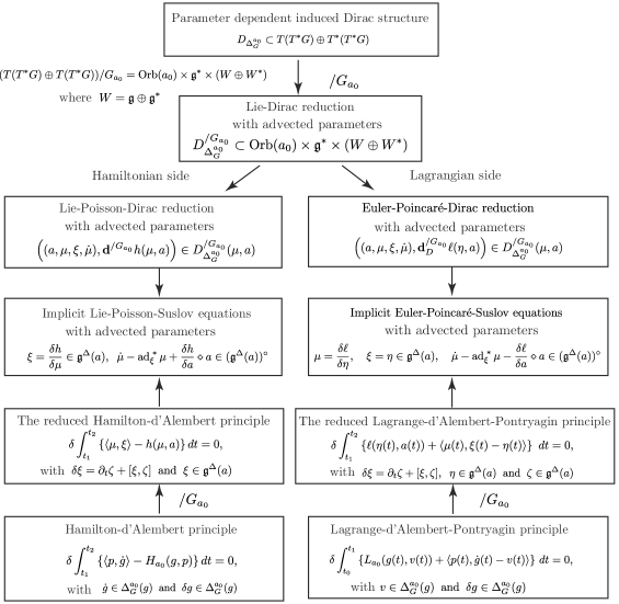
Figure 5.2: Summary of Lie-Dirac reduction with advected parameters

Recall that the equations (5.11) were obtained in (4.25) via the reduced Hamilton-d’Alembert principle with advected quantities. They are here obtained via Dirac reduction.

Recall also that that this system is equivalent to its Lagrangian counterpart (4.10), when the Hamiltonian is associated to the Lagrangian $\ell$ assumed to be hyperregular. This reduction process is however not fully satisfactory on the Hamiltonian side, since one has to assume that the advection equation $\dot{a}+a\xi=0$ holds a priori and one does not obtain it naturally from the reduction approach. However, in order to develop a consistent Dirac reduction approach on the Hamiltonian side, we have to recover, as a particular case, the ordinary Lie-Poisson reduction for semidirect product, that yields directly the advection equation $\dot{a}+a\frac{\delta h}{\delta\mu}=0$ without assuming it a priori.

At first glance, one could think that it is then enough to apply the Lie-Dirac reduction approach developed in Yoshimura, Marsden [2007b] for induced invariant Dirac structures on Lie groups, to the particular case when the Lie group is the semidirect product $S=G\,\circledS\,V$. This is however not the case, as we will mention in details below. In particular, such approach would yield the Lie-Poisson-Suslov equations associated with the semidirect product $\mathfrak{s}=\mathfrak{g}\,\circledS\,V$, which are not the equations (6.15) we aim to obtain, as we already noted in Remark 4.10.

Remark 5.7 (The case of the rolling ball type constraint).

The Dirac reduction approach developed in the present Section evidently applies to the rolling ball type constraints described in §4.3. One starts with the Dirac structure $D_{\Delta^{a_{0}}_{G}}\subset T(T^{*}G)\oplus T^{*}(T^{*}G)$, where $G=K\,\circledS\,V$, and obtains by reduction the Dirac structure $D^{/G_{a_{0}}}_{\Delta_{G}^{a_{0}}}\subset\operatorname{Orb}(a_{0})\times\mathfrak{g}^{\ast}\times W\oplus W^{\ast}$, $W=\mathfrak{g}\times\mathfrak{g}^{\ast}$. We have the equivalence

$$\begin{array}[]{c}\left((a,\mu,b,\xi,X,\rho,\sigma),(a,\mu,b,\beta,\gamma,\eta,Y)\right)\in D^{/G_{a_{0}}}_{\Delta_{G}^{a_{0}}}\\ \Longleftrightarrow\\ \left(\beta+\rho-\operatorname{ad}^{\ast}_{\xi}\mu+X\diamond b,\gamma+\sigma-\xi b\right)\in(\mathfrak{g}^{\Delta}(a))^{\circ}\quad\text{and}\quad(\eta,Y)=(\xi,X)\in\mathfrak{g}^{\Delta}(a).\end{array}$$

The reduced Lagrange-Dirac system reads

$$\left((a,\mu,b,\xi,X,\dot{\mu},\dot{b}),\mathbf{d}_{D}^{/G_{a_{0}}}\ell(a,\eta,Y)\right)\in D^{/G_{a_{0}}}_{\Delta_{G}^{a_{0}}}(a,\mu,b).$$

6 Lie-Dirac reduction for nonholonomic systems on semidirect products

As we already mentioned above, a satisfactory Dirac reduction approach on the Hamiltonian side should extend the properties of the Lie-Poisson reduction for semidirect products. First, the reduced Dirac structure should be obtained, similarly with the Poisson structure, from a Dirac structure on $T^{*}S$, where $S=G\,\circledS\,V$, and not from a Dirac structure on $T^{*}G$ as in the previous section (such approach was however satisfactory for the Lagrangian side). Second, the advection equation for the variable $a$ should be incorporated directly in the reduced geometric object, as in the Poisson case, and not assumed a priori as above (and on the Lagrangian side). In particular, a Dirac reduction by stages should be available in this context, as will be shown later.

Also, contrary to the usual setting in nonholonomic mechanics, one cannot start with the Dirac structure $D_{\Delta_{S}}$ on $T^{*}S$ induced from a given $S$-invariant distribution $\Delta_{S}\subset TS$ via the lifted distribution $\Delta_{T^{\ast}S}=(T\pi_{S})^{-1}\,(\Delta_{S})\subset T(T^{\ast}S)$ since this would yield the Lie-Poisson-Suslov equations on $\mathfrak{s}^{\ast}$ which are not the desired equations in our context. We shall need the Dirac structure associated to another $S$-invariant distribution $\Delta_{T^{*}S}\subset T(T^{*}S)$ constructed from the parameter dependent $G$-invariant distribution $\Delta_{G}(g,a)\subset TG$.

In order to develop this approach systematically, we present below the Lie-Dirac reduction for $S$-invariant Dirac structures on the cotangent bundle of a Lie group $T^{*}S$, induced by an arbitrary distribution $\Delta_{T^{*}S}\subset T(T^{*}S)$ on $T^{*}S$.

6.1 Lie-Dirac reduction: a more general case

In this section, we use the notation $S$ for the Lie group, since later in §6.2, we will apply this reduction to the special case of a semidirect product $S=G\,\circledS\,V$. The results of this section apply to an arbitrary Lie group $S$, not necessarily given by a semidirect product.

Let $\Delta_{T^{*}S}\subset T(T^{*}S)$ be an arbitrary distribution on $T^{*}S$ (not necessarily induced by a distribution on $S$) and consider the Dirac structure $D_{\Delta_{T^{*}}}$ associated with $\Delta_{T^{*}S}\subset T(T^{*}S)$ and the canonical symplectic form, i.e., for each $p_{s}\in T^{\ast}S$,

$$D_{\Delta_{T^{*}S}}(p_{s}) =\left\{(v_{p_{s}},\alpha_{p_{s}})\in T_{p_{s}}(T^{*}S)\oplus T^{*}_{p_{s}}(T^{*}S)\mid v_{p_{s}}\in\Delta_{T^{*}S}(p_{s}),\right.$$

$$\left.\hskip 85.35826pt\left\langle\alpha_{p_{s}},w_{p_{s}}\right\rangle=\Omega(p_{s})\left(v_{p_{s}},w_{p_{s}}\right),\;\;\text{for all}\;\;w_{p_{s}}\in\Delta_{T^{*}S}(p_{s})\right\}.$$

Trivialization.

Let us denote by $\Delta_{S\times\mathfrak{s}^{\ast}}$, the trivialized expression of the distribution $\Delta_{T^{*}S}$. We have $\Delta_{S\times\mathfrak{s}^{\ast}}(s,\mu)\in T_{(s,\mu)}(S\times\mathfrak{s}^{\ast})$, for all $(s,\mu)\in S\times\mathfrak{s}^{\ast}$. The trivialized expression $\bar{D}_{\Delta_{S\times\mathfrak{s}^{\ast}}}\subset T(S\times\mathfrak{s}^{\ast})\oplus T^{*}(S\times\mathfrak{s}^{\ast})$ of the Dirac structure $D_{\Delta_{T^{*}S}}$ reads

$$\bar{D}_{\Delta_{S\times\mathfrak{s}^{\ast}}}(s,\mu) =\left\{\left.\left((v_{s},\rho),(\beta_{s},\eta)\right)\in(T_{s}S\times\mathfrak{s}^{\ast})\oplus(T^{*}_{s}S\times\mathfrak{s})\,\right|\,(v_{s},\rho)\in\Delta_{S\times\mathfrak{s}^{\ast}},\right.$$

$$\;\;\left.\left\langle\beta_{g},w_{g}\right\rangle+\left\langle\eta,\sigma\right\rangle=\omega(s,\mu)\left((v_{s},\rho),(w_{s},\sigma)\right),\;\;\text{for all}\;\;(w_{s},\sigma)\in\Delta_{S\times\mathfrak{s}^{\ast}},\;\sigma\in\mathfrak{s}^{\ast}\right\},$$

where $\omega\in\Omega^{2}(S\times\mathfrak{s}^{\ast})$ is the trivialized canonical symplectic form. We thus have the equivalence

$$\begin{array}[]{c}\left((v_{s},\rho),(\beta_{s},\eta)\right)\in\bar{D}_{\Delta_{S\times\mathfrak{s}^{\ast}}}(s,\mu)\\ \Longleftrightarrow\\ \left(-s\rho+s\operatorname{ad}^{*}_{s^{-1}v_{s}}\mu-\beta_{s},s^{-1}v_{s}-\eta\right)\in\Delta_{S\times\mathfrak{s}^{\ast}}(s,\mu)^{\circ}\quad\text{and}\quad(v_{s},\rho)\in\Delta_{S\times\mathfrak{s}^{\ast}}(s,\mu).\end{array}$$

Reduction.

We suppose that $\Delta_{T^{*}S}$ (and hence $\Delta_{S\times\mathfrak{s}^{\ast}}$) is $S$-invariant. Thus, the distribution is completely determined by $\Delta_{S\times\mathfrak{s}^{\ast}}(e,\mu)\in T_{(e,\mu)}(S\times\mathfrak{s}^{\ast})\cong\mathfrak{s}\times\mathfrak{s}^{\ast}$ and we have $\Delta_{S\times\mathfrak{s}^{\ast}}(s,\mu)=s\Delta_{S\times\mathfrak{s}^{\ast}}(e,\mu)$.

Defining the reduced Dirac structure as usual by $D^{/S}_{{\Delta}_{S\times\mathfrak{s}^{\ast}}}:=\bar{D}_{\Delta_{S\times\mathfrak{s}^{\ast}}}/S$, we get

$$D^{/S}_{{\Delta}_{S\times\mathfrak{s}^{\ast}}}(\mu) =\left\{\left((\mu,\xi,\rho),(\mu,\beta,\eta)\right)\in\mathfrak{s}^{\ast}\times(W\oplus W^{*})\mid(\xi,\rho)\in\Delta_{S\times\mathfrak{s}^{\ast}}(e,\mu),\right.$$

$$\qquad\left.\left\langle\beta,\zeta\right\rangle+\left\langle\eta,\sigma\right\rangle=\left\langle\sigma,\xi\right\rangle-\left\langle\rho,\zeta\right\rangle+\left\langle\mu,[\xi,\zeta]\right\rangle,\;\;\text{for all}\;\;(\zeta,\sigma)\in\Delta_{S\times\mathfrak{s}^{\ast}}(e,\mu)\right\},$$

where $W=\mathfrak{s}\times\mathfrak{s}^{\ast}$. We thus have the equivalence

$$\begin{array}[]{c}\left((\mu,\xi,\rho),(\mu,\beta,\eta)\right)\in D^{/S}_{{\Delta}_{S\times\mathfrak{s}^{\ast}}}(\mu)\\ \Longleftrightarrow\\ \left(-\rho+\operatorname{ad}^{*}_{\xi}\mu-\beta,\xi-\eta\right)\in\left({\Delta}_{S\times\mathfrak{s}^{\ast}}(e,\mu)\right)^{\circ}\quad\text{and}\quad(\xi,\rho)\in\Delta_{G\times\mathfrak{s}^{\ast}}(e,\mu).\end{array}$$ (6.1)

Equations of motions.

Let $H:T^{*}S\rightarrow\mathbb{R}$ be a Hamiltonian function. The Hamilton-Dirac system

$$\left((s,p,\dot{s},\dot{p}),\mathbf{d}H(s,p)\right)\in D_{\Delta_{T^{*}S}}(s,p)$$

yields locally the conditions

$$(\dot{s},\dot{p})\in\Delta_{T^{*}S}(s,p),\quad\left(\frac{\partial H}{\partial s}+\dot{p},\frac{\partial H}{\partial p}-\dot{s}\right)\in\Delta_{T^{*}S}(s,p)^{\circ}.$$ (6.2)

Assuming that $H$ is $S$-invariant and proceeding as in §2.6, we get the reduced Hamilton-Dirac system

$$((\mu,\xi,\dot{\mu}),(\mathbf{d}^{/S}h(\mu))\in D^{/S}_{{\Delta}_{S\times\mathfrak{s}^{\ast}}}(\mu),$$

where $\mathbf{d}^{/S}h:=(\overline{\mathbf{d}H})^{/S}:\mathfrak{s}^{\ast}\rightarrow\mathfrak{s}^{\ast}\times(\mathfrak{s}^{\ast}\oplus\mathfrak{s})$ is given by $\mathbf{d}^{/S}h(\mu)=\left(\mu,0,\frac{\delta{h}}{\delta{\mu}}\right)$. We thus get the equations

$$\left(-\dot{\mu}+\operatorname{ad}^{*}_{\xi}\mu,\xi-\frac{\delta h}{\delta\mu}\right)\in{\Delta}_{S\times\mathfrak{s}^{\ast}}(e,\mu)^{\circ}\quad\text{and}\quad(\xi,\dot{\mu})\in\Delta_{S\times\mathfrak{s}^{\ast}}(e,\mu).$$ (6.3)

Remark 6.1 (Recovering the case of the lifted distribution).

In the particular case when $\Delta_{T^{*}S}$ is the lifted distribution associated to a given $S$-invariant distribution $\Delta_{S}\subset TS$, that is, $\Delta_{T^{*}S}=\left(T\pi\right)^{-1}(\Delta_{S})$, we have ${\Delta}_{S\times\mathfrak{s}^{\ast}}=\mathfrak{s}^{\Delta}\times\mathfrak{s}^{\ast}$ and thus $({\Delta}_{S\times\mathfrak{s}^{\ast}})^{\circ}=\left(\mathfrak{s}^{\Delta}\right)^{\circ}\times\{0\}$, so that (6.1) consistently recovers

$$\beta+\rho-\operatorname{ad}^{*}_{\xi}\mu\in(\mathfrak{s}^{\Delta})^{\circ},\quad\eta=\xi\in\mathfrak{s}^{\Delta}$$

and hence (6.3) recovers the implicit Lie-Poisson-Suslov equations (2.18):

$$\dot{\mu}-\operatorname{ad}^{*}_{\xi}\mu\in(\mathfrak{s}^{\Delta})^{\circ},\quad\frac{\delta h}{\delta\mu}=\xi\in\mathfrak{s}^{\Delta}.$$

6.2 Lie-Dirac reduction by stages on semidirect products

We now apply the Lie-Dirac reduction described in §6.1 to the particular case when the Lie group $S$ is the semidirect product $S=G\,\circledS\,V$. We then show that by choosing an appropriate $S$-invariant distribution $\Delta_{T^{*}S}\subset T(T^{*}S)$ constructed from the $G$-invariant and parameter dependent distribution $\Delta_{G}(g,a)\subset TG$, we recover an implicit version of the nonholonomic Lie-Poisson equations that naturally includes the advection equation, without having to formulate it as an hypothesis. In order to illustrate the analogy with the usual Poisson reduction for semidirect products (see Theorem 3.2 and Remark 3.3) our approach will be done using a reduction by stages. We first reduce by the normal subgroup $V$ of $S$, and then by $G=S/V$.

The case of an arbitrary invariant distribution.

In order to find the appropriate $S$-invariant distribution needed on $T^{*}S$, we first consider an arbitrary $S$-invariant distribution $\Delta_{T^{*}S}\subset T(T^{*}S)$ and its associated Dirac structure, for $(g,p,u,a_{0})\in T^{*}G\times T^{\ast}V\cong T^{\ast}S$,

$$D_{\Delta_{T^{*}S}}(g,p,u,a_{0})\subset T_{(g,p,u,a_{0})}T^{*}S\oplus T^{*}_{(g,p,u,a_{0})}T^{*}S.$$

Note that here $a_{0}$ denotes an arbitrary element in $V^{\ast}$ and is not fixed. Given a Hamiltonian $H:T^{*}S\rightarrow\mathbb{R}$, we know from (6.2) that the associated Hamilton-Dirac system

$$\left((g,p,\dot{g},\dot{p},u,a_{0},\dot{u},\dot{a}_{0}),\mathbf{d}H(g,p,u,a_{0})\right)\in D_{\Delta_{T^{*}S}}(g,p,u,a_{0}),$$

yields locally the conditions

$$(\dot{g},\dot{p},\dot{u},\dot{a}_{0})\in\Delta_{T^{*}S},\quad\left(\frac{\partial H}{\partial g}+\dot{p},\frac{\partial H}{\partial u}+\dot{a}_{0},\frac{\partial H}{\partial p}-\dot{g},\frac{\partial H}{\partial a_{0}}-\dot{u}\right)\in\left(\Delta_{T^{*}S}\right)^{\circ}.$$ (6.4)

As before, let us denote by $\bar{D}_{\Delta_{S\times\mathfrak{s}^{\ast}}}$ the trivialized Dirac structure induced on $S\times\mathfrak{s}^{\ast}$. From (6.3), we know that a reduction by $S$ yields the Dirac system

$$\left((\mu,a,\xi,v,\dot{\mu},\dot{a}),\mathbf{d}^{/S}h(\mu,a)\right)\in D^{/S}_{\Delta_{S\times\mathfrak{s}^{\ast}}}(\mu,a)$$ (6.5)

with the associated equations

$$\left(-(\dot{\mu},\dot{a})+\operatorname{ad}^{*}_{(\xi,v)}(\mu,a),(\xi,v)-\left(\frac{\delta h}{\delta\mu},\frac{\delta h}{\delta a}\right)\right)\in\Delta_{S\times\mathfrak{s}^{\ast}}(e,0,\mu,a)^{\circ}$$

and

$$(\mu,a,\xi,v,\dot{\mu},\dot{a})\in\Delta_{S\times\mathfrak{s}^{\ast}}(e,0,\mu,a).$$

Definition of the distribution on $T^{*}S$.

In order to recover from (6.5) the implicit Lie-Poisson-Suslov equations (4.25) together with the advection equation $\partial_{t}a+\xi a=0$, we need to choose the $S$-invariant distribution $\Delta_{T^{*}S}\subset T(T^{*}S)$ in such a way that the equality

$$\Delta_{S\times\mathfrak{s}^{\ast}}(e,0,\mu,a)=\mathfrak{g}^{\Delta}(a)\times T_{0}V\times T_{(\mu,a)}\mathfrak{s}^{\ast}\subset T_{(e,0,\mu,a)}(S\times\mathfrak{s}^{\ast})$$ (6.6)

holds. By $S$-invariance, this means that, at $(g,u,\mu,a)\in S\times\mathfrak{s}^{\ast}$, we have

$$\Delta_{S\times\mathfrak{s}^{\ast}}(g,u,\mu,a) =(g,u)\left(\mathfrak{g}^{\Delta}(a)\times T_{0}V\times T_{(\mu,a)}\mathfrak{s}^{\ast}\right)$$

$$=\Delta_{G}(g,ga)\times T_{u}V\times T_{(\mu,a)}\mathfrak{s}^{\ast}\subset T_{(g,u,\mu,a)}(S\times\mathfrak{s}^{\ast}).$$

Using the expression for the trivialization $T^{*}S\rightarrow S\times\mathfrak{s}^{\ast}$ given by,

$$(g,p,u,a_{0})\in T^{*}S$$

$$\quad\mapsto(g,u,\mu,a)=\left((g,u),(g,u)^{-1}(g,p,u,a_{0})\right)=\left((g,u),g^{-1}p,g^{-1}a_{0}\right)\in S\times\mathfrak{s}^{\ast},$$

we obtain that $\Delta_{T^{*}S}$ has to be defined as follows.

Definition 6.2.

The distribution $\Delta_{T^{*}S}\subset T(T^{*}S)$ on $T^{*}S$ associated to a given constraint distribution $\Delta_{G}^{a_{0}}\subset TG$ on $G$ is defined as

$$\Delta_{T^{*}S}:=(T\pi_{S})^{-1}(\Delta^{a_{0}}_{G}\times TV)=\left((T\pi_{G})^{-1}\Delta_{G}^{a_{0}}\right)\times T(T^{*}V).$$ (6.7)

In more details, we have

$$\Delta_{T^{*}S}(g,p,u,a_{0}) =\left(T_{(g,p,u,a_{0})}\pi_{S}\right)^{-1}\left(\Delta_{G}^{a_{0}}(g)\times T_{u}V\right)$$

$$=\left(\left(T_{(g,p)}\pi_{G}\right)^{-1}\left(\Delta_{G}^{a_{0}}(g)\right)\right)\times T_{(u,a_{0})}T^{*}V\subset T_{(g,p,u,a_{0})}T^{*}S,$$

where it is important to note that the vector space $\Delta_{T^{*}S}(g,p,u,a_{0})$ depends on $a_{0}\in V^{\ast}$. In this case, the implicit Hamiltonian system (6.4) reads

$$\dot{g}\in\Delta_{G}^{a_{0}}(g),\quad\frac{\partial H}{\partial g}+\dot{p}\in\Delta_{G}^{a_{0}}(g)^{\circ},\quad\frac{\partial H}{\partial u}+\dot{a}_{0}=0,\quad\frac{\partial H}{\partial p}-\dot{g}=0,\quad\frac{\partial H}{\partial a_{0}}-\dot{u}=0.$$

Dirac reduction by stages: first stage.

The first stage reduction consists in reducing the Dirac structure by the normal subgroup $V$ of $S$. We note that the subgroup action of $w\in V$ on $S$ and $T^{*}S$ reads

$$w(g,u)=(g,w+u),\quad\text{and}\quad w(g,p,u,a_{0})=(g,p,w+u,a_{0}).$$

It follows that the Hamiltonian $H:T^{*}S\rightarrow\mathbb{R}$, $H=H(g,p,u,a_{0})$ is $V$-invariant if and only if it does not depend on the variable $u$. Similarly, $\Delta_{T^{*}S}$ is $V$-invariant if and only if the vector space $\Delta_{T^{*}S}(g,p,u,a_{0})$ does not depend on the variable $u$. For such a Hamiltonian, we have

$$\mathbf{d}H:T^{*}S\rightarrow T(T^{*}S),\quad\mathbf{d}H(g,p,u,a_{0})=\left(g,p,\frac{\partial H}{\partial g},\frac{\partial H}{\partial p},u,a_{0},0,\frac{\partial H}{\partial a_{0}}\right).$$

Using the equalities

$$T^{*}S/V=T^{*}G\times V^{*},\quad T(T^{*}S)/V=T(T^{*}G)\times V^{*}\times V\times V^{\ast}$$

$$T^{*}(T^{*}S)/V=T^{*}(T^{*}G)\times V^{*}\times V^{*}\times V,$$

we obtain the reduced derivative $\mathbf{d}^{/V}H:T^{*}G\times V^{*}\rightarrow T^{*}(T^{*}G)\times V^{*}\times V^{*}\times V$

$$\mathbf{d}^{/V}H(g,p,a_{0})=\left(g,p,\frac{\partial H}{\partial g},\frac{\partial H}{\partial p},a_{0},0,\frac{\partial H}{\partial a_{0}}\right).$$

Note that we have the equality

$$\left(T(T^{*}S)\oplus T^{*}(T^{*}S)\right)/V=T(T^{*}G)\times V^{*}\times V\times V^{*}\oplus T^{*}(T^{*}G)\times V^{*}\times V^{*}\times V$$

as vector bundles over $T^{*}G\times V^{*}$.

Since both $\Delta_{T^{*}S}$ and the canonical symplectic form on $T^{*}S$ do not depend on $u$, the fiber $D_{\Delta_{T^{*}S}}(g,p,u,a_{0})$ of the associated Dirac structure $D_{\Delta_{T^{*}S}}$ does not depend on $u$, either. Therefore, since the $V$-action does not affect the vector fibers above $T^{*}S$, the reduced Dirac structure $D^{/V}_{\Delta_{T^{*}S}}:=\left(D_{\Delta_{T^{*}S}}\right)/V$, with

$$D^{/V}_{\Delta_{T^{*}S}}(g,p,a_{0})\subset T_{(p,g)}(T^{*}G)\times\{a_{0}\}\times V\times V^{*}\oplus T^{*}_{(g,p)}(T^{*}G)\times\{a_{0}\}\times V^{*}\times V,$$ (6.8)

has the same expression as the Dirac structure $D_{\Delta_{T^{*}S}}$.

The reduced Hamilton-Dirac system reads

$$\left((g,p,\dot{g},\dot{p},a_{0},\dot{u},\dot{a}_{0}),\mathbf{d}^{/V}H(g,p,a_{0})\right)\in D^{/V}_{\Delta_{T^{*}S}}(g,p,a_{0})$$

and the associated equations are

$$(\dot{g},\dot{p},\dot{u},\dot{a}_{0})\in\Delta_{T^{*}S}^{/V}(g,p,a_{0}),\quad\left(\frac{\partial H}{\partial g}+\dot{p},\dot{a}_{0},\frac{\partial H}{\partial p}-\dot{g},\frac{\partial H}{\partial a_{0}}-\dot{u}\right)\in\Delta^{/V}_{T^{*}S}(g,p,a_{0})^{\circ},$$

where $(g,p,a_{0})\in T^{*}G\times V^{*}$, and we denote by $\Delta_{T^{*}S}^{/V}(g,p,a_{0})$ the quotient of $\Delta_{T^{*}S}(g,p,u,a_{0})$, in which $\Delta_{T^{*}S}$ does not depend on the variable $u\in V$.

For the particular case in which the distribution $\Delta_{T^{*}S}\subset T(T^{*}S)$ is induced by the distribution $\Delta_{G}^{a_{0}}\subset TG$ via (6.7), the equations are

$$\dot{g}\in\Delta_{G}^{a_{0}}(g),\quad\frac{\partial H}{\partial g}+\dot{p}\in\Delta_{G}^{a_{0}}(g)^{\circ},\quad\dot{a}_{0}=0,\quad\frac{\partial H}{\partial p}-\dot{g}=0,\quad\frac{\partial H}{\partial a_{0}}-\dot{u}=0.$$

Since $\dot{a}_{0}=0$, and $H$ does not depend on $u$, the last equation decouples from the others, and the first four equations are equivalent to the implicit Hamilton-d’Alembert equations (5.9) for $H_{a_{0}}$.

Dirac reduction by stages: second stage.

The expression of the reduced Dirac structure $D^{/S}_{\Delta_{T^{*}S}}$ can be either obtained by reducing the Dirac structure $D^{/V}_{\Delta_{T^{*}S}}$ by the group $G$, or by reducing the Dirac structure $D_{\Delta_{T^{*}S}}$ by the group $S$. This follows from the fact that $V$ is a normal subgroup of $S=G\,\circledS\,V$. We shall explain the reduction of $D_{\Delta_{T^{*}S}}$ by $S$ in the following.

By applying the general result obtained in (6.1) for $S$ to the semidirect product $S=G\,\circledS\,V$, we obtain the following description of the reduced Dirac structure $D^{/S}_{\Delta_{T^{*}S}}\subset\mathfrak{s}^{\ast}\times(W\oplus W^{\ast})$, with $W=\mathfrak{s}\times\mathfrak{s}^{\ast}$:

$$\begin{array}[]{c}\left((\mu,a,\xi,w,\rho,b),(\mu,a,\beta,c,\eta,v)\right)\in D^{/S}_{{\Delta}_{S\times\mathfrak{s}^{\ast}}}(\mu,a)\\ \Longleftrightarrow\\ \left(-(\rho,b)+\operatorname{ad}^{*}_{(\xi,w)}(\mu,a)-(\beta,c),(\xi,w)-(\eta,v)\right)\in{\Delta}_{S\times\mathfrak{s}^{\ast}}(e,\mu)^{\circ}\\ \text{and}\quad(\xi,w,\rho,b)\in\Delta_{S\times\mathfrak{s}^{\ast}}(e,0,\mu,a),\\ \Longleftrightarrow\\ -\rho+\operatorname{ad}^{*}_{\xi}\mu-w\diamond a-\beta\in(\mathfrak{g}^{\Delta}(a))^{\circ},\;\;b+\xi a+c=0,\;\;\xi=\eta,\;\;w=v,\quad\xi\in\mathfrak{g}^{\Delta}(a),\end{array}$$ (6.9)

where in the second equivalence we used $\Delta_{S\times\mathfrak{s}^{\ast}}(e,0,\mu,a)=\mathfrak{g}^{\Delta}(a)\times T_{0}V\times T_{(\mu,a)}\mathfrak{s}^{\ast}$, see (6.6), and $\Delta_{S\times\mathfrak{s}^{\ast}}(e,0,\mu,a)^{\circ}=(\mathfrak{g}^{\Delta}(a))^{\circ}\times\{0\}\times\{0\}$, as well as the expression of the operator $\operatorname{ad}^{*}$ for the semidirect product.

From (6.9) it follows that the solution curves of the reduced Hamilton-Dirac system

$$\left((\mu,a,\xi,w,\dot{\mu},\dot{a}),\mathbf{d}^{/S}h(\mu,a)\right)\in D^{/S}_{\Delta_{S\times\mathfrak{s}^{\ast}}}(\mu,a)$$

verify the equations

$$\dot{\mu}-\operatorname{ad}^{*}_{\xi}\mu+w\diamond a\in(\mathfrak{g}^{\Delta}(a))^{\circ},\;\;\dot{a}+\xi a=0,\;\;\xi=\frac{\delta h}{\delta\mu},\;\;w=\frac{\delta h}{\delta a},\;\;\xi\in\mathfrak{g}^{\Delta}(a).$$

These are exactly the desired equations, namely, the implicit Lie-Poisson version of the Euler-Poincaré-Suslov equations (4.10) (compare with (5.11)) which contains in addition the advection equation for the advected parameter $a$.

As we already mentioned, these equations cannot be obtained by reduction of the $S$-invariant Dirac structure in $T(T^{*}S)\oplus T^{*}(T^{*}S)$ induced by a distribution $\Delta_{S}\subset TS$. Indeed, we had to use the Dirac structure induced by the distribution $\Delta_{T^{*}S}\subset T(T^{*}S)$ given in (6.7), which is not of the lifted from $\left(T\pi\right)^{-1}(\Delta_{S})$.

The results obtained in this section are briefly summarized in the following theorem.

Theorem 6.3.

Let $\Delta_{G}^{a_{0}}\subset TG$, $a_{0}\in V^{\ast}$ be a family of constraint distributions on $G$ such that $\Delta_{G}(hg,ha)=h\Delta_{G}(g,a)$, for all $h\in G$. Consider the semidirect product $S=G\,\circledS\,V$ and let $\Delta_{T^{*}S}$ be the distribution on $T^{*}S$ associated with $\Delta_{G}^{a_{0}}$, as defined in (6.7). Let $H:T^{*}S\rightarrow\mathbb{R}$ be a $S$-invariant Hamiltonian and let $h:\mathfrak{s}^{\ast}\rightarrow\mathbb{R}$ be the associated reduced Hamiltonian. Then we have the following results.

• The distribution $\Delta_{T^{*}S}$ and the associated Dirac structure $D_{\Delta_{T^{*}S}}$ on $T^{*}S$ are $S$-invariant.

• The first stage reduction yields the reduced Dirac structure $D^{/V}_{\Delta_{T^{*}S}}$ given in (6.8) on the first stage reduced Pontryagin bundle $(T(T^{*}S)\oplus T^{*}(T^{*}S))/V$.

• The solution curves of the reduced Hamilton-Dirac system associated to $D^{/V}_{\Delta_{T^{*}S}}$ verify the implicit Hamilton-d’Alembert equations

  $$\dot{g}\in\Delta_{G}^{a_{0}}(g),\quad\frac{\partial H}{\partial g}+\dot{p}\in\Delta_{G}^{a_{0}}(g)^{\circ},\quad\dot{a}_{0}=0,\quad\frac{\partial H}{\partial p}-\dot{g}=0,\quad\frac{\partial H}{\partial a_{0}}-\dot{u}=0.$$

• The second stage reduction, namely the reduction of $D^{/V}_{\Delta_{T^{*}S}}$ by $G$, yields the reduced Dirac structure $D^{/S}_{\Delta_{T^{*}S}}$ given in (6.9) on the second stage reduced Pontryagin bundle $(T(T^{*}S)\oplus T^{*}(T^{*}S))/V/G=(T(T^{*}S)\oplus T^{*}(T^{*}S))/S$. This follows from the fact that $V$ is a normal subgroup of $S=G\,\circledS\,V$.

• The solution curves of the reduced Hamilton-Dirac system associated to $D^{/S}_{\Delta_{T^{*}S}}$ verify the implicit Lie-Poisson-Suslov equations with advected parameters together with the advection equation

  $$\dot{\mu}-\operatorname{ad}^{*}_{\xi}\mu+w\diamond a\in\left(\mathfrak{g}^{\Delta}(a)\right)^{\circ},\quad\dot{a}+\xi a=0,\quad\xi=\frac{\delta h}{\delta\mu},\quad w=\frac{\delta h}{\delta a},\quad\xi\in\mathfrak{g}^{\Delta}(a).$$

Figure 6.1: Dirac reduction by stages for semidirect products

6.3 Relation with the Lagrange-Dirac side

The aim of this section is to relate the Dirac structure $D_{\Delta_{T^{*}S}}\subset T(T^{*}S)\oplus T^{*}(T^{*}S)$ defined above for the Hamiltonian side and the family of Dirac structures with parameter $D_{\Delta^{a_{0}}}\subset T(T^{*}G)\oplus T^{*}(T^{*}G)$ used in the Lagrangian side and in §5.3, by using exclusively a Dirac reduction point of view.

Recall that in the standard case of Hamiltonian and Lagrangian dynamics, which corresponds to the choice of the canonical Dirac structure, one passes from the canonical Hamiltonian description associated to $\bar{H}$ on $T^{*}S$ to the canonical Hamilton description associated to $H_{a_{0}}$ on $T^{*}G$ by a symplectic reduction by the subgroup $V$ at the particular value $a_{0}\in V^{\ast}$ of the momentum map $\mathbf{J}_{V}:T^{*}S\rightarrow V^{\ast}$. From the Dirac point of view, this means that one has to reduce the canonical Dirac structure on $T^{*}S$ in order to get the canonical Dirac structure on $T^{*}G$. The reduction approach that has to be used here to relate the noncanonical Dirac structures $D_{\Delta_{T^{*}S}}$ and $D_{\Delta^{a_{0}}_{G}}$ is therefore the one that parallels symplectic reduction, as developed in Blankenstein, van der Schaft [2001].

Roughly speaking the reduction process goes as follows. Given a Dirac structure $D$ on a manifold $M$ and a free and proper Lie group action of $G$ on $M$, one first assumes that the action admits an equivariant momentum map relative to $D$, that is, there exists a $G$-equivariant map $\mathbf{J}:M\rightarrow\mathfrak{g}^{\ast}$ such that $(\xi_{M},\mathbf{d}\mathbf{J}_{\xi})\in D$, for all $\xi\in\mathfrak{g}$. The process goes in two steps.

First, if $\mu\in\mathfrak{g}^{\ast}$ is a regular value of $\mathbf{J}$ then $M_{\mu}:=\mathbf{J}^{-1}(\mu)\subset M$ is a submanifold. If the dimension of the vector subspaces $D(m)\cap(T_{m}{M_{\mu}}\times T^{*}_{m}M|_{M_{\mu}})\subset T_{m}M_{\mu}\times T^{*}_{m}M|_{M_{\mu}}$ is independent of $m\in M_{\mu}$, then these vector spaces naturally induce a Dirac structure $D_{M_{\mu}}\subset TM_{\mu}\oplus T^{*}M_{\mu}$.

Second, one observes that the Dirac structure $D_{M_{\mu}}$ is $G_{\mu}$-invariant, where $G_{\mu}=\{g\in G\mid\operatorname{Ad}^{*}_{g}\mu=\mu\}$ is the coadjoint isotropy subgroup of $\mu$. Under appropriate conditions (we do not detail them because they are trivially satisfied in our example, and refer to Blankenstein, van der Schaft [2001]), one obtains a reduced Dirac structure $D_{\mu}\subset T(M_{\mu}/G_{\mu})\oplus T^{\ast}(M_{\mu}/G_{\mu})$ on $M_{\mu}/G_{\mu}=\mathbf{J}^{-1}(\mu)/G_{\mu}$ described in terms of its local sections by

$$(\mathfrak{D}_{\mu})_{loc}: =\{(X,\alpha)\in\mathfrak{X}_{loc}(M_{\mu}/G_{\mu})\times\Omega^{1}_{loc}(M_{\mu}/G_{\mu})\mid\exists\,(Y,\beta)\in\mathfrak{D}_{loc},$$ (6.10)

$$\qquad\qquad\qquad\qquad\qquad\qquad\;\text{such that}\;T\pi\circ Y=X\circ\pi,\;\pi^{\ast}\alpha=\beta\},$$

see Blankenstein, van der Schaft [2001].

We shall now apply this reduction approach to the Dirac structure associated to

$$\Delta_{T^{*}S}(g,p,u,a_{0})=\left(T_{(g,p,u,a_{0})}\pi\right)^{-1}\left(\Delta_{G}^{a_{0}}(g)\times T_{u}V\right)=\left(T_{(g,p)}\pi_{G}\right)^{-1}(\Delta^{a_{0}}(g))\times T_{(u,a_{0})}T^{*}V$$

on $T^{*}S$. Note that in general, if $\mathbf{J}:P\rightarrow\mathfrak{g}^{\ast}$ is a momentum map for a symplectic action of $G$ on the symplectic vector space $(P,\omega)$, and if one considers the Dirac structure $D$ associated with $\omega$ and a distribution $\Delta\subset TP$ as in (2.6), then $\mathbf{J}$ is also a Dirac momentum map, provided we have $\xi_{P}(x)\in\Delta(x)$, for all $x\in P$ and $\xi\in\mathfrak{g}$. In our case, this hypothesis is verified since the $V$ action on $T^{*}S$ reads $(g,p,u,a_{0})\mapsto(g,p,u+w,a_{0})$, so the infinitesimal generator $w_{V}$ at $(g,p,u,a_{0})$ is given by $(0,0,w,0)$ which belongs to $\Delta_{T^{*}M_{\mu}}(g,p,u,a_{0})$. Choosing a momentum value $a_{0}\in V^{\ast}$, we have $\mathbf{J}_{V}^{-1}(a_{0})=T^{*}G\times V\times\{a_{0}\}\simeq T^{*}G\times V$.

According to the process recalled above, the Dirac structure obtained on $T^{*}G\times V$ is given by

$$\left(D_{\Delta_{T^{*}S}}\right)_{T^{*}G\times V}(g,p,u)$$

$$\quad=D_{\Delta_{T^{*}S}}(g,p,u,a_{0})\cap\left(T_{(g,p,u)}(T^{*}G\times V)\times T^{*}_{(g,p,u)}(T^{*}(G\times V)|_{T^{*}G\times V})\right),$$ (6.11)

where we recall that $a_{0}\in V^{\ast}$ is fixed and we note that the dimension condition is verified. First we observe that

$$\left((g,p,u,a_{0},\dot{g},\dot{p},\dot{u},\dot{a}_{0}),(g,p,u,a_{0},\alpha,v,b,w)\right)\in D_{\Delta_{T^{*}S}}(g,p,u,a_{0})$$

if and only if $(g,p,u,a_{0},\dot{g},\dot{p},\dot{u},\dot{a}_{0})\in\Delta_{T^{*}S}$ and $(g,p,u,a_{0},\alpha+\dot{p},v-\dot{g},b+\dot{a}_{0},w-\dot{u})\in\Delta_{T^{*}S}^{\circ}$, which is equivalent to $(g,\dot{g})\in\Delta^{a_{0}}(g)$, $\alpha+\dot{p}\in\Delta^{a_{0}}(g)^{\circ}$, $v=\dot{g}$, $b+\dot{a}_{0}=0$, $w=\dot{u}$. Formula (6.3) means that in addition we have $\dot{a}_{0}=0$ and $w=0$. So we deduce that

$$\left(D_{\Delta_{T^{*}S}}\right)_{T^{*}G\times V}(g,p,u)$$

$$=\{(g,p,u,\dot{g},\dot{p},\dot{u}),(g,p,u,\alpha,v,b)\in T_{(g,p,u)}(T^{*}G\times V)\oplus T^{\ast}_{(g,p,u)}(T^{*}G\times V)\mid$$ (6.12)

$$\qquad\qquad\qquad\qquad\qquad\qquad\qquad\qquad\qquad\qquad((g,p,\dot{g},\dot{p}),(g,p,\alpha,v))\in D_{\Delta^{a_{0}}_{G}}\}.$$

To carry out the second step, we recall that the isotropy group is $V_{a_{0}}=V$ and that $(T^{*}G\times V)/V=T^{*}G$. Then, a direct application of formula (6.10) to the Dirac structure (6.3) shows that the reduced Dirac structure is given by $D_{\Delta^{a_{0}}_{G}}\subset T(T^{*}G)\oplus T^{*}(T^{*}G)$. We thus have obtained the following result.

Theorem 6.4.

The Dirac structure $D_{\Delta_{G}^{a_{0}}}\subset T(T^{*}G)\oplus T^{*}(T^{*}G)$ associated to the nonholonomic constraint $\Delta_{G}^{a_{0}}\subset TG$ is obtained from the $S$-invariant Dirac structure $D_{\Delta_{T^{*}S}}\subset T(T^{*}S)\oplus T^{*}(T^{*}S)$ defined in (6.7) by the Dirac reduction process of Blankenstein, van der Schaft [2001] with respect to the momentum value $a_{0}\in V^{\ast}$.

The relation between the various Dirac reductions involved is illustrated in the following diagram.

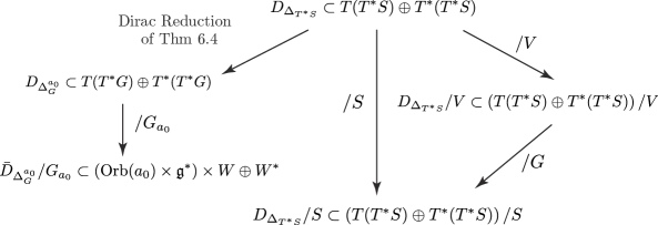
Figure 6.2: Relation between Dirac reductions

6.4 The Hamilton-d’Alembert principle in phase space

We shall now develop the Hamilton-d’Alembert principle in phase space naturally associated to the approach presented in §6.2. It extends the Hamilton-d’Alembert principle developed in §4.5 in the sense that it naturally implies the advection equation without having to assume it a priori.

In order to obtain this principle, it suffices to consider the Hamilton-d’Alembert principle in phase space $T^{*}S\cong T^{*}G\times T^{\ast}V$ (instead of $T^{*}G$ as in §4.5) for a Hamiltonian $\bar{H}=\bar{H}(g,p,u,a_{0}):T^{*}S\rightarrow\mathbb{R}$, and with constraint distribution $\Delta^{a_{0}}_{G}(g)\times T_{u}V\subset TS$ (see, (6.7)). Note that this principle is slightly more general than the Hamilton-d’Alembert principle for nonholonomic mechanics developed in §4.5, since the distribution constraint also depends on the fiber in $T^{*}S$ ($a_{0}$, here) and not only on the base point $(g,u)\in S$.

The principle thus reads

$$\delta\int_{t_{1}}^{t_{2}}\left\{\left\langle p,\dot{g}\right\rangle+\left\langle a_{0},\dot{u}\right\rangle-\bar{H}(g,p,u,a_{0})\right\}dt=0,\quad(\dot{g},\dot{u})\in\Delta_{G}^{a_{0}}\times T_{u}V,$$ (6.13)

for arbitrary variations $(\delta g(t),\delta p(t),\delta u(t),\delta a_{0}(t))$ of the curve $(g(t),p(t),u(t),a_{0}(t))$ in $T^{\ast}S$, with $\delta g(t)$ and $\delta u(t)$ vanishing at the endpoints and $(\delta g,\delta{u})\in\Delta_{G}^{a_{0}}\times T_{u}V$.

In our context, the Hamiltonian $\bar{H}$ is $S$-invariant and, in particular, does not depend on $u$ and is related to the given Hamiltonian function $H$ via the simple relation $\bar{H}(g,p,u,a_{0})=H(g,p,a_{0})$, see Remark 3.3. A similar proof as before, yields the following theorem.

Theorem 6.5.

Let $\bar{H}:T^{*}S\rightarrow\mathbb{R}$ be a $S$-invariant Hamiltonian and let $\Delta^{a_{0}}_{G}\subset TG$ be a family of distribution verifying the $G$-invariance assumption (4.6). Consider a curve $(g(t),p(t),u(t),a_{0}(t))\in T^{*}S$, $t\in[t_{1},t_{2}]$, and define the curves $\mu(t)=g(t)^{-1}p(t)$ and $a(t)=g(t)^{-1}a_{0}$. Then the following are equivalent.

• The Hamilton-d’Alembert principle in phase space

  $$\delta\int_{t_{1}}^{t_{2}}\left\{\left\langle p,\dot{g}\right\rangle+\left\langle a_{0},\dot{u}\right\rangle-\bar{H}(g,p,u,a_{0})\right\}dt=0,\quad(\dot{g},\dot{u})\in\Delta^{a_{0}}_{G}(g)\times T_{u}V\subset TS$$

  holds, for variations $(\delta g(t),\delta u(t))$ of $(g(t),u(t))$ vanishing at the endpoints and such that $(\delta g,\delta{u})\in\Delta^{a_{0}}_{G}(g)\times T_{u}V$, and for arbitrary variations $(\delta p(t),\delta a_{0}(t))$ of $(p(t),a_{0}(t))$.

• The curve $(g(t),p(t),u(t),a_{0}(t))\in T^{*}S$, $t\in[t_{1},t_{2}]$ satisfies the implicit Hamiltonian system with constraint:

  $$\dot{p}+\frac{\partial\bar{H}}{\partial g}\in\Delta_{G}(g)^{\circ},\quad\dot{g}=\frac{\partial\bar{H}}{\partial p}\in\Delta_{G}(g),\quad\dot{a}_{0}=0,\quad\dot{u}=\frac{\partial\bar{H}}{\partial a_{0}}.$$

• The reduced Hamilton-d’Alembert principle with advected quantities

  $$\delta\int_{t_{1}}^{t_{2}}\left\{\left\langle\mu,\xi\right\rangle+\left\langle a,v\right\rangle-h(\mu,a)\right\}dt=0,\quad\xi\in\mathfrak{g}^{\Delta}(a)$$ (6.14)

  holds, for arbitrary variations $\delta\mu(t)$, $\delta a(t)$ and variations $\delta\xi(t)$ and $\delta v(t)$ of the form $\delta\xi=\partial_{t}\zeta+[\xi,\zeta]$ and $\delta v=\partial_{t}w+\xi w-\zeta v$, where $\zeta\in\mathfrak{g}^{\Delta}(a)$ vanishes at the endpoints and $w\in V$ is arbitrary and vanishes at endpoints.

• The implicit Lie-Poisson-Suslov equations with parameters, together with the advection equation

  $$\xi=\frac{\delta h}{\delta\mu},\quad v=\frac{\delta h}{\delta{a}},\quad\xi\in\mathfrak{g}^{\Delta}(a),\quad\dot{\mu}-\operatorname{ad}_{\xi}^{\;\ast}\mu+v\diamond a\in\left(\mathfrak{g}^{\Delta}(a)\right)^{\circ},\quad\dot{a}+a\xi=0$$ (6.15)

  hold.

Remark 6.6.

It is important to compare the four points of the previous theorem with the four points of Theorem 4.8, and also to note that in Theorem 6.5, the advection equation is a consequence of the reduced Hamilton-d’Alembert principle with advected quantities. While Theorem 4.8 is associated to the Dirac reduction approach of §4.5 which starts with the Dirac structure $D_{\Delta^{a_{0}}_{G}}$ on $T^{*}G$, Theorem 6.5 is associated with the Dirac reduction approach §6 which starts with the Dirac structure $D_{\Delta_{T^{*}S}}$ on $T^{*}S$.

6.5 Dirac reduction for rolling ball type constraints on semidirect products

All the results obtained in this Section apply to the case of the rolling ball type constraints on semidirect products described in §4.3.

Recall that in this case, one has to consider a parameter dependent constraint distribution $\Delta_{G}^{a_{0}}\subset TG$, where $a_{0}\in V^{\ast}$ and $G=K\,\circledS\,V$.

Dirac reduction.

The reduction of the induced Dirac structure $D_{\Delta^{a_{0}}_{G}}\subset T(T^{*}G)\oplus T^{*}(T^{*}G)$ was mentioned in Remark 5.7. Here we consider Dirac reduction that includes advection equation, along the approach described in the present section. Thus we need to consider the semidirect product

$$S:=G\,\circledS\,V=(K\,\circledS\,V)\,\circledS\,V.$$

Given a distribution $\Delta_{G}^{a_{0}}$ (e.g. of the form (4.13)–(4.15)), the associated distribution $\Delta_{T^{*}S}\subset T(T^{*}S)$, is given by (see Definition 6.2)

$$\Delta_{T^{*}S}(k,p,x,\pi,u,a_{0})=\left(\left(T_{(k,p,x,\pi)}\pi_{G}\right)^{-1}\left(\Delta_{G}^{a_{0}}(k,x)\right)\right)\times T_{(u,a_{0})}T^{*}V.$$

By reduction, we get the reduced Dirac structure $D^{/S}_{\Delta_{T^{*}S}}$ given by

$$\begin{array}[]{c}\left((\mu,b,a,\xi,X,w,\rho,\sigma,\tilde{b}),(\mu,b,a,\beta,\gamma,c,\eta,Y,v)\right)\in D^{/S}_{\Delta_{T^{*}S}}(\mu,b,a)\\ \Longleftrightarrow\\ \left(-\rho+\operatorname{ad}^{*}_{\xi}\mu-X\diamond b-w\diamond a-\beta,-\sigma-\xi b-\gamma\right)\in(\mathfrak{g}^{\Delta}(a))^{\circ}\\ \tilde{b}+\xi a+c=0,\;\;(\xi,X)=(\eta,Y),\;\;w=v,\;\;(\xi,X)\in\mathfrak{g}^{\Delta}(a),\end{array}$$ (6.16)

where we used (6.9). From (6.16) it follows that the solution curves of the reduced Hamilton-Dirac system

$$\left((\mu,b,a,\xi,X,w,\dot{\mu},\dot{b},\dot{a}),\mathbf{d}^{/S}h(\mu,b,a)\right)\in D^{/S}_{\Delta_{S\times\mathfrak{s}^{\ast}}}(\mu,b,a)$$

verify the equations

$$\left(\dot{\mu}-\operatorname{ad}^{*}_{\xi}\mu+X\diamond b+w\diamond a,\dot{b}+\xi b\right)\in(\mathfrak{g}^{\Delta}(a))^{\circ},\;\;\dot{a}+\xi a=0,$$

$$(\xi,X)=\left(\frac{\delta h}{\delta\mu},\frac{\delta h}{\delta b}\right),\;\;w=\frac{\delta h}{\delta a},\;\;(\xi,X)\in\mathfrak{g}^{\Delta}(a).$$

We consistently recover the implicit Lie-Poisson-Suslov equations with advected quantities together with the advection equation, in the case of rolling ball type constraint as described in §4.3.

Phase space variational structures.

In the particular situation of §4.3, the Hamilton-d’Alembert principle in phase space reads

$$\delta\int_{t_{1}}^{t_{2}}\left\{\left\langle p,\dot{k}\right\rangle+\left\langle\pi,\dot{x}\right\rangle+\left\langle a_{0},\dot{u}\right\rangle-H(k,p,x,\pi,a_{0})\right\}dt=0,\quad(\dot{k},\dot{x})\in\Delta^{a_{0}}_{G}(g,x)$$

for variations $\delta k(t)$, $\delta x(t)$, $\delta u(t)$ of $k(t)$, $x(t)$, $u(t)$ vanishing at the endpoints and such that $(\delta k,\delta x)\in\Delta_{G}^{a_{0}}$ and $\delta{u}\in T_{u}V$, and for arbitrary variations $\delta p(t)$, $\delta\pi(t)$, $\delta a_{0}(t)$ of $p(t)$, $\pi(t)$, $a_{0}(t)$.

At the reduced level, the Hamilton-d’Alembert principle may be reduced to

$$\delta\int_{t_{1}}^{t_{2}}\left\{\left\langle\mu,\xi\right\rangle+\left\langle b,X\right\rangle+\left\langle a,v\right\rangle-h(\mu,b,a)\right\}dt=0,\quad(\xi,X)\in\mathfrak{g}^{\Delta}(a),$$ (6.17)

for arbitrary variations $\delta\mu(t)$, $\delta b(t)$, $\delta a(t)$ and variations $\delta\xi(t)$, $\delta X(t)$ and $\delta v(t)$ of the form $\delta\xi=\partial_{t}\zeta+[\xi,\zeta]$, $\delta X=\partial_{t}Z+\xi Z-\zeta X$, and $\delta v=\partial_{t}w+\xi w-\zeta v$, where $(\zeta,Z)\in\mathfrak{g}^{\Delta}(a)$ vanishes at the endpoints and $w\in V$ is arbitrary and vanishes at endpoints.

These variational structures should be compared with the ones in Remark 4.12. In Remark 4.12, the advection equation for $a$ is assumed a priori, whereas here, it is a consequence of the Hamilton-d’Alembert principle.

7 Examples

7.1 The heavy top

As a simple and illustrative example for the unconstrained case, let us consider the heavy top. Let $\mathcal{B}\subset\mathbb{R}^{3}$ be the reference configuration of the top and $\rho_{0}(\mathbf{X})$ be its mass density, where $\mathbf{X}\in\mathcal{B}$. The evolution of the heavy top is described by a curve $\Lambda(t)\in SO(3)$ giving the orientation of the body in space. The Lagrangian is defined on the tangent bundle $TSO(3)$ and is given by kinetic energy minus potential energy,

$$L(\Lambda,V)=\frac{1}{2}\int_{\mathcal{B}}\rho_{0}(\mathbf{X})\|V\mathbf{X}\|^{2}d^{3}\mathbf{X}-mgl\Lambda^{-1}\mathbf{e}_{3}\cdot\boldsymbol{\chi},$$

where $m$ is the total mass of the top, $g$ is the magnitude of the gravitational acceleration, $\boldsymbol{\chi}$ is the unit vector of the oriented line segment pointing from the fixed point about which the top rotates (the origin of a spatial coordinate system) to the center of mass of the body, and $l$ is its length. Whereas the kinetic energy is $SO(3)$ left-invariant, the potential energy is invariant only under the rotations $S^{1}$ about the $\mathbf{e}_{3}$–axis.

In order to apply Theorem 4.1, we shall view $\mathbf{e}_{3}$ as a parameter, denoted $\boldsymbol{\Gamma}_{0}=\mathbf{e}_{3}$ and we shall write the Lagrangian as $L_{\boldsymbol{\Gamma}_{0}}:TSO(3)\rightarrow\mathbb{R}$ in order to emphasize this dependence, see Holm, Marsden, Ratiu [1998], to which we refer for the Euler-Poincaré formulation of the heavy top.

Lagrangian side.

Using this notation, the Hamilton-Pontryagin principle (4.1) for the heavy top is given by

$$\delta\int_{t_{1}}^{t_{2}}\left\{L_{\boldsymbol{\Gamma}_{0}}(\Lambda,V)+\left<p,\dot{\Lambda}-V\right>\right\}dt=0,$$

for all variations of $(\Lambda,V,p)$ in the Pontryagin bundle $TSO(3)\oplus T^{\ast}SO(3)$ such that $\delta\Lambda$ vanishes at the endpoints.

Writing $\boldsymbol{\Gamma}=\Lambda^{-1}\boldsymbol{\Gamma}_{0}$, we obtain the reduced Lagrangian $\ell:\mathfrak{so}(3)\times\mathbb{R}^{3}\to\mathbb{R}$ given by

$$\ell(\boldsymbol{\Psi},\boldsymbol{\Gamma})=L(\Lambda^{-1}V,\Lambda^{-1}\boldsymbol{\Gamma}_{0})=\frac{1}{2}\left<\boldsymbol{\Psi},\mathbb{I}\boldsymbol{\Psi}\right>-mgl\boldsymbol{\Gamma}\cdot\boldsymbol{\chi},$$

where $\mathbb{I}$ is the inertia tensor. Reduction of the Hamilton-Pontryagin principle yields the principle

$$\delta\int_{t_{1}}^{t_{2}}\left\{\ell(\boldsymbol{\Psi},\boldsymbol{\Gamma})+\left<\boldsymbol{\Pi},\boldsymbol{\Omega}-\boldsymbol{\Psi}\right>\right\}dt=0,$$

for arbitrary variations $\delta\boldsymbol{\Psi},\delta\boldsymbol{\Pi},\delta\boldsymbol{\Gamma}$, and variations of the form

$$\begin{split}\delta\boldsymbol{\Omega}=\dot{\boldsymbol{\Sigma}}+\boldsymbol{\Omega}\times\boldsymbol{\Sigma}\quad\textrm{and}\quad\delta\boldsymbol{\Gamma}=\boldsymbol{\Gamma}\times\boldsymbol{\Sigma},\end{split}$$ (7.1)

where $\boldsymbol{\Omega}$ is the curve in $\mathbb{R}^{3}$ given such that $\hat{\boldsymbol{\Omega}}(t)=\Lambda^{-1}(t)\dot{\Lambda}(t)$, and where $\boldsymbol{\Sigma}(t)$ is the curve in $\mathbb{R}^{3}$ vanishing at endpoints, which is defined such that $\hat{\boldsymbol{\Sigma}}(t)=\Lambda^{-1}(t)\delta\Lambda(t)$ with $\delta\Lambda(t_{1})=\delta\Lambda(t_{2})=0$.

From this principle, we obtain the implicit equations of motion for the heavy top

$$\begin{split}\boldsymbol{\Pi}=\frac{\partial\ell}{\partial\boldsymbol{\Psi}}=\mathbb{I}\boldsymbol{\Psi},\qquad\dot{\boldsymbol{\Pi}}=\boldsymbol{\Pi}\times\boldsymbol{\Omega}-mg\boldsymbol{\chi}\times\boldsymbol{\Gamma},\qquad\boldsymbol{\Omega}=\boldsymbol{\Psi}.\end{split}$$

The definition $\boldsymbol{\Gamma}=\Lambda^{-1}\boldsymbol{\Gamma}_{0}$ yields the advection equation $\dot{\boldsymbol{\Gamma}}=\boldsymbol{\Gamma}\times\boldsymbol{\Omega}$.

As we mentioned in Remark 4.2, one can also obtain the equations by using the variational principle

$$\delta\int_{t_{1}}^{t_{2}}\left\{\ell(\boldsymbol{\Omega},\boldsymbol{\Gamma})+\left\langle\boldsymbol{\Pi},\Lambda^{-1}\dot{\Lambda}-\boldsymbol{\Omega}\right\rangle+\left\langle\mathbf{V},\Lambda^{-1}\boldsymbol{\Gamma}_{0}-\boldsymbol{\Gamma}\right\rangle\right\}dt=0$$

for arbitrary variations $\delta\boldsymbol{\Omega}$, $\delta\boldsymbol{\Pi}$, $\delta\mathbf{V}$, $\delta\boldsymbol{\Gamma}$ and variations $\delta\Lambda$ vanishing at the endpoints.

Hamiltonian side.

By Legendre transformation, the Hamiltonian $H_{\boldsymbol{\Gamma}_{0}}=H_{\boldsymbol{\Gamma}_{0}}(\Lambda,p)$ is given by kinetic plus potential energy on $T^{*}SO(3)$ and we obtain the reduced expression

$$h(\boldsymbol{\Pi},\boldsymbol{\Gamma})=\frac{1}{2}\left<\mathbb{I}^{-1}\boldsymbol{\Pi},\boldsymbol{\Pi}\right>+mgl\boldsymbol{\Gamma}\cdot\chi,$$

where $\boldsymbol{\Gamma}=\Lambda^{-1}\boldsymbol{\Gamma}_{0}$ and $\boldsymbol{\Pi}=\Lambda^{-1}p$. By reducing the Hamilton principle in phase space for $H_{\boldsymbol{\Gamma}_{0}}$, it follows from (4.24) that one obtains the Lie-Poisson variational principle as

$$\delta\int_{t_{1}}^{t_{2}}\left\{\left\langle\boldsymbol{\Pi},\boldsymbol{\Omega}\right\rangle-h(\boldsymbol{\Pi},\boldsymbol{\Gamma})\right\}dt=0$$

for arbitrary variations $\delta\boldsymbol{\Pi}$ and variations $\delta\boldsymbol{\Omega}$, $\delta\boldsymbol{\Gamma}$ of the form (7.1). It yields the implicit Lie-Poisson equation for the heavy top. As before, the equation $\dot{\boldsymbol{\Gamma}}=\boldsymbol{\Gamma}\times\boldsymbol{\Omega}$ is a consequence of the definition $\boldsymbol{\Gamma}=\Lambda^{-1}\boldsymbol{\Gamma}_{0}$. In order to obtain the advection directly from the variational principle, one has to reduce the Hamilton principle in phase space $T^{*}(SO(3)\,\circledS\,\mathbb{R}^{3})$, as explained in §6.4. In this case, the Lie-Poisson variational principle is given by

$$\delta\int_{t_{1}}^{t_{2}}\left\{\left\langle\boldsymbol{\Pi},\boldsymbol{\Omega}\right\rangle+\left\langle\boldsymbol{\Gamma},\mathbf{V}\right\rangle-h(\boldsymbol{\Pi},\boldsymbol{\Gamma})\right\}dt=0,$$

for arbitrary variations $\delta\boldsymbol{\Pi}$, $\delta\boldsymbol{\Gamma}$ and variations $\delta\boldsymbol{\Omega}$ and $\delta\mathbf{V}$ of the form

$$\begin{split}\delta\boldsymbol{\Omega}=\dot{\boldsymbol{\Sigma}}+\boldsymbol{\Omega}\times\boldsymbol{\Sigma}\quad\textrm{and}\quad\delta\mathbf{V}=\partial_{t}\mathbf{W}+\boldsymbol{\Omega}\times\mathbf{W}-\boldsymbol{\Sigma}\times\mathbf{V}.\end{split}$$

It yields the heavy top equations in the implicit form

$$\boldsymbol{\Omega}=\mathbb{I}^{-1}\boldsymbol{\Pi},\quad\mathbf{V}=mgl\chi,\quad\dot{\boldsymbol{\Pi}}=\boldsymbol{\Pi}\times\boldsymbol{\Omega}+\boldsymbol{\Gamma}\times\mathbf{V},\quad\dot{\boldsymbol{\Gamma}}+\boldsymbol{\Omega}\times\boldsymbol{\Gamma}=0.$$

Lie-Dirac reduction with advection.

Starting with the canonical Dirac structure $D_{can}\subset T(T^{*}SO(3))\oplus T^{*}(T^{*}SO(3))$, as in (5.4), one carries out the Lie-Dirac reduction with respect to the isotropy subgroup $SO(3)_{\mathbf{e}_{3}}=S^{1}$ and then obtains the reduced Dirac structure $D^{/S^{1}}_{can}$ given at $(\boldsymbol{\Pi},\boldsymbol{\Gamma})\in\mathfrak{so}(3)^{\ast}\times S^{2}$, where $S^{2}=\operatorname{Orb}(\mathbf{e}_{3})$, as shown below:

$$\begin{array}[]{c}\left((\boldsymbol{\Pi},\boldsymbol{\Gamma},\boldsymbol{\Omega},\boldsymbol{\rho}),(\boldsymbol{\Pi},\boldsymbol{\Gamma},\boldsymbol{\beta},\boldsymbol{\Psi})\right)\in D^{/S^{1}}_{can}\\ \Longleftrightarrow\\ \boldsymbol{\beta}+\boldsymbol{\rho}+\boldsymbol{\Omega}\times\boldsymbol{\Pi}=\mathbf{0}\quad\text{and}\quad\boldsymbol{\Psi}=\boldsymbol{\Omega}.\end{array}$$ (7.2)

One readily checks that the reduced Lagrange-Dirac system

$$\left((\boldsymbol{\Pi},\boldsymbol{\Gamma},\boldsymbol{\Omega},\dot{\boldsymbol{\Pi}}),\mathbf{d}_{D}^{/S^{1}}\ell(\boldsymbol{\Psi},\boldsymbol{\Gamma})\right)\in D^{/S^{1}}_{can}(\boldsymbol{\Pi},\boldsymbol{\Gamma})$$

yields the heavy top equations in implicit form. Similar observations hold on the Hamiltonian side, following §5.3. In these formulations, one always has to assume the relation $\boldsymbol{\Gamma}=\Lambda^{-1}\mathbf{e}_{3}$ or, equivalently, $\dot{\boldsymbol{\Gamma}}+\boldsymbol{\Omega}\times\boldsymbol{\Gamma}=0$.

The advection equation can be included in the Dirac formulation, as showed in §6, by starting with the canonical Dirac structure $D_{can}$ on $T^{*}S$, where $S:=SO(3)\,\circledS\,\mathbb{R}^{3}$. In this case, the Lie-Dirac reduction by $S$ yields the reduced Dirac structure $D^{/S}_{can}\subset\mathfrak{s}^{\ast}:=(\mathfrak{so}(s)\,\circledS\,\mathbb{R}^{3})^{\ast}$ given at $(\boldsymbol{\Pi},\boldsymbol{\Gamma})$ by

$$\begin{array}[]{c}\left((\boldsymbol{\Pi},\boldsymbol{\Gamma},\boldsymbol{\Omega},\mathbf{w},\boldsymbol{\rho},\mathbf{b}),(\boldsymbol{\Pi},\boldsymbol{\Gamma},\boldsymbol{\beta},\mathbf{c},\boldsymbol{\Psi},\mathbf{v})\right)\in D^{/S}_{can}(\boldsymbol{\Pi},\boldsymbol{\Gamma})\\ \Longleftrightarrow\\ -\boldsymbol{\rho}+\boldsymbol{\Pi}\times\boldsymbol{\Omega}-\mathbf{w}\times\boldsymbol{\Gamma}-\boldsymbol{\beta}=\mathbf{0},\;\;\mathbf{b}+\boldsymbol{\Omega}\times\boldsymbol{\Gamma}+\mathbf{c}=\mathbf{0},\;\;\boldsymbol{\Omega}=\boldsymbol{\Psi},\;\;\mathbf{w}=\mathbf{v}.\end{array}$$ (7.3)

The reduced Hamilton-Dirac system

$$\left((\boldsymbol{\Pi},\boldsymbol{\Gamma},\boldsymbol{\Omega},\mathbf{w},\dot{\boldsymbol{\Pi}},\dot{\boldsymbol{\Gamma}}),\mathbf{d}^{/S}h(\boldsymbol{\Pi},\boldsymbol{\Gamma})\right)\in D^{/S}_{can}(\boldsymbol{\Pi},\boldsymbol{\Gamma}).$$

yields the heavy top equations in implicit form

$$\dot{\boldsymbol{\Pi}}+\boldsymbol{\Omega}\times\boldsymbol{\Pi}+\mathbf{w}\times\boldsymbol{\Gamma}=\mathbf{0},\;\;\dot{\boldsymbol{\Gamma}}+\boldsymbol{\Omega}\times\boldsymbol{\Gamma}=\mathbf{0},\;\;\boldsymbol{\Omega}=\frac{\delta h}{\delta\boldsymbol{\Pi}},\;\;\mathbf{w}=\frac{\delta h}{\delta\boldsymbol{\Gamma}},$$

as desired.

7.2 Incompressible ideal fluids

It is widely known that Euler equations for ideal fluids can be obtained from variational principles (see, for instance, Arnol’d [1966] and Bretherton [1970]). An extended variational principle for ideal continuum was developed by Cendra, Marsden [1987], in which one can incorporate Clebsch potentials into Hamilton’s variational principle. We follow the mathematical notations used in Holm, Marsden, Ratiu [1998].

Let $\mathfrak{D}$ be a bounded domain in $\mathbb{R}^{3}$ with smooth boundary $\partial\mathfrak{D}$ and let $G\!=\!\mathrm{Diff}(\mathfrak{D})$ be the group of all smooth diffeomorphisms of $\mathfrak{D}$. Recall that the Lie algebra of $\operatorname{Diff}(\mathfrak{D})$ is given by the space $\mathfrak{X}(\mathfrak{D})$ of all smooth vector fields on $\mathfrak{D}$ parallel to the boundary, endowed with the Lie bracket $[\mathbf{u},\mathbf{v}]=\mathbf{v}\cdot\nabla\mathbf{u}-\mathbf{u}\cdot\nabla\mathbf{v}$.

The motion of a fluid in the domain $\mathfrak{D}$ can be described by a curve $\eta_{t}$ in $\operatorname{Diff}(\mathfrak{D})$ giving an evolutional sequence of diffeomorphisms from the reference configuration to the current configuration in $\mathfrak{D}$, that is, $x(X,t):=\eta_{t}(X)\in\mathfrak{D}$, where $x$ is the current Eulerian spatial location of the particle with label $X$.

The Lagrangian or material velocity of the fluid is defined by taking the time derivative of the Lagrangian trajectory keeping the particle label $X$ fixed: $\mathbf{V}(X,t):=\frac{\partial\eta_{t}(X)}{\partial t}:=\frac{\partial}{\partial t}\big{|}_{X}\eta_{t}(X)=\frac{\partial x(X,t)}{\partial t}$, while the Eulerian or spatial velocity of the system along the path $x(X,t):=\eta_{t}(X)$ is defined by taking the time derivative of the path keeping the Eulerian point $x$ fixed as $\mathbf{v}(x,t):=\mathbf{V}(X,t):=\frac{\partial}{\partial t}\big{|}_{x}\eta_{t}(X)=\mathbf{V}(\eta_{t}^{-1}(x),t)$. We thus have the following relationship between the Lagrangian velocity $(\eta,\dot{\eta})$ and the Eulerian velocity $\mathbf{v}$:

$$\mathbf{v}_{t}=\dot{\eta}_{t}\circ\eta_{t}^{-1},\quad\text{i.e.},\quad\mathbf{v}_{t}=\mathbf{V}_{t}\circ\eta_{t}^{-1},$$

where $\mathbf{V}_{t}(X):=\mathbf{V}(X,t)$ and $\mathbf{v}_{t}(x):=\mathbf{v}(x,t)$. Note that the Eulerian velocity $\mathbf{v}_{t}$ belongs to the Lie algebra $\mathfrak{X}(\mathfrak{D})$ of $\operatorname{Diff}(\mathfrak{D})$.

In the incompressible case, the fluid motion is described by a curve in the subgroup $\operatorname{Diff}_{vol}(\mathfrak{D})=\{\eta\in\operatorname{Diff}(\mathfrak{D})\mid J\eta=1\}$ of volume preserving diffeomorphisms of $\mathfrak{D}$, where $J\eta$ denotes the Jacobian of the diffeomorphism $\eta$. Its Lie algebra is given by the space $\mathfrak{X}_{vol}(\mathfrak{D})$ of divergence free smooth vector fields parallel to the boundary. Note that for simplicity we have considered here a bounded domain $\mathfrak{D}\subset\mathbb{R}^{3}$ with smooth boundary, endowed with the Riemannian metric given by the standard inner product on $\mathbb{R}^{3}$. The approach extends easily to arbitrary compact Riemannian manifolds with smooth boundary.

Implicit Euler-Poincaré equations for incompressible ideal fluids.

The (reduced) Lagrangian of the incompressible fluid is $\ell:\mathfrak{X}_{vol}(\mathfrak{D})\rightarrow\mathbb{R}$,

$$\ell(\mathbf{v})=\int_{\mathfrak{D}}\frac{1}{2}|\mathbf{v}|^{2}d^{3}x,$$

where $|\mathbf{v}|$ denotes the norm of the vector field $\mathbf{v}$ relative to the inner product on $\mathbb{R}^{3}$. In this simple example, there are no advected quantities, so the reduced Hamilton-Pontryagin principle in Eulerian coordinates reads

$$\delta\int_{t_{1}}^{t_{2}}\int_{\mathfrak{D}}\left[\frac{1}{2}|\mathbf{u}|^{2}+\left<\Pi,\mathbf{v}-\mathbf{u}\right>\right]d^{3}x\,dt=0,$$

for arbitrary variations $\delta\Pi$ and $\delta\mathbf{u}$ and variations $\delta{\bf{v}}=\dot{\bf{w}}-[\mathbf{v},\mathbf{w}]$, where $\mathbf{w}=\delta{\eta}\circ\eta^{-1}$ is an arbitrary curve in $\mathfrak{X}_{vol}(\mathfrak{D})$ vanishing at the endpoints. Here we have made the identification $\mathfrak{X}_{vol}(\mathfrak{D})^{\ast}=\mathfrak{X}_{vol}(\mathfrak{D})$ (regular dual), by using the duality pairing

$$\left\langle\Pi,\mathbf{v}\right\rangle=\int_{\mathcal{D}}\Pi\cdot\mathbf{v}\,d^{3}x,\quad\Pi,\mathbf{v}\in\mathfrak{X}_{vol}(\mathfrak{D}).$$

One obtains the implicit Euler-Poincaré equations

$$\dot{\Pi}+\operatorname{ad}^{*}_{\mathbf{v}}\Pi=0,\quad\frac{\delta\ell}{\delta\mathbf{u}}=\Pi,\quad\mathbf{u}=\mathbf{v}.$$

Since $\Pi=\delta\ell/\delta\mathbf{u}=\mathbf{u}$ and $\operatorname{ad}^{*}_{\mathbf{v}}\Pi=\mathbb{P}(\mathbf{v}\cdot\nabla\Pi+\nabla\mathbf{v}^{\mathsf{T}}\Pi)$, where $\mathbb{P}$ is the Hodge projector onto divergence free vector fields parallel to the boundary, one recovers the Euler equations $\partial_{t}\mathbf{v}+\mathbf{v}\cdot\nabla\mathbf{v}=-\nabla p$.

By applying the alternative variational principle of Remark 2.1, we get

$$\delta\int_{t_{1}}^{t_{2}}\int_{\mathfrak{D}}\left[\frac{1}{2}|\mathbf{v}|^{2}+\left<\Pi,\dot{\eta}\circ\eta^{-1}-\mathbf{v}\right>\right]d^{3}x\,dt=0,$$

for arbitrary variations $\delta\mathbf{v}$, $\delta\Pi$, and variations $\delta\eta$ vanishing at the endpoints. The stationarity conditions are

$$\mathbf{v}=\dot{\eta}\circ\eta^{-1},\quad\frac{\delta\ell}{\delta\mathbf{u}}=\Pi,\quad\dot{\Pi}+\operatorname{ad}^{*}_{\mathbf{v}}\Pi=0.$$

On the Hamiltonian side, the Lie-Poisson variational principle reads

$$\delta\int_{t_{1}}^{t_{2}}\int_{\mathfrak{D}}\left[\left<\Pi,\mathbf{v}\right>-\frac{1}{2}|\Pi|^{2}\right]d^{3}x\,dt=0,$$

for arbitrary variations $\delta\Pi$ and variations $\delta{\bf{v}}=\dot{\bf{w}}-[\mathbf{v},\mathbf{w}]$, where $\mathbf{w}$ is an arbitrary curve in $\mathfrak{X}_{vol}(\mathfrak{D})$ vanishing at the endpoints. One can also easily implement the variational principle given in Remark 2.2 to the present case.

Lie-Dirac reduction for the ideal fluid.

It can be implemented by choosing the canonical Dirac structure $D_{can}\subset T(T^{*}\operatorname{Diff}_{vol}(\mathfrak{D}))\oplus T^{*}(T^{*}\operatorname{Diff}_{vol}(\mathfrak{D}))$, where we identify the cotangent space at $\eta$ with the tangent space, i.e., $T^{*}_{\eta}\operatorname{Diff}_{vol}(\mathfrak{D})=T_{\eta}\operatorname{Diff}_{vol}(\mathfrak{D})=\{\mathbf{V}_{\eta}:\mathfrak{D}\rightarrow T\mathfrak{D}\mid\mathbf{V}_{\eta}\circ\eta^{-1}\in\mathfrak{X}_{vol}(\mathfrak{D})\}$. According to the Lie-Dirac reduction process, the reduced Dirac structure on the reduced Pontryagin bundle

$$\mathfrak{X}_{vol}(\mathfrak{D})^{\ast}\times(W\oplus W^{\ast})$$

is given as follows:

$$D_{can}^{/\operatorname{Diff}_{vol}(\mathfrak{D})}(\Pi)=\{((\mathbf{v},\boldsymbol{\rho}),(\boldsymbol{\beta},\mathbf{u}))\in W\oplus W^{\ast}\mid\boldsymbol{\beta}+\boldsymbol{\rho}-\mathrm{ad}_{\mathbf{v}}^{\ast}\Pi=0\},$$

where $W=\mathfrak{X}_{vol}(\mathfrak{D})\times\mathfrak{X}_{vol}(\mathfrak{D})^{\ast}$.

The reduced Lagrange-Dirac and Hamilton-Dirac systems associated to $D_{can}^{/\operatorname{Diff}_{vol}(\mathfrak{D})}$ read

$$\left((\Pi,\mathbf{v},\dot{\Pi}),\mathbf{d}_{D}^{/\operatorname{Diff}_{vol}(\mathfrak{D})}\ell(\mathbf{u})\right)\in D_{can}^{/\operatorname{Diff}_{vol}(\mathfrak{D})}(\Pi)\;\text{and}\;\left((\Pi,\mathbf{v},\dot{\Pi}),\mathbf{d}^{/\operatorname{Diff}_{vol}}h(\Pi)\right)\in D_{can}^{/\operatorname{Diff}_{vol}}(\Pi),$$

each of which yields the ideal fluid equations in implicit form.

7.3 Compressible MHD

As an illustrative example of the Hamilton-Pontryagin principle with advected parameter on diffeomorphism groups, we consider the case of compressible magnetohydrodynamics (MHD), whose Euler-Poincaré formulation has been given in Holm, Marsden, Ratiu [1998]. In this case, the configuration Lie group is $G=\operatorname{Diff}(\mathfrak{D})$ and the space of advected quantities is $V^{*}=\mathrm{Den}(\mathfrak{D})\times\Omega^{2}_{cl}(\mathfrak{D})\ni(\rho\otimes d^{3}x,B)$, where $\rho\otimes d^{3}x$ is the mass density and the closed two-form $B$, where $\mathbf{d}B=0$, is the magnetic field. Since we assumed that $\mathfrak{D}\subset\mathbb{R}^{3}$, we can identify the closed two-form $B=\sum_{i<j}B_{ij}dx^{i}\wedge dx^{j}$ with the divergence free vector field $\mathbf{B}$ given by $B_{ij}=\epsilon_{ijk}\mathbf{B}_{k}$.

The diffeomorphism group acts on these advected quantities by pull-back as

$$\rho\otimes d^{3}x\mapsto\eta^{\ast}(\rho\otimes d^{3}x)\quad\text{and}\quad B\mapsto\eta^{\ast}B,$$

and we also denote by $\mathbf{B}\mapsto\mathbf{B}\cdot\eta$ the representation induced on the magnetic vector field $\mathbf{B}$.

Lagrangian side.

Given the mass density $\rho_{0}\otimes d^{3}x$ and the magnetic field $\mathbf{B}_{0}$ in the reference configuration, the (reduced) Lagrangian is obtained by reducing the Lagrangian $L_{\rho_{0},\mathbf{B}_{0}}:T\operatorname{Diff}(\mathfrak{D})\rightarrow\mathbb{R}$ in material representation as

$$\ell(\mathbf{v},\rho,\mathbf{B})=\int_{\mathfrak{D}}\left(\frac{1}{2}\rho|\mathbf{v}|^{2}-\rho e(\rho)-\frac{1}{2}|\mathbf{B}|^{2}\right)d^{3}x,$$

where $e(\rho)$ is the internal energy of the fluid and

$$\rho\otimes d^{3}x=\eta_{\ast}(\rho_{0}\otimes d^{3}x)\quad\text{and}\quad\mathbf{B}=\mathbf{B}_{0}\cdot\eta^{-1}.$$ (7.4)

The reduced Hamilton-Pontryagin principle reads

$$\delta\int_{t_{1}}^{t_{2}}\int_{\mathfrak{D}}\left[\frac{1}{2}\rho|\mathbf{u}|^{2}-\rho e(\rho)-\frac{1}{2}|\mathbf{B}|^{2}+\left<\Pi,\mathbf{v}-\mathbf{u}\right>\right]d^{3}x\,dt=0,$$

for variations of the form

$$\delta{\bf{v}}=\dot{\bf{w}}-[\mathbf{v},\mathbf{w}],\qquad\quad\delta{(\rho d^{3}x)} =-\pounds_{\mathbf{w}}(\rho d^{3}x)=-\nabla\cdot(\rho\mathbf{w})\,d^{3}x$$ (7.5)

$$\delta(\mathbf{B}\cdot d\mathbf{S}) =-\pounds_{\mathbf{w}}(\mathbf{B}\cdot d\mathbf{S})=\operatorname{curl}(\mathbf{w}\times\mathbf{B})\cdot d\mathbf{S},$$

where $\mathbf{w}\in\mathfrak{X}(\mathfrak{D})$ is an arbitrary curve vanishing at the endpoints. Application of this principle yields the equations

$$\begin{array}[]{ccll}\vspace{1mm}\hfil&\;(i)&\displaystyle\Pi=\frac{\delta{\ell}}{\delta\mathbf{u}}=\rho\mathbf{u}&\textrm{: momentum density},\\ &\;(ii)&\mathbf{v}=\mathbf{u}&\textrm{: second-order vector field},\\ &\;(iii)&\displaystyle\frac{\partial{\Pi}}{\partial t}+\mathrm{ad}^{\ast}_{\mathbf{v}}\,\Pi=\rho\nabla\frac{\delta\ell}{\delta\rho}+\mathbf{B}\times\operatorname{curl}\frac{\delta\ell}{\delta\mathbf{B}}&\textrm{: equations of motion}.\end{array}$$

From the definition (7.4), we get the advection equations

$$\partial_{t}\rho+\operatorname{div}(\rho\mathbf{v})=0\quad\text{and}\quad\partial_{t}\mathbf{B}+\operatorname{curl}(\mathbf{B}\times\mathbf{v})=0.$$

Using the expression $\frac{\delta\ell}{\delta\rho}=\frac{1}{2}|\mathbf{u}|^{2}-e(\rho)-\rho\frac{\partial e}{\partial\rho}$ and $\frac{\delta\ell}{\delta\mathbf{B}}=\mathbf{B}$, together with the advection equation for the mass density, one gets from the conditions $(i)-(iii)$ the MHD equations

$$\partial_{t}\mathbf{v}+\mathbf{v}\cdot\nabla\mathbf{v}=-\frac{1}{\rho}\left(\nabla p+\mathbf{B}\times\operatorname{curl}\mathbf{B}\right),\quad p=-\frac{\partial e}{\partial\rho^{-1}}.$$

The alternative variational principle of Remark 4.2 yields

$$\delta\int_{t_{1}}^{t_{2}}\int_{\mathfrak{D}}\left[\frac{1}{2}\rho|\mathbf{v}|^{2}-\rho e(\rho)-\frac{1}{2}|\mathbf{B}|^{2}+\left\langle\Pi,\dot{\eta}\circ\eta^{-1}-\mathbf{v}\right\rangle\right.$$

$$\qquad\qquad\qquad\qquad\left.\phantom{\frac{1}{2}}+v\left(\eta_{\ast}(\rho_{0}\otimes d^{3}x)-\rho\otimes d^{3}x\right)+\left\langle\mathbf{V},\mathbf{B}_{0}\cdot\eta^{-1}-\mathbf{B}\right\rangle\right]d^{3}x\,dt=0,$$

for arbitrary variations $\delta\mathbf{v}$, $\delta\Pi$, $\delta v$, $\delta\mathbf{V}$, $\delta\rho$, $\delta\mathbf{B}$ and variations $\delta\eta$ vanishing at the endpoints. It yields the stationarity conditions

$$\mathbf{v}=\dot{\eta}\circ\eta^{-1},\quad\eta_{\ast}(\rho_{0}\otimes d^{3}x)=\rho\otimes d^{3}x,\quad\mathbf{B}_{0}\cdot\eta^{-1}=\mathbf{B},\quad\Pi=\frac{\delta\ell}{\delta\mathbf{v}}=\rho\mathbf{v}$$

$$v=\frac{\delta\ell}{\delta\rho}=\frac{1}{2}|\mathbf{v}|^{2}-e(\rho)-\rho\frac{\partial e}{\partial\rho},\quad\mathbf{V}=\frac{\delta\ell}{\delta\mathbf{B}}=-\mathbf{B},\quad\dot{\Pi}=\mbox{ad}_{\mathbf{v}}^{*}\Pi+\rho\nabla v+\mathbf{B}\times\operatorname{curl}\mathbf{V}.$$

Hamiltonian side.

Consider the Hamiltonian $H_{\rho_{0},\mathbf{B}_{0}}:T^{*}\operatorname{Diff}(\mathfrak{D})\rightarrow\mathbb{R}$ obtained from $L_{\rho_{0},\mathbf{B}_{0}}$ by Legendre transform. The reduced Hamiltonian is

$$h(\Pi,\rho,\mathbf{B})=\int_{\mathfrak{D}}\left(\frac{1}{2\rho}|\Pi|^{2}+\rho e(\rho)+\frac{1}{2}|\mathbf{B}|^{2}\right)d^{3}x.$$

By reducing Hamilton’s phase space principle for $H_{\rho_{0},\mathbf{B}_{0}}$, we have the Lie-Poisson variational principle (see (4.24)) as

$$\delta\int_{t_{1}}^{t_{2}}\int_{\mathfrak{D}}\left[\left\langle\Pi,\mathbf{v}\right\rangle-\left(\frac{1}{2\rho}|\Pi|^{2}+\rho e(\rho)+\frac{1}{2}|\mathbf{B}|^{2}\right)\right]d^{3}x\,dt=0,$$

for arbitrary variations $\delta\Pi$ and variations $\delta\mathbf{v}$ , $\delta\mathbf{B}$ and $\delta\rho$ of the form (7.5).

As explained in §6.4, one can obtain the advection equations naturally by reducing the phase space principle for the Hamiltonian defined on the phase space of the semidirect product. We obtain the reduced Lie-Poisson variational principle

$$\delta\int_{t_{1}}^{t_{2}}\int_{\mathfrak{D}}\left[\left\langle\Pi,\mathbf{v}\right\rangle+\left\langle\rho,v\right\rangle+\left\langle\mathbf{B},\mathbf{V}\right\rangle-\left(\frac{1}{2\rho}|\Pi|^{2}+\rho e(\rho)+\frac{1}{2}|\mathbf{B}|^{2}\right)\right]d^{3}x\,dt=0,$$

for arbitrary variations $\delta\Pi$, $\delta\rho$, $\delta\mathbf{B}$ and variations $\delta\mathbf{v}$, $\delta v$, $\delta\mathbf{V}$ of the form

$$\delta{\bf{v}} =\dot{\bf{w}}-[\mathbf{v},\mathbf{w}]$$

$$\delta v =\partial_{t}w+\mathbf{v}\cdot\nabla w-\mathbf{w}\cdot\nabla v$$

$$\delta\mathbf{V} =\partial_{t}\mathbf{W}+\operatorname{curl}\mathbf{W}\times\mathbf{v}-\operatorname{curl}\mathbf{V}\times\mathbf{w}$$

Lie-Dirac reduction with advection.

Starting with the canonical Dirac structure $D_{can}\subset T(T^{*}\operatorname{Diff}(\mathfrak{D}))\oplus T^{*}(T^{*}\operatorname{Diff}(\mathfrak{D}))$, one performs the Lie-Dirac reduction with respect to the isotropy group $\operatorname{Diff}(\mathfrak{D})_{\rho_{0},\mathbf{B}_{0}}$ and it follows from (5.4) that one obtains the reduced Dirac structure $D^{/\operatorname{Diff}(\mathfrak{D})_{\rho_{0},\mathbf{B}_{0}}}_{can}$ given at $(\Pi,\rho,\mathbf{B})\in\mathfrak{X}(\mathfrak{D})^{\ast}\times\operatorname{Orb}(\rho_{0},\mathbf{B}_{0})$, as follows

$$\begin{array}[]{c}\left((\Pi,\rho,\mathbf{B},\mathbf{v},\boldsymbol{\rho}),(\Pi,\rho,\mathbf{B},\boldsymbol{\beta},\mathbf{u})\right)\in D^{/\operatorname{Diff}(\mathfrak{D})_{\rho_{0},\mathbf{B}_{0}}}_{can}(\Pi,\rho,\mathbf{B})\\ \Longleftrightarrow\\ \boldsymbol{\beta}+\boldsymbol{\rho}-\operatorname{ad}^{*}_{\mathbf{v}}\Pi=0\quad\text{and}\quad\mathbf{u}=\mathbf{v}.\end{array}$$

One readily checks that the reduced Lagrange-Dirac system

$$\left((\Pi,\rho,\mathbf{B},\mathbf{v},\dot{\Pi}),\mathbf{d}_{D}^{/\operatorname{Diff}(\mathfrak{D})_{\rho_{0},\mathbf{B}_{0}}}\ell(\mathbf{u},\rho,\mathbf{B})\right)\in D^{/\operatorname{Diff}(\mathfrak{D})_{\rho_{0},\mathbf{B}_{0}}}_{can}(\Pi,\rho,\mathbf{B})$$

yields the MHD equations in implicit form. Similar observations hold on the Hamiltonian side, following §5.3. In these formulations, one always has to assume the advection equations $\partial_{t}\rho+\operatorname{div}(\rho\mathbf{v})=0$ and $\partial_{t}\mathbf{B}-\operatorname{curl}(\mathbf{v}\times\mathbf{B})=0$.

As shown in §6, these advection equations can be included in the Dirac formulation by starting with the canonical Dirac structure $D_{can}$ on $T^{*}S$, $S:=\operatorname{Diff}(\mathfrak{D})\,\circledS\,V$. In this case, Lie-Dirac reduction by $S$ yields the Dirac structure $D^{/S}_{can}\subset\mathfrak{s}^{\ast}\times(W\oplus W^{\ast})$, which is given at $(\Pi,\rho,\mathbf{B})$ by

$$\begin{array}[]{c}\left((\Pi,\rho,\mathbf{B},\mathbf{v},w_{1},w_{2},\boldsymbol{\rho},b_{1},b_{2}),(\Pi,\rho,\mathbf{B},\boldsymbol{\beta},c_{1},c_{2},\mathbf{u},v_{1},v_{2})\right)\in D^{/S}_{can}(\Pi,\rho,\mathbf{B})\\ \Longleftrightarrow\\ -\boldsymbol{\rho}+\operatorname{ad}^{*}_{\mathbf{v}}\Pi-\rho\nabla w_{1}-\mathbf{B}\times\operatorname{curl}w_{2}-\boldsymbol{\beta}=0,\;\;b_{1}+\operatorname{div}(\mathbf{v}\rho)+c_{1}=0,\\ b_{2}+\operatorname{curl}(\mathbf{B}\times\mathbf{v})+c_{2}=0,\;\;\mathbf{v}=\mathbf{u},\;\;w_{1}=v_{1},\;\;w_{2}=v_{2}.\end{array}$$

The reduced Hamilton-Dirac system

$$\left((\Pi,\rho,\mathbf{B},\mathbf{v},w_{1},w_{2},\dot{\Pi},\dot{\rho},\dot{\mathbf{B}}),\mathbf{d}^{/S}h(\Pi,\rho,\mathbf{B})\right)\in D^{/S}_{can}(\Pi,\rho,\mathbf{B}).$$

yields the MHD equations in implicit form

$$\begin{array}[]{c}\vspace{0.2cm}\dot{\Pi}-\operatorname{ad}^{*}_{\mathbf{v}}\Pi+\rho\nabla w_{1}+\mathbf{B}\times\operatorname{curl}w_{2}=0,\;\;\dot{\rho}+\operatorname{div}(\rho\mathbf{v})=0,\;\;\dot{\mathbf{B}}+\operatorname{curl}(\mathbf{B}\times\mathbf{v})=0,\\ \displaystyle\mathbf{v}=\frac{\delta h}{\delta\Pi},\;\;w_{1}=\frac{\delta h}{\delta\rho},\;\;w_{2}=\frac{\delta h}{\delta\mathbf{B}}.\end{array}$$

The approach described here extends to all kinds of fluid models with advected quantities that admit an Euler-Poincaré variational formulation, as described in Holm, Marsden, Ratiu [1998]. Extension to the case of complex fluids (see Gay-Balmaz, Ratiu [2009]) will be considered elsewhere.

7.4 The Chaplygin rolling ball

We shall now consider an example with nonholonomic constraints. More precisely, this is a situation that needs the theory described in §4.3, where the configuration Lie group is itself a semidirect product, $G=K\,\circledS\,V$, and the constraint has the special form described there, namely, of rolling ball type.

Consider a spherical ball of mass $m$, radius $r$ and whose mass distribution is inhomogeneous so that its center of mass lies anywhere in the ball as it rolls without slipping on a horizontal plane in the presence of gravity. The motion of the ball is described by a curve in the Euclidean group

$$(\Lambda(t),\mathbf{x}(t))\in SE(3)=SO(3)\,\circledS\,\mathbb{R}^{3},$$

where $\Lambda(t)\in SO(3)$ is the attitude of the body relative to its reference configuration and $\mathbf{x}(t)\in\mathbb{R}^{3}$ is the coordinate of the center of mass. Let us denote by $l$ the fixed distance between the geometric center of the ball to its center of mass and by $\chi$ the unit vector in the body frame that points from the geometric center to the center of mass. The rolling constraint reads

$$\dot{\mathbf{x}}(t)=\dot{\Lambda}(t)\left(\Lambda^{-1}(t)r\mathbf{e}_{3}+l\boldsymbol{\chi}\right).$$ (7.6)

See e.g. Holm [2008] for an account on the geometric dynamics of Chaplygin’s ball. When the center of mass coincides with the geometric center of the ball, (i.e. $l=0$), the system is called Chaplygin’s sphere, also known as Routh’s ball, see Bloch [2003] and references therein.

Formula (7.6) defines the nonholonomic constraint distribution $\Delta_{SE(3)}^{\boldsymbol{\Gamma}_{0}}(\Lambda,\mathbf{x})\subset T_{(\Lambda,\mathbf{x})}SE(3)$ for Chaplygin’s ball, where we used the notation $\boldsymbol{\Gamma}_{0}=\mathbf{e}_{3}$. Moreover, one observes that the invariance property (4.11) is satisfied where $S$ is $SE(3)$, $(k,x)$ is $(\Lambda,\mathbf{x})\in SE(3)$ and $a_{0}$ is $\boldsymbol{\Gamma}_{0}\in V^{*}=\mathbb{R}^{3}$. This is an example of constraint of intermediate case (type II), i.e. given as in (4.14). The theory developed in §4.3 applies here with $S=G\,\circledS\,V=(K\,\circledS\,V)\,\circledS\,V=(SO(3)\,\circledS\,\mathbb{R}^{3})\,\circledS\,\mathbb{R}^{3}$.

Lagrangian formulation.

The Lagrangian in material representation is given by kinetic energy minus potential energy, that is,

$$L_{\mathbf{e}_{3}}:TSE(3)\rightarrow\mathbb{R},\quad L_{\mathbf{e}_{3}}(\Lambda,\dot{\Lambda},\mathbf{x},\dot{\mathbf{x}})=\frac{1}{2}\int_{\mathcal{B}}\rho(\mathbf{X})\|\dot{\Lambda}\mathbf{X}\|^{2}d^{3}\mathbf{X}+\frac{m}{2}|\dot{\mathbf{x}}|^{2}-mgl\mathbf{e}_{3}\cdot\Lambda\boldsymbol{\chi},$$ (7.7)

where $\mathbf{X}$ is a point in the body volume (a sphere) $\mathcal{B}\in\mathbb{R}^{3}$ and $\rho(\mathbf{X})$ is the mass density.

Note that $L_{\mathbf{e}_{3}}$ is not $SE(3)$-invariant, it is only invariant under the isotropy subgroup of $\mathbf{e}_{3}$, that is, $SO(2)\,\circledS\,\mathbb{R}^{3}$, where $SO(2)$ is the group of rotation around the $\mathbf{z}$-axis. Using the notation $\mathbf{e}_{3}=\boldsymbol{\Gamma}_{0}\in\mathbb{R}^{3}$ we define

$$L:TSE(3)\times\mathbb{R}^{3}\rightarrow\mathbb{R},\quad L(\Lambda,\dot{\Lambda},\mathbf{x},\dot{\mathbf{x}},\boldsymbol{\Gamma}_{0}):=L_{\boldsymbol{\Gamma}_{0}}(\Lambda,\dot{\Lambda},\mathbf{x},\dot{\mathbf{x}}),$$

where $\boldsymbol{\Gamma}_{0}$ is interpreted as a new parameter that can be arbitrarily fixed. We now let $SE(3)$ act on $TSE(3)\times\mathbb{R}^{3}$ by the left action

$$(\psi,z)(\Lambda,\dot{\Lambda},\mathbf{x},\dot{\mathbf{x}},\boldsymbol{\Gamma}_{0}):=\left(\psi\Lambda,\psi\dot{\Lambda},\mathbf{z}+\psi\mathbf{x},\psi\dot{\mathbf{x}},\psi\boldsymbol{\Gamma}_{0}\right)$$

with the result that $L:TSE(3)\times\mathbb{R}^{3}\rightarrow\mathbb{R}$ is now $SE(3)$-invariant and therefore satisfies the hypothesis of the Lagrangian reduction theorem with advected quantities.

The reduced Lagrangian is given by

$$\ell:\mathfrak{se}(3)\times\mathbb{R}^{3}\rightarrow\mathbb{R},\quad\ell(\Omega,\mathbf{X},\boldsymbol{\Gamma})=\frac{1}{2}\boldsymbol{\Omega}\cdot\mathbb{I}\boldsymbol{\Omega}+\frac{m}{2}|\mathbf{X}|^{2}-mgl\boldsymbol{\Gamma}\cdot\boldsymbol{\chi},$$

where

$$\Omega=\Lambda^{-1}\dot{\Lambda},\quad\mathbf{X}=\Lambda^{-1}\dot{\mathbf{x}},\quad\boldsymbol{\Gamma}=\Lambda^{-1}\mathbf{e}_{3},$$

and the vector $\boldsymbol{\Omega}\in\mathbb{R}^{3}$ is defined by $\hat{\boldsymbol{\Omega}}=\Omega$, where $\hat{\,}:\mathbb{R}^{3}\rightarrow\mathfrak{so}(3)$ is the usual Lie algebra isomorphism. The constraint subspace $\mathfrak{g}^{\Delta}(a)\subset\mathfrak{g}$ reads

$$\mathfrak{se}(3)^{\Delta}(\boldsymbol{\Gamma})=\Delta_{SE(3)}(e,0,\boldsymbol{\Gamma})=\left\{(\Omega,\mathbf{X})\in\mathfrak{se}(3)\mid\mathbf{X}=\Omega(r\boldsymbol{\Gamma}+l\boldsymbol{\chi})\right\}.$$

Note that we have $\Omega(r\boldsymbol{\Gamma}+l\boldsymbol{\chi})=\boldsymbol{\Omega}\times(r\boldsymbol{\Gamma}+l\boldsymbol{\chi})$.

At the unreduced level, the Lagrange-d’Alembert-Pontryagin principle reads

$$\delta\int_{t_{1}}^{t_{2}}\left\{L_{\mathbf{e}_{3}}(\Lambda,V,\mathbf{x},\mathbf{w})+\left\langle p,\dot{\Lambda}-V\right\rangle+\left\langle\boldsymbol{\pi},\dot{\mathbf{x}}-\mathbf{w}\right\rangle\right\}dt=0$$ (7.8)

for variations $(\delta\Lambda,\delta\mathbf{x},\delta{V},\delta\mathbf{w},\delta{p},\delta\boldsymbol{\pi})$ of $(\Lambda,\mathbf{x},V,\mathbf{w},p,\boldsymbol{\pi})$ in $TSE(3)\oplus T^{\ast}SE(3)$ vanishing at the endpoints, with $(\delta\Lambda,\delta\mathbf{x})\in\Delta_{SE(3)}^{\mathbf{e}_{3}}(\Lambda,\mathbf{x})$ and with the constraint $(V,\mathbf{w})\in\Delta_{SE(3)}^{\mathbf{e}_{3}}(\Lambda,\mathbf{x})$, that is,

$$\delta\mathbf{x}=\delta\Lambda\left(\Lambda^{-1}r\mathbf{e}_{3}+l\boldsymbol{\chi}\right)\quad\text{and}\quad\mathbf{w}=V\left(\Lambda^{-1}r\mathbf{e}_{3}+l\boldsymbol{\chi}\right).$$

At the reduced level, it follows from (4.18) that we have the reduced Lagrange-d’Alembert-Pontryagin principle

$$\delta\int_{t_{1}}^{t_{2}}\left\{\ell(\psi,\mathbf{Y},\boldsymbol{\Gamma})+\left\langle\Pi,\Omega-\psi\right\rangle+\left\langle\boldsymbol{\lambda},\mathbf{X}-\mathbf{Y}\right\rangle\right\}~{}dt=0,$$ (7.9)

with respect to variations of the form

$$\delta{\boldsymbol{\Omega}}=\frac{\partial\boldsymbol{\zeta}}{\partial t}+\boldsymbol{\Omega}\times\boldsymbol{\zeta},\quad\delta\mathbf{X}=\frac{\partial\mathbf{Z}}{\partial t}+\boldsymbol{\Omega}\times\mathbf{Z}-\boldsymbol{\zeta}\times\mathbf{X},\quad\delta{\boldsymbol{\Gamma}}=-\boldsymbol{\zeta}\times\boldsymbol{\Gamma},$$ (7.10)

where $(\zeta,\mathbf{Z})\in\mathfrak{se}(3)^{\Delta}(\boldsymbol{\Gamma})$ vanishes at the endpoints and $(\psi,\mathbf{Y})$ verifies the constraint $(\psi,\mathbf{Y})\in\mathfrak{se}(3)^{\Delta}(\boldsymbol{\Gamma})$, that is,

$$\mathbf{Z}=\zeta(r\boldsymbol{\Gamma}+l\boldsymbol{\chi})\quad\text{and}\quad\mathbf{Y}=\psi(r\boldsymbol{\Gamma}+l\boldsymbol{\chi}).$$

The relations with the variables of the unreduced level are given as follows:

$$(\psi,\mathbf{Y}) =(\Lambda,\mathbf{x})^{-1}(\Lambda,V,\mathbf{x},\mathbf{w})=(\Lambda^{-1}v,\Lambda^{-1}\mathbf{w})\in\mathfrak{se}(3),$$

$$(\Pi,\boldsymbol{\lambda}) =(\Lambda,\mathbf{x})^{-1}(\Lambda,p,\mathbf{x},\boldsymbol{\pi})=(\Lambda^{-1}p,\Lambda^{-1}\boldsymbol{\pi})\in\mathfrak{se}(3)^{\ast},$$

$$(\Omega,\mathbf{X}) =(\Lambda,\mathbf{x})^{-1}(\Lambda,\dot{\Lambda},\mathbf{x},\dot{\mathbf{x}})=(\Lambda^{-1}\dot{\Lambda},\Lambda^{-1}\dot{\mathbf{x}})\in\mathfrak{se}(3),$$

$$\boldsymbol{\Gamma} =\Lambda^{-1}\mathbf{e}_{3}.$$

The reduced Lagrange-d’Alembert-Pontryagin principle yields the equations of Chaplygin’s ball in implicit form as follows (see also (4.19)):

$$\begin{split}&\boldsymbol{\Pi}=\frac{\delta\ell}{\delta\boldsymbol{\psi}}=\mathbb{I}\boldsymbol{\psi},\quad\boldsymbol{\lambda}=\frac{\delta\ell}{\delta\mathbf{Y}}=m\mathbf{Y},\quad({\Omega},\mathbf{X})=({\psi},\mathbf{Y})\in\mathfrak{se}(3)^{\Delta}(\boldsymbol{\Gamma}),\quad\mathbf{Y}=\psi(r\boldsymbol{\Gamma}+l\boldsymbol{\chi}),\\ &\left(\partial_{t}{\Pi}-{\Pi}\times\boldsymbol{\Omega}+{X}\times\boldsymbol{\lambda}-\frac{\delta\ell}{\delta\boldsymbol{\Gamma}}\times\boldsymbol{\Gamma},\dot{\boldsymbol{\lambda}}+\boldsymbol{\Omega}\times\boldsymbol{\lambda}\right)\in\mathfrak{se}(3)^{\Delta}(\boldsymbol{\Gamma})^{\circ}.\end{split}$$

Since the constraint is of the form (4.14), with $\phi(\boldsymbol{\Gamma})=(r\boldsymbol{\Gamma}+l\boldsymbol{\chi})$, we can rewrite this equation using (4.20) and we find

$$\left(\partial_{t}+\boldsymbol{\Omega}\times\right)\left(\boldsymbol{\Pi}+\phi(\boldsymbol{\Gamma})\times\boldsymbol{\lambda}\right)=\frac{\delta\ell}{\delta\boldsymbol{\Gamma}}\times\boldsymbol{\Gamma}+\partial_{t}\phi(\boldsymbol{\Gamma})\times\boldsymbol{\lambda}.$$

The equation of motion is thus given by

$$\left(\partial_{t}+\boldsymbol{\Omega}\times\right)\left(\mathbb{I}\boldsymbol{\Omega}+\phi(\boldsymbol{\Gamma})\times m\mathbf{X}\right)=-mgl\boldsymbol{\chi}\times\boldsymbol{\Gamma}+\partial_{t}\phi(\boldsymbol{\Gamma})\times m\mathbf{X},$$

where $\mathbf{X}=\boldsymbol{\Omega}\times\phi(\boldsymbol{\Gamma})$ and $\partial_{t}\phi(\boldsymbol{\Gamma})=-r\boldsymbol{\Omega}\times\boldsymbol{\Gamma}$, thanks to the advection equation $\partial_{t}\boldsymbol{\Gamma}=-\boldsymbol{\Omega}\times\boldsymbol{\Gamma}$. This recovers the equations of motion of Chaplygin’s ball (see, for instance, (12.2.9) in Holm [2008]), where it is shown how these equations can be equivalently rewritten in a more compact form.

Note that the alternative variational structure described in Remark 4.7 yields

$$\delta\int_{t_{1}}^{t_{2}}\{\ell(\boldsymbol{\Omega},\mathbf{X},\boldsymbol{\Gamma})+\left\langle\Pi,\Lambda^{-1}\dot{\Lambda}-\boldsymbol{\Omega}\right\rangle+\left\langle\boldsymbol{\lambda},\Lambda^{-1}\dot{\mathbf{x}}-\mathbf{X}\right\rangle+\left\langle v,\Lambda^{-1}\mathbf{e}_{3}-\boldsymbol{\Gamma}\right\rangle\}\,dt=0,$$

with $(\dot{\Lambda},\dot{\mathbf{x}})\in\Delta_{SE(3)}^{\mathbf{e}_{3}}(\Lambda,\mathbf{x})$, i.e. $\dot{\mathbf{x}}=\dot{\Lambda}\left(\Lambda^{-1}r\mathbf{e}_{3}+l\boldsymbol{\chi}\right)$, for arbitrary variations $\delta\boldsymbol{\Omega}(t)$, $\delta\mathbf{X}(t)$, $\delta\Pi(t)$, $\delta\boldsymbol{\lambda}(t)$, $\delta v(t)$, $\delta\boldsymbol{\Gamma}(t)$ of $\boldsymbol{\Omega}(t)$, $\mathbf{X}(t)$, $\Pi(t)$, $\boldsymbol{\lambda}(t)$, $v(t)$, $\boldsymbol{\Gamma}(t)$ and variations $\delta\Lambda(t)$, $\delta\mathbf{x}(t)$ of $\Lambda(t)$, $\mathbf{x}(t)$ vanishing at the endpoints and verifying

$$(\delta\Lambda,\delta{\mathbf{x}})\in\Delta_{SE(3)}^{\mathbf{e}_{3}}(\Lambda,\mathbf{x})\quad\text{i.e.}\quad\delta{\mathbf{x}}=\delta\Lambda\left(\Lambda^{-1}r\mathbf{e}_{3}+l\boldsymbol{\chi}\right).$$

This reduced Lagrange-d’Alembert-Pontryagin principle recovers the one developed in [Holm, 2008, §12.2].

Hamiltonian formulation.

The variational structures on the Hamiltonian side were shown in §4.5 and §6.4. The particular case of a semidirect product was given in Remark 4.12 and Remark 6.5.

Let us denote by $H_{\mathbf{e}_{3}}:T^{\ast}SE(3)\rightarrow\mathbb{R}$, the Hamiltonian of Chaplygin’s ball obtained from the Lagrangian (7.7) by Legendre transform. The Hamilton-d’Alembert principle in phase space reads

$$\delta\int_{t_{1}}^{t_{2}}\left\{\left\langle p,\dot{\Lambda}\right\rangle+\left\langle\boldsymbol{\pi},\dot{\mathbf{x}}\right\rangle-H_{\mathbf{e}_{3}}(\Lambda,p,\mathbf{x},\boldsymbol{\pi})\right\}dt=0,\quad(\dot{\Lambda},\dot{\mathbf{x}})\in\Delta^{\mathbf{e}_{3}}_{SE(3)}(\Lambda,\mathbf{x}),$$

for variations $\delta\Lambda(t),\delta\mathbf{x}(t)$ of $\Lambda(t),\mathbf{x}(t)$ vanishing at the endpoints and such that $(\delta\Lambda,\delta\mathbf{x})\in\Delta_{SE(3)}^{\mathbf{e}_{3}}$, and for arbitrary variations $\delta p(t),\delta\boldsymbol{\pi}(t)$ of $p(t),\boldsymbol{\pi}(t)$. By reduction, we have the reduced Hamilton-d’Alembert principle for Chaplygin’s ball

$$\delta\int_{t_{1}}^{t_{2}}\left\{\left\langle\Pi,\boldsymbol{\Omega}\right\rangle+\left\langle\boldsymbol{\lambda},\mathbf{X}\right\rangle-h(\Pi,\boldsymbol{\lambda},\Gamma)\right\}dt=0,\quad(\boldsymbol{\Omega},\mathbf{X})\in\mathfrak{se}(3)^{\Delta}(\boldsymbol{\Gamma}),$$

for arbitrary variations $\delta\Pi(t),\delta\boldsymbol{\lambda}(t)$ and variations $\delta\boldsymbol{\Omega}(t)$, $\delta\mathbf{X}$ and $\delta\boldsymbol{\Gamma}(t)$ of the form $\delta{\boldsymbol{\Omega}}=\partial_{t}\boldsymbol{\zeta}+\boldsymbol{\Omega}\times\boldsymbol{\zeta}$, $\delta\mathbf{X}=\partial_{t}\mathbf{Z}+\boldsymbol{\Omega}\times\mathbf{Z}-\boldsymbol{\zeta}\times\mathbf{X}$ and $\delta\boldsymbol{\Gamma}=-\boldsymbol{\zeta}\times\boldsymbol{\Gamma}$, where $(\boldsymbol{\zeta},\mathbf{Z})\in\mathfrak{se}(3)^{\Delta}(\boldsymbol{\Gamma})$ and vanishes at the endpoints.

We shall now apply another approach developed in §6.4, more precisely in Remark 6.5, which implies the advection equation without having to assume it a priori. The Hamilton-d’Alembert principle in phase space reads

$$\delta\int_{t_{1}}^{t_{2}}\left\{\left\langle p,\dot{\Lambda}\right\rangle+\left\langle\boldsymbol{\pi},\dot{\mathbf{x}}\right\rangle+\left\langle\boldsymbol{\Gamma}_{0},\dot{\mathbf{u}}\right\rangle-H(\Lambda,p,\mathbf{x},\boldsymbol{\pi},\boldsymbol{\Gamma}_{0})\right\}dt=0,\quad(\dot{\Lambda},\dot{\mathbf{x}})\in\Delta^{\boldsymbol{\Gamma}_{0}}_{SE(3)}(\Lambda,\mathbf{x})$$

for variations $\delta\Lambda(t)$, $\delta\mathbf{x}(t)$, $\delta\mathbf{u}(t)$ of $\Lambda(t)$, $\mathbf{x}(t)$, $\mathbf{u}(t)$ vanishing at the endpoints and such that $(\delta\Lambda,\delta\mathbf{x})\in\Delta_{SE(3)}^{\boldsymbol{\Gamma}_{0}}$, and for arbitrary variations $\delta p(t)$, $\delta\boldsymbol{\pi}(t)$, $\delta\boldsymbol{\Gamma}_{0}(t)$ of $p(t)$, $\boldsymbol{\pi}(t)$, $\boldsymbol{\Gamma}_{0}(t)$.

Then, the reduced Hamilton-d’Alembert principle in (6.17) reads

$$\delta\int_{t_{1}}^{t_{2}}\left\{\left\langle\Pi,\boldsymbol{\Omega}\right\rangle+\left\langle\boldsymbol{\lambda},\mathbf{X}\right\rangle+\left\langle\boldsymbol{\Gamma},\mathbf{v}\right\rangle-h(\Pi,\boldsymbol{\lambda},\boldsymbol{\Gamma})\right\}dt=0,\quad(\boldsymbol{\Omega},\mathbf{X})\in\mathfrak{se}(3)^{\Delta}(\boldsymbol{\Gamma}),$$

for arbitrary variations $\delta\Pi(t)$, $\delta\boldsymbol{\lambda}(t)$, $\delta\boldsymbol{\Gamma}(t)$ and variations $\delta\boldsymbol{\Omega}(t)$, $\delta\mathbf{X}(t)$ and $\delta v(t)$ of the form $\delta\boldsymbol{\Omega}=\partial_{t}\boldsymbol{\zeta}+\boldsymbol{\Omega}\times\boldsymbol{\zeta}$, $\delta\mathbf{X}=\partial_{t}\mathbf{Z}+\boldsymbol{\Omega}\times\mathbf{Z}-\boldsymbol{\zeta}\times\mathbf{X}$, and $\delta\mathbf{v}=\partial_{t}\mathbf{w}+\boldsymbol{\Omega}\times\mathbf{w}-\boldsymbol{\zeta}\times\mathbf{v}$, where $(\boldsymbol{\zeta},\mathbf{Z})\in\mathfrak{se}(3)^{\Delta}(\boldsymbol{\Gamma})$ vanishes at the endpoints and $\mathbf{w}\in\mathbb{R}^{3}$ is arbitrary and vanishes at endpoints.

Dirac formulation of Chaplygin’s rolling ball.

Given the rolling constraint $\Delta_{SE(3)}^{\mathbf{e}_{3}}\subset SE(3)$ of Chaplygin’s ball as in (7.6), we consider the induced Dirac structure $D_{\Delta^{\mathbf{e}_{3}}_{SE(3)}}$ on $T^{*}SE(3)$. Reduction by the isotropy group $SE(3)_{\mathbf{e}_{3}}$ yields the Dirac structure $D_{\text{Chaplygin}}^{\mathbf{e}_{3}}:=D^{/SE(3)_{\mathbf{e}_{3}}}_{\Delta_{SE(3)}^{\mathbf{e}_{3}}}$ given by

$$\begin{array}[]{c}\left((\boldsymbol{\Pi},\mathbf{b},\boldsymbol{\Gamma},\boldsymbol{\Omega},\mathbf{X},\boldsymbol{\rho},\boldsymbol{\sigma}),(\boldsymbol{\Pi},\mathbf{b},\boldsymbol{\Gamma},\boldsymbol{\beta},\boldsymbol{\gamma},\boldsymbol{\Psi},\mathbf{Y})\right)\in D_{\text{Chaplygin}}^{\mathbf{e}_{3}}\\ \Longleftrightarrow\\ \left(\boldsymbol{\beta}+\boldsymbol{\rho}+\boldsymbol{\Omega}\times\boldsymbol{\Pi}+\mathbf{X}\times\mathbf{b},\boldsymbol{\gamma}+\boldsymbol{\sigma}-\boldsymbol{\Omega}\times\mathbf{b}\right)\in(\mathfrak{g}^{\Delta}(\boldsymbol{\Gamma}))^{\circ}\quad\text{and}\quad(\boldsymbol{\Psi},\mathbf{Y})=(\boldsymbol{\Omega},\mathbf{X})\in\mathfrak{g}^{\Delta}(\boldsymbol{\Gamma}),\end{array}$$

where we recall that $\mathfrak{g}^{\Delta}(\boldsymbol{\Gamma})=\mathfrak{se}(3)^{\Delta}(\boldsymbol{\Gamma})=\left\{(\Omega,\mathbf{X})\in\mathfrak{se}(3)\mid\mathbf{X}=\Omega(r\boldsymbol{\Gamma}+l\boldsymbol{\chi})\right\}$.

It follows that the equations for the Chaplygin rolling ball can be written as the Lagrange-Dirac system

$$\left((\boldsymbol{\Pi},\mathbf{b},\boldsymbol{\Gamma},\boldsymbol{\Omega},\mathbf{X},\dot{\boldsymbol{\Pi}},\dot{\mathbf{b}}),\mathbf{d}^{/SE(3)_{\mathbf{e}_{3}}}_{D}\ell(\boldsymbol{\Psi},\mathbf{Y},\boldsymbol{\Gamma})\right)\in D_{\text{Chaplygin}}^{\mathbf{e}_{3}},$$

or, as a Hamilton-Dirac system

$$\left((\boldsymbol{\Pi},\mathbf{b},\boldsymbol{\Gamma},\boldsymbol{\Omega},\mathbf{X},\dot{\boldsymbol{\Pi}},\dot{\mathbf{b}}),\mathbf{d}^{/SE(3)_{\mathbf{e}_{3}}}h(\boldsymbol{\Pi},\mathbf{b},\boldsymbol{\Gamma})\right)\in D_{\text{Chaplygin}}^{\mathbf{e}_{3}}.$$

The advection equation can be included in the Dirac formulation, by considering the induced Dirac structure $D_{\Delta_{T^{*}S}}$ on $T^{*}S=T^{*}(SE(3)\,\circledS\,\mathbb{R}^{3})$, following the approach developed in §6. The Hamilton-Dirac formulation of Chaplygin’s ball is

$$\left((\boldsymbol{\Pi},\mathbf{b},\boldsymbol{\Gamma},\boldsymbol{\Omega},\mathbf{X},\mathbf{w},\dot{\boldsymbol{\Pi}},\dot{\mathbf{b}},\dot{\boldsymbol{\Gamma}}),\mathbf{d}^{/S}h(\boldsymbol{\Pi},\mathbf{b},\boldsymbol{\Gamma})\right)\in D_{\text{Chaplygin}},$$

where $D_{\text{Chaplygin}}:=D^{/S}_{\Delta_{T^{*}S}}$.

7.5 The Euler disk

Consider a flat circular disk with homogeneous mass distribution which rolls without slipping on a horizontal plane, and whose orientation is allowed to tilt away from the vertical plane. Denote its mass and radius by $m$ and $r$, respectively. Because its mass distribution is homogeneous, the center of mass coincides with the geometric center of the disk.

Let $(\mathbf{E}_{1},\mathbf{E}_{2},\mathbf{E}_{3})$ denote an orthonormal basis in the reference configuration whose origin is attached to the disk at its center of symmetry, so that the disk lies in the $(\mathbf{E}_{1},\mathbf{E}_{2})$ plane in body coordinates. Let $(\mathbf{e}_{1},\mathbf{e}_{2},\mathbf{e}_{3})$ be an orthonormal basis of $\mathbb{R}^{3}$ such that $(\mathbf{e}_{1},\mathbf{e}_{2})$ lies in the horizontal plane and $\mathbf{e}_{3}$ is a vertical unit vector.

The motion of the circular disk is given by a curve $(\Lambda(t),\mathbf{x}(t))\in SE(3)=SO(3)\,\circledS\,\mathbb{R}^{3}$, where $\Lambda(t)\in SO(3)$ is the attitude of the disk relative to its reference configuration and $\mathbf{x}(t)\in\mathbb{R}^{3}$ is the coordinate of the center of mass.

We shall now describe the nonholonomic constraint. Since the vector $\Lambda(t)\mathbf{E}_{3}$ is normal to the disk and the vector $\mathbf{e}_{3}\times\Lambda(t)\mathbf{E}_{3}$ is tangent to the edge of the disk at the point of contact on the plane, the vector $\mathbf{u}(t):=\Lambda(t)\mathbf{E}_{3}\times(\mathbf{e}_{3}\times\Lambda(t)\mathbf{E}_{3})$ points from the contact point in the direction of the geometric center. Therefore, the vector $\boldsymbol{\sigma}(t)$ relating the contact point to the geometric center of the disk in the spatial frame is given by

$$\boldsymbol{\sigma}(t)=r\frac{\mathbf{u}(t)}{|\mathbf{u}(t)|}=r\frac{\Lambda(t)\mathbf{E}_{3}\times(\mathbf{e}_{3}\times\Lambda(t)\mathbf{E}_{3})}{|\Lambda(t)\mathbf{E}_{3}\times(\mathbf{e}_{3}\times\Lambda(t)\mathbf{E}_{3})|}.$$

In the body frame, this vector is $\mathbf{s}(t):=\Lambda(t)^{-1}\boldsymbol{\sigma}(t)$, so the rolling constraint at the contact point is therefore

$$\dot{\mathbf{x}}(t)=\dot{\Lambda}(t)\mathbf{s}(t)=\dot{\Lambda}(t)\Lambda(t)^{-1}\boldsymbol{\sigma}(t).$$ (7.11)

We have followed the notations of Holm [2008] to which we refer for more information.

Formula (7.11) defines the nonholonomic constraint distribution $\Delta_{SE(3)}^{\boldsymbol{\Gamma}_{0}}(\Lambda,\mathbf{x})\subset T_{(\Lambda,\mathbf{x})}SE(3)$ for the rolling disk, where we used the notation $\boldsymbol{\Gamma}_{0}=\mathbf{e}_{3}$. Moreover, one observes that the invariance property (4.11) is satisfied where $G$ is $SE(3)$, $(k,x)$ is $(\Lambda,\mathbf{x})\in SE(3)$ and $a_{0}$ is $\boldsymbol{\Gamma}_{0}\in V^{*}=\mathbb{R}^{3}$.

The Lagrangian in material representation is given by kinetic energy minus potential energy, that is,

$$L_{\mathbf{e}_{3}}:TSE(3)\rightarrow\mathbb{R},\quad L_{\mathbf{e}_{3}}(\Lambda,\dot{\Lambda},\mathbf{x},\dot{\mathbf{x}})=\frac{1}{2}\int_{\mathcal{B}}\rho(\mathbf{X})\|\dot{\Lambda}\mathbf{X}\|^{2}d^{3}\mathbf{X}+\frac{m}{2}|\dot{\mathbf{x}}|^{2}-mg\mathbf{e}_{3}\cdot\boldsymbol{\sigma}(\Lambda,\mathbf{e}_{3}),$$

where $\mathbf{X}$ is a point in the body volume (a sphere) $\mathcal{B}\in\mathbb{R}^{3}$, $\rho(\mathbf{X})$ is the mass density, and

$$\boldsymbol{\sigma}(\Lambda,\mathbf{e}_{3})=r\frac{\Lambda\mathbf{E}_{3}\times(\mathbf{e}_{3}\times\Lambda\mathbf{E}_{3})}{|\Lambda\mathbf{E}_{3}\times(\mathbf{e}_{3}\times\Lambda\mathbf{E}_{3})|}.$$

The Lagrangian $L_{\mathbf{e}_{3}}$ is only invariant under the isotropy subgroup of $\mathbf{e}_{3}$, that is, $SO(2)\,\circledS\,\mathbb{R}^{3}$. As before, we use the notation $\mathbf{e}_{3}=\boldsymbol{\Gamma}_{0}\in\mathbb{R}^{3}$ and $L_{\boldsymbol{\Gamma}_{0}}$, where $\boldsymbol{\Gamma}_{0}$ is interpreted as a new parameter that can be arbitrarily fixed. We obtain the reduced Lagrangian

$$\ell:\mathfrak{se}(3)\times\mathbb{R}^{3}\rightarrow\mathbb{R},\quad\ell(\Omega,\mathbf{X},\boldsymbol{\Gamma})=\frac{1}{2}\boldsymbol{\Omega}\cdot\mathbb{I}\boldsymbol{\Omega}+\frac{m}{2}|\mathbf{X}|^{2}-mg\boldsymbol{\Gamma}\cdot\mathbf{s}(\Gamma),$$

where

$$\Omega=\Lambda^{-1}\dot{\Lambda},\quad\mathbf{X}=\Lambda^{-1}\dot{\mathbf{x}},\quad\boldsymbol{\Gamma}=\Lambda^{-1}\mathbf{e}_{3},\quad\mathbf{s}(\boldsymbol{\Gamma})=\Lambda^{-1}\boldsymbol{\sigma}(\Lambda,\boldsymbol{\Gamma}_{0})=r\frac{\mathbf{E}_{3}\times(\boldsymbol{\Gamma}\times\mathbf{E}_{3})}{|\mathbf{E}_{3}\times(\boldsymbol{\Gamma}\times\mathbf{E}_{3})|}$$

and the vector $\boldsymbol{\Omega}\in\mathbb{R}^{3}$ is defined by $\hat{\boldsymbol{\Omega}}=\Omega$, where $\hat{\,}:\mathbb{R}^{3}\rightarrow\mathfrak{so}(3)$ is the usual Lie algebra isomorphism. The subspace $\mathfrak{g}^{\Delta}(a)\subset\mathfrak{g}$ reads

$$\mathfrak{se}(3)^{\Delta}(\boldsymbol{\Gamma})=\Delta_{SE(3)}(e,0,\boldsymbol{\Gamma})=\left\{(\Omega,\mathbf{X})\in\mathfrak{se}(3)\mid\mathbf{X}=\Omega\,\mathbf{s}(\boldsymbol{\Gamma})\right\}.$$

At the unreduced level, the Lagrange-d’Alembert-Pontryagin principle is given as in (7.8) where the variations verify

$$\delta\mathbf{x}=\delta\Lambda\Lambda^{-1}\boldsymbol{\sigma}(\Lambda,\mathbf{e}_{3})\quad\text{and}\quad\mathbf{w}=V\Lambda^{-1}\boldsymbol{\sigma}(\Lambda,\mathbf{e}_{3}).$$

At the reduced level, it is given as in (7.9)-(7.10) where now $(\zeta,\mathbf{Z})$ and $(\psi,\mathbf{Y})$ verify the constraints:

$$\mathbf{Z}=\zeta\,\mathbf{s}(\boldsymbol{\Gamma})\quad\text{and}\quad\mathbf{Y}=\psi\,\mathbf{s}(\boldsymbol{\Gamma}).$$

As shown in (4.19), the reduced Lagrange-d’Alembert-Pontryagin principle yields the implicit Euler-Poincaré-Suslov equations with advected parameters for the Euler disk:

$$\;\;\boldsymbol{\Pi}=\frac{\delta\ell}{\delta\boldsymbol{\psi}}=\mathbb{I}\boldsymbol{\psi},\quad\boldsymbol{\lambda}=\frac{\delta\ell}{\delta\mathbf{Y}}=m\mathbf{Y},$$

$$\;\;\mathbf{Y}=\psi\,\mathbf{s}(\boldsymbol{\Gamma})=r\psi\frac{\mathbf{E}_{3}\times(\boldsymbol{\Gamma}\times\mathbf{E}_{3})}{|\mathbf{E}_{3}\times(\boldsymbol{\Gamma}\times\mathbf{E}_{3})|},\quad(\Omega,\mathbf{X})=(\psi,\mathbf{Y})\in\mathfrak{se}(3)^{\Delta}(\boldsymbol{\Gamma}),$$

$$\left(\partial_{t}\Pi-\Pi\times\boldsymbol{\Omega}+X\times\boldsymbol{\lambda}-\frac{\delta\ell}{\delta\boldsymbol{\Gamma}}\times\boldsymbol{\Gamma},\dot{\boldsymbol{\lambda}}+\boldsymbol{\Omega}\times\boldsymbol{\lambda}\right)\in(\mathfrak{se}(3)^{\Delta}(\boldsymbol{\Gamma}))^{\circ}.$$

Since the constraints are of the form (4.14), with $\phi(\boldsymbol{\Gamma})=\mathbf{s}(\boldsymbol{\Gamma})$, we can rewrite the equations of motion by using (4.20) and we find

$$\left(\partial_{t}+\boldsymbol{\Omega}\times\right)\left(\mathbb{I}\boldsymbol{\Omega}+\mathbf{s}(\boldsymbol{\Gamma})\times m\mathbf{X}\right)=-mgl\boldsymbol{\chi}\times\boldsymbol{\Gamma}+\partial_{t}\mathbf{s}(\boldsymbol{\Gamma})\times m\mathbf{X},$$

where $\mathbf{X}=\boldsymbol{\Omega}\times\mathbf{s}(\boldsymbol{\Gamma})$. This recovers the equations of motion of Euler’s disk (see, for instance, (12.2.38) in Holm [2008]).

The variational and Dirac formulations mentioned in the example of Chaplygin’s rolling ball can be carried out in a similar way for Euler’s disk. We shall not repeat them here.

Another point of view on the equations of motion for the Euler disk was shown in Cendra, Diaz [2007] using the Lagrange-Poincaré-d’Alembert equations.

7.6 Second-order Rivlin-Ericksen fluids

In this section, we show that equations of motion for second-order Rivlin-Ericksen fluids can be formulated as an infinite dimensional nonholonomic systems with rolling ball type constraints in the framework developed in §4.3. The role of the group $G=SO(3)\,\circledS\,\mathbb{R}^{3}$ is played by the semidirect product group $G=\operatorname{Diff}_{vol}(\mathfrak{D})\,\circledS\,S_{2}(\mathfrak{D})$, where $V=S_{2}(\mathfrak{D})$ is the space of $2$-covariant symmetric tensor fields.

A well-known constitutive expression for the stress in an incompressible non-Newtonian fluid is provided by the representation of the extra stress as a function of the Rivlin-Ericksen tensors $\mathbf{A}_{1},\mathbf{A}_{2},...$ (see Rivlin, Ericksen [1955]).

For second-order Rivlin-Ericksen fluids, the Cauchy-stress tensor is given (in matrix notation) by

$$\tau=-p\mathbf{I}+\mu\mathbf{A}_{1}+\alpha_{1}\mathbf{A}_{2}+\alpha_{2}\mathbf{A}_{1}^{2},$$

where $p$ is the pressure, $\mu$ is the coefficient of viscosity, $\alpha_{1}$, $\alpha_{2}$ are material moduli, and the Rivlin-Ericksen tensors $\mathbf{A}_{1},\mathbf{A}_{2}$ are given in terms of $\nabla\mathbf{v}$ by

$$\mathbf{A}_{1}:=\nabla\mathbf{v}+\nabla\mathbf{v}^{\mathsf{T}}\quad\text{and}\quad\mathbf{A}_{2}=\partial_{t}\mathbf{A}_{1}+\mathbf{v}\cdot\nabla\mathbf{A}_{1}+\mathbf{A}_{1}\nabla\mathbf{v}+\nabla\mathbf{v}^{\mathsf{T}}\mathbf{A}_{1}.$$ (7.12)

For simplicity, we will denote $\mathbf{A}_{1}$ by $\mathbf{A}$. We refer to e.g. Joseph [1990] and Truesdell, Rajagopal [2008] for more information about second-order fluids.

In Dunn, Fosdick [1974] (see also Fosdick, Rajagopal [1979]), it was found that if we impose the second-order Rivlin-Ericksen fluids to be compatible with thermodynamics, in the sense that all motions of the fluid meet the Clausius-Duhem inequality and the assumption that the specific Helmholtz free energy of the fluid takes its minimum value in equilibrium, then the material moduli must satisfy $\mu\geq 0$, $\alpha_{1}\geq 0$, and $\alpha_{1}+\alpha_{2}=0$. If these conditions are satisfied, the second-order Rivlin-Ericksen equations coincide with the averaged Euler equations when $\mu=0$ (see Holm, Marsden, Ratiu [1998b]). If $\alpha_{1}=\alpha_{2}=0$ then one recovers the constitutive law for the Navier-Stokes equations. The appropriate restriction to be assumed on the moduli coefficients is at the origin of an extensive discussion in the literature. For example, the belief of many mechanicians and rheologists is that for fluids that exhibit stress relaxation one has $\alpha_{1}<0$. We refer to Dunn, Rajagopal [1995] for a review of discussions regarding these coefficients. Below, we shall only deal with the variational structures underlying these equations and we shall not assume any conditions on these coefficients.

Second-order fluids on Riemannian manifolds.

In order to formulate the problem in an intrinsic way on a Riemannian manifold $(\mathfrak{D},g)$, we shall consider the tensor $\mathbf{A}$ as a $2$-covariant symmetric tensor field on $\mathfrak{D}$, i.e. we write

$$\mathbf{A}=(\nabla\mathbf{v}+\nabla\mathbf{v}^{\mathsf{T}})^{\flat},$$

where $\nabla$ is the Levi-Civita covariant derivative associated with a Riemannian metric $g$ and the flat operator indicates that we are lowering the contravariant index down by using $g$. For simplicity we assume that $\mathfrak{D}$ has no boundary.

We then recognize that the right hand side of the second equality in (7.12) can be intrinsically written as the Lie derivative of the $2$-covariant tensor $\mathbf{A}$, denoted $\pounds_{\mathbf{v}}\mathbf{A}$. Using this notations, the equations for a second-order Rivlin-Ericksen fluid associated to the constitutive relation (7.12) on a Riemannian manifold $(\mathfrak{D},g)$ read

$$\partial_{t}\mathbf{v}+\mathbf{v}\cdot\nabla\mathbf{v}=-\nabla p+\mu\Delta\mathbf{v}+\alpha_{1}\operatorname{div}(\partial_{t}\mathbf{A}+\pounds_{\mathbf{v}}\mathbf{A})^{\sharp}+\alpha_{2}\operatorname{div}(\mathbf{A}^{2})^{\sharp},\quad\operatorname{div}\mathbf{v}=0,$$

where $\operatorname{div}$ denotes the (metric) divergence of a $2$-covariant symmetric tensor field, i.e., it is the one-form $\operatorname{div}\mathbf{A}\in\Omega^{1}(\mathfrak{D})$ defined as

$$(\operatorname{div}\mathbf{A})_{i}:=\nabla_{k}\mathbf{A}_{i}^{k},\quad\text{where}\quad\mathbf{A}^{k}_{i}=g^{kj}\mathbf{A}_{ij}.$$

The tensor $\mathbf{A}^{2}$ is defined by contracting one covariant index by using the Riemannian metric $g$, that is, $(\mathbf{A}^{2})_{ij}=\mathbf{A}_{ik}g^{kl}\mathbf{A}_{lj}$. The gradient $\nabla p$ is computed with respect to $g$ and the Laplacian is $\Delta=(\operatorname{div}(\nabla\mathbf{v})^{\flat})^{\sharp}$.

Nonholonomic formulation.

Let us denote by $S_{2}(\mathfrak{D})$ the space of $2$-covariant symmetric tensor fields on $\mathfrak{D}$. We consider the right representation of $K=\operatorname{Diff}_{vol}(\mathfrak{D})$ on $V=S_{2}(\mathfrak{D})$ given by pull-back, i.e., $\mathbf{A}\mapsto\eta^{\ast}\mathbf{A}$, and denote by $G=\operatorname{Diff}_{vol}(\mathfrak{D})\,\circledS\,S_{2}(\mathfrak{D})$ the associated semidirect product. The Lie algebra is $\mathfrak{g}=\mathfrak{X}_{vol}(\mathfrak{D})\,\circledS\,S_{2}(\mathfrak{D})$ and we make the identification $\mathfrak{g}^{\ast}=\mathfrak{g}$ by using the $L^{2}$ Riemannian pairing

$$\left\langle(\mathbf{w},\mathbf{B}),(\mathbf{v},\mathbf{A})\right\rangle=\int_{\mathfrak{D}}g(\mathbf{w},\mathbf{v})\mu+\int_{\mathfrak{D}}\bar{g}(\mathbf{B},\mathbf{A})\mu,\quad\mathbf{v},\mathbf{w}\in\mathfrak{X}_{vol}(\mathfrak{D}),\quad\mathbf{A},\mathbf{B}\in S_{2}(\mathfrak{D}),$$

where $\mu$ is the Riemannian volume form and $\bar{g}$ is the vector bundle metric induced by $g$ on $2$-covariant symmetric tensor fields.

Let us consider the nonholonomic constraint

$$\mathfrak{g}^{\Delta}=\left\{(\mathbf{v},\mathbf{A})\in\mathfrak{g}\,\left|\,\mathbf{A}=2(\operatorname{Def}\mathbf{v})^{\flat}=(\nabla\mathbf{v}+\nabla\mathbf{v}^{\mathsf{T}})^{\flat}\right.\right\}.$$ (7.13)

In addition to this constraint, in order to obtain the equations for the second-order fluid, we shall also need to include external forces in the formulation. This can be easily done both at the level of the variational structures and at the level of the Dirac structures, therefore we shall not comment on the abstract formulation with forces and directly include them in this example.

Given an arbitrary Lagrangian $\ell=\ell(\mathbf{v},\mathbf{A}):\mathfrak{g}\rightarrow\mathbb{R}$ and a force field $f:\mathfrak{g}\rightarrow\mathfrak{g}^{\ast}$, $f(\mathbf{v},\mathbf{A})=\left(f^{1}(\mathbf{v},\mathbf{A}),f^{2}(\mathbf{v},\mathbf{A})\right)$, the associated implicit Euler-Poincaré-Suslov equations with external forces read,

$$\left(\partial_{t}\frac{\delta\ell}{\delta\mathbf{v}}+\operatorname{ad}_{\mathbf{v}}^{\;\ast}\frac{\delta\ell}{\delta\mathbf{v}}+\mathbf{A}\diamond\frac{\delta\ell}{\delta\mathbf{A}}-f^{1}(\mathbf{v},\mathbf{A}),\partial_{t}\frac{\delta\ell}{\delta\mathbf{A}}+\pounds_{\mathbf{v}}\frac{\delta\ell}{\delta\mathbf{A}}-f^{2}(\mathbf{v},\mathbf{A})\right)\in\left(\mathfrak{g}^{\Delta}\right)^{\circ},$$ (7.14)

together with $(\mathbf{v},\mathbf{A})\in\mathfrak{g}^{\Delta}$ ( see Theorem 4.6). Note that in this example there is no advected quantity. We shall now compute concretely these equations. Using the formula

$$\int_{\mathfrak{D}}\bar{g}(\mathbf{B},\nabla\mathbf{v}^{\flat})\mu=-\int_{\mathfrak{D}}g((\operatorname{div}\mathbf{B})^{\sharp},\mathbf{v})\mu+\int_{\partial\mathfrak{D}}\mathbf{B}(\mathbf{n},\mathbf{v})\mu_{\partial},$$ (7.15)

on a manifold with smooth boundary, and observing that $\bar{g}(\mathbf{B},\nabla\mathbf{v}^{\flat})=\bar{g}(\mathbf{B},(\nabla\mathbf{v}^{\mathsf{T}})^{\flat})$, we deduce the formula

$$\int_{\mathfrak{D}}\bar{g}(\mathbf{B},(\operatorname{Def}\mathbf{v})^{\flat})\mu=-\int_{\mathfrak{D}}g((\operatorname{div}\mathbf{B})^{\sharp},\mathbf{v})\mu+\int_{\partial\mathfrak{D}}\mathbf{B}(\mathbf{n},\mathbf{v})\mu_{\partial}.$$

Since we assumed that $\mathfrak{D}$ has no boundary, we obtain the following expression for the annihilator

$$(\mathfrak{g}^{\Delta})^{\circ}=\{(\mathbf{w},\mathbf{B})\mid\mathbf{w}=2\mathbb{P}(\operatorname{div}\mathbf{B})^{\sharp}\}\subset\mathfrak{g}^{\ast},$$

where $\mathbb{P}$ is the Hodge projector onto divergence free vector fields.

It remains to compute the diamond operator. Given $\mathbf{A},\mathbf{B}\in S_{2}(\mathfrak{D})$, we have

$$\int_{\mathfrak{D}}\bar{g}(\mathbf{B},\pounds_{\mathbf{v}}\mathbf{A})\mu =\int_{\mathfrak{D}}\bar{g}(\mathbf{B},\nabla_{\mathbf{v}}\mathbf{A}+2\mathbf{A}(\nabla_{\_\,}\mathbf{v},\_\,))\mu=\int_{\mathfrak{D}}\bar{g}(\mathbf{B},\nabla_{\mathbf{v}}\mathbf{A})+2\bar{g}(\mathbf{B}\cdot\mathbf{A},\nabla\mathbf{v}^{\flat})\mu$$

$$=\int_{\mathfrak{D}}\bar{g}(\mathbf{B},\nabla_{\mathbf{v}}\mathbf{A})\mu-2\int_{\mathfrak{D}}g((\operatorname{div}(\mathbf{B}\cdot\mathbf{A}))^{\sharp},\mathbf{v})\mu+\int_{\partial\mathfrak{D}}(\mathbf{B}\cdot\mathbf{A})(\mathbf{n},\mathbf{v})\mu_{\partial},$$

where we defined the contraction $(\mathbf{B}\cdot\mathbf{A})_{ij}=\mathbf{B}_{ik}g^{kl}\mathbf{A}_{lj}$ and we used the formula (7.15), which is also valid when $\mathbf{B}$ is not symmetric and with the convention $(\nabla\mathbf{v})^{\flat}_{ij}=(\nabla_{i}\mathbf{v})^{k}g_{kj}$.

We can thus write (7.14) as

$$\partial_{t}\frac{\delta\ell}{\delta\mathbf{v}}+\mathbb{P}\left(\mathbf{v}\cdot\nabla\frac{\delta\ell}{\delta\mathbf{v}}+\nabla\mathbf{v}^{\mathsf{T}}\frac{\delta\ell}{\delta\mathbf{v}}+\bar{g}\left(\frac{\delta\ell}{\delta\mathbf{A}},\nabla_{\_\,}\mathbf{A}\right)^{\sharp}-2\operatorname{div}\left(\frac{\delta\ell}{\delta\mathbf{A}}\cdot\mathbf{A}\right)^{\sharp}-f^{1}(\mathbf{v},\mathbf{A})\right)$$ (7.16)

$$\qquad\qquad\qquad\qquad=2\mathbb{P}\operatorname{div}\left(\partial_{t}\frac{\delta\ell}{\delta\mathbf{A}}+\pounds_{\mathbf{v}}\frac{\delta\ell}{\delta\mathbf{A}}-f^{2}(\mathbf{v},\mathbf{A})\right)^{\sharp}.$$

In order to recover the second-order fluid equations, we shall consider the Lagrangian and the force fields as:

$$\ell(\mathbf{v},\mathbf{A})=\int_{\mathfrak{D}}\left(\frac{1}{2}|\mathbf{v}|^{2}+\frac{1}{4}\alpha_{1}|\mathbf{A}|^{2}\right)\mu,\quad f^{1}(\mathbf{v},\mathbf{A})=0,\quad-2f^{2}(\mathbf{v},\mathbf{A})=(\alpha_{2}-\alpha_{1})\mathbf{A}^{2}+\mu\mathbf{A}.$$

Since $\delta\ell/\delta\mathbf{v}=\mathbf{v}$ and $\delta\ell/\delta\mathbf{A}=\alpha_{1}\mathbf{A}/2$, the third and fourth term in (7.16) contribute to the pressure and we obtain that (7.16) reduces to the second-order Rivlin-Ericksen fluid equation

$$\partial_{t}\mathbf{v}+\mathbf{v}\cdot\nabla\mathbf{v}=-\nabla p+\mu\Delta\mathbf{v}+\alpha_{1}\operatorname{div}(\partial_{t}\mathbf{A}+\pounds_{\mathbf{v}}\mathbf{A})^{\sharp}+\alpha_{2}\operatorname{div}(\mathbf{A}^{2})^{\sharp},\quad\operatorname{div}\mathbf{v}=0,$$

as desired. Note the above choice of force field is not unique. For example, the choice $f^{1}(\mathbf{v},\mathbf{A})=\mu\Delta\mathbf{v}+(\alpha_{2}-\alpha_{1})\operatorname{div}(\mathbf{A}^{2})^{\sharp}$ and $f^{2}(\mathbf{v},\mathbf{A})=0$ also yields the desired equations.

Remark 7.1.

Note that the second-order Rivlin-Ericksen fluid equation can also be obtained by a holonomic variational principle. Indeed, in the special case $\alpha_{1}+\alpha_{2}=0=\mu$, since they coincide with the averaged Euler equations, they arise by the usual Euler-Poincaré variational principle for the Lagrangian $\ell(\mathbf{v})=\int_{\mathfrak{D}}\left(\frac{1}{2}|\mathbf{v}|^{2}+\alpha_{1}|\operatorname{Def}\mathbf{v}|^{2}\right)\mu$. In the general case, the equations can still be obtained by a holonomic variational principle, by simply adding the missing terms (arising from $\alpha_{2}\neq-\alpha_{1}$) as an external force in the Euler-Poincaré equations. However, this process is rather artificial and breaks the second Rivlin-Ericksen tensor $\mathbf{A}_{2}=\partial_{t}\mathbf{A}+\pounds_{\mathbf{v}}\mathbf{A}$ in an unphysical way. It appears that our nonholonomic approach is more appealing in this sense, since it involves the representation of the group $\operatorname{Diff}_{vol}(\mathfrak{D})$ on $S_{2}(\mathfrak{D})$ dictated by the expression of the second Rivlin-Ericksen tensor $\mathbf{A}_{2}=\partial_{t}\mathbf{A}+\pounds_{\mathbf{v}}\mathbf{A}$ as a Lie derivative, and it explains the occurrence of the force field $\operatorname{div}(\partial_{t}\mathbf{A}+\pounds_{\mathbf{v}}\mathbf{A})$ as a consequence of the nonholonomic constraint $\mathbf{A}=2(\operatorname{Def}\mathbf{v})^{\flat}$.

Variational structures.

For second-order fluids, the variational structures are similar with those of the Chaplygin rolling ball, except that there is no advected quantity. There are however external forces in the second-order fluids.

For example, the Lagrange-d’Alembert-Pontryagin principle reads

$$\delta\int_{t_{1}}^{t_{2}}\ell(\mathbf{u},\mathbf{Y})+\left\langle\Pi,\mathbf{v}-\mathbf{u}\right\rangle+\left\langle\mathbf{B},\mathbf{A}-\mathbf{Y}\right\rangle dt+\int_{t_{1}}^{t_{2}}\left\langle f^{2}(\mathbf{u},\mathbf{Y}),\delta\mathbf{W}\right\rangle dt=0,$$

where $(\mathbf{u},\mathbf{Y})$ satisfy the constraint, i.e., $\mathbf{Y}=(\nabla\mathbf{u}+\nabla\mathbf{u}^{\mathsf{T}})^{\flat}$ and for variations $\delta{\bf{v}}=\partial_{t}\bf{w}-[\mathbf{v},\mathbf{w}]$ and $\delta\mathbf{A}=\partial_{t}\mathbf{W}+\pounds_{\mathbf{v}}\mathbf{W}-\pounds_{\mathbf{w}}\mathbf{A}$, where $\mathbf{w}$ and $\mathbf{W}$ vanish at the endpoints and satisfy the constraint $\mathbf{W}=(\nabla\mathbf{w}+\nabla\mathbf{w}^{\mathsf{T}})^{\flat}$.

The alternative variational structure in Remark 4.7 reads

$$\delta\int_{t_{1}}^{t_{2}}\left(\ell(\mathbf{v},\mathbf{A})+\left\langle\Pi,\dot{\eta}\circ\eta^{-1}-\mathbf{v}\right\rangle+\left\langle\mathbf{B},\eta_{\ast}\dot{a}-\mathbf{A}\right\rangle\right)dt+\int_{t_{1}}^{t_{2}}\left\langle f^{2}(\mathbf{v},\mathbf{A}),\eta_{\ast}\delta a\right\rangle dt,$$

where $(\dot{\eta},\dot{a})\in\Delta_{G}(\eta,a)$, for arbitrary variations $\delta\mathbf{v}$, $\delta\mathbf{A}$, $\delta\Pi$, $\delta\mathbf{B}$, and variations $\delta\eta,\delta a$ vanishing at the endpoints as well as satisfying the constraint $(\delta\eta,\delta a)\in\Delta_{G}(\eta,a)$. Note that $\Delta_{G}\subset T(\operatorname{Diff}_{vol}(\mathfrak{D})\,\circledS\,S_{2}(\mathfrak{D}))$ is the right-invariant distribution induced by $\mathfrak{g}^{\Delta}\subset\mathfrak{g}$.

The variational structures on the Hamiltonian side can be written in the same way as in the other examples.

Dirac formulation of second-order Rivlin-Ericksen fluids.

Given the constraint $\Delta_{G}\subset TG$ of second-order Rivlin-Ericksen fluid as in (7.13), we consider the induced Dirac structure $D_{\Delta_{G}}$ on $T^{*}G$, where $G=\operatorname{Diff}_{vol}(\mathfrak{D})\,\circledS\,S_{2}(\mathfrak{D})$. Reduction by $G$ yields the Dirac structure $D^{/G}_{\Delta_{G}}$ given by

$$\begin{array}[]{c}\left((\Pi,\mathbf{B},\mathbf{v},\mathbf{A},\boldsymbol{\rho},\boldsymbol{\Sigma}),(\Pi,\mathbf{B},\boldsymbol{\beta},\boldsymbol{\Gamma},\mathbf{u},\mathbf{Y})\right)\in D^{/G}_{\Delta_{G}}\\ \Longleftrightarrow\\ \left(\boldsymbol{\beta}+\boldsymbol{\rho}+\operatorname{ad}^{*}_{\mathbf{v}}\Pi+\mathbf{A}\diamond\mathbf{B},\boldsymbol{\Gamma}+\boldsymbol{\Sigma}+\pounds_{\mathbf{v}}\mathbf{B}\right)\in(\mathfrak{g}^{\Delta})^{\circ}\quad\text{and}\quad(\mathbf{u},\mathbf{Y})=(\mathbf{v},\mathbf{A})\in\mathfrak{g}^{\Delta}\\ \Longleftrightarrow\\ \boldsymbol{\beta}+\boldsymbol{\rho}+\operatorname{ad}^{*}_{\mathbf{v}}\Pi+\mathbf{A}\diamond\mathbf{B}=2\mathbb{P}(\operatorname{div}(\boldsymbol{\Gamma}+\boldsymbol{\Sigma}+\pounds_{\mathbf{v}}\mathbf{B}))^{\sharp},\quad\mathbf{Y}=2(\operatorname{Def}\mathbf{u})^{\flat},\quad\mathbf{u}=\mathbf{v},\quad\mathbf{Y}=\mathbf{A},\end{array}$$

where we recall that $\mathfrak{g}^{\Delta}(\boldsymbol{\Gamma})=\mathfrak{se}(3)^{\Delta}(\boldsymbol{\Gamma})=\left\{(\Omega,\mathbf{X})\in\mathfrak{se}(3)\mid\mathbf{X}=\Omega(r\boldsymbol{\Gamma}+l\boldsymbol{\chi})\right\}$.

It follows that the second-order Rivlin-Ericksen fluid equations can be written as the Lagrange-Dirac system

$$\left((\Pi,\mathbf{B},\mathbf{v},\mathbf{A},\dot{\Pi},\dot{\mathbf{B}}),\mathbf{d}^{/G}_{D}\ell(\mathbf{u},\mathbf{Y})\right)\in D^{/G}_{\Delta_{G}},$$

or, as a Hamilton-Dirac system

$$\left((\Pi,\mathbf{B},\mathbf{v},\mathbf{A},\dot{\Pi},\dot{\mathbf{B}}),\mathbf{d}^{/G}h(\Pi,\mathbf{B})\right)\in D^{/G}_{\Delta_{G}}.$$

Acknowledgements.

FGB is partially supported by a ’Projet Incitatif de Recherche’ from ENS-Paris and by the ANR project GEOMFLUID; HY is partially supported by JSPS (26400408), JST-CREST, Waseda University (2014B-162), and the IRSES project “Geomech” (246981) within the 7th European Community Framework Programme.

References

- [1]
- Arnol’d [1966] V. Arnol’d [1966], Sur la géométrie différentielle des groupes de Lie de dimension infinie et ses applications à l’hydrodynamique des fluides parfaits, Ann. Inst. Fourier (Grenoble), 16, 319–361.
- Bates, Sniatycki [1993] L. Bates, J. Sniatycki [1993], Nonholonomic reduction, Rep. Math. Phys. 32, 99–115.
- Blankenstein, van der Schaft [2001] G. Blankenstein, A. J. van der Schaft [2001], Symmetry and reduction in implicit generalized Hamiltonian systems, Rep. Math. Phys. 47 (1), 57–100.
- Bloch, Crouch [1997] A. M. Bloch, P. E. Crouch [1997], Representations of Dirac structures on vector spaces and nonlinear L–C circuits. In: Differential Geometry and Control (Boulder, CO, 1997). Vol. 64. pp. 103–117. Amer. Math. Soc. Providence, RI.
- Bloch [2003] A. M. Bloch [2003], Nonholonomic Mechanics and Control, volume 24 of Interdisciplinary Applied Mathematics. Springer-Verlag, New York. With the collaboration of J. Baillieul, P. Crouch, J. Marsden, and with scientific input from P. S. Krishnaprasad, R. M. Murray, D. Zenkov.
- Bloch, Krishnaprasad, Marsden, Murray [1996] A. M. Bloch, P. S. Krishnaprasad, J. E. Marsden, R. Murray [1996], Nonholonomic mechanical systems with symmetry, Arch. Rational Mech. Anal., 136, 21–99.
- Bou-Rabee, Marsden [2009] N. Bou-Rabee, J. E. Marsden [2009], Hamilton-Pontryagin integrators on Lie groups Part I: Introduction and structure-preserving properties, Foundations of Computational Mathematics, 9, 197–219.
- Bretherton [1970] F. P. Bretherton [1970], A note on Hamilton’s principle for perfect fluids, Journal of Fluid Mechanics 44(1), 19–31.
- Bursztyn, Cavalcanti, Gualtieri [2007] H. Bursztyn, G. R. Cavalcanti, M. Gualtieri [2007], Reduction of Courant algebroids and generalized complex structures, Adv. Math. 211(2), 726–765.
- Campos, Cendra, Diaz, Martin de Diego [2012] C. M. Campos, H. Cendra, V. A. Diaz, D. Martin de Diego [2012], Discrete Lagrange-d’Alembert-Poincaré equations for Euler’s disk, Rev. R. Acad. Cienc. Exactas Fs. Nat. Ser. A Math. RACSAM 106(1), 225–234.
- Cendra, Diaz [2007] H. Cendra, V. A. Diaz [2007], The Lagrange-D’Alembert-Poincaré equations and integrability for the Euler disk, Reg. Chaotic. Dyn. 12(1), 56–67.
- Cendra, Ibort, Marsden [1987] H. Cendra, A. Ibort, J. E. Marsden [1987], Variational principles on principal bundles: a geometric theory of Clebsch potentials and Lin constraints, J. Geom. and Phys. 4, 183–206.
- Cendra, Marsden [1987] H. Cendra, J. E. Marsden [1987], Lin constraints, Clebsch potentials and variational principles, Physica D 27, 63–89.
- Cendra, Marsden, Pekarski, Ratiu [2003] H. Cendra, J. E. Marsden, S. Pekarsky, T. S. Ratiu [2003], Variational principles for Lie-Poisson and Hamilton-Poincaré equations, Moscow Mathematics Journal 3, 833–867.
- Cendra, Marsden, Ratiu [2001] H. Cendra, J. E. Marsden, T. S. Ratiu [2001a], Lagrangian reduction by stages, Memoirs, AMS, V. 152.
- Cendra, Marsden, Ratiu [2001] H. Cendra, J. E. Marsden, T. S. Ratiu [2001b], Geometric mechanics, Lagrangian reduction and nonholonomic systems. In B. Enquist, W. Schmid, editors, Mathematics Unlimited-2001 and Beyond, 221 273, Springer-Verlag, New-York.
- Cortes, de Leon, Marrero, Martinez [2009] J., M. Cortes, de Leon, J.-C. Marrero, E. Martinez [2009], Nonholonomic Lagrangian systems on Lie algebroids, Discrete Contin. Dyn. Syst. 24(2) 213–271.
- Courant [1990] T. J. Courant, [1990], Dirac manifolds, Trans. Amer. Math. Soc. 319, 631–661.
- Courant, Weinstein [1988] T. Courant, A. Weinstein [1988], Beyond Poisson structures. In: Action hamiltoniennes de groupes. Troisième théorème de Lie (Lyon, 1986). Vol. 27. pp. 39–49. Hermann. Paris.
- Dalsmo, van der Schaft [1998] M. Dalsmo, A. Van der Schaft [1998], On representations and integrability of mathematical structures in energy-conserving physical systems, SIAM J. Cont. Opt. 37(1) 54–91.
- Dirac [1950] P. A. M. Dirac [1950], Generalized Hamiltonian dynamics, Canadian J. Math. 2, 129–148.
- Dorfman [1987] I. Dorfman [1987], Dirac structures of integrable evolution equations, Physics Letters A, 125 (5) 240-246.
- Dorfman [1993] I. Dorfman [1993], Dirac Structures and Integrability of Nonlinear Evolution Equations. In Nonlinear Science Theory and Applications. John Wiley & Sons Ltd., Chichester.
- Dunn, Fosdick [1974] J. E. Dunn, R. L. Fosdick [1974], Thermodynamics, stability, and boundedness of fluids of complexity 2 and fluids of second grade, Arch. Ration. Mech. Anal. 56, 191–252.
- Dunn, Rajagopal [1995] J. E. Dunn, K. R. Rajagopal [1995], Fluids of differential type: critical review and thermodynamic analysis, International Journal of Engineering Science 33, 689–729.
- Ellis, Gay-Balmaz, Holm, Putkaradze, Ratiu [2010] D. Ellis, F. Gay-Balmaz, D. D. Holm, V. Putkaradze, T. S. Ratiu [2010], Symmetry reduced dynamics of charged molecular strands, Arch. Rat. Mech. Anal. 197, 811–902.
- Ebin, Marsden [1969] D. G. Ebin, J. E. Marsden [1969], Groups of diffeomorphisms and the solution of the classical Euler equations for a perfect fluid, Bull. Amer. Math. Soc. (N.S.) 75, 962–967.
- Fosdick, Rajagopal [1979] R. L. Fosdick, K. R. Rajagopal [1979], Anomalous features in the model of second order fluids, Arch. Ration. Mech. Anal. 70, 145–152.
- Gay-Balmaz, Holm, Ratiu [2009] F. Gay-Balmaz, D. D. Holm, T. S. Ratiu [2009], Variational principles for spin systems and the Kirchhoff rod, Journal of Geometric Mechanics, 1(4) 417–444.
- Gay-Balmaz, Putkaradze [2012] F. Gay-Balmaz, V. Putkaradze [2012], Dynamics of elastic rods in perfect friction contact, Phys. Rev. Lett. 109(24), 244303.
- Gay-Balmaz, Putkaradze [2014] F. Gay-Balmaz, V. Putkaradze [2014], Dynamics of elastic strings with rolling contact, to appear in Physica D.
- Gay-Balmaz, Ratiu [2009] F. Gay-Balmaz, T. S. Ratiu [2009], The geometric structure of complex fluids, Adv. Appl. Math. 42 (2), 176–275.
- Gay-Balmaz, Ratiu [2011] F. Gay-Balmaz, T. S. Ratiu [2011], Geometry of nonabelian charged fluids, Dynamics of PDEs, 8(1), 5–19.
- Gay-Balmaz, Tronci [2010] F. Gay-Balmaz, C. Tronci [2010], Reduction theory for symmetry breaking, Phys. D, 239 (20-22), 1929–1947.
- Grabowska, Grabowski [2011] K. Grabowska, J. Grabowski [2011], Dirac algebroids in Lagrangian and Hamiltonian mechanics J. Geom. Phys. 61(11), 2233–2253.
- Holm [2008] D. D. Holm [2008], Geometric Mechanics II: Rotating, Translating and Rolling, World Scientific: Imperial College Press, Singapore.
- Holm, Marsden, Ratiu [1998] D. D. Holm, J. E. Marsden, T. S. Ratiu [1998a], The Euler-Poincaré equations and semidirect products with applications to continuum theories, Adv. in Math. 137, 1–81.
- Holm, Marsden, Ratiu [1998b] D. D. Holm, J. E. Marsden and T. S. Ratiu [1998b], Euler-Poincaré models of ideal fluids with nonlinear dispersion, Phys. Rev. Lett. 349, 4173–4177.
- Koon, Marsden [1997] W. S Koon, J. E. Marsden [1997], The Hamiltonian and Lagrangian approaches to the dynamics of nonholonomic systems, Rep. Math. Phys. 40, 21–62.
- Koon, Marsden [1998] W. S. Koon, J. E. Marsden [1998], The Poisson reduction of nonholonomic mechanical systems, Rep. Math. Phys. 42 101–134.
- Kozlov [1988] V. V. Kozlov [1988], Invariant measures of the Euler-Poincaré equations on Lie algebras, Funct. Anal. Appl. 22, 69–70.
- Koiller [1992] J. Koiller [1992], Reduction of some classical nonholonomic systems with symmetry, Arch. Rational Mech. Anal. 118, 113–148.
- Joseph [1990] D. D. Joseph [1990], Fluid Dynamics of Viscoelastic Liquids, New York: Springer.
- Liu, Weinstein, Xu [1998] Z.-J. Liu, A. Weinstein, P. Xu [1998], Dirac structures and Poisson homogeneous spaces, Comm. Math. Phys. 192, 121–144.
- Marle [1998] C.-M. Marle[1998], Various approaches to conservative and nonconservative nonholonomic systems, Rep. Math. Phys. 42, 211–229.
- Marsden et al [2007] J. E. Marsden, G. Misiołek, J.-P. Ortega, M. Perlmutter, T. S. Ratiu [2007], Hamiltonian Reduction by Stages, Springer Lecture Notes in Mathematics, 1913, Springer-Verlag.
- Marsden, Ratiu [1999] J. E. Marsden T. S. Ratiu [1999], Introduction to Mechanics and Symmetry. 2nd ed. Springer-Verlag, volume 17 of Texts in Applied Mathematics.
- Marsden, Ratiu, Weinstein [1984] J. E. Marsden, T. S. Ratiu, A. Weinstein [1984], Semidirect product and reduction in mechanics, Trans. Amer. Math. Soc. 281, 147–177.
- Marsden et al [1983] J. E. Marsden, A. Weinstein, T. S. Ratiu, R. Schmid, R. G. Spencer [1982], Hamiltonian systems with symmetry, coadjoint orbits and plasma physics, in Proc. IUTAM-IS1MM Symposium on Modern Developments in Analytical Mechanics (Torino 1982), 117, 289-340, Atti della Acad. della Sc. di Torino.
- Marsden, Weinstein [1983] J. E. Marsden, A. Weinstein [1983], Coadjoint orbits, vortices and Clebsch variables for incompressible fluids, Physica D, 7, 305–323.
- Truesdell, Rajagopal [2008] C. Truesdell, K. R. Rajagopal [2008], An Introduction to the Mechanics of Fluids, Modern Birkhäuser Classics, 1st ed.1999, 2nd printing.
- Tulczyjew [1977] W. M. Tulczyjew [1977], The Legendre transformation. Ann. Inst. H. Poincaré, 27(1), 101–114.
- Rivlin, Ericksen [1955] R. S. Rivlin, J. L. Ericksen [1955], Stress-deformation relations for isotropic materials, J. Ration. Mech. Anal. 4, 323–425.
- Schneider [2002] D. Schneider [2002], Non-holonomic Euler-Poincaré equations and stability in Chaplygin s sphere, Dyn. Sys. 17(2), 87–130.
- van der Schaft, Maschke [1995] A. J. van der Schaft, B. M. Maschke [1995], The Hamiltonian formulation of energy conserving physical systems with external ports, Archiv für Elektronik und Übertragungstechnik 49, 362–371.
- Yoshimura, Marsden [2006a] H. Yoshimura, J. E. Marsden [2006a], Dirac structures in Lagrangian mechanics. Part I: Implicit Lagrangian systems, J. Geom. and Phys. 57, 133–156.
- Yoshimura, Marsden [2006b] H. Yoshimura, J. E. Marsden [2006b], Dirac structures in Lagrangian mechanics. Part II: Variational structures, J. Geom. and Phys. 57, 209–250.
- Yoshimura, Marsden [2007a] H. Yoshimura, J. E. Marsden [2007a], Dirac structures and the Legendre transformation for implicit Lagrangian and Hamiltonian systems. Lagrangian and Hamiltonian Methods in Nonlinear Control 2006, volume 366 of Lect. Notes in Contr. Inf. Sci. Series, pages 233–247, Springer-Verlag.
- Yoshimura, Marsden [2007b] H. Yoshimura, J. E. Marsden [2007b], Reduction of Dirac structures and the Hamilton-Pontryagin principle, Rep. Math. Phys. 60, 381–426.
- Yoshimura, Marsden [2009] H. Yoshimura, J. E. Marsden [2009], Dirac cotangent bundle reduction, J. Geom. Mech. 1(1), 87–158.