Calibration and in-orbit performance of the reflection grating spectrometer onboard XMM-Newton

Abstract

Context. XMM-Newton was launched on 10 December 1999 and has been operational since early 2000. One of the instruments onboard XMM-Newton is the reflection grating spectrometer (RGS). Two identical RGS instruments are available, with each RGS combining a reflection grating assembly (RGA) and a camera with CCDs to record the spectra.

Aims. We describe the calibration and in-orbit performance of the RGS instrument. By combining the preflight calibration with appropriate inflight calibration data including the changes in detector performance over time, we aim at profound knowledge about the accuracy in the calibration. This will be crucial for any correct scientific interpretation of spectral features for a wide variety of objects.

Methods. Ground calibrations alone are not able to fully characterize the instrument. Dedicated inflight measurements and constant monitoring are essential for a full understanding of the instrument and the variations of the instrument response over time. Physical models of the instrument are tuned to agree with calibration measurements and are the basis from which the actual instrument response can be interpolated over the full parameter space.

Results. Uncertainties in the instrument response have been reduced to $<10\%$ for the effective area and $<$ 6 mÅ for the wavelength scale (in the range from 8 Å to 34 Å). The remaining systematic uncertainty in the detection of weak absorption features has been estimated to be 1.5%.

Conclusions. Based on a large set of inflight calibration data and comparison with other instruments onboard XMM-Newton, the calibration accuracy of the RGS instrument has been improved considerably over the preflight calibrations.

1 Introduction

Accurate understanding of the instrument response is a prerequisite for correctly interpreting the observational data from XMM-Newton. This understanding requires a profound knowledge of the limitations of the preflight calibrations and the models applied to calculate the response in orbit. In addition, changes in the calibration due to the operational conditions in space (radiation damage, contamination, etc.) should be understood well and be taken into account. Apart from statistical fluctuations in the data, important scientific results also depend on understanding the systematic errors of the instrument. With the simultaneous operations of two RGS instruments, we have an excellent tool for studying systematic errors. If the instrument model is correct, the two RGS instruments should produce consistent results within the statistical uncertainty. By using high signal-to-noise observations we can test this in detail.

The prime goal of the RGS instrument is to measure the emission lines and absorption features of specific transitions in highly ionized plasmas. In addition to a reasonable effective area, this requires especially good spectral resolving power (R $>$ 250). Clearly, identifying and quantifying weak absorption or emission features is very challenging. For example, weak absorption features due to the warm hot intergalactic medium (WHIM) in the direction of the bright blazar Mrk 421 have been reported and disputed (Nicastro2005; Kaastra2006; Rasmussen2007). Because these detections have a typical significance between 3, and 5 $\sigma$, an accurate calibration of the instrument response is essential. Also studying the velocity broadening of lines critically depends on understanding the response (see section 7). Knowing the time evolution of the response is important as well. The time-dependent change in the spectrum of the X-ray emission from the isolated neutron star RXJ 0720.4-3125 (devries2004; Haberl2006) could only be detected using detailed knowledge about the stability of the RGS response.

In this paper we give a quantitative assessment of the calibration of the RGS instrument onboard XMM-Newton. In section 2 we present the main characteristics of the instrument. In section 3 we describe the calibration method and data processing steps applied in the current data processing system. This is followed by the main part of this paper where we describe the preflight and inflight calibration for the various key instrumental characteristics (effective area, line spread function, wavelength calibration, and background). In the last sections (7,8,9) we summarize the current status of the calibrations and give an an overview (section 11) of relevant operational information.

Since this paper aims to give a total overview of RGS performance and calibration, it is in part also a review of papers and calibration and operational documents published at various places elsewhere, in particular at the XMM-Newton science center at ESAC. Besides new information and data also previously published data are shown, when appropriate, to present a complete picture.

The latest calibration data are used by the standard data processing package for XMM-Newton, the science analysis system (SAS), which is maintained and can be downloaded from the XMM-Newton Science Operations Center at ESAC. In particular the ”Calibration access and data handbook” offers many details on the calibrations and algorithms used.

2 Instrument

Both RGS instruments (RGS1 and RGS2) consist of a set of reflection gratings placed in the converging beam of the telescope combined with a camera in the spectroscopic focus. Detailed information about the instrument is given in herder but some key features of the instrument, that are important to understand the accuracy of the calibrations are repeated here. The instrument is shown in Fig. 1 where the main components are given including the related calibration dependencies. The mirror response is characterized by its effective area ($A_{\rm eff}$) and its point spread function (PSF). In the converging beam the reflection gratings are positioned on the Rowland circle. The response of the gratings can be described by their reflection efficiency, the scattering and the grating-to-grating alignment. The reflected X-rays are recorded on a photon-by-photon basis in the CCD detector where the position corresponds to the wavelength (energy) and the energy resolution of the CCDs is used to separate orders. The performance of these detectors will vary over the mission lifetime due to radiation damage (e.g. change in the CCD redistribution function) and due to contamination on the detectors (change in quantum efficiency). Finally X-ray event patterns on the CCDs are recognized by the read-out unit. The european photon imaging camera (EPIC-MOS) is located in the focus of the mirrors.

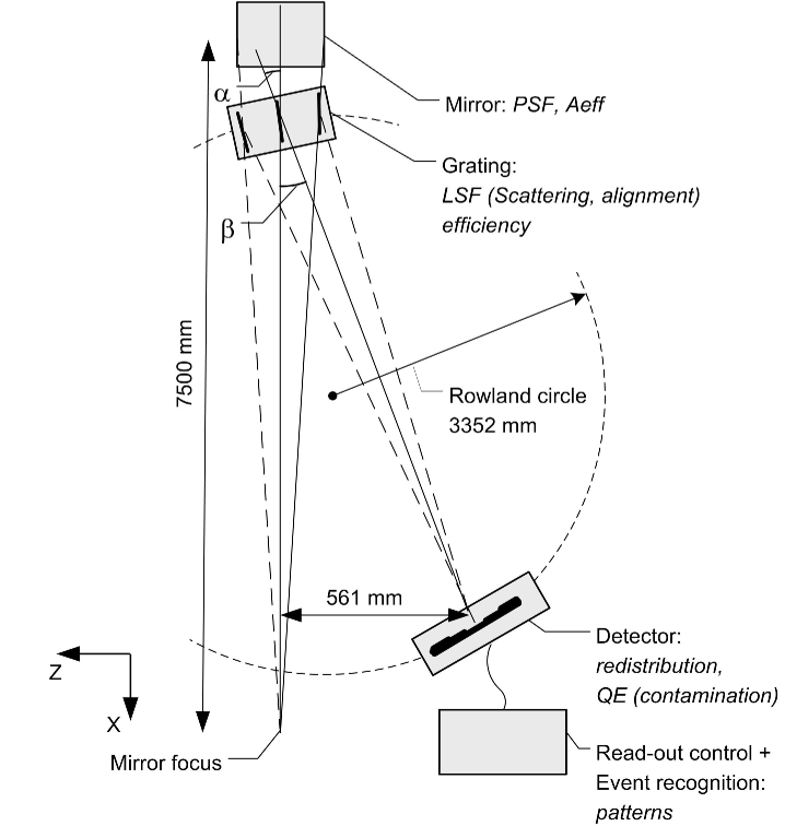
Figure 1: Schematics of the RGS configuration (not to scale)

The central position of the X-rays on the detector is given by the dispersion equation through:

$$m\lambda=d\leavevmode\nobreak\ (\cos\leavevmode\nobreak\ \beta\leavevmode\nobreak\ -\leavevmode\nobreak\ \cos\leavevmode\nobreak\ \alpha)$$ (1)

where $m$ is the spectral order (–1, –2), $d$ is the groove spacing, and $\alpha$ and $\beta$ are the angles of the incident and dispersed rays measured from the grating plane. First and second order spectra are overlapping on the detectors and using the energy resolution of the detector they can be easily separated. For extended sources the wavelength resolution degrades to

$$\Delta\lambda=0.124\leavevmode\nobreak\ \times\leavevmode\nobreak\ \theta\leavevmode\nobreak\ /\leavevmode\nobreak\ m$$ (2)

where $\theta$ is the source extent in arc min and $\Delta\lambda$ in Å. The instrument is optimized at 15 Å around the Fe-L lines. Key parameters of the design are listed in Table 1.

Table 1: Key design parameters

parameter value comment $\lambda\rm_{blaze}$ 15 Å first order blaze wavelength $\delta$ 0.6989^∘ blaze angle of facets $\gamma$ 2.2751^∘ graze angle on facets $\alpha$ 1.5762^∘ angle of incidence $\beta\rm_{blaze}$ 2.9739^∘ diffraction angle for $\lambda_{\rm blaze}$ $1/d$ 645.6 lines/mm central groove density CCDs 9 back illuminated, $\sim 30\mu$m thick pixels 27 $\times$ 27 $\mu$m² pixel size; standard $3\times 3$ on chip binning CCD size 1024 $\times$ 384 image area, identical storage area T $-80$ to  -110$\,{}^{\circ}{\rm C}$ $\lambda$-range 6.0 - 38 Å $A_{\rm eff}$ $140\leavevmode\nobreak\ {\rm cm}^{2}$ for two units at 15 Å resolving power 100 - 500 $\approx 250$ at 15 Å $\Delta\lambda$ 8 mÅ wavelength accuracy

Each instrument consists of four different units: the reflection grating assembly (RGA) which is an assembly of accurately positioned gratings; the RGS focal plane camera (RFC) which is an array of 9 CCDs in which the reflected photons are detected; the RGS analog electronics (AE) which contains part of the data processing chain and controls the read-out sequence of the CCDs and the RGS digital electronics (DE) which controls the instrument and performs event pattern recognition.

Reflection gratings (RGA): 182/181 in-plane reflection gratings for RGS1/2 are accurately placed in the exit beam of the X-ray telescopes. Each grating is 200 mm long by 100 mm wide with a gold reflecting surface and a ruggedized backside with 5 supporting ribs to control the surface errors. Each grating is mounted at its four corners. To correct for the beam convergence, the line density of the gratings varies with position $x$ on the grating in such a way that line density is 645.6 lines/mm at grating center, while being 665.3 lines/mm at $x=+100$ mm and 626.8 lines/mm at $x=-100$ mm. The gratings are mounted in a Rowland circle configuration, on a support structure made of Be because of its mass and low thermal expansion coefficient. To maintain the proper focusing of all gratings the temperature gradient over the grating assembly should be less than 1^∘C.

The X-rays are recorded by an array of 9 CCDs in the RGS focal plane camera (RFC). This camera is passively cooled to reduce the dark current to an acceptable level ($\leq 0.06\leavevmode\nobreak\ {\rm e}^{-}{\rm/pixel/s}$). To have a good QE ($\geq$ 80%) at low energies, the CCDs are illuminated from the backside, avoiding the absorption that would otherwise be caused by the gate structure at the front side of the CCDs. To reduce the sensitivity for optical load, the CCDs are coated with a thin aluminum layer with a thickness of 45 nm, 60 nm and 70 nm depending on the relative position of the CCD with respect to the mirror focus. To isolate the Al layer from the CCD itself an insulating ${\rm MgF}_{2}$ layer has been applied. These components produce absorption edges in the response of the instrument. Subsequently the X-rays are absorbed in the high-epitaxial Si ($\geq 10\leavevmode\nobreak\ \Omega{\rm m}$) (jansen1989). For each absorbed photon the number of electrons is proportional to the energy of the incoming photon. To avoid unnecessary diffusion of the produced electron cloud in the Si prior to charge cloud collection and read out near the gate structure, the CCDs are thin ($30\mu m$). This implies that the QE around the Si-edge is less than 100 %. In addition, some charge will be lost for events absorbed near the backside of the CCDs. This causes a partial event tail in the CCD redistribution function.

All CCDs have an image and a storage section and are read out in frame transfer mode. The clock pattern for this read-out is programmable and it is possible to perform on-chip binning, to read out only parts of the CCD, or to read out the full CCD through one or both of its two output nodes. During standard operations the charge of $3\times 3$ physical CCD pixels of $27\mu{\rm m}\leavevmode\nobreak\ \times\leavevmode\nobreak\ 27\mu{\rm m}$ is added on the CCD (these $3\times 3$ pixels are referred to as a bin). Still, the charge generated by a single X-ray event can be split over more than one bin causing so-called split events. To ensure the direct relation between charge and photon energy, pile-up (two events in the same bin or in neighboring bins during a read-out) should be avoided. The typical read-out time per CCD, with the two CCD halves read out simultaneously through both output nodes, is $\approx 0.6$ s, resulting in a readout time of 4.6 s for the array of 8 operational CCDs. Except for very bright sources such as e.g. Sco X-1 or the Crab the pile-up is very small (normally well below 1-2 %).

In addition to X-rays dispersed by the gratings, the cameras also register X-rays from four onboard calibration sources located in the thermal/radiation shield just around the detector. $\alpha$ particles from a Cm244 source illuminate an Al target generating Al-K line emission in two sources. For the two other sources a Teflon target has been selected, generating F-K$\alpha$ emission. The generated X-rays do not overlap with the image of a point source and their energies do not interfere with the 1st and 2nd order dispersed source spectrum.

The analog electronics (AE) controls and selects the CCD to be processed and measures the amount of charge in the output node of the CCD. It amplifies the signal and adds an electronic offset, before passing the signal to the ADC of the digital electronics.

The digital electronics (DE) processes the data. Bins with only the dark current and electronic noise (lower threshold) and bins with a too high charge due to a charged particle hitting the detector (upper threshold) are immediately rejected. The remaining bins are searched for acceptable event patterns (combination of adjacent bins within a $2\times 2$ bin region which are characteristic for a true X-ray event). Patterns larger than a $2\times 2$ bin region are rejected. The DE also stores a list of uploaded hot pixels and columns, used for rejection of these items. The relative loss of CCD area due to interactions of charged particles is computed for each CCD readout frame. Later, on ground, the effective exposure time for each CCD readout frame is corrected in correspondence with this relative loss of CCD area and for the known hot pixels and columns.

In addition to this routine data processing, full frames are stored at a very low rate of one every 15 minutes and using spare telemetry capacity these full frames are transferred to ground. This provides diagnostic data to monitor the CCD performance in full detail. A cold redundant digital electronic unit is present.

The main observable parameters are the position along the dispersion axis (the photon wavelength), the position in the cross dispersion direction and the photon energy as recorded by the pulse-height in the detector (for order separation). In Fig. 2 these data are shown for a point source. In addition to the X-rays from the celestial source, the four on-board calibration sources with different energies (F-K_α at 0.677 keV and Al-K_α at 1.487 keV) are clearly visible.

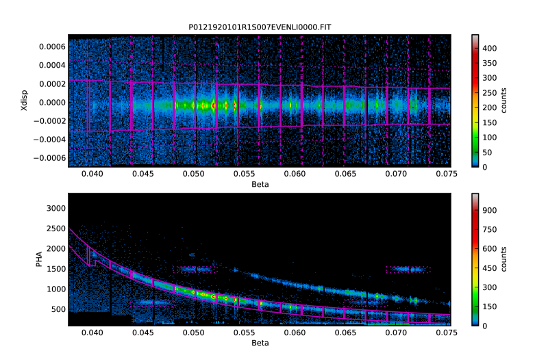
Figure 2: Capella observation (id: 0121500201001). The color scale represents a logarithmic intensity scale. The dispersion (Beta) axis runs horizontally and increases to the right. All angles (Beta, Xdisp) are in radians. In the top panel the cross dispersion (Xdisp) is along the vertical axis whereas in the bottom panel this is replaced by the CCD recorded photon energy, or PHA, in units of eV. In the bottom panel the low level thresholds are clearly visible. Standard data selections for first order are indicated by the solid purple curves.

3 Calibration basics

3.1 Calibration elements

The response of an instrument describes the conversion from photons incident on the instrument to the data actually recorded by the instrument. For a spectroscopic instrument like RGS the response key elements are effective area, wavelength scale, and linespread function. We define these elements as follows:

Effective area: This quantity is a function of energy ($A_{\rm eff}(E)$), and is defined as the ratio between the observed source count rate (${\rm counts\,s}^{-1}$) and the incident photon flux (${\rm photons\,s}^{-1}{\rm cm}^{-2}$) For RGS the effective area can be decomposed into the product of the following different components:

• Mirror area $\times$ mirror efficiency

• Grating efficiency

• CCD quantum efficiency

• Exposure fraction

• Data selections

The different components depend on a multitude of parameters. The mirror geometrical area is the front surface area of the total instrument. The CCD quantum efficiency (QE) includes all losses in the absorbing and dead layers on the CCD, charge transfer efficiency (CTE), onboard signal thresholds and processing etc., and depends on the actual CCD chip and location on the chip. The exposure fraction is relative to the real observing time. Apart from dead times caused by onboard processing limitations and cosmic ray hits it also includes the effects of instrument pointing variations. These variations move photons to different pixels on chip locations with different QE or dead pixels. Subsequent data selections also affect the number of recorded photons.

Linespread function (LSF): This is the probability distribution of the location where photons of given energy land on the detector, ${\rm LSF}(E,pointing,..)$. This depends on the quality and internal alignment of the optics, both in terms of optical surface accuracy and scattering contamination. Pointing reconstruction accuracy and data selections also contribute.

Wavelength scale: This function is defined as the relation between the energy of the incoming photon and the most likely location, which is the center of the linespread function, where it will end up on the detector, $W(E)$. This depends on pointing, grating parameters and the internal alignment of the different instrument components.

Table 2 gives an overview of the different dependencies. In the next sections these components are treated in more detail.

All response elements may change over time, but during the operational period a few major adjustments caused sudden changes to specific components. Further cooling of the detector, change of CCD readout mode and adjustment of CCD bias voltage had major impact on the response. Details of these instrumental operations are described in section 11 and listed in table 12.

Table 2: Calibration dependency

parameter	dependency
line spread function	mirror PSF
	gratings alignment
	gratings scattering
	particle contamination of the optics
	(causes additional scattering)
	pointing reconstruction accuracy
wavelength scale	grating dispersion parameters
	mirror – grating assembly alignment
	focal plane camera position
	CCD positions in the camera
	stability of optical bench
	pointing reconstruction accuracy
effective area	mirror effective area
	geometrical overlap gratings/mirrors
	grating efficiency
	CCD quantum efficiency
	CCD molecular contamination
	CCD ’absorption’ layers (filters)
	CCD thickness
	event pattern processing
	CCD redistribution
	read-out noise
	CCD dark current
	charge transfer inefficiency
	X-ray event pattern
	exposure
	satellite pointing
	CCD cosmetic defects
	particle background
	data selections

3.2 Calibration method

Accurate calibration is a long and tedious process. As a full mapping of the response over all energies and all source positions is impossible, we combine models, constrained or verified by real measurements. Subsequently this model was updated using in-orbit data.

The calibration starts with the physical understanding and measurement of the response for different units including the mirror, the detector (first as CCD, subsequently as integrated camera) and the reflection grating assembly (first as grating plate, later as integrated RGA).

Following the detailed calibration of the physical models, the instrument response is compared with end-to-end performance tests at the MPE Panter facility (Freyberg2005; Brauninger2004) at specific energies and positions in the field of view. The major limitations of this approach are:

• the measurements can be performed only for a limited number of energies and angles;

• no X-ray sources with narrow emission lines below $\sim 1$ keV exist;

• due to the finite source distance the first part of the mirror is not fully illuminated resulting in a not fully representative measured mirror response;

• the alignment of the units cannot be tested on the ground as the correction for the finite source position (120 m) requires a different relative alignment of the units than in orbit.

To cope with these limitations for the ground calibration a dedicated calibration campaign in the first months in orbit was foreseen. With a number of astrophysical sources unknown calibration parameters, such as the wavelength scale, could be fixed.

Following this early phase in-orbit calibration a set of ’routine’ calibrations are performed with different aims:

• Effective area stability: The stability of the effective area is checked by bi-annual measurements of two stable soft sources: the isolated neutron star RXJ1856-3754 and the Vela Pulsar Wind Nebula. Two other sources turned out to be less suited: the isolated neutron star RX J0720.4-3125 showed to be variable (devries2004), and SNR 1E0102.2-7219 (or N132D) is an extended source. In extended sources, spatial and spectral information is mixed, which means that if the source is not circularly symmetric, the extracted spectrum depends on the roll angle of the satellite, and is therefore less suitable for a regular verification of the effective area. Measurements of a strong continuum source (BL Lacs PKS 2155-304 and Mrk 421) allow a check on the stability of the oxygen edge, which can change over the mission lifetime due to the accumulation of ice on the cooled detector.

• Wavelength scale: Initially a set of coronal sources were measured regularly. AB Dor once a year, Capella and HR 1099 alternating also once a year. Recently this has been reduced to Capella once a year only because the wavelength scale does not show long term trends.

• CCD response: Dedicated measurements with Mrk 421 on and off-axis allows the measurement of the CTI in the detectors. For different positions off-axis in the cross-dispersion direction, the number of parallel transfers in the CCD varies, and this allows an accurate calibration of the parallel CTI. The sides of two adjacent CCDs are read out in opposite direction. For RGS2, after revolution 1408, all pixels are read out trough one single node. Due to these serial transfers the pixels near the CCD edges are hardly affected whereas the pixels in the center, with typically 512 or 1024 transfers, show a reduction of a few percent in pulse height. This is observed as a saw tooth shape of the recorded CCD pulse heights versus dispersion direction in the spectrum, that disappears after calibrating the serial CTI.

  In addition, the observations of Capella are used to verify the CCD electronic readout gain, defined as the conversion factor from captured electric charge to pulse height readout units, and the serial CTI calibration of the CCDs.

  Furthermore, full frame CCD images, obtained during all observations, allow us to monitor the development of artifacts due to radiation damage in the CCDs and the changes in the read-out noise and dark current of the CCDs.

• Non-routine calibrations: In addition, non-routine calibrations are carried out to investigate certain aspects. A detailed measurement of the Crab spectrum was carried out with the aim of calibrating the absolute effective area (Kaastra2009) and of Sco X-1 with the aim to fully characterize the X-ray absorption edge structures present in the CCDs response (devries2003).

Some of these measurements were planned to coincide with the same target in the Chandra observatory observation program. Detailed comparison of our results with those of Chandra is, however, outside the scope of the current paper. Information on cross calibrations between high energy missions can e.g. be found in the proceedings of the IACHEC meetings (http://web.mit.edu/iachec/)

Table 3: Current inflight calibration plan

purpose	frequency (/year)	measurement
$\lambda$ calibration	1	coronal source: Capella
effective area	2	continuum source: Mrk 421, PKS 2155-304 1
	1	Vela SNR
	1	RXJ 1856–3754
CCD response (gain/CTI)	0.5	Mrk 421 on and off axis (CTI) 1
	1	Capella (gain)

• During the period when Mrk 421 is not visible, it is replaced by PKS 2155-304

3.3 Calibration files

The basic tool to analyze RGS spectra is the instrument response matrix (RSP). The response matrix is the product of the mono-energetic X-ray redistribution (RMF), the effective area (ARF) and exposure map. Data channels are re-binned CCD columns in the dispersion axis ($\beta$-angle) or in wavelength ($\lambda$) space. The exposure map contains for each data channel the relative exposure time of that channel with respect to the exposure time of the observation. E.g. discarded bad CCD pixels or columns in the instrument, CCD dead times due to lost telemetry packets are accounted for in the exposure map. In the total response matrix, all these different elements of the calibration are combined.

Over time the understanding of the instrument response will evolve, both in terms of additional or improved calibration data, and in terms of improved instrument models. In addition, the calibration of the instrument is not static but varies over time. This is accommodated by the current calibration files (CCF). These CCFs store the parametrized instrument response and are used by the instrument model. The CCFs are tagged with a time validity interval, usually spanning many observations, which allows to have parameters which slowly change with time (gain, CTI, bad pixels). Changes can be accommodated by updating the relevant CCF. Only occasionally the actual data processing code needs to be updated to accommodate improvements in instrument models. The relevant CCFs are given in Table  4. The actual CCFs, including their sequence number and validity start time are given in Table 14. The CCFs were designed with flexibility in mind; some CCFs contain elements which later turn out not to be used.

Main steps in the RGS data calibration processing are as follows:

• Event processing. From each recorded event, the CCD noise level is subtracted on a pixel by pixel basis, as derived from a three orbit average computed from CCD images, and the recorded pulse level (PHA) is converted to eV using the gain and CTI calibration. Warm/hot pixels are detected, and corresponding events discarded.

• Wavelength. Using the spacecraft pointing information and instrument geometry, the conversion from detector coordinates to $\beta$/wavelength space is computed.

• Spectra. Using the given spatial, PHA, and time selections within the observation, source and background spectra are computed in detector channel (either $\lambda$ or $\beta$ space).

• Response. Using the appropriate calibrations for the time of observation, the response matrix is computed.

Instrumental background is usually obtained from off-source regions in cross dispersion on the detectors, using identical PHA selections as for the source. This works very well for sources which illuminate only a fraction of the RGS cross-dispersion field of view (4.9 arcminutes), but cannot be used for extended sources which cover the entire detector. For this reason a separate set of calibration files is maintained which provide backgrounds derived from empty fields. These backgrounds are mainly generated by the fluctuating soft proton flux and cover a variety of different flux levels. The background in this case is constructed by selecting the appropriate background calibration files, based on the soft proton level indicators constructed from CCD9 count rates (see also section 10.1).

Table 4: CCF files, applicable to RGS

CCF	contents
ADUConv	gain (ADC to eV conversion)
	average noise level (not used)
CTI	parallel and serial CTI correction
BadPix	bad pixels, segments and columns
	h = uploaded, H = on ground only
CoolPix	additional hot/cool pixels
Quantum Efficiency	CCD filter layers and Si thickness
	RGA efficiencies and vignetting1
EXAFS	${\rm MgF}_{2}$ edge and O edge
EffAreaCor	contamination correction
	correction for large scale variation
ReDist	CCD PHA redistribution parameters
LineSpreadFunc	RGA figure/alignment errors and scattering parameters
CrossPSF	source profile in cross dispersion
LinCoord	relevant alignment parameters affecting wavelength scale
TemplateBackground	spectra for pre-defined background
	intensities for data selections
XRT XAreaEff	mirror effective area and vignetting2
XRT XPSF	mirror RGS point source PSF profile, used for LSF computation
XMM BoreSight	instrument alignment parameters
MiscData	various additional parameters
HKParmInt	RGS housekeeping parameter limits
SAACorr	coefficients for the sun angle wavelength correction
ClockPatterns	CCD clock pattern parameters
XMM ABSCoef	Henke absorption coefficients for certain elements

1) The geometrical effect that for photons leaving a grating at larger angles the backside of the neighbouring grating may block part of the X-rays (shadow effect). This depends on spacecraft pointing and energy of the photons.

2) The geometrical effect that for off-axis angles, the mirror shells may partially block each other. Blocking is different for different parts of the mirror, which means there will be some energy dependence, since reflection efficiency differs depending on photon energy and reflection angle.

4 Mirror calibration

The two main functions describing the mirror response are (a) the Point Spread Function and (b) the effective area. Of course they depend on the offset from the optical axis. In Fig. 3 we show the measured mirror PSF, projected on the RGS dispersion axis, and the mirror model used for RGS. The model consists of a combination of a Gaussian and a Lorentzian function, which are parametrized in the CCF.

Although systematic effects dominate there is a good match, in general within 2–4 $\sigma$ for the wings, between the model and the data with the exception of an overprediction towards the core of the distribution. This can be explained by some pile-up in the core of the measured distribution. However, the angular scale of this mismatch is small compared to the RGS LSF, so this hardly affects the modeled LSF.

The total RGS LSF width ($\approx 30$ arc seconds FWHM) combines the mirror PSF ($\approx 6$ arc seconds FWHM) and the grating scattering and internal misalignment’s. RGA scattering is the most dominant factor (see Fig. 28).

Figure 3: Measured and modeled mirror response (projected on the dispersion axis). Fit residues (lower plot) are given in units of the statistical error.

5 Detector calibration

Due to radiation damage, the detector properties change over time.

The CCD response is only used to separate orders and has only an indirect effect on the spectral resolution for a grating spectrometer. Its main impact is the data selections in CCD pulse height that affect the instrument effective area.

5.1 Detector model

We developed a model for the detector response based on a simplified and phenomenological approximation of the interaction of a photon and the detector. Fig. 4 shows a crosscut through an RGS back illuminated CCD. The probability $P$ for absorption of the X-ray photon at penetration depth $x$ is:

$$\frac{{\rm d}P}{{\rm d}x}=\frac{1}{\tau}\cdot e^{-x/\tau}$$ (3)

with $\tau(E)$ the absorption depth for silicon for X-ray photon energy $E$ as derived from Henke.

At the spot of the X-ray photon absorption, an amount of electric charge is released proportional to the incident energy of the photon. We define the electric charge in units of the energy of the X-ray photon. This scale of course implies the calibration of the electronic signal.

Not all charge released will make it to the output node of the CCD. The collected charge $Q$ from the X-ray event depends on the depth at which the charge is generated. The deeper the penetration, the closer to the front side structure and the more of the generated charge is collected. This is modeled by:

$$Q=\left\{\begin{array}[]{ll}0&{\rm for\leavevmode\nobreak\ }E<T\\ T+(E-T)\cdot(1-e^{-{(x/b)}^{1/3}})&{\rm for\leavevmode\nobreak\ }E\geq T\\ \end{array}\right.$$ (4)

with $T$ the threshold for charge detection and $b$ a scale parameter. These parameters were derived from ground calibrations and set at $T=50$ eV and $b=20.95$ nm.

The charge probability density can be written as:

$$\frac{{\rm d}P}{{\rm d}Q}=\frac{{\rm d}P}{{\rm d}x}\cdot\frac{{\rm d}x}{{\rm d}Q}$$ (5)

From (4) we derive:

$${\rm d}Q=(E-T)\cdot e^{{-(x/b)}^{1/3}}\cdot{\left(\frac{x}{b}\right)}^{-2/3}\cdot\frac{1}{3b}{\rm d}x$$ (6)

and:

$$\frac{{\rm d}P}{{\rm d}Q}=\frac{1}{\tau}\cdot e^{-x/\tau}\cdot\frac{3b}{E-T}\cdot e^{{(x/b)}^{1/3}}\cdot{\left(\frac{x}{b}\right)}^{2/3}$$ (7)

From 4 it follows:

$${\left(\frac{x}{b}\right)^{1/3}}={\rm ln}\frac{E-T}{E-Q}$$ (8)

which allows to eliminate $x$ from (7):

$$\frac{{\rm d}P}{{\rm d}Q}=\frac{3b}{\tau}\cdot\frac{1}{E-Q}\cdot{\rm ln}^{2}\left(\frac{E-T}{E-Q}\right)\cdot e^{-\frac{b}{\tau}{\rm ln}^{3}\left(\frac{E-T}{E-Q}\right)}$$ (9)

To this function (9) a constant partial event floor $t$ is added that has constant probability density below the incident energy and is zero above. The resulting redistribution function $\frac{{\rm d}R}{{\rm d}Q}$ thus becomes:

$$\frac{{\rm d}R}{{\rm d}Q}=\left\{\begin{array}[]{ll}\frac{{\rm d}P}{{\rm d}Q}&{\rm for}\leavevmode\nobreak\ Q\geq E\\ \frac{{\rm d}P}{{\rm d}Q}+t&{\rm for}\leavevmode\nobreak\ Q<E\end{array}\right.$$ (10)

The partial event floor $t$ is normalized to the total partial event fraction $P_{\rm part}$:

$$P_{\rm part}=\int_{0}^{E}t\>{\rm d}Q=t\cdot E$$ (11)

$P_{\rm part}$ is 0.0348 for $E=1.9$ keV and scales with $(1-e^{-1.832\cdot E})\times\tau(1.9{\rm keV})/\tau(E)$ with $E$ expressed in keV.

Finally, this shape is convolved with a Gaussian with a width of $\sigma$ to account for the fano (Fano) and amplifier noise:

$$\sigma=\sqrt{(a\cdot\sqrt{s}\cdot w)^{2}+wfE}$$ (12)

with $a=5.4$ the amplifier noise, $w=3.65$ the electron creation energy, $f=0.14$ the Fano noise factor and $s$ a scale factor, depending on the OCB pixel size with $s=1.4$ for 3x3 OCB and $s=2.5$ for 1x1 OCB.

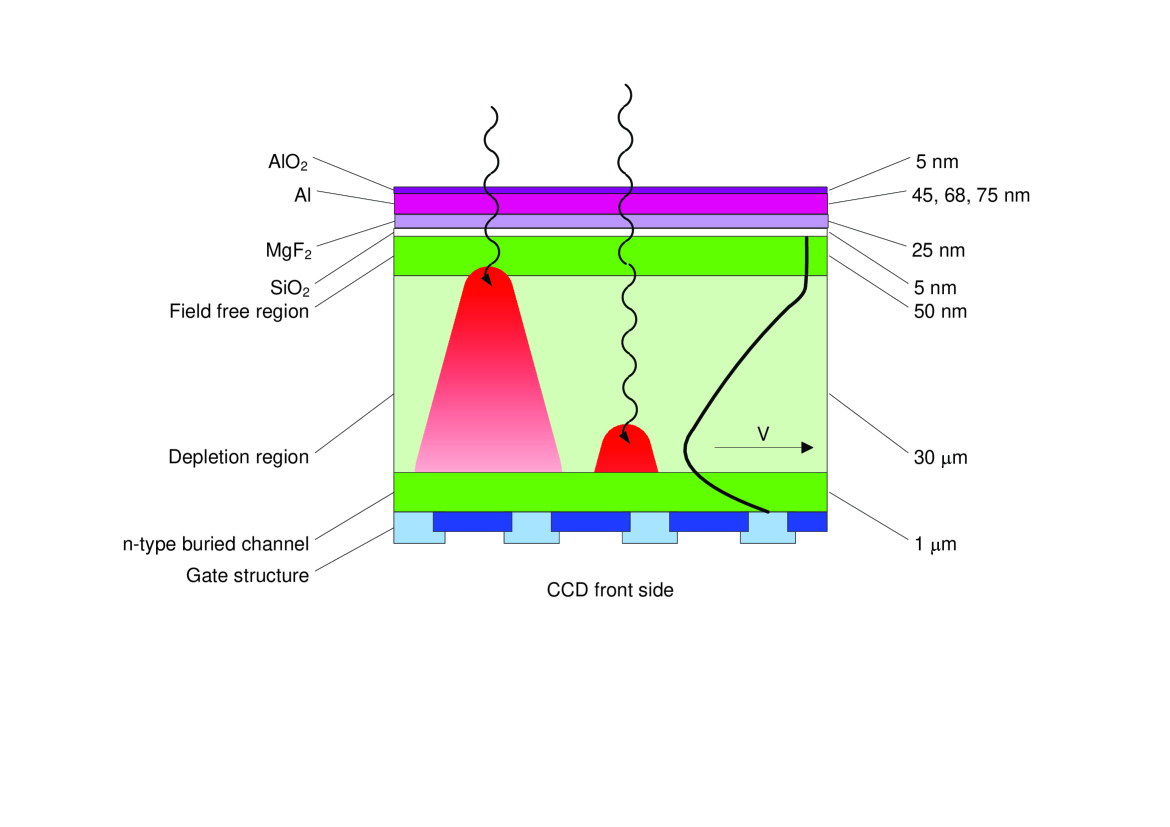
Figure 4: Model of the CCD indicating all different layers. X-rays entering from the top will be absorbed at a certain depth. An X-ray photon of low energy might be absorbed close to the field free region, losing part of its charge; higher energy X-rays will be absorbed closer to the gate structure and therefore the charge diffusion in the depleted region will be smaller (indicated by the flat mountain shaped area in the figure). At the right the potential in the CCD is indicated.

Fig. 6 shows the different components in the final model function. This CCD redistribution function is checked in flight at regular intervals to see whether the CCD charge collection is stable using bright mono-energetic emission lines of our wavelength calibration sources (notably Capella) (Figs. 7 and 8). The incomplete charge collection of charge created near the back side (see Fig. 4) which mainly affects low energy X-rays, or X-rays just above the Si edge, causes the tail of the function to lower energies. This strongly asymmetric function with its tail towards low energies, combined with the convolution by a symmetric Gaussian for the Fano and amplifier noise, causes the peak of the function to be shifted towards lower energies, as schematically shown in Fig 5, to below the original incident X-ray energy. The effect is less at higher energies. In both figures 7 and 8 the effect of leakage of the second order events is shown. Also clearly visible is the improved resolution at higher energies and the tail of the noise floor at lower energies.

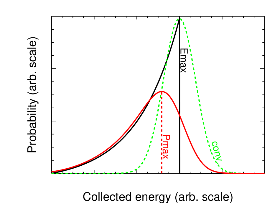
Figure 5: Schematic view of the effect of convolving the strongly asymmetric collected charge probability (solid black curve) for a photon with energy $E{\rm max}$ with a symmetric Gaussian shape (broken green line) of the noise distribution. The resulting probability distribution (red curve) will have its maximum $P{\rm max}$ shifted to lower energy than the original photon energy $E{\rm max}$.

This redistribution function can be regarded as the response to mono-energetic incident X-rays, in which the peak of the collected energy does not necessarily coincide with the initially absorbed energy. Using such a distribution enables calibrating a simple linear gain relation between collected charge and CCD electronic output. When the observed peak of the redistribution function would be used to define the CCD energy scale, a highly non-linear function would be needed.

Figure 6: Model of the CCD response, or charge collection efficiency (CCE), which is the probability for the collected energy, illustrating the key components. Also shown is the 95 % window which is the default data selection (vertical lines). For completeness we also show the typical read-out noise (system) which gives the typical output for a pixel without absorbed X-ray. The electronic bias level of the CCD has been subtracted from the energy axis, causing the read-out noise system peak to extend below the zero energy level.

Figure 7: Modeled and observed CCD response for the N vii ${\rm Ly}\alpha$  line (24.779 Å= 500 eV). The data is a sum of 15 Capella measurements.

Figure 8: Modeled and observed CCD response for Ne X Ly-$\alpha$ line (12.132 Å= 1022 eV). The data is the sum of 15 Capella measurements.

The user can define any window for event selection. Generically the window is defined in terms of percentage of the integrated CCD redistribution function at equal cutoff levels left and right of the maximum. The default selection uses 95% of the events, identical for all energies. Fig. 6 shows this selection. This nominal window is relatively insensitive to small variations in CCD gain and uncertainty in the redistribution model. The CCD gain is calibrated at two yearly intervals by shifting the observed CCD redistribution to the model distribution. The uncertainty in the gain calibration is estimated at $\leq 1$%. The effect of the gain uncertainty on effective area is far less than 1%, since this is a second order effect.

Whereas the number of selected events, which are the actually detected photons, is largely insensitive to gain variations, the effect of the visible/UV blocking filters as well as variations in the Si thickness are clearly important. Si thickness variations over the CCDs were measured by using the interference patterns of internal reflections of infrared light (1032 nm) within the CCD chip. Due to the production process the CCDs are thinner near the edges whereas the central part of each CCD is typically flat within 2 $\mu$m. The edges can be up to 3 (one side) or up to 6 $\mu$m (other side) thinner which effects the QE at 1.8 keV of at most -4%. This effect is only relevant for those CCDs which cover the wavelength ranges between 1.5 and 1.82 keV (Si-edge) and is properly taken into account for the relevant CCDs in the calculated efficiencies.

In the model we have included absorption by the Al filter, deposited on top of the CCD with a varying thickness between 44 and 75 nm and a MgF₂ isolation layer between 23 and 29 nm located in between the Al layer and the Si (see Fig. 4), as measured by the CCD manufacturer (EEV). The uniformity of these layers was verified by UV/optical measurements at 250, 406 and 540 nm. Interpretation of these results was hampered by the lack of knowledge about the surface roughness of these layers. The effect on total absorption of possible variations in surface roughness below 24 Å is estimated to be less than 1% increasing to up to 9% at the longest wavelength ($>35$ Å).

All these factors, which also include the signal selection thresholds, are taken into account to determine the total QE of the CCD and these results were verified by ground measurements (Fig. 9). The shown model is the calculated QE based on physical (and measured) properties of the device as given in Table  5. A fair match between the measured and calculated QE is observed but, particularly at lower energies, for the C, O and F sources large deviations could easily occur. This is mostly due to the fact that at low energy the natural line width of these sources is relatively large. Attempts were made to use a separate monochromator to narrow the natural line widths of the sources, but these results turned out to be less reliable due to unpredictable and uncalibrated inhomogeneities in the monochromator beam.

Table 5: CCD parameters ranges

Al thickness CCD [nm]	44 - 75	depends on CCD position
MgF2 thickness [nm]	23 - 29	different per CCD
Event size (3x3 OCB)	1.4	binned pixels
Individual CCD total central Si thickness [$\mu$m]	26.6 - 33.4	different per CCD
Si change of thickness over single CCDs [$\mu$m]	3 - 6	decrease of thickness towards CCD edges

Figure 9: CCD quantum efficiencies, as measured during ground calibrations at Panter (herder). The symbols indicate the measured data points. Stars: X-ray atomic line energies, diamonds: monochromator data. The broken lines indicate the energies of atomic edges of the indicated atomic species. The solid line is our model.

5.2 CCD radiation hardness

Cosmic charged particles hitting the CCD detectors can damage the CCD. Either the Si depletion region is damaged, giving rise to local low resistivity causing high dark current and hot pixels, or the charge transfer layer at the front side (opposite the back side where the X-ray photons enter) is hit, which may cause an increase in charge transfer inefficiency (CTI). Increased CTI will cause a drop in the PHA pulse height and a decrease in the CCD energy resolution. When CTI becomes too high, $1^{\rm st}$ and $2^{\rm nd}$ orders cannot be separated any more and the dispersed spectrum will become indiscernible from the system peak.

A set of protection measures have been implemented. By applying proper shielding around the detector, 3 cm Al coated with a Au layer, only particles with high energies, mostly protons, will reach the detector directly in addition to the secondary radiation from these particles in the shielding. Also the design of the CCDs and their operations reduce the effect of radiation damage. Buried channels in the CCDs confine the charge to a limited volume, reducing the relative size of the damage with respect to the signal. An operational temperature range can be selected for which the dark current and cosmetic blemishes can be reduced. Together these measures allow to handle the expected dose of $10^{9}$ 10 MeV equivalent protons and  1 krad (after applying the 3 cm shield), which is representative for the expected dose over a mission of 10 year (jansen1989).

However, Chandra experienced an unexpected damage of their CCDs during the first part of the mission (prigozhin2000; dell2000). This could be attributed to soft protons focused by the X-ray mirrors onto the detectors, encountered during the passage through the radiation belts. To quantify this effect for our detector, flight representative RGS CCDs were subjected to protons at various low energies in the Van der Graaff accelerator in Utrecht. Table 6 presents the results for one representative CCD illuminated from the CCD backside, which is the same side as illuminated in orbit. The device was about 24 $\mu$m thick although there is a significant variation over the CCD. We selected 6 different energies with a stopping range from 10 $\mu$m to 30 $\mu$m. At low energies the protons are stopped in the bulk material whereas at the higher energies the protons are stopped in the layer where the charge is transferred. At the highest energies the majority of the protons are stopped by the gate structure, or pass the CCD without causing serious damage.

Table 6: Sensitivity of RGS CCDs for soft protons normalized to a fluence of $5\leavevmode\nobreak\ 10^{7}$ protons per cm² (stopping ranges from SRIM: http://www.SRIM.org).

$E_{\rm proton}$	stopping range	CTI/transfer	${\rm{I_{dark}}}$
MeV	$\mu$m	[$10^{-5}$]	ratio (post/pre)
0.75	10.9	3.4	6
1.15	20.5	7.8	2
1.27	23.8	95.7	5
1.40	27.7	306.6	46
1.45	29.2	61.6	n/a
1.55	32.4	18.0	n/a

In Fig. 10 the change in CTI is given for different radiation levels and different proton energies. Although it was planned to test each energy up to a fluence of $10^{8}$ protons/cm² at the lower energies the beam was about a factor of two more focused than anticipated. This explains the differences in the maximum fluences. As can be seen the CTI degrades most between 1.27 and 1.40 MeV, corresponding to a stopping range between 24 and 32 $\mu$m, which is in fair agreement with the thickness and uniformity of the CCD. In addition, we observed that the charge transfer efficiency improves considerably if the CCD is stored at a higher temperature for one night following the irradiation by the protons. This is a known effect in CCDs. In Fig. 11 we provide the integrated CTI (over typically 200 transfers) for 4 different energies at their maximum fluence. As is also known from higher energy protons, the largest CTI occurs between -80 and -100 ^∘C. At higher temperatures the CTI improves artificially; due to the high dark current the traps are filled for a large fraction of the time. However, under this condition it is hard to impossible to separate the real events from the dark current. Cooling the CCDs below -100 ^∘C improves the CTI considerably because the release time of charge from the traps becomes longer and thus their impact on the CTI will be less (they are filled for an increasing part of the time). The curves in Fig. 11 are for a different total dose. No data were measured to correct for this at other temperatures than -80 ^∘C. Finally we list in Table 6 the increase in the dark current. This also peaks at 1.40 MeV which is consistent with stopping of the protons around the interface between the bulk Silicon and the gate structure.

Based on these results, the energy dependence of the proton scattering from the mirror and gratings (section 6.4), and the spectral shape for soft protons ($E^{-1.7}$), the RGS CCDs were expected to be hardly affected by soft protons. This has indeed been confirmed, although it is impossible to separate soft and hard protons using flight data only. The absence of a filter wheel has not caused any unexpected problems. To identify a time period of high proton flux the RGS detector closest to the optical axis (CCD9) is monitored and if the count rate for a part of the CCD not corresponding to the source image increases above a set level, the EPIC filter wheel will be moved to its closed position.

Figure 10: CTI as a function of the fluence for different energies of the protons. Curves are fit to the data.

Figure 11: CTI as reflected in the PHA position of the Al-K line as function of temperature and radiation dose.

5.3 Read-out noise and dark current

In Fig. 12 we show the typical response of a single detector bin when exposed to X-rays. Most of the time no X-rays are observed, and the detected charge is a measure for the electronic noise and dark current. When an X-ray is absorbed in a bin the corresponding charge increases (the spikes in the figure). The data free from X-ray events are called the noise floor or system peak in the RGS specific descriptions.

The noise floor level is formed by the integrated dark current, on top of the electronic offset. Due to radiation damage and operational conditions, dark current and consequently the noise floor gradually changes over the mission lifetime (Fig.  13). Major changes in the operational conditions are indicated. Clearly the increase due to a strong solar flare (orbit 110), the change due to the CCD bias tuning (orbit 168), the reduction in dark current due to lowering the operational temperature (orbit 532 and 537), and the increase in dark current following the change to a single node read-out which resulted in longer integration times, in RGS2 (orbit 1408), are visible. From the change in noise floor between the two node read-out and the single node read-out corresponding to a change of about a factor 2 in read-out time, the dark current could be determined as 0.14 e^-/bin/s where a bin is 0.00656 mm².

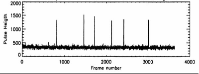
Figure 12: Response of a single detector pixel to X-rays

Figure 13: Evolution of system peak for one node of CCD5 in RGS1 and in RGS2 (other CCDs show a similar behavior). The sudden increase of the peak around orbit 110 (most prominent in RGS1) is due to a solar flare, while the drop around orbit 168 (also indicated for RGS1) is due to the change in bias setting. Cooling lowers the system peak around orbit 532, while the single node readout in orbit 1408 increases the RGS2 system peak.

In addition, we observe a small ($\Delta$ ADC $\leq$ 30 ADU) systematic pattern in the maps of the noise floors in the CCDs (Fig. 14). Following the change to the single node read-out this pattern disappeared in RGS2, clearly indicating that this pattern is caused by cross talk between the two read-out chains. Although the effect is small compared to the energy resolution of the detectors ($\geq 100$ ADU), and affects only $\approx 1$% of all pixels it can, in principle, be corrected if the pattern is known. Unfortunately this noise pattern is not fixed and drifts slowly over time and is not correlated with any of the instrument operational steps (e.g. there is no synchronization with the start of the read-out of a CCD).

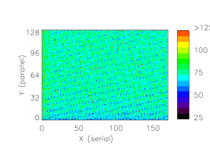
Figure 14: Fixed pattern noise (RGS2:CCD1_C, two-node readout)

Following orbit 786 RGS1 CCD1 developed two hot spots (Fig.  15). The origin of these spots is not clear as it shows up symmetrically in one CCD only. If it is radiation damage or a change in stress in the Si due to aging of the gluing to the detector bench, one does not expect it to be symmetric for the two read-out nodes. It is possibly related to flat-band voltage shifts of the CCD due to radiation damage but this can not be verified. Fortunately this feature is limited to this single CCD only and its area does not increase over time. The onboard software excludes these areas from processing.

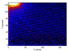
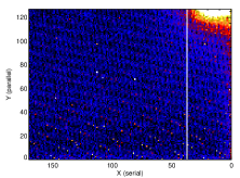
Figure 15: Hot spots on RGS1 CCD1 with separate images of nodes C and D. The hot spot intensity is about 180 ADC units above the system level floor of about 100 ADC units.

5.4 Cosmetic defects

Local defects and damage by cosmic rays in the depleted silicon material can give rise to hot pixels and columns. Although the CCDs were selected based on the absence of hot pixels, the instrument includes some CCDs with hot pixels and hot columns (see Table 7). The presence of these cosmetic blemishes is expected to vary over the life time of the mission. Due to radiation damage new hot pixels or columns can appear, and also flickering pixels (also called random telegraph noise) can be expected. Due to the mobility of the originating charge traps some hot pixels may also disappear over the mission lifetime. This is illustrated in Fig. 16 where the charges of a few noisy bins are shown. Bins with a content below the lower threshold (e.g. only read-out noise and dark current) are rejected onboard and have a typical pulse height of 100 – 120. The variation in the patterns is huge, varying from fast damping to a somewhat bi-polar state. Following the cool down (see later) the effect of these defects in the crystal was significantly reduced.

Figure 16: Variations in temporal behavior of cosmetic defects (orbit 0440, before the cooling). The top two panels are offset by 2000 and 5000 for clarity. The small gaps in the time sequence are due to the on-board processing where patterns which are not consistent with the expectation for X-rays will be rejected to reduce the telemetry load.

Searching for these cosmetic blemishes has been fully automated and we adopted an approach to reject all potential cosmetic blemishes. The signature of bad pixels and bad columns differs from the signature of astrophysical lines which cover more pixels. Therefore we compare the frequency that a given pixel or column is above the read-out noise with its neighbors, neglecting the actual pulse height value of a given bin. If this frequency exceeds its expectations based on a binomial error propagation, the bin is rejected $(N>M+\sigma_{p}\sqrt{N(1-\frac{N}{F})+M(1-\frac{M}{F})}$ with $N$ the total number of counts in a given pixel, $M$ the minimum of the total counts in the neighbouring pixels, $F$ the total number of frames and $\sigma_{p}$ is set at 5. For the rejection of hot columns we use a similar approach.

Table 7: Hot columns and pixels (3 x 3 OCB) defined in the calibration files; suspect pixels/segments are pixels/segments which are rejected on the ground but are not persistent over the mission lifetime. The orbit is the start of the validity interval of the corresponding ’BadPix’ calibration file (see table 14)

orbit	CCD	column	segment/comment
RGS1
1	CCD1_D	38	hot column
	CCD2_C	166	hot column
	CCD3_D	93	hot column
	CCD5_D	119	hot column
	CCD7_D	77	hot segment 1-33
	CCD7_D	74	hot segment 1-33
	CCD9_D	43	hot column
	all		suspect:
			27 pixels, 5 segments,
			5 columns
276	CCD1_D	38	hot column
	CCD3_D	93	hot column
	CCD9_D	43	hot column
	all		suspect: same
536	CCD1_D	38	hot column
	CCD3_D	93	hot column
	CCD9_D	43	hot column
	all		suspect:
			5 pixels after cooling
543	CCD1_D	38	hot column
	all		suspect: 5 pixels
1110	CCD1_D	38	hot column
			suspect: 4 columns
	CCD1_C	1 - 31	suspect segment 121-128
	CCD1_D	1 - 31	suspect segment 121-128
1417	CCD1_D	38	hot column
	CCD1_C	1 - 31	hot segment 121-128
	CCD1_D	1 - 31	hot segment 121-128
	all		suspect: 4 columns
RGS2
1	CCD9_C	94	hot column
	CCD9_C	147	hot segment
	all		suspect: 1 column
			and 20 pixels
532	CCD9_C	94	hot column
	all		suspect:
			1 pixel and 1 segment
1110	CCD9_C	94	hot column
	all		suspect: 7 columns

The approach to reject cosmetic blemishes is rather conservative, but as long as it is properly taken into account in the computed exposure for each observation, it ensures that hot pixels/columns do not cause any artificial emission lines. This method translates into an exposure map with large pixel to pixel variations affecting the effective area curves (Fig. 34). In Fig. 17 we display the ’dead’ area of the two detectors over the lifetime of the mission. The step-wise increase in the early part of the mission corresponds to solar activity. Following the cool down of the detector the number of hot items reduced by a factor 5 – 10 and we expect that the total affected area will stay below 4 % over the next 10 – 15 years, depending of course on the actual solar activity in the future.

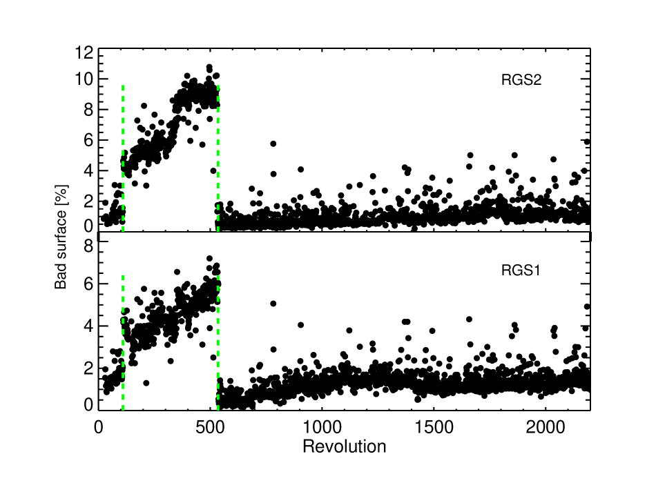
Figure 17: Bad area per detector as detected by the standard monitoring tools. The first increase corresponds to a major solar flare in orbit 110, the drop around orbit 535 is due to the cooling of the detectors from -80 ^∘C to -110 ^∘C. Individual outliers are due to peculiar observational circumstances, like e.g. periods of very high background, observations of very bright sources, or very short observations.

5.5 Warm/cool pixels

As remarked before (section 5.4), defects in the depleted region may cause local higher dark current, or extra charge traps, leading to hot and cool pixels respectively. Hot pixels are discarded, but many pixels will only show a slightly elevated dark current, which is added to the charge of recorded X-ray events, potentially shifting them outside of the pulse height selection area. Cool pixels will lower the recorded charge of events. To mitigate this effect, averages are made of CCD full frame images, recorded during three consecutive orbits around the orbit of the observation being processed. These averages are used to subtract the system peak level on a pixel by pixel bases, which will correct for the different system level peaks of hot and cool pixels.

5.6 Charge Transfer Inefficiency

Ionizing particles from cosmic rays can also cause traps in the Si lattice structure at the layer where the charge is shifted from pixel to pixel to the output node. These traps are characterized by the trapped charge relative to the total charge packet, the probability that the charge remains trapped during the charge transfer, and the probability that the charge will be emitted during the time between charge packets. Although this effect depends on the time since the last charge transfer took place through the pixel, in first approximation we can describe this by an average Charge Transfer Inefficiency (CTI) that neglects the pixel to pixel variations and pixel history. The unit of CTI is defined as the fractional loss of charge per physical charge transfer on the CCD. On the RGS CCDs there are up to 1024 transfers in the CCD X-direction, in single node readout, for the most distant pixel to reach the readout node. Our general CTI model is justified because the CCD pulse height distribution is only used to separate the orders and not for the spectral response of the instrument; our CTI correction does not need very high accuracy. The uncertainty in the total CTI correction for a pixel corresponds to 1% in the total charge for an average CTI per transfer of $10^{-5}$, to keep it the same order of magnitude as the gain error. A wider selection of the CCD response function results in a smaller error, but leads to more background. In addition to traps, the CTI is also affected by the voltages applied to the clocks when shifting charge through the CCD. Since we know the energy of the incident photons from the position on the detector, we can tune the voltages for the clocks and/or calculate the CTI corrections.

After failure of the RGS1 CCD7 readout chain CCD clock voltages were reduced to limit stresses on the components (orbit 168, table 12). These clock voltage reductions were further tuned for RGS2 CCD2 which was done in orbits 192 and 537. and the clock bias of RGS1 CCD2 needed adjustment in orbit 1389.

The Charge Transfer Inefficiency is calculated independently for the parallel transfers (transfer of the image section to the storage section or of a row in the storage section to the read-out row) and for the serial transfers (transfer through the read-out row toward the read-out amplifier).

For the parallel transfers the CTI is deduced from the measurement of a strong point source (Mrk421) at different positions in the cross dispersion direction. The difference in collected charge for different positions in the cross dispersion direction is only due to the CTI loss, as the deposited energy is given by the grating dispersion equation. This can be simply converted into a CTI calibration model.

For the serial transfers a slightly different approach is followed. CTI during readout causes the collected charge to drop depending on the number of charge shifts, given by the CCD column. Using the known energy of the photons from the dispersion relation of the grating, the relative change in charge deposited by the incoming photons over the CCD is known. The additional charge loss per transfer gives the CTI model.

The parallel and serial CTI are small (few times $10^{-5}$). Pre-launch values were around $0.9\times 10^{-5}$. Every two years special calibration measurements are executed to calibrate the CTI. Additional calibrations were performed immediately after cooling of the RGSs and following the change from double to single node readout of RGS2. Table 8 shows a moderate increase of the CTI of $10^{-5}$ over 1000 orbits but the CCD to CCD variations are larger (a few $\times 10^{-5}$. These parameters can be determined to about $0.5\times 10^{-5}$ which corresponds to an uncertainty of the energy loss of $\lessapprox 0.5\%$.

Table 8: Average CTI degradation per camera as retrieved from the calibration files (CCF) and variation (maximum difference) over all CCDs, in between brackets

RGS	orbit	serial CTI $(10^{-5})$	parallel CTI $(10^{-5})$	comment
RGS1	30	3.45 (2.90)	0.94 (0.05)	pre launch data
	260	4.16 (2.61)	4.26 (1.60)	first measurement in orbit
	536	5.05 (4.30)	4.07 (2.00)	post cooling
	807	5.07 (6.53)	6.55 (4.10)
	1397	4.89 (3.83)	7.68 (4.41)
	1839	4.96 (3.53)	8.92 (4.98)
	2021	5.92 (5.42)	11.13 (3.70)
RGS2	25	3.29 (3.14)	0.95 (0.05)	pre launch data
	260	3.55 (5.51)	3.05 (2.98)	first measurement in orbit
	532	3.87 (2.96)	2.14 (2.81)	cooling to $-115^{\circ}{\rm C}$
	536	3.48 (2.82)	2.42 (2.38)	cooling nominal
	807	3.17 (2.65)	6.11 (3.73)
	1405	2.86 (1.17)	8.06 (3.71)	to single node readout
	1839	2.71 (1.04)	9.67 (4.96)
	2021	2.58 (1.82)	11.09 (5.29)

Near the edges of the CCDs the parallel CTI is significantly larger. To reduce the dead space between adjacent CCDs in the detector array, the CCDs were sawn at the two sides, causing additional stress and hence defects in the Si. (Fig. 18). During the early part of the mission the parallel CTI near the CCD edges is $\sim 20\times 10^{-5}$, and it reduces to a few times $10^{-5}$ after the cooling of the camera in orbit 539. Over time the CTI increases again.

Figure 18: Average parallel CTI for RGS1 near the edges for different orbits. The uncertainty towards the edge increases towards about $5\times 10^{-5}$. For channels $>10$ the uncertainty is of the order of $1\times 10^{-5}$

The change in CTI was independently verified by comparing the position of the onboard calibration line positions as function of orbit. This is shown for the Al-K$\alpha$ line in Fig. 19 where the position of the Al-K onboard calibration source is shown before any gain and CTI correction. Apart from the jumps associated to CCD tuning, cooling and change to single node readout, a gradual decrease in pulse height of 3 % over the lifetime of the mission is observed. This corresponds to a change in CTI of $10\times 10^{-5}$ over 1600 orbits, consistent with the change of $5\times 10^{-5}$ in 800 orbits for the higher CCD channels, as shown in Fig. 18.

Figure 19: Change in charge transfer efficiency as reflected by the gradual decrease of the uncorrected pulse height value for events from the onboard Al-K$\alpha$ calibration sources. Major events: tuning of the CCD settings, cooling of the detector and switch to the single node read-out for RGS2, cause sudden shifts in CTI. Occasional outliers are caused by peculiar observations like e.g. bright sources, observations with high background and very short observations.

5.7 Optical sensitivity

The mirrors and gratings are near perfect reflectors for UV/optical light and this results in additional charge on the detectors for optically bright stars. The energy assigned to the X-ray photons increases by a corresponding amount and therefore is incorrectly interpreted. On the EPIC cameras this is known as ”optical loading”. The filter wheel in front of the EPIC instruments allows the user to reduce the optical light. For RGS, with its elongated focal plane, a different solution is used. For sources within the field of view the specular reflected photons are imaged on the ${\rm zero}^{\rm th}$ order position of the grating, 40 mm away from the CCD bench, and they do not interfere with the dispersed X-ray spectrum. Because optical radiation has much longer wavelengths, the higher orders of optical light will end up far beyond the CCD bench. However, light from bright off-axis sources can interfere with the recorded spectrum (Fig. 20).

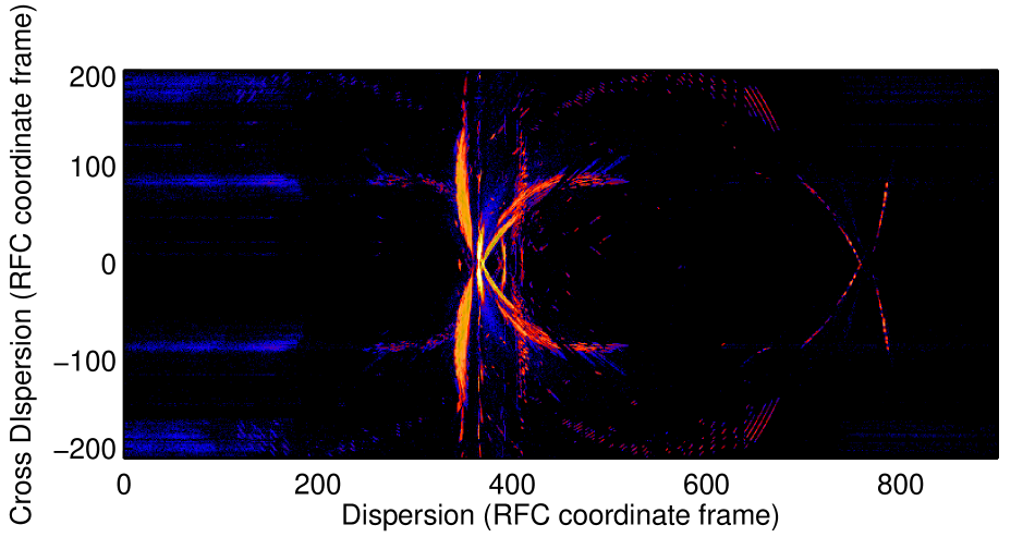
Figure 20: Simulated image for a source at -1.5 degree off-axis in the direction of increasing incident angle on the grating. The projected photons near Z=400 (the narrow lines) are double reflections from the mirror. The fan like shape is due to single or double reflections from the mirror and a single reflections from the grating. In the RFC coordinate frame position (0,0) is de center of CCD5 which is the position of the grating first order blaze wavelength. The coordinates are in units of 0.01 mm.

Based on simulations we calculate the corresponding effective area for different off-axis angles and position on the detector. This is shown in Fig. 21. Based on this sensitivity we verified whether possible contributions from the sky would affect the RGS response. As expected contributions from bright stars dominate the sensitivity, relative to the night glow features and diffuse night sky. Very bright stars near the field of view can be avoided by proper scheduling, as the optical sensitivity depends only on the incident angle with respect to the gratings. Without further scheduling constraints to m_v $\leq$ 5, 4% of the observations would be optically contaminated. Also the population of weaker field stars adds to the optical contamination. Reduction of the optical load is required to keep the contribution of this specular reflected star light to less than 1 electron per readout. This reduction varies from 10^-4 near the optical axis to 10^-2 for the CCDs at the largest distance to the optical axis and has been achieved by an Al layer deposited directly on the CCDs. To compensate for the difference in sensitivity as function of the dispersion direction, we used a thicknesses of 75 nm for CCD9 and CCD8, 68 nm for CCD7, CCD6 and CCD5, and 45 nm for the other CCDs.

Figure 21: Global stray light sensitivity of RGS as modified by the varying Al filter thicknesses (in nm). Separate CCDs and their Al filter thicknesses are indicated (top). The sensitivity for focused (solid line) and non focused light (dashed line) is given separately. The asterisks indicate ray-trace model calculations for the indicated positions on the CCDs.

The suppression of UV/optical light was verified in orbit by observing Canopus an F0 star with m_v = –0.72 between –3 and +2 degree off axis along the dispersion direction. The observed image (Fig. 22) has the correct shape and its intensity is within a factor 2 from the model. Considering the approximations used (a 1 nm change in Al filter thickness may change the transmission up to 15%) this is reasonable and the observation strategy of an avoidance angle for bright sources is sufficient to neglect the effect of optical/UV light on the detector response.

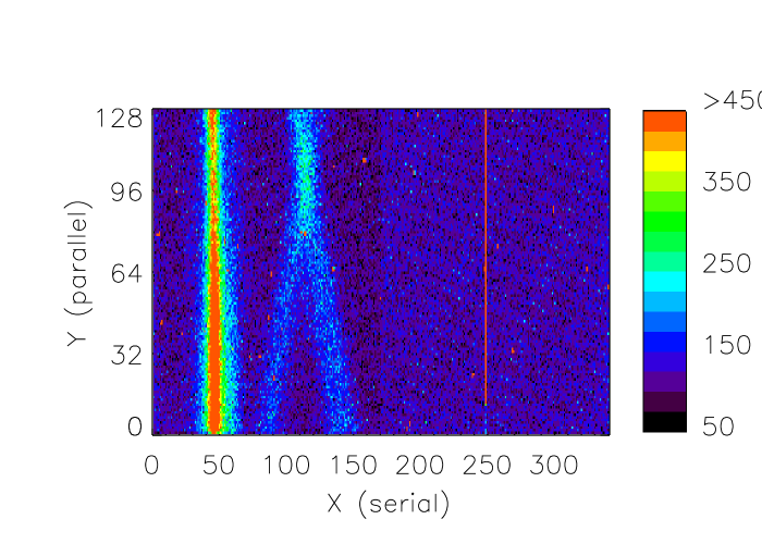
Figure 22: Recorded intensity distribution on CCD 3 with Canopus at -2 degree off axis

5.8 Stability detector response

After applying all correction factors for the evolution of the detector response (CTI, gain, hot columns, read-out noise and dark current and the evolution of hot pixels and columns) we expect that the calibrated CCD response is accurate over the lifetime of the mission. For a detector behind a dispersive element this can be easily verified as the incident energy of each photon is known. In Fig. 23 we show the calibrated CCD redistribution function for one energy at the start of the mission and after 10 years in operations.

Figure 23: In-orbit CCD response at $\beta$ = 0.0715 radians (C VI line) for Capella observations in orbit 54 and 1961. The errors are only shown for orbit 54.

The stability of the detector response, after applying the appropriate corrections is very good and the effect on the effective area is negligible ($<0.25$ %) assuming that the proper pulse height selection windows $\geq$ 95 % are applied.

6 Gratings

6.1 Grating model

The grating response describes the intensity distribution of monochromatic radiation as function of outgoing angle $\beta$ and its component perpendicular to it. The two major contributions are the flatness and the scattering properties of the gratings. Also the grating to grating alignment is a major component.

From scalar diffraction theory one can calculate the total integrated scatter (TIS) out of the line core (kahn1996). This is given approximately by:

$$TIS\leavevmode\nobreak\ =\leavevmode\nobreak\ k^{2}\leavevmode\nobreak\ \sigma^{2}\leavevmode\nobreak\ ({\rm sin}\,\alpha+{\rm sin}\,\beta)^{2}$$ (13)

where $k=2\pi/\lambda$ is the wave number of the radiation and $\sigma^{2}$ is the mean square deviation of the surface which follows from a simple analytical function that is characterized by $\sigma$ and a scale length $l$. This expression (13) is valid in the small amplitude limit where $\lambda>>\sigma\,{\rm sin}(\alpha)$ and where the deflection angles of the surface are small compared to the critical graze angle for reflection. We get a good description of the grating response using two components: an incoherent large scale component with a correlation length of $1\leavevmode\nobreak\ \mu$m and an rms of 8 to 14 Å depending on the grating master and a coherent short scale component with a correlation length of 0.29 $\mu$m and an rms of 15 Å. This second component is due to a sinusoidal wave on top of the groove structure and has been verified by Scanning Tunneling Micrograph images.

For the diffraction efficiency we use an exact approach which solves the vector electromagnetic equations in the space above the grating subject to the periodic continuity relations imposed by the groove surface. Based on synchrotron measurements we verified the blaze angle, which is the angle where the efficiency peaks.

6.2 Gratings calibrations

Calibrations of the gratings included two steps: (a) verification of the grating response model at a synchrotron and (b) measurements of the efficiency of each grating separately at a few wavelengths.

The single grating response was verified by measuring the efficiency of a single grating at the Bessy synchrotron facility in Berlin (Fig. 24). Clearly there is good agreement, allowing the blaze angle and the scattering contributions as free parameters. Near the oxygen and carbon edges a thin layer of hydrocarbons on the surface of the grating is not included in our model, causing small differences. At short wavelengths the model, based on a scalar approximation of the diffraction theory (Cottam1998) breaks down.

Figure 24: Efficiencies for first and second order as measured (solid curve) and as modeled (dashed curve), for a single grating (herder).

All gratings were calibrated as part of the screening of replicated gratings: their efficiency was measured at 8.34 (Al-K$\alpha$), 13.34 (Cu-L$\alpha$), 17.59 (Fe-L$\alpha$) and 23.62 Å (O-K$\alpha$) and scattering measurements were performed at the Al-K line. For a few gratings additional measurements of the inter-order scattering were carried out. The selection of flight gratings was based on a grading scheme where poorer candidates were rejected on the basis of their $m=-1$ efficiencies and the replica flatness (for RGS1: $\epsilon_{\rm Al}>0.09$ or $\epsilon_{\rm Cu}>0.15$ and flatness $<15\>\mu$rad and for RGS2: $\epsilon_{\rm Al}>0.085$ or $\epsilon_{\rm Cu}>0.15$ and flatness $<9\>\mu$rad).

The integrated reflection grating assembly was tested at the Panter facility at MPE. This test included two components: checking the grating assembly by partial illumination of the RGA and measuring the LSF (mirror + gratings) at some energies.

The partial illumination was achieved by blocking the mirror entrance aperture except for a small section, using the so-called Glücksrad. Following these tests we concluded that apparently the reference point for this RGA was not set properly during assembly. This meant that for the first RGA we had to modify the orientation of the RGA with respect to the mirrors by a change in angle ($\Delta\alpha$ = + 4.56 arcmin and $\Delta x$ = 7 mm). In addition a rotation in the cross dispersion direction, around the Z-axis, was applied to reduce the scattering from the supporting ribs on the gratings ($\Delta\theta$ = + 1.71 arcmin). For the second unit such modification was not required. Following these modifications the alignment of the gratings was tested at the Panter long beam facility at MPE and these were consistent with the expected results.

The full verification of the LSF is described in section 7 where we show the results for the calibrations of the mirror and grating combination.

6.3 In-orbit grating response verification

The grating response in the dispersion direction is not easily verified in flight as it includes a convolution with the incident spectral shape of the observed object. When the spectral continuum has a strong gradient, or strong lines are present, spectral intensity will spill to neighboring energy bands and mix with the grating response when the spectrum is integrated in cross dispersion direction along the dispersion axis. A major factor in the grating response is the scattering by the grating due to irregularities and surface roughness of the grating (see Fig. 28).

The grating response was first verified using Mrk 421 for a number of selections in the dispersion angle $\beta$ and in pulse height (Figs. 26 and 25). The spectrum as a function of dispersion angle ($\beta$) clearly shows the different orders and the scattering from the gratings in between the orders. There is good agreement between the data and the modeled response for the first and second order after applying the scattering component.

This scattering also occurs in the cross-dispersion direction. In the two-dimensional data slice of cross-dispersion versus the dispersion, or spectral axes, the cross dispersion profile is affected by the scattering of neighboring spectral bin intensities. However, its fractional amplitude is suppressed by a factor of $\sim 20$ compared to the scattering amplitude along the dispersion direction due to the difference in relative incidence angle between the dispersion and cross-dispersion direction. When the spectrum is collapsed on the cross dispersion axis the cross-dispersion profile is largely a convolution of the mirror PSF with the grating response. Fig. 27 shows the verification of this scattering component. Overall, good agreement is observed, confirming the validity of our scattering model.

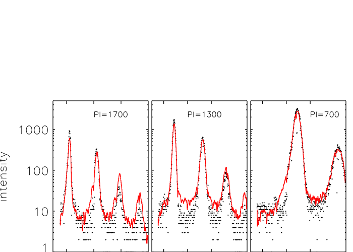
Figure 25: Modeled and measured $\beta$ distributions for given energies expressed in CCD pulse height (PI), where 1 ADU $\approx$ 1 eV. This corresponds to a horizontal slice through the PHA-Beta plot in Fig 2. The peaks correspond to the different orders, starting from order -1 on the left of each plot.

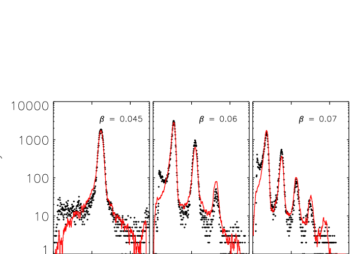
Figure 26: Modeled and measured CCD pulse height distributions expressed in CCD pulse height (PI), where 1 ADU $\approx$ 1 eV, for given $\beta$ angles in radians. This corresponds to vertical slices in the PHA-Beta plot in Fig 2. The peaks correspond to the different orders, starting from order -1 on the left of each plot.

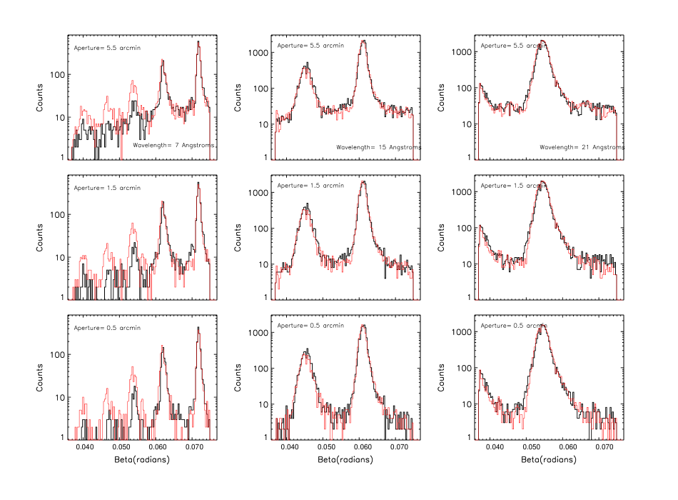
Figure 27: Comparison of modeled response (red line) with observations (black line) for different cross dispersion apertures (ranging from 0.5 to 5.5 arcmin, bottom to top), shown as intensities versus dispersion angle (Beta) for different CCD pulse height selections (columns left to right) at 7, 15 and 21 Å, or 1.7, 0.8 and 0.6 keV.

6.4 Scattering of low energy protons

The low energy protons encountered by XMM-Newton during its orbit form a potential risk for the performance of the CCD detectors (see section 5.2). These protons are scattered and focused by the mirrors onto the XMM-Newton instruments (aschenbach2007). For the RGS an extra reflection by the gratings is required in order for the protons to hit the CCDs. To estimate the efficiency of this process, a sample grating was put in a soft proton beam at the Harvard university, Cambridge accelerator for materials science (rasmussen1999). It was found that for protons of 1.3 MeV, the CCDs would acquire per ${\rm cm}^{2}$ only $10^{-5}$ part of the radiation dose on the mirror entrance due to scattering off the grating.

It was concluded that for the RGS the required extra reflection by the gratings, in combination with the lower vulnerability of our back illuminated devices for these soft protons, offers sufficient protection. In principle the instrument can even be left in operational mode during the periods of high radiation caused by soft protons.

7 Line Spread Function

The line spread function (LSF) is determined by folding of the mirror response with the grating response, taking into account the effect of data selections in the detector. This is schematically illustrated in Fig. 28 where the different components are shown. The sharp symmetric Lorentzian profile describes the mirror response. After folding with the grating response the distribution shows a narrow angle scattering component (Gaussian shoulders in the distribution) and additional large angle scattering wings. The downward spikes in this spectrum are due to discarded hot columns. The small step function is due to the limited range over which certain scattering components are computed. Beyond this range this component becomes insignificant, and only the total wide angle scattering flux is needed to compute the total amount of flux lost from the center of the distribution, to get the proper effective area. Applying the data selection of the CCD the shape of this distribution becomes asymmetric in the wings.

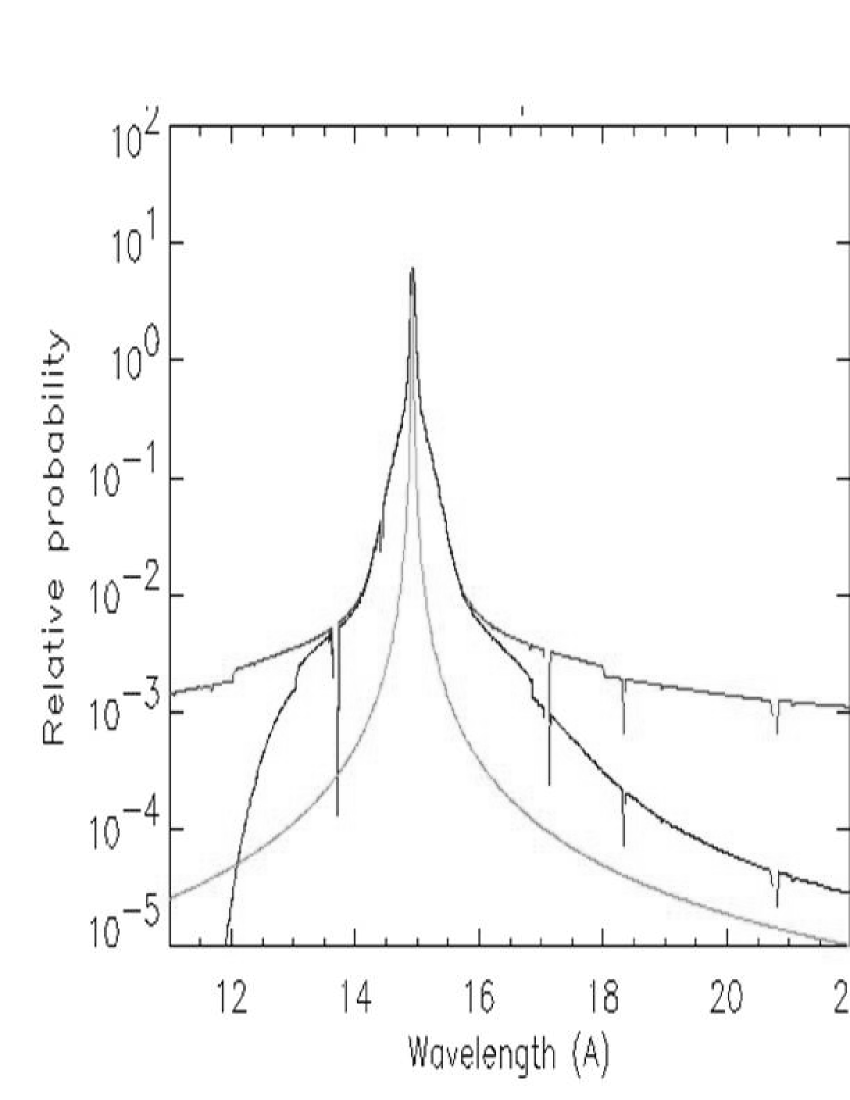
Figure 28: Modeled line spread function showing the different contributions of the mirror (narrow peak), convolved with the small angle scattering (middle line) and wide angle scattering (top line).

The LSF was verified in various stellar sources (Capella, Procyon, HR1099, AT Mic and $\lambda$ And). The instrument behaves slightly better than predicted by the folded responses, in the sense that the line peak is slightly narrower. This is modeled by a small ($\approx 1$ mÅ equivalent for $1^{\rm st}$ order) manual modification of the figure parameters of the grating description (see LINESPREADFUNC ccf calibration file).

A typical example of the LSF response is shown in Fig. 29. The estimated contribution due to the background and the stellar continuum causes the largest uncertainty in the modeled wings of the line.

Using relatively clean emission lines (Ne x ${\rm Ly}\alpha$, O viii ${\rm Ly}\alpha$, Fe xvii, N vii ${\rm Ly}\alpha$, and C vi ${\rm Ly}\alpha$) we determined the resolving power ${\rm E}/\Delta{\rm E}$ for the two orders in the different instruments (Fig. 30). The resolving power is between 100 and 600 in the first order and is two times better in the second order.

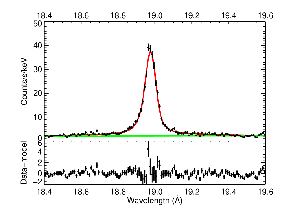
Figure 29: Measured (points) and modeled line spread function (line) for the O viii ${\rm Ly}\alpha$  line in HR 1099 (18.97 Å), for RGS2. The assumed stellar continuum background is indicated by the lower (green) line. The modeled line is shifted by 5 mÅ, to fit the measured line position. This 5 mÅ shift is within the wavelength uncertainty and of the same order as the radial velocity shifts within the system which are between +40 and -65 km/s (Bopp1976), or about $\pm 3$ mÅ. The difference between the model and the data is shown in the bottom plot.

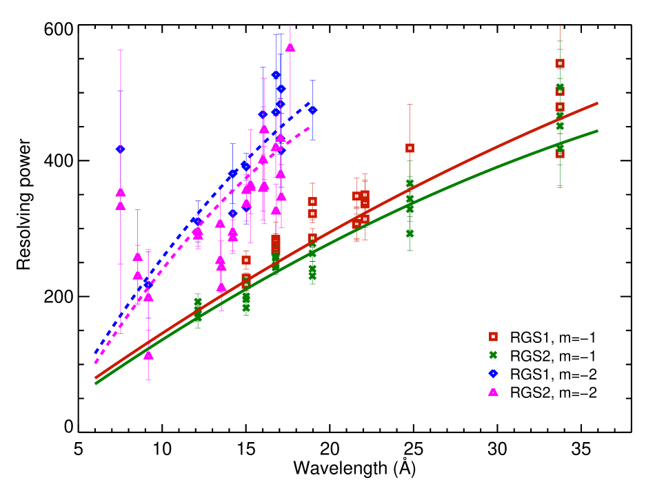
Figure 30: Resolving power for RGS1 and RGS2 implemented in the calibration given by the response matrix (lines), and measured from individual line profiles (points), showing the spread around the model, and demonstrating that the line widths follow the trends defined by the physical model of the instrument.

The modeled LSF and the observed LSF agree well after application of a correction factor for the internal alignment of the gratings of RGS1. Based on the spread of the measured resolution for a given wavelength (Fig. 30) astrophysical line broadening of more than $\Delta\lambda=6$ mÅ or 10 % of the line width of the instrumental profile can be detected significantly for strong lines (${\rm S/N}\gtrsim 25$).

8 Wavelength calibration

On the ground a full calibration of the wavelength scale with X-rays was not possible as the mirror–grating–detector combination has to be at different positions due to the finite source distance at the Panter facility at MPE. Therefore the wavelength calibration had to be performed in orbit.

8.1 Wavelength scale

Using a set of well defined emission lines the relative alignment of the three components, mirror, gratings and detector, has been determined. We have used relatively clean lines (Table 9) in a number of coronal sources during the performance verification phase: Capella (orbit 042, 046, 054), HR 1099 (orbit 025, 028, 031, 036) and AB Dor (orbit 091). In this analysis the barycenter corrections and corrections for the velocity of the spacecraft are included. Since SAS version 13 these corrections can be applied (but not by default) by the standard software analysis system.

Table 9: Lines used to calibrate the wavelength scale and LSF. The last two columns indicate which lines have also been used for the separate RGS1 and RGS2 LSF calibrations.

line	$\lambda_{\rm Laboratory}$	RGS1 LSF	RGS2 LSF
Mg xii ${\rm Ly}\alpha$	8.41	no	no
Ne x ${\rm Ly}\alpha$	12.134	no	yes
Fe xvii	15.015	yes	yes
Fe xvii	16.777	yes	no
O viii ${\rm Ly}\alpha$	18.969	yes	yes
O vii w	21.602	yes	no
O vii	22.101	yes	no
N vii	24.781	no	yes
C vi ${\rm Ly}\alpha$	33.736	yes	yes

The dominant factors in the wavelength scale are (a) actual pointing position relative to the source, (b) a rotation of the RGA around the Y-axis (changing the incident angle) and (c) a linear shift in the Z-direction (dispersion). This is an over constrained problem because the final shift in wavelength depends on a linear combination of ${\rm sin}\,\alpha$ and ${\rm sin}\,\beta$. We have chosen a solution where we fixed the incident angle on the gratings to the preflight calibrations, and modified the offset pointing (boresight) and the shift of the detector (810 and 490 $\mu$m for RGS1 and RGS2 respectively).

It was noted that the variation between observed and theoretical line positions was larger than expected based on the built accuracies of the instrument. Bending of the telescope tube, the structure between the mirror platform and the detector, could have caused this variation. However, this was ruled out because the focus of the mirrors, as recorded by the EPIC instrument, is perfectly stable. After collecting a large set of observations this variation turned out to depend on the angular distance between the Sun and the spacecraft pointing direction, the ”Sun angle” (SA). Considering that the mirrors are mounted at the intersection plane between the paraboloid and hyperboloid, a difference in temperature of less than 0.5 degree between observations with a different SA can explain a shift of up to 2 mÅ. This is well within the required temperature stability of the satellite of 1 degree for the mirror and grating combination. This effect is included in the calibration since version 13 of the SAS. In Fig. 31 the accuracy of the wavelength scale is illustrated. Clearly there is no wavelength dependency after the calibration has been applied.

Recently it was discovered that there appears to be a seasonal pattern in the XMM-Newton pointing accuracy, with an amplitude of 1–1.5 arcsec. This bore-sight variability, originally noted in the EPIC instruments, is thought to be caused by star-tracker instabilities. These offsets are taken into account since September 2012.

Figure 31: Difference between expected and observed wavelengths as a function of expected wavelengths for RGS1 (squares) and RGS2 (triangles). RGS2 data have been slightly (horizontally) displaced for clarity. Error bars are the standard deviations of the statistics of the line fits. The spread of the data points seems somewhat smaller than the error bars indicate. There is a possibility this is due to correlations between spectral bins because of rebinning of the original CCD pixels, which might cause the statistical error to be somewhat overestimated.

8.2 Wavelength accuracy

To verify the ultimate accuracy of the wavelength calibration we have used the same lines for a large number of observations of 4 coronal sources and calculated the distribution of the difference between the expected and measured positions for the first and second order lines (Fig. 32). Table 10 shows the accuracies and line shifts obtained for the lines used in the calibrations. Applying all known corrections, shown in the last column of Table 10, line shifts are zero with a spread for first order of 5 mÅ. Thus for any observed line we expect to know its position with an accuracy of 5 mÅ (1 $\sigma$) corresponding to typically 75 km/s, at 20 Å.

Further improvements can be made when lines are observed in both first and second order. The angle of incidence on the grating for the particular observation can be independently solved by forcing the corresponding first and second order lines to have the same observed wavelength.

The pointing accuracy of the XMM-Newton telescope is 1.5 arc seconds, which corresponds to about 3 mA in the dispersion coordinate. In addition, the emission lines of most coronal sources, due to the violent processes in the coronae and/or the existence of companion stars have velocity uncertainties of 40–50 km/s or about 3 mA. The accuracy of our current wavelength calibration is very close to this theoretical limit of about 4.5 mA.

Table 10: Wavelength accuracy in mÅ for the applied corrections

spectrum	a	b	c
RGS1 order 1	$4\pm 8$	$2\pm 7$	$0\pm 6$
RGS2 order 1	$9\pm 8$	$7\pm 7$	$0\pm 6$
RGS1 order 2	$2\pm 5$	$1\pm 5$	$1\pm 5$
RGS2 order 2	$4\pm 5$	$3\pm 4$	$0\pm 4$

1. Fixed Bore-sight, no further corrections

2. Fixed Bore-sight + barycenter and stellar velocity corrections

3. Variable Bore-sight + barycenter and stellar velocity corrections and Sun angle (SA) corrections

Figure 32: Distribution of the difference between the measured and the theoretical wavelength for nine emission lines in 56 observations of four stars (Capella, AB Dor, HR 1099 and Procyon).

9 Effective area

9.1 Effective area model and ground calibrations

The effective area is a combination of the mirror effective area, the grating efficiency and scattering and the detector quantum efficiency together with any data selection applied. In Fig. 33 the results of the end-to-end tests at the Panter facility are displayed including the expected effective area. The data are corrected for the finite source distance.

Figure 33: Effective area verified pre flight by end-to-end measurements at the Panter facility (herder). This can be compared with the measured in flight effective area as verified on celestial sources (Fig 34). The model is indicated by the solid line. Sharp features are caused by either atomic absorption edges or differences between different CCD Al layers. The broken lines indicate the relevant atomic edges. The asterisk symbols show the measured data points.

These results indicate a 10% accurate calibration of the effective area over the 10–25 Å range. At shorter wavelengths there is a steep gradient in the grating efficiency, resulting in a significantly larger uncertainty of the effective area. At the longest wavelength the CCD QE is less accurately known, up to 40 % (see Figure 9). The longest wavelength point in Fig. 33 is well beyond the maximum wavelength of 38 Å for the in flight configuration of the RGS instruments.

9.2 In orbit scaling

Figure 34: Effective area for RGS1 (black) and RGS2 (red) (two orders) as calculated by the SAS, based on in flight calibrations on celestial sources. Apart of the two failing chains (CCD4 in RGS2 and CCD7 in RGS1) the CCD boundaries can be easily identified. In addition the effect of hot pixels and columns can be seen.

Considerable effort was invested to improve the effective area in orbit by observing continuum sources with good statistics. A total of 1 Ms observations of Mrk 421, PKS 2155-304 and other selected sources (e.g. Vela pulsar, Sco X-1 off axis) are used. The resulting area result is shown in Fig 34. All modifications of the area model are needed due to either uncertainty in the model response or items not fully included in the calibrations.

An unexpected vignetting of the beam was deduced by comparison of the RGS1 and RGS2 response. After launch it turned out that the effective area for RGS1 was less than that for RGS2 and that it scaled with the angle $\beta$ of the dispersed rays ($A_{\rm eff}(RGS1)/A_{\rm eff}(RGS2)=1$ for $\beta=0.036$ and 0.8 for $\beta=0.072$). This dependency is consistent with a partial blocking of the through beam between the mirrors and the RFC and is explained by a 180^∘ rotated baffle of the grating assembly around the optical axis. The purpose of this baffle is to isolate the RGA thermally from its environment. The exit opening is asymmetric with respect to the mirror optical axis to allow an unblocked view to the RGS camera. Although this should have been checked during integration, from a manufacturing point of view rotation over 180^∘ around the optical axis cannot be excluded. The RGS1 effective area is corrected for this using a linear function of $\beta$.

The QE of CCD2 in RGS2 was modified based on continuum spectra of Mrk 421 and PKS 2155-304. In the initial data an unexpected jump in the spectrum was observed for CCD2 in RGS2. The observed loss of QE can be explained and is modeled with an additional 40 nm layer of ${\rm SiO}_{2}$ on the CCD. This layer does match the observed absorption in both first and second orders. Why such an extra layer of ${\rm SiO}_{2}$ should exist on this CCD however, is not clear, and there may be another (unknown) cause for the observed loss in QE.

Systematic flux variations (up to 10% of the flux) on scales of a few Ångstroms, as function of wavelength were observed for sources which are expected to show smooth, power law spectra (e.g. PKS 2155-304, Mrk 421). These deviations from the expected power laws are attributed to unaccounted variations of the effective area. To correct these flux variations, we took high statistics observations of Mrk 421 in orbits 84, 259, 546, 720 and 1084 and fitted absorbed power law spectra to the observations in the interval from 10 to 25 Å. For each spectrum different power law indices and normalizations were allowed, but only one ${\rm N}_{\rm H}$ column density for the interstellar absorption. Thus the source was allowed to vary between observations, but the interstellar absorption remained constant. The same set of parameters was fitted to both RGS1 and RGS2 spectra. It is assumed that in the interval between 10 and 25 Å the effective area of the RGSs is known best, and that in this RGS wavelength interval Mrk421 shows a smooth power law spectrum.

Next the fitted power law and absorption model parameters were frozen and $12^{\rm th}$ order Chebychev polynomials (which could follow the few Å scale variations) were fitted over the full 5 to 38 Å interval to the fit residuals for each RGS separately, but identical for all observations. These Chebychev polynomials are now used as corrections on our effective area and are included in the SAS calibration files.

The second order effective area is normalized using the first order spectra, because the main emphasis of the ground calibrations has been the first order only. The effect of this correction, which is similar for RGS1 and RGS2, is typically of the order of 20 % except at very short wavelengths (see Fig. 35) and is well within the uncertainties of our theoretical model.

Figure 35: Correction factor for the m = –2 spectra relative to the m = –1 spectra (identical for RGS1 and RGS2).

9.3 Instrumental absorption edges

Oxygen edge: The instrument turned out to have a significantly larger instrumental oxygen edge in orbit than anticipated. Some of this is due to oxygen contamination of the optics (see Fig. 24 for example), but a major contribution is on the detector itself. Following launch the detector has always been cooled: before the detector was opened its temperature was –50^∘C while following the opening of the detector the temperature dropped to –80^∘ and subsequently around orbits 532–537 it was cooled to –110^∘C. In practice this means that any contaminating water ice, present on the detector body during launch, would have remained on the detector and has never evaporated.

In orbit the oxygen contamination has been determined using relatively smooth continuum spectra. The oxygen absorption feature is illustrated in Fig. 36 where the spectrum for the combined data of two BL Lac objects with low extinction are shown (172 ks for Mrk 421 and 346 ks for PKS 2155-304) as well as the expected interstellar medium (ISM) extinction. There is a clear mismatch. Comparing these data with sources with high extinction (Sco X-1) it is possible to deduce the instrumental response over the O-edge. The result is shown in Fig. 37. See devries2003 for details. In the observed data the sharp features in this figure will be convolved with the broader instrument response. Applying this instrumental correction to the low extinction data improves the description considerably (see Fig. 36). The feature at 22.77 Å visible in this figure is not present in a number of other spectra (Sco X-1, 4U 0614+19) and is therefore assumed to have an astrophysical origin.

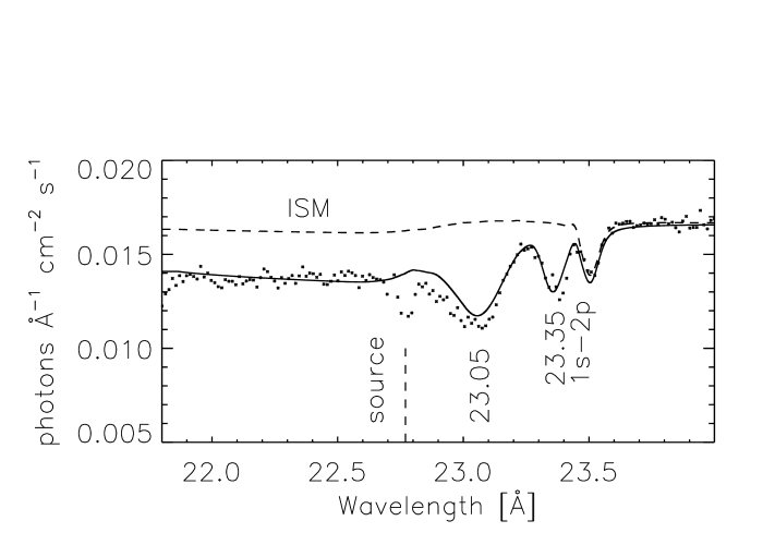
Figure 36: Combined spectrum around the O-edge for Mrk 421 and PKS 2155-304 with the expected absorption from the ISM alone (dashed line) and in combination with the the instrumental component (solid). The feature at 22.7 Å  is not visible in other sources and is therefore of astrophysical origin.

Figure 37: Instrumental efficiency around the O-edge

Fluor and magnesium edges: On the CCD detectors there is a MgF₂ layer, which electrically isolates the optical Al filter from the CCD. This layer will give rise to Mg and F absorption edges in the spectrum. By taking combinations of deep spectra of continuum power law sources (Mrk 421, PKS 2155-304) and assuming no astrophysical features were present around the Mg and F edges, the details of these edges were measured. The Mg edge follows with sufficient accuracy the edge predicted by Henke, but the F edge shows deviations. The depth of the edge agrees with the depth predicted by Henke and the known thickness of the MgF₂ layer, but the shape of the edge is different. This fitted shape is included in the effective area calibrations used by the SAS.

9.4 Hot pixels

In hot pixels the charge sometimes tends to overflow along the column to neighboring pixels. When pixels are only occasionally hot during an observation, these pixels are not recognized as such, but the set of neighboring pixels in a frame will be recognized by the onboard processing, and discarded as being a ’complicated’ event or cosmic ray. Such discarded pixels are not individually flagged, but only the average decrease in effective area of the whole CCD is recorded. Hence holes, or ’cool’ pixels, appear in the processed spectra as narrow ’absorption’ features, due to the unrecognized loss of effective area for some columns. A typical ’cool’ column is shown in Fig. 38.

When searching for weak absorption features, it is important that these effects are taken into account. A list of pixels and columns is maintained in the calibration files (the ’COOLPIX’ ccf). In the ground processing software (SAS) there is an option to include or exclude these known pixels. For individual observations, redundancy of both RGS instruments may allows us to identify these columns in the individual instruments. In addition spectra of first and second order are compared to reject absorption features which occur at the same spot on the CCD, which is at half the wavelength in second order. Furthermore the multiple pointing mode (section 11.2) helps to mitigate this problem.

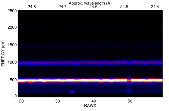
Figure 38: Signature of a cool column on CCD4 of RGS1 (1 Ms Mrk 421 data summed in detector space in a plot of pulse-height (Energy) versus dispersion axis. Top curve is the second order of the dispersed spectrum, while bottom curve shows first order. A ”cool” column can be recognized around RAWX=50, or about 24.5 Å in first order. This column extends into second order at the same position, but at half the wavelength. Top scale is the approximate wavelength of the first order only.

9.5 Contamination

Prior to launch the camera was purged with clean N₂ and its door was sealed. Between this sealing and the launch many months passed. In this period water vapor may have entered the cavity of the CCD detectors, especially during the time on the launch platform in the very warm and humid air at the tropical launch site of Kourou, French Guiana.

Following the launch the instrument was passively cooled to –50^∘C and stayed at this temperature until the opening of the detector door. Hence it is not surprising that a considerable oxygen edge is observed in the instrument response (see section 9.3). Although the instrument has the capability to be heated up to around 45 ^∘C this has not been exercised as it is virtually impossible to predict accurately what happens to the instrument which has stayed cool for over 14 years. In addition any contaminants, when evaporated, will largely stay inside the telescope tube and hence will condense again at a later stage.

The depth of the oxygen edge is very stable over time (see Fig. 39). Apparently the contamination with water ice indeed was a single event, and a single calibration (section 9.3) suffices to correct for this effect.

However, monitoring of two stable sources (RX J1865.5-3754 and the Vela pulsar) shows that the response of the instrument at long wavelengths suffers from loss of effective area, which increases over time. This is thought to be caused by a second contamination component: out-gassing of hydrocarbons by the carbon-fiber structures of the telescope tube, although great care has been taken with selection of the materials. A special cold section at –80 ^∘C is present in the telescope tube to freeze contaminants, and an out-gassing vent port is present to release any remaining contaminants to open space. However contamination of the RGS CCD detectors cannot be prevented because the CCDs are the coldest structures (–110 ^∘C) and completely open to the telescope tube. By contrast, the EPIC cameras usually have optical blocking filters in front of them, which are at higher temperatures, and protect their CCDs. In addition, contaminating layers may also form on the optics (mirror and gratings), which will have the same effect.

Assuming perfect stability of the calibration sources RX J1865.5-3754 and the Vela pulsar at long wavelengths, the thickness of the contaminating layer can be calibrated. Assuming a type of hydrocarbon as ${\rm C}_{8}{\rm H}_{8}$ to be representative for the contaminating compound(s), Fig. 40 shows its measured thickness with time. After an initial increase of the carbon layer on the detector, the increase now levels off as the mission progresses. For revolution 2200 a reduction of 47% of the detector response at 35 Å is observed. At shorter wavelengths, this reduction is smaller e.g. 35% at 30 Å, and 24% at 25 Å. This reduction of effective area is taken into account during standard processing.

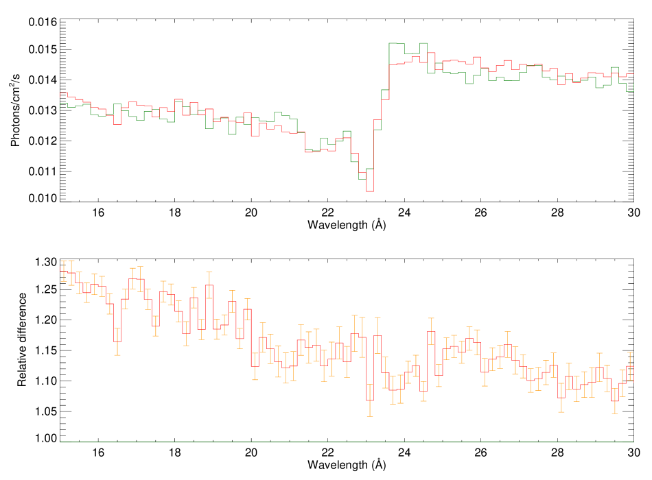
Figure 39: Stability of the instrumental oxygen edge: comparison of spectra corrected for a change in slope and normalization (top) and ratio (bottom) of Mrk 421 data in orbit 84 (red) and orbit 2002 (green). The spectra show the uncorrected instrumental edge, which is normally corrected for during default data processing. The slight linear trend in the relative difference plot(bottom) is caused by small changes in the source power law spectrum over time.

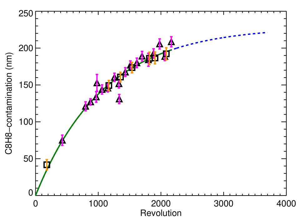
Figure 40: Contamination history given in units of C8H8 thickness, $\rho$ = 1.11 ${\rm g/cm}^{3}$. Triangle data points are the RX J1856.5-3754 data points, while the square points are the Vela pulsar data points. The broken line is the prediction of the contamination for the near future.

Using the onboard calibration sources in principle the contamination of the CCDs can be verified independently. This is however complicated because the calibration source, a Cm²⁴⁴ $\alpha$ emitting source, is also cool and contaminated. Hence contamination of the source or of the target will effectively lower this count rate more than is expected based on the radioactive decay time of the source itself. Especially the alpha particles of the radio-active source, which are generating the X-ray fluorescent photons on the F and Al targets, are very susceptible to small amounts of contamination. This is illustrated in Figs.  41 and  42. In addition, the hydrocarbon contamination will mainly affect the longest wavelengths but the Fluor-K line and the Al-K line are at shorter wavelength (18.30 and 8.33 Å, respectively) and hence far less sensitive to contamination than the astrophysical calibration sources at 32 to 37 Å.

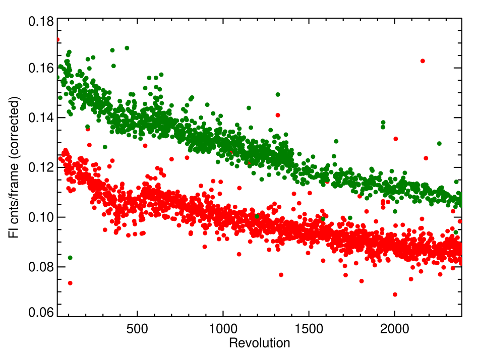
Figure 41: Onboard calibration source count rate for the Fluor source after correction for source decay time and CCD hot pixels and columns. Red data points is RGS1, green data points is RGS2.

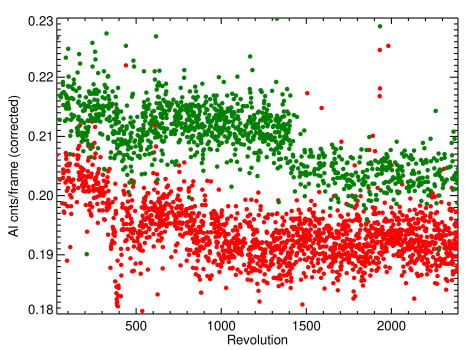
Figure 42: Onboard calibration source count rate for the Al source after correction for source decay time and CCD hot pixels and columns. Red data points is RGS1, green data points is RGS2. The drop in RGS2 count rate around orbit 1405 is due to the switch to single node readout. A smaller drop at the same time is also observed for the fluor source (Fig. 41)

9.6 Pile-up effects

Pile-up, which is the process of two X-ray events hitting the same or neighbouring pixel(s) within one readout frame, has the effect on the effective area of moving two events from e.g. first order into one event in second order. Consequently the effective area of the first order will decrease, while considerable background is added to second order. Fortunately pile-up is negligible for most sources.

Taking observations using different CCD integration times, by using different total number of CCDs in the readout chain, on the same constant source, pile-up can be measured. This way it is estimated that pile-up for the very bright source of the Crab is maximally 14% around 12 Å wavelength (Kaastra2009), when using all CCDs in the default spectroscopy double node readout mode. However, Crab is an extended source. For the bright point source Mrk 421 in a flux state of 450 photons ${\rm m}^{-2}{\rm s}^{-1}{\rm\AA}^{-1}$ at $\lambda=25$ Å, maximum pileup is estimated at about 1% for $\lambda=$16-18 Åfor double node readout. For RGS2 in single node readout, pile-up is worse at about 2.4%. Most sources are much weaker than Mrk 421, and hence pile-up can be ignored.

For very bright sources (e.g. Sco X-1, Cyg X-2) however pile-up can have dramatic effects. When there is considerable pile-up, neighbouring pixels can combine and form ’complex’ patterns, which will be discarded onboard. Hence, holes will appear in the spectrum. There is no way to correct for those. Best is to limit pile-up by using the RGS small window mode (see section 11.2), and/or using only a limited number of CCDs in the readout chain.

9.7 Effective area accuracy

The absolute scale of the RGS effective area was calibrated on the well known source of the Crab pulsar and nebula. This calibration has been described in detail by Kaastra2009. It is estimated that the absolute effective area scale of the RGS is accurate to within the accuracy of the adopted continuum model for the Crab, which is about 10%.

Contrary to most sources, the Crab is an extended source. This has been taken into account into the effective area calibrations, which means that the instrumental models for off axis effective area and cross dispersion scattering were incorporated in the effective area analysis. In addition custom selections had to be applied in the pulse-height versus dispersion coordinate space to prevent inclusion of too much CCD background at long wavelengths and low pulse-height values. Details of this analysis are given in Kaastra2009. For on-axis point sources these effects do not play a role. Crab is also a bright source, which means that pile-up has an effect. As mentioned before, this effect was taken into account.

The redundancy between RGS1 and RGS2 can be used to obtain some idea about small scale systematic uncertainties in the effective area, which define the sensitivity for detecting weak absorption structures. We start with the fluxed spectra ${\rm S}_{\lambda}$, in which all known exposure, bad columns and pointing history effects have been taken into account in the used response. The $\lambda$ bins of the spectrum are sufficiently narrow that they are of the same order as the wavelength range of individual CCD pixels, such that uncalibrated individual pixel effects will show up the the fluxed spectrum. We know that on larger scales ($>1$ Å) residual uncalibrated differences exist in effective area between corresponding bins of RGS1 and RGS2 and hence between the computed fluxes in the spectra. Small scale spectral structures will be retained in the difference $\Delta{\rm S}_{\lambda}$ between the original spectrum ${\rm S}_{\lambda}$ and the 1 Å smoothed (convolved) spectrum ${\rm C}_{1\AA}({\rm S}_{\lambda})$:

$$\Delta{\rm S}_{\lambda}\equiv{\rm S}_{\lambda}-{\rm C}_{1\AA}({\rm S}_{\lambda})$$ (14)

In effect this is a high spatial frequency filtering of the spectrum, which keeps the narrow features, by subtracting the smoothed spectrum in which all features have been smoothed over a sufficiently (1 Å) wide area. For a featureless spectrum, the $\Delta{\rm S}_{\lambda}$ should follow the noise statistics of the spectrum, such that

$$\sigma^{2}=\frac{\sum{(\Delta{\rm S}_{\lambda}-\overline{\Delta{\rm S}_{\lambda}})^{2}}}{N}$$ (15)

where $\overline{\Delta{\rm S}_{\lambda}}$ is the average value for $\Delta{\rm S}_{\lambda}$, which should be around zero, $\sigma^{2}$ the variance of the distribution, and $N$ the number of spectral points. For the individual spectral points ${\rm S}_{\lambda}$ the statistical error $\sigma_{\rm s}$ is known from the photon statistics of the observation. For a featureless spectrum the average error should be identical to the computed sigma: $\sigma=\overline{\sigma_{\rm s}}$, unless systematic effects play a role.

However, we do not know if the spectrum is really featureless. To get an idea of systematics we look at the difference between RGS1 and RGS2. The individual spectra should follow the same true features, and hence these features are eliminated from the difference:

$$\Delta{\rm S}_{\lambda_{12}}\equiv\Delta{\rm S}_{\lambda_{\rm RGS1}}-\Delta{\rm S}_{\lambda_{\rm RGS2}}$$ (16)

The variance of this subtraction ($\sigma_{12}^{2}$) is twice the variance of the individual $\Delta{\rm S}_{\lambda}$:

$${\sigma_{12}}^{2}=\frac{\sum{(\Delta{\rm S}_{\lambda_{12}}-\overline{\Delta{\rm S}_{\lambda_{12}}})^{2}}}{N}=2\cdot\sigma^{2}$$ (17)

Table 11 shows $\sigma$ computed from the RGS1-RGS2 difference, expressed in units of error on the individual spectra points $\sigma_{\rm s}$ for the observed flux in Mrk 421, by combining different sets of observations to obtain different signal to noise ratios of the spectrum. It appears that, when signal to noise increases the $\sigma$ of the distribution becomes larger than the statistical error $\sigma_{\rm s}$ because systematic uncertainty effects, the pixel-to-pixel systematic errors, become more dominant. This means that a larger fraction of pixels will have values outside the statistical expected accuracy (the outliers). This effect should be taking into account when looking for weak line features close to the statistically expected threshold. For signal to noise ratios larger than 10 (100 counts per bin) these effects start to play a role. For signal to noise ratios of around 70, the statistical uncertainty is equal to the systematic uncertainty, translating into about a 1.5% uncertainty in short scale effective area variations.

Table 11: Differences between RGS1 and RGS2 as function of signal to noise ratio per pixel. Differences outside normal Poisson statistics reflect the systematic uncertainties in the effective area accuracy

S/N ratio	difference a	outliers b
	width ($\sigma_{\rm s}$)	(%)
6.7	1.01	0.2
36	1.09	0.3
69	1.41	3.7

• Width of distribution of differences expressed in statistical uncertainty $\sigma_{\rm s}$ of the spectrum. Offsets (constant difference) are ignored.

• Percentage of pixels outside of the $3\sigma_{\rm s}$ statistical uncertainty.

10 Instrumental background

The instrumental background consists of several components, each with their own characteristics and temporal behavior. In the next subsections we will discuss the characteristics and behavior of these components, and the way background can be dealt with in the observational data.

10.1 Soft proton background

The major time dependent component of the instrumental background are the soft protons, trapped in the earth magnetic field and scattered through the XMM optical path. Apart from the potential of causing damage on the CCDs (see sections 6.4 and 5.2), soft protons mainly add a time variable background component on the detectors. Due to the scattering characteristics of the mirrors and gratings, soft protons will have the highest flux closest to the optical axis, on CCD9, decreasing towards CCD1. Selecting data cuts outside the parameter space of the normal X-ray dispersed spectrum on CCD9 provides a high quality monitor on the soft proton flux and the nature of the main instrumental background component. In orbit, the count rate on RGS CCD9 is used as a radiation monitor to warn for high incident proton flux, and is used to activate the protection for the EPIC instruments. Fig. 43 shows the nature of the soft proton flux as counts on the off-source positions, integrated over the full energy range as function of the dispersion axis, comparing a period of high soft proton activity with a period of low activity.

To improve the signal to noise ratio of the processed spectra, the count rate on CCD9 can be used to select periods of low soft proton background. For extended sources, count rates on CCD9 outside the normal spectra pulse height space are used as parameters to construct a background spectrum, based on spectra of empty fields with similar CCD9 count rate (soft proton) parameters. These sets of background spectra for various soft proton backgrounds are maintained as standard calibration files for the RGS processing software (SAS).

10.2 High energy particle background

Soft protons are low energy particles, scattered by the optical components. High energy particles, mainly from solar CME events, simply penetrate through all spacecraft structures, evenly illuminating the RGS CCD detectors. High flux events only occur occasionally and are usually predicted, in which case the instruments are switched off. Those events do however increase the amount of hot pixels and columns and CTI of the CCDs. At all times there is a low flux, high energy particle background. Many of these particles are detected and discarded as events well above the upper energy threshold due to their high energy contents, or are recorded on the CCDs as a track across many pixels, corresponding to the particle path across the CCD, and are discarded by the onboard processing as ’complicated’ events. The average effective area of the CCD is corrected for the pixels discarded in this way. It is thereby assumed that this background does illuminate the CCD evenly. The remainder of these events, which are not recognized as such add a low and flat background component.

10.3 Detector background

The CCD detectors produce low energy system noise and warm/hot pixels. These effects have been described before (sections 5.3 and 5.4). Applying the appropriate selections in data space and on pixel level, this background is minimized.

The calibration sources are a type of background introduced on purpose on the detector. This background is very constant and well known. The main part of this background is discarded by the appropriate selections in data space. The remaining part is perfectly modeled by the standard processing tools.

Another type of detector background is due to fluorescent lines generated by the high energy particles background in the detector housing. This background is variable. Fluorescent lines that can be recognized are the Al-K line because most of the material of the housing is aluminium and the gold-M line because there is a thin layer of gold deposited on the structures surrounding the CCDs. These lines can be recognized in CCD pulse height space only and are constant in dispersion and cross-dispersion directions. Hence they do not show structure in the dispersed X-ray spectrum, but do add e.g. 0.02 cnts/s over the entire CCD detector for the gold-M line.

10.4 X-ray background

The sky itself provides a true X-ray background, consisting of numerous unresolved distant cosmic sources (see e.g. gili2007), and X-ray lines generated locally by e.g. the charge exchange mechanism in the earth vicinity in interplanetary space (see e.g. cox1998; cravens2000; fujimoto2007). For the RGS the X-ray background can be treated as an extended source. X-ray lines from the background will be visible in the RGS spectra as very broad features which follow the effective area as function of dispersion offset. With standard background processing for point sources, which takes the background from off-axis positions in cross dispersion directions and applying the same selections in CCD pulse height space, the X-ray background is perfectly subtracted, since it is identical for source and off-source positions. When applying background models for extended source analysis, discrepancies between X-ray backgrounds from the sky positions from which the models are made with the observed sky position can keep some background signal in the spectrum. That signal however is usually very low.

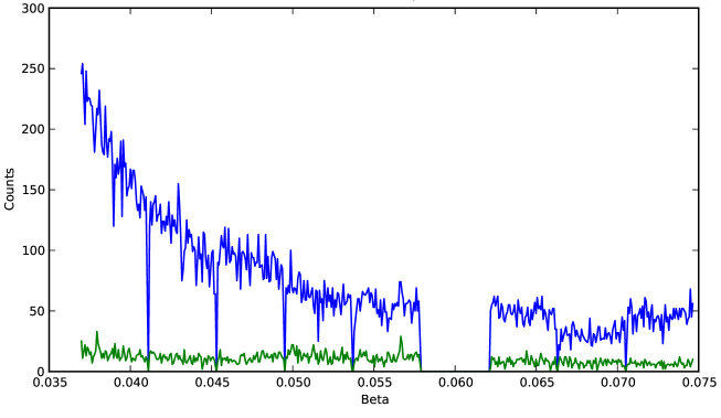
Figure 43: Raw count rate distribution as function of CCD position along the dispersion direction for an off-axis region. The difference between a quiet period (green line) and a high background period (blue line) is in agreement with the expectations. The observations used are from AB Dor, RGS2, revolution 546 (high background) and revolution 668 (low background), with similar cross-dispersion and pulse-height selections for all CCDs.

11 Instrument operations

Instrument operations had a clear impact on the calibrations. Onboard hardware settings affect the efficiency with which the charge can be clocked through the CCD, the selected read-out speed affects the amount of pile-up, onboard event selection parameters influence the number of selected events to be transmitted to the ground and so on. In this section we present the operational aspects of the instrument that affected the calibrations. Table 12 lists the major changes in instrument operations. We first start with the operational conditions that affected the hardware configuration of the instrument.

11.1 Instrument operational conditions

Detector element failures: the read-out channels connected to two CCDs failed over the mission lifetime. The first failure (RGS2 CCD4) was traced back to a frequently used digital hardware switch (HS-202RH) whereas the second failure (RGS1 CCD7) could not be unambiguously traced back to a single hardware component and could also be due to failure in the CCD itself. Due to the complete redundancy between the two instruments, the full wavelength range is still covered. In particular around the Ne x Ly$\alpha$ line and the O vii triplet this has significant impact.

After the second failure it was decided to lower the clock voltages to reduce the load on various electrical components (orbit 168, see Table 12). This tuning resulted in a slightly modified instrument response which can be completely accounted for in the calibrations.

Perigee passage condition: during the initial phase the instrument was powered during the perigee passage. From orbit 171 this powering during perigee passage was stopped because there was concern about the de-rating of some of the electronic components related to the above mentioned failures. Because the instrument behaved stable over many years after this change, this concern was probably not justified.

Detector biasing: Radiation damage at the CCD gate structure translates into a different biasing of the clocks used to transfer the charge through the CCD and thus results into a degradation of the charge transfer efficiency (CTE). By the capability of the instrument to set the clocking voltages in each CCD such degradation can be compensated. Apart from re-tuning to set proper clock voltages following the clock voltage reduction after the RGS1 CCD7 failure, changes in clock voltage settings have only been necessary for one CCD. The clock voltage of RGS2 CCD2 was modified in orbit 1389 (see Table 12).

Cooling: Initially the detectors were operated at –80$\,{}^{\circ}{\rm C}$. This temperature was selected as a compromise between the charge transfer inefficiency (which gets better for temperatures as low as –110$\,{}^{\circ}{\rm C}$  or –120$\,{}^{\circ}{\rm C}$) and the potential contamination on the detector. Because there is no thermal filter between the detector surface and the XMM-Newton telescope tube, the structural element connecting the mirror platform and the detector platform, the camera will act as cryo pump for this volume. The relatively high operational temperature resulted in an increasing number of hot and flickering pixels during the first years in orbit. In orbit 532 and 537 the operating temperatures of the detectors were lowered to –110$\,{}^{\circ}{\rm C}$  to reduce the fraction of hot pixels.

Current limiter RGS2: Each CCD is read out simultaneously through two output amplifiers and only one CCD is read out at a time: while one CCD is read out, the others accumulate data. Upon completion of the read-out, the image section of the next CCD is transferred to the storage section and this next CCD is ready to be read out.

To handle the data streams each camera has two complete read-out chains, which control the clocking of the charge through the CCD, provide the analog to digital conversion and perform data selections to keep the telemetry within reasonable limits. Each read-out chain includes circuits to protect the rest of the system for potential failures. The dimensioning of one of the current limiters in one of the read-out chains (RGS2, node D) was too restrictive to cope with the de-rating of its electrical components beyond the planned lifetime. This happened after about 4 years. Initially the camera continued to operate properly as the current limiter was reset by the ’power-on’ of the CCDs following tripping of the current limiter. Due to the continued degradation of the components, the occurrence of this problem increased and started to affect the measurements; there was a need for more frequent resets. By lowering the temperature of the electronic components ($<$ 4^∘C) the current limiter was pushed back into its operating range. Further degradation of the components required an even lower temperature of the electronics after orbit 1408 (August 27, 2007). This could only be achieved by lowering the temperature of the full focal plane and this would affect the calibrations of the other instruments on XMM-Newton too much. Therefore it was agreed to disable one of the two read-out chains of RGS2 and read its charge through a single output node by changing the clock patterns. The only disadvantage is that this increases the read-out time of all CCDs by approximately a factor 2 resulting in a slightly larger dark current and a larger fraction of piled-up events. For most of the observations, however, the pile-up fraction is very small and therefore the impact is marginal. An unexpected result of this change in read-out was that the fixed pattern noise (see section 5.2) disappeared.

Table 12: Major changes in RGS hardware operations and their scientific impact. At this moment, after 2009 no major changes have been necessary.

orbit	date	event
	yy-mm-dd
24	00-01-25	first light RGS2
26	00-01-30	failure RGS2 CCD4 electronics
		$19.9<\lambda<24.9$ Å
30	00-02-06	first light RGS1
45	00-03-08	upload DPP code (19) for improved onboard particle background data handling. Data $<$ orbit 45 have wrong exposure
52	00-03-21	update IC code (S206): no impact
135	00-09-02	failure of RGS1 CCD7
		($10.3<\lambda<13.6$ Å), RGS operations suspended
147	00-09-26	operations resumed
168	00-11-07	modification of bias settings of RGS to reduce part stress
171	00-11-13	RGS set to setup mode during perigee
192	00-12-25	RGS2:CCD2 bias back to before orbit 168
361	01-11-29	upload IC code (S207): no impact
363	01-12-01	upload IC code (S207): no impact
532	02-11-04	cooling RGS2 to -115∘C
537	02-11-13	cooling RGS1 and RGS2 to -110∘C
538	02-11-15	RGS2 CCD2: serial bias to -2.7 V
584	03-02-15	CSG code (83) : HTR 3x72 mode
765	04-02-13	1st activation of current limiter RGS2
786	04-03-24	2 hot spots in RGS1:CCD1
905	04-11-18	RGS1 upload IC code (S208): no impact
907	04-11-22	RGS2 upload IC code (S208): no impact
1207	06-07-12	lowering temperature electronics to limit impact of current limiter
1389	07-07-11	RGS1 CCD2: serial bias to -4.8 V
1408	07-08-16	single node read-out RGS2
1671	09-01-24	upload CSG code (95): small window mode became available to users after 10-10-8

11.2 Operational settings

In addition to these changes in the hardware configuration, there is a large set of onboard parameters and operating modes which may effect calibrations and/or data quality:

Lower level threshold: The unprocessed data stream from the CCDs is too large to be handled by the onboard electronics. Therefore we reject all bins with a contents consistent with the CCD system level plus dark current and (read-out) noise. This is to so-called rejection threshold.

Hot pixel and column rejection: In addition the pixel coordinates are compared to an uploaded hot pixel/hot column table and are rejected if they are listed in this table.

Event recognition: The remaining data are searched for valid X-ray patterns. Events which spread their charge over an area which extends beyond a 2x2 pixel square are rejected (charged particles or piled-up events). After adding the charge for the remaining valid patterns, only reconstructed events are transmitted to the ground if their charge is above acceptance threshold and below upper threshold. The acceptance thresholds are set such that they approximately follow the lower boundary of the pulse-height distributions of first order dispersed spectral events. These thresholds are set per half of a CCD (CCD-node), and explain the increase of dark areas towards low $\beta$ angle in the bottom panel of Fig. 2.

Instrument modes: The read-out of each CCD can be controlled in great detail. For the RGS operations it turned out that $3\times 3$ onboard binning of the pixels was a good compromise between the read-out speed, the number of hot columns, and the line spread function. For high count rates one can reduce the effect of pile-up, meaning the effect of more than one photon in a bin during the data accumulation, by either reducing the number of CCDs to be read out, or by selecting a smaller region in the cross dispersion direction. This later option, the so-called ”small window mode”, is available from orbit 1671 onward.

Multiple pointing: Despite all calibration efforts it cannot be excluded that there are small temporal unaccounted for CCD pixel to pixel variations in e.g. electric offset and/or charge loss due to evolving CCD damage. This varying CCD response effects the effective area by means of the event selections, and can affect the interpretation and identification of weak emission or absorption lines. By splitting long observations into observations with shorter observation time and using different pointing offsets in steps of 35 mÅ corresponding to steps of 15 arcsec, the detector response can be separated from real features in the observed source. Although this was feasible from the launch onward, from ”call for proposals” AO08, orbit 1693, the so-called multi-pointing mode has been made available to general users. There is no overhead during re-pointing of the telescope, since all data, including the data obtained during the small slews of the telescope, can be used. Locations of X-ray events on the detector are converted into wavelength space, based on telescope pointing reconstruction at the moment of X-ray detection.

11.3 Radiation environment

The radiation environment is characterized by three distinct components: the orbital passage through the radiation belts, coronal mass ejections (CMEs) due to solar activity and regions in the orbit with trapped soft protons. In Fig. 44 two components are shown: the regular transfer through the radiation belts and the presence of one of the major CMEs during the mission lifetime.

Figure 44: Radiation environment for XMM-Newton, as observed by the radiation monitor in orbits 105-120, including 10 perigee passages (indicated) and one of the strongest CME observed.

Perigee passage: Up to orbit 171 the instrument was kept switched on during the perigee passage and indeed the CCDs were completely flooded by charged particles (as could be deduced from the full frame images). After this orbit the instrument was switched off (with the exception of the Digital Electronics) to minimize possible damage by energetic charged particles of the different electronic components.

Solar activity: Fig. 45 shows all solar activity throughout the mission as recorded by the XMM-Newton radiation monitor. In Table 13 we list the major flares. We provide the combined maximum count rate for electrons between 130 keV and 1.5 MeV and protons between 1 and 4.5 MeV during the increased solar activity. Clearly the strong flares last for several up to 15 revolutions. As is indicated in this table, XMM-Newton has experienced 5 major solar flares with log(cnts/s) $\geq$ 4. With use of the OMNI data (see http://omniweb.gsfc.nasa.gov/ow.html) we have calculated the fluence and hardness ratios of these flares. Due to the incompleteness of the data (telemetry) we can only provide lower limits for the fluences but these are reasonably representative as the number of missing data points is limited. For the first 4 major flares the fluences and hardness ratios are given in the table. All other flares are significantly weaker. In section 5.2 we described the effect of these flares on the detector response.

Table 13: Major solar activity, which affected the observations and/or operations

orbit	date	XMM	fluence a	hardness	comment/duration
	yy-mm-dd	log[cnts/s]	($\times 10^{9}$)	ratio b
110	00-07-15	4	1.2	0.48	3 revolutions
169	00-11-10	4	1.6	0.38	1st burst, 13 revolutions
176	00-11-25				2nd burst
239	01-03-30	3			9 revolutions
375	01-12-27	3			1st burst, 12 revolutions
383	02-01-11				2nd burst
433	02-04-21	3			5 revolutions
711	03-10-28	4	1.0	0.28	1st burst, 15 revolutions
723	03-11-20				2nd burst
934	05-01-15	4	0.8	0.25	5 revolutions
1052	05-09-07	3			5 revolutions
1282	06-12-09	3			6 revolutions
2106	11-06-09	3			2 revolutions
2220	12-01-22	3			4 revolutions
2242	12-03-06	4			2 revolutions

• Protons above 2 MeV (lower limit).

• p ($\geq$10 MeV) $/$ p ($\geq$ 2 MeV), with p number of protons.

Figure 45: Count rate outside the radiation belts registered by the XMM-Newton radiation monitor in the high energy ”nhe2” channel (electrons: 1.3-1.75 MeV, protons: 9-37 MeV). This displays the solar activity (spiky structures due to solar flares) throughout the mission, showing the active sun at the start and after 10 years of mission and the solar minimum in between.

Soft protons: In addition to these expected radiation components ’clouds’ of soft protons are present in the environment. Typically their occurrence increases closer to perigee but they can occur in short bursts all over the orbit. In Fig. 46 we show the typical count rates during a random set of orbits. The count rates shown are data collected in the RGS instrument with pulse heights and positions on the detector where no X-rays dispersed from the gratings are collected (regions outside the source position, on CCD 9). Soft protons from outside will be absorbed by the satellite and detector housing but protons entering the telescope mirrors are scattered by the optics and subsequently recorded by the detector (see section 6.4). Therefore this count rate is a reasonable accurate estimate of this background component.

Figure 46: Illustration of soft proton count rates per second in the RGS detector (CCD9 node C, RGS1) for 9 different orbits (displayed with an offset of 2 for clarity)

Seasonal variations: The background rates during passage through the perigee belts shows a clear dependency on the season. During the course of the seasons the relative position of the orbit with respect to the Earth magnetosphere changes. This is illustrated in fig. 47 where the count rate in RGS for $\lambda<7.7$ Å and a selection in the cross-dispersion direction $>1$ arcmin away from the source direction is shown for different phases of the orbit. During the first and last part of the orbit the instruments are switched off since during the perigee passing no science data can be recorded. In addition to reduced background closer to apogee we see also the seasonal effect of the impact of the Earth magnetosphere.

Figure 47: Seasonal variations in the instrument background in counts per second on node C of CCD9, as function of orbit. The different phases of the orbit are shown from bottom to top with a different offset for clarity (indicated by the dashed lines). The phases for the perigee passage are omitted (1/8 and 8/8). The others are shown for increasing phase (bottom to top; for clarity the labels of phases 3/8 to 5/8 are left out). The large scale trend of increasingly smaller maxima in later years, shows the decreasing solar activity over the 11 year solar cycle.

12 Conclusions

Continuous monitoring and special purpose calibration observations of the RGS instruments over the years, since launch, have yielded an accurate calibration and understanding of the instruments. Although many instrument parameters were measured before launch, in flight measurements of celestial sources allowed a far more accurate assessment of these parameters. In addition the behavior of the instrument due to cosmic radiation, temperature and attitude variations, and aging, are now well understood.

The following major aspects of the RGS, described in this paper, can be summarized as follows:

• Detector performance The CCD detectors are subject to damage by cosmic radiation and soft protons. The major effect is the appearance of hot pixels and columns. Cooling the detectors to -110^∘C made most hot pixels disappear and has kept the amount of hot surface limited since then. Unfortunately two different CCDs were lost in the two instruments quite early in the mission, but overlap between the instruments still allows the full spectrum to be measured. Effects of increasing charge transfer inefficiency (CTI) are small ($<10\times 10^{-5}$) and appear not to play a role in the RGS.

• Wavelength scale Although the original calibration kept the wavelength scale accuracy within specification, improvements have been made by taking into account effects of the angle of solar illumination on the spacecraft and seasonal effects in pointing. The blind accuracy of the wavelength scale is now of order 6 mÅ in first order.

• Line spread function The observed line shape accurately follows the model. The line center appears slightly narrower than originally predicted by the models. The response has been updated for that.

• Effective area The effective area is subject to bad pixels and columns and the two failed CCD chains (see Fig.  34). In addition, a constant absorbing layer of water and an increasing column of hydrocarbons decreases the effective area. At this moment (revolution 2500, almost 14 years in orbit), the effect of the hydrocarbons is a loss of 47% of effective area at 35 Å and 24% at 25 Å. These effects are all taken into account in the standard calibration. The absolute accuracy of the effective area is estimated at 10%.

• Sensitivity Deeper integrations in principle allow detections of weaker (absorption) lines, but do expose systematic instrumental structures, which may be confused with real astronomical features. Systematic structures can be identified by utilizing the intrinsic redundancies in the instrument (two RGSs, two orders). In addition, a multi pointing mode has been made available which is highly effective in decreasing the systematic errors and helps in identifying the remaining systematic structures. Ultimate sensitivity for weak absorption lines is reached when the statistical uncertainty matches the systematic uncertainty. This condition is met for absorption lines with depths of about 1.5% of the continuum.

The RGS instruments onboard XMM-Newton are in excellent shape, and have well exceeded their design life time (5 years). The actual performance has fulfilled the design goals. Detector (CCD) degradation due radiation and contamination has been limited and extrapolations show that detector performance will be quite adequate for at least another 20 years. Continuing calibrations and ongoing analysis of the instrumental behavior will keep this instrument in excellent shape in the years to come.

Appendix A Calibration files

Table 14: Current Calibration Files (details on CCF release are available on http://xmm2.esac.esa.int/external/xmm_sw_cal/calib/rel_notes/index.shtml)

	orbit	validation	RGS	RGS	comment
		start date	1	2
		yy-mm-dd
ADUConv	25	00-01-25		006	values for launch
	30	00-02-06	006	007	values for launch
	105	00-07-09	007	008	regular update
	114	00-07-23	008	009	regular update
	139	00-09-12	009	010	regular update
	169	00-11-11	010	011	regular update
	191	00-12-25		012	regular update
	259	01-05-10	016	016	regular update
	325	01-09-18	017	017	regular update
	349	01-11-05	018	018	regular update
	532	02-11-04		020	RGS2 shortly at -115∘C
	536	02-11-13	019	021	update after cooling to -110∘C
	808	04-05-09	020	022	regular update
	1400	07-08-01	022		regular update
	1408	07-08-17		025	RGS2 single mode
	1839	10-01-01	023	026	regular update
	2021	11-01-01	024	027	regular update
CTI	1	00-01-01	002	002	values for launch
	259	01-05-10	003	003	regular update
	532	02-11-04		004	RGS2 shortly at -115∘C
	536	02-11-13	005	006	update after cooling to -110∘C
	807	04-05-09	009	009	regular update
	1408	07-08-17		011	single mode read-out
	1839	10-01-01	011	012	regular update
	2021	11-01-01	012	013	regular update
BadPix	1	00-01-01	012	012	values for launch
	276	01-06-13	013	013	regular update
	308	01-08-14	014	014	regular update
	532	02-11-04		030	after cooling to -110∘C
	536	02-11-13	015		after cooling to -115∘C
	543	02-11-27	030		after cooling to -110∘C
	1110	06-01-01	031	031	regular update including 2 hot regions in RGS1:CCD1
	1294	07-01-01		032	regular update
	1417	07-04-09	032		2 hot regions are uploaded for orbit $>$ 1416
CoolPix	1	00-01-01	001	001	values from launch
QuantumEff	1	00-01-01	015	016	values from launch
EXAFS	1	00-01-01	005	005	values from launch
EffAreaCorr	1	00-01-01	008	008	values from launch
ReDist	1	00-01-01	004	004	values from launch
LineSpreadFunc	1	00-01-01	005	005	values from launch
CrossPSF	1	00-01-01	004	004	values from launch
LinCoord	1	00-01-01	008	008	support science simulator
TemplateBckGnd	1	00-01-01	006	007	values at launch
	1408	07-08-17		008	RGS2 single mode
SAACorr	1	00-01-01	001	001	values from launch
HKParmint	1	00-01-01	009	008	values from launch
		00-09-04	010
		00-11-07	014	013
		00-11-19	011	009
		00-11-04		011
		02-11-13	012
		02-11-14	013	012
XRT AreaEff	17	00-01-13	008	009	initial effective area verified in orbit
XRT XPSF	17	00-01-13	014	014	values from launch
XMM BoreSight	1	00-01-01	023	023	values from launch
XMM MiscData	1	00-01-01	022	022	values from launch