Incoherent control of electromagnetically induced transparency and Aulter-Townes splitting

Abstract

The absorption and dispersion of probe light is studied in an unified framework of three-level system, with coherent laser driving and incoherent pumping and relaxation. The electromagnetically induced transparency (EIT) and Autler-Townes splitting (ATS) are studied in details. In the phase diagram of the unified three-level system, there are distinct parameter regimes corresponding to different lineshapes and mechanisms, and the incoherent transition could control the cross-over between EIT and ATS. The incoherent control of the three-level system enables the investigation of various phenomena in quantum optics, and is beneficial for experiments of light-matter interactions.

Introduction.- Great progresses have been achieved in the coherent light-atom interaction, which is essential for the basic research and application of quantum physics Scully1997 . Novel phenomena, such electromagnetically induced transparency (EIT), have been predicted and observed in experiments Boller1991 ; Harris1997 . In the medium composed by three-level systems, the dispersion and absorption of light propagating can be controlled by another laser beam, thus the EIT have been utilized for slow light and information storage Lukin2001 ; Lukin2003 ; RevModPhys.77.633 . Recently, the EIT phenomena have also been generalized to other systems, such as quantum well Phillips2003 , optical microcavities Xu2006 , surface plasmon Liu2009 , meta-materials Papasimakis2008 and optomechanics Weis2010 . The sharp transparent window in the transmission or reflection spectrum is also beneficial for applications including sensors Liu2010 ; Lukyanchuk2010 and switches Albert2011 . However, there is a similar phenomenon known as Autler-Townes splitting (ATS), which shows two distinguished resonances in spectrum. ATS and EIT are usually confusing since both of them show transparency windows and split resonances. Thus, efforts have been dedicated to distinguish ATS and EIT recently PhysRevLett.107.163604 ; PhysRevA.81.053836 ; Zhu2013 ; Giner2013 ; Oishi2013 ; Peng2014 .

In this paper, we proposed a unified framework of the three-level system (TLS). In the unified framework, the populations of different energy level can be controlled continuously by incoherent pumping and relaxation, and the interconversion between different energy level structures is possible. The mechanisms of EIT and ATS are studied with incoherent control. It’s found that there are distinct regimes corresponding to different spectrum shapes can be visited by controlling driving laser power and the incoherent transition rates.

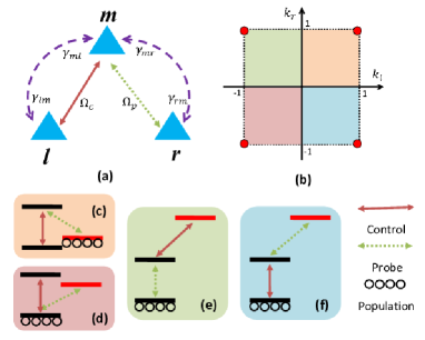
Figure 1: (Color online) (a) Schematic illustration of general three-level system, the levels are denoted by $\left|l\right\rangle$, $\left|r\right\rangle$ and $\left|m\right\rangle$. The coherent and incoherent transitions are denoted by arrows, but the transition between $l$ and $r$ is forbidden. (b) The incoherent transition ratio parameter space of TLS. The four typical categories of energy level structure: $\Lambda$-TLS (c), $V$-TLS (d), upper-level-driving $\Xi$-TLS (e) and lower-level-driving $\Xi$-TLS (f), which are corresponding to the four vertexes (red dots) in (b).

Model.- Shown in Fig. 1(a) is the schematic illustration of generalized TLS, with energy levels denoted by left ($\left|l\right\rangle$), right ($\left|r\right\rangle$) and middle ($\left|m\right\rangle$). The transition between $l$ and $r$ is forbidden, and there are control and probe lasers excite the transitions $l-m$ and $m-r$ near-resonantly. Due to the symmetry, we denote the $l-m$ transition as control laser and the $m-r$ transition as probe without loss of generality. The kernel of the unified framework of TLS is that the incoherent transitions $l-m$, $m-l$, $r-m$ and $m-r$ are all taken into consideration. These incoherent transitions mainly due to the spontaneous emission relaxation process and incoherent pumping. It is well known that the atomic spontaneous emission rate can be inhibited and accelerated by changing the electromagnetic density of states due to thew Purcell effect Scully1997 , thus the relaxation rate can be controlled in experiment. The incoherent pumping can be realized by incoherent light source or pumping electrons to energy levels outside the TLS, and incoherent transition rate can be adjusted simply by changing the pumping power.

By controlling the incoherent transition rate, the steady state populations of TLS without external coherent driving at thermal equilibrium can be arbitrary mixing of the three levels. Denote the incoherent transition rate from level $a$ to level $b$ as $\gamma_{ba}$, and introduce the transition ratios

$$k_{l} = \frac{\gamma_{lm}-\gamma_{ml}}{\gamma_{lm}+\gamma_{ml}},$$ (1)

$$k_{r} = \frac{\gamma_{rm}-\gamma_{mr}}{\gamma_{rm}+\gamma_{mr}}.$$ (2)

Thus, we can have steady state populations equivalent to four typical energy level structures [as shown in Fig. 1(c)-(f)]: (i) lower-level-driving $\Xi$-TLS with $k_{l}=1$ and $k_{r}=-1$; (ii) upper-level-driving $\Xi$-TLS with $k_{l}=-1$ and $k_{r}=1$, (iii) $V$-TLS with $k_{l}=-1$ and $k_{r}=-1$, (iv) $\Lambda$-TLS with $k_{l}=1$ and $k_{r}=1$. Previous studies on the coherent light-TLS interactions are focused on these four specific atomic energy level structures, and found that EIT can only be observed in $\Lambda$- [Fig. 1(c)] and upper-level-driving $\Xi$- [Fig. 1(e)] TLSs RevModPhys.77.633 . In the parameter space $k_{l},\ k_{r}\in[-1,\ 1]$, the well-studied four typical energy level structures are corresponding to the vertexes in Fig. 1(b). Interesting physical phenomena can be observed in the intermediate parameter region by tuning the incoherent control parameters. For example, increase $\gamma_{lm}$ monotonously, the effective energy level structures are transformed continuously from $\Lambda$-TLS to $\Xi$-TLS. Therefore, the EIT or ATS spectrum can be observed in arbitrary TLS by incoherent control.

Hamiltonian and solutions.- The Hamiltonian describing the generalized TLS [Fig. 1(a)] is $H=-\Delta_{c}\left|l\right\rangle\left\langle l\right|-\Delta_{p}\left|r\right\rangle\left\langle r\right|+\frac{1}{2}(\Omega_{c}\left|m\right\rangle\left\langle l\right|+\Omega_{p}\left|m\right\rangle\left\langle r\right|+h.c.)$ with control and probe laser detuning $\Delta_{c}$ and $\Delta_{p}$, coupling strength $\Omega_{c}$ and $\Omega_{p}$. The dynamics of the system is governed by the Master equation Scully1997 , which reads

$$\frac{d}{dt}\rho= -i[H,\rho]+\sum_{x=l,m,r}\gamma_{xx}\mathscr{L}(\left|x\right\rangle\left\langle x\right|)\rho$$

$$+\sum_{x=l,r}\left[\gamma_{mx}\mathscr{L}(\left|m\right\rangle\left\langle x\right|)\rho+\gamma_{xm}\mathscr{L}(\left|x\right\rangle\left\langle m\right|)\rho\right],$$ (3)

with the Lindblad super-operator $\mathscr{L}(o)\rho=o\rho o^{\dagger}-\frac{1}{2}\rho o^{\dagger}o-\frac{1}{2}o^{\dagger}o\rho$. The parameter $\gamma_{xx}$ denotes the dephasing of $\left|x\right\rangle$ ($x=l,m,r$). The steady state solution of the Master equation to zeroth order perturbation of $\Omega_{p}$ is $\rho_{mm}=\frac{-\gamma_{mr}\left(A-\gamma_{ml}\right)}{-A\left(2\gamma_{mr}+\gamma_{rm}\right)+\gamma_{ml}\left(\gamma_{mr}+\gamma_{rm}\right)+\gamma_{mr}\gamma_{lm}}$, where $A=\frac{\left|\Omega_{c}\right|^{2}}{2}\mathrm{Re}[\frac{1}{i\Delta_{c}-(\gamma_{ml}+\gamma_{lm}+\gamma_{rm}+\gamma_{ll}+\gamma_{mm})/2}]$. To the first order of $\Omega_{p}$, the density matrix element $\rho_{mr}=\frac{\Omega_{p}}{2}\chi$, where the susceptibility of the probe laser can be written as

$$\chi=\frac{iC\left(i\Delta_{p}+D\right)}{\omega_{mr}\omega_{lr}+\frac{\left|\Omega_{c}\right|^{2}}{4}}.$$ (4)

Here, $C=\frac{\gamma_{rm}-\gamma_{mr}}{\gamma_{mr}}\rho_{mm}$, $D=\frac{\gamma_{ml}+\gamma_{mr}+\gamma_{ll}+\gamma_{rr}}{2}-\frac{\left|\Omega_{c}\right|^{2}}{4\omega_{lm}}\frac{\gamma_{mr}-\left(2\gamma_{mr}+\gamma_{rm}\right)\rho_{mm}}{\left(\gamma_{rm}-\gamma_{mr}\right)\rho_{mm}}$, $\omega_{lr}=-i(\Delta_{p}-\Delta_{c})-\frac{\gamma_{ml}+\gamma_{mr}+\gamma_{ll}+\gamma_{rr}}{2}$ and $\omega_{mr}=-i\Delta_{p}-\frac{\gamma_{lm}+\gamma_{mr}+\gamma_{rm}+\gamma_{mm}+\gamma_{rr}}{2}$. Obviously, $C$ and $D$ are real numbers, and the denominator in Eq. 4 can be written in the form as $\omega_{mr}\omega_{lr}+\frac{\left|\Omega_{c}\right|^{2}}{4}=\left(i\Delta_{p}+\delta_{1}\right)\left(i\Delta_{p}+\delta_{2}\right)$ with $\delta_{1,2}=\gamma_{s}\pm\frac{\sqrt{\Omega_{s}^{2}-|\Omega_{c}|^{2}}}{2}$. Here $\gamma_{s}=\frac{\gamma_{ml}+2\gamma_{mr}+\gamma_{lm}+\gamma_{rm}+\gamma_{mm}+\gamma_{ll}+2\gamma_{rr}}{4}$, and

$$\Omega_{s}=|\frac{\gamma_{lm}+\gamma_{rm}+\gamma_{mm}-\gamma_{ml}-\gamma_{ll}}{2}|$$ (5)

is the critical control strength.

When $|\Omega_{c}|=\Omega_{s}$, which means that $\delta_{1}=\delta_{2}$, we have

$$\chi=\frac{iC\left(i\Delta_{p}+D\right)}{\left(i\Delta_{p}+\delta_{1}\right)^{2}}.$$ (6)

When $\delta_{1}\neq\delta_{2}$, the susceptibility is composed by two resonances

$$\chi=\frac{iC}{\delta_{2}-\delta_{1}}(\frac{D-\delta_{1}}{i\Delta_{p}+\delta_{1}}-\frac{D-\delta_{2}}{i\Delta_{p}+\delta_{2}}).$$ (7)

From the view of resonance interference, the TLS in control laser field can be divided to two regimes: (a) degenerate regime ($\left|\Omega_{c}\right|<\Omega_{s}$), (b) non-degenerate regime ($\left|\Omega_{c}\right|>\Omega_{s}$). For the sake of the simplicity and clarity of the results, we set the control laser detuning $\Delta_{c}=0$. In the following, we are focus on the incoherent control by adjusting $\gamma_{mr}$. Similar phenomena can be expected by adjusting other parameters, since the essential underlying physics is the same.

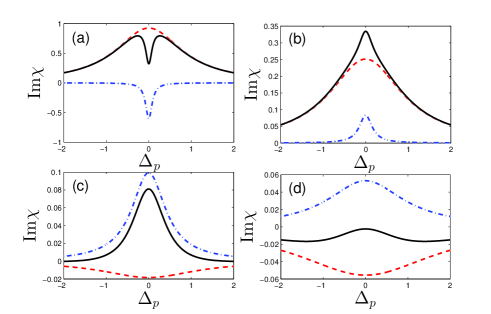
Figure 2: In the degenerate regime, $\mathrm{Im}\chi$ as a function of the probe laser detuning $\Delta_{p}$ with the increasing of $\gamma_{mr}$. Each subplot includes the first resonance $\chi_{1}$ (the red dashed line), second resonance $\chi_{2}$ (the blue dash-dotted line), and the total $\mathrm{Im}\chi$ (the black solid line). (a)-(d) The incoherent transition rates are $\gamma_{mr}=0.02$, $0.2$, $0.8$ and $2$, with fixed $\Omega_{c}=0.5$. Other parameters are $\gamma_{ml}=0.01$, $\gamma_{lm}=1$, $\gamma_{rm}=1$, $\gamma_{ll}=0.01$, $\gamma_{mm}=0.01$, and $\gamma_{rr}=0.01$.

Degenerate Regime.- When the control light is weak $\left(\left|\Omega_{c}\right|<\Omega_{s}\right)$, the two resonances are degenerated but with different linewidth $\delta_{1}$ and $\delta_{2}$ $\left(\delta_{1}>\delta_{2}\right)$. Then we can obtain the imaginary part of linear susceptibility (proportional to the absorption coefficient)

$$\mathrm{Im}(\chi)=\chi_{1}+\chi_{2},$$ (8)

as an overlap of two resonances ($k=1,2$) with

$$\chi_{k}=\frac{C(D-\delta_{k})}{(-1)^{k}(\delta_{1}-\delta_{2})}\mathrm{Re}\left(\frac{1}{i\Delta_{p}+\delta_{k}}\right).$$ (9)

In the degenerate regime, it is possible to suppress the absorption through the cancellation of two resonances. We plot $\mathrm{Im}(\chi)$ as a function of the probe laser detuning $\Delta_{p}$ with the increasing of the incoherent transition rate $\gamma_{mr}$ in the Fig. 2. Each subplot includes the first resonance $\chi_{1}$ (the red dashed line), second resonance $\chi_{2}$ (the blue dash-dotted line), and $\mathrm{Im}\chi$ (the black solid line), which clearly show the relation between the two resonances and the total absorption. From the parameters, we obtain the critical control strength $\Omega_{s}=0.995$, and the $\Omega_{c}<\Omega_{s}$ is satisfied. In the Fig. 2(a), we set $\gamma_{mr}=0.02$, and the EIT phenomenon is observed with a very sharp dip in the total absorption spectrum. We have $C>0,$ $D<\delta_{2}$ and $\delta_{2}\ll\delta_{1},$ and it means that the narrow dip from the second resonance is added to the first resonance with the wide absorption peak, which is observed from the resonance $\chi_{1}$ and $\chi_{2}$. Fig. 2(b) shows that the absorption is enhanced with $\gamma_{mr}=0.2$, and now we have $C>0$ and $\delta_{2}<D<\delta_{1}$. Obviously the amplitude of the two resonances are with the same sign, which leads to a sharp peak of total absorption and is known as electromagnetic induced absorption (EIA). With increasing $\gamma_{mr}$, we have $D>\delta_{1}$, and the amplitude becomes negative from the $\chi_{1}$ in the Fig. 2(c). The strength of the first resonance is weaker compared to the second resonance, and the total absorption spectrum is only weakened. When we set $\gamma_{mr}=2>\gamma_{rm}$, which means $C<0$, then we have $D<\delta_{2}$. We observe the EIT in the amplification spectrum from the Fig. 2(d), which means that the amplification of probe light is suppressed by the control laser. From above results, we can only expect the EIT or EIA in the degenerate regime. It’s worth noting that $\Omega_{s}=0$ when $\gamma_{lm}+\gamma_{rm}+\gamma_{mm}-\gamma_{ml}-\gamma_{ll}=0$, which means there is no degenerate regime.

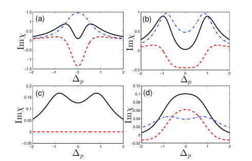
Figure 3: In the non-degenerate regime, $\mathrm{Im}\chi$ as a function of the probe laser detuning $\Delta_{p}$ with the different $\gamma_{mr}$ and $\Omega_{c}$. Each subplot includes $\mathrm{Im}(\chi_{E})$ (the red dashed line), $\mathrm{Re}(\chi_{A})$ (the blue dash-dotted line), and the total $\mathrm{Im}\chi$ (the black solid line). (a) $\Omega_{c}=1.1$, $\gamma_{mr}=0.02$ . (b) $\Omega_{c}=2$, $\gamma_{mr}=0.02$ .(c) $\Omega_{c}=2$, $\gamma_{mr}=0.5025$ .(d) $\Omega_{c}=2$, $\gamma_{mr}=0.8$ . The remaining parameters are the same as Fig. 2.

Non-degenerate Regime.- When pump laser is strong that $\left|\Omega_{c}\right|>\Omega_{s}$, the frequency splitting between two resonances is given by

$$\triangle_{s}=\sqrt{\left|\Omega_{c}\right|^{2}-\Omega_{s}^{2}},$$ (10)

and the linewidth of two resonances are equal to $\gamma_{s}$. The expression of susceptibility is significantly different from the degenerate regime, where the coefficients of two resonances are both real numbers. The imaginary part of linear susceptibility for splitting regime can be written as

$$\mathrm{Im}(\chi)=\mathrm{Im}(\chi_{E})+\mathrm{Re}(\chi_{A}),$$ (11)

where $\chi_{E}=-\frac{C(D-\gamma_{s})}{\triangle_{s}}\left(\frac{1}{\omega_{+}}-\frac{1}{\omega_{-}}\right),\ \chi_{A}=\frac{C}{2}\left(\frac{1}{\omega_{+}}+\frac{1}{\omega_{-}}\right).$and $\omega_{\pm}=i\left(\Delta_{p}\pm\frac{1}{2}\triangle_{s}\right)+\gamma_{s}$.

Fig. 3 is a set of $\mathrm{Im}(\chi)$ as a function of the probe laser detuning $\Delta_{p}$ with the different incoherent transition rate $\gamma_{mr}$ and the control light $\Omega_{c}$ in the condition $\left|\Omega_{c}\right|>\Omega_{s}$. The red dashed line represents $\mathrm{Im}(\chi_{E})$, which is related to the EIT as interaction, the blue dash-dotted line $\mathrm{Re}(\chi_{A})$ is the sum of two Lorentzian peaks, corresponding to the ATS, and the black solid line is the total spectrum $\mathrm{Im}(\chi)$. In Fig. 3(a), we choose the parameters with $D\ll\gamma_{s}$, $\Delta_{s}<\gamma_{s}$. In this case, the splitting of two Lorentzian peaks is smaller than the linewidth, and the dip is only from the $\mathrm{Im}(\chi_{E})$. The condition $\Delta_{s}>\gamma_{s}$ is observed in the Fig. 3(b) with increasing of $\Omega_{c}$, and we can see two peaks from the blue dash-dotted line, which reflects the cross-over from EIT to ATS. If we tune the incoherent transition rate $\gamma_{mr}$ to satisfy $D=\gamma_{s}$, $\chi_{E}$ is zero as shown in Fig. 3(c), and the spectrum becomes ATS consisting of two Lorentzian shaped peaks. When $D>\gamma_{s}$, as plotted in Fig. 3(d), the transparency from the splitting of two Lorentz peaks is hided because of the $\mathrm{Im}(\chi_{E})$. From the Fig. 3, we can realize the cross-over from EIT to ATS by adjusting incoherent transition rate $\gamma_{mr}$ and the control light $\Omega_{c}$.

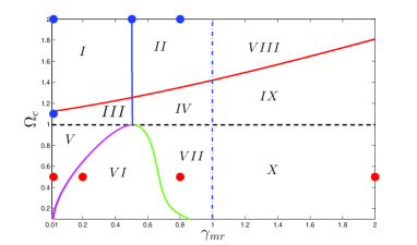
Figure 4: The black dashed line : $|\Omega_{c}|=\Omega_{s}$, the blue dash-dotted line : $C=0$ $\left(\gamma_{mr}=\gamma_{rm}=1\right)$, the blue line : $D=\gamma_{s},$ the red line: $\Delta_{s}=\gamma_{s},$ the magenta line: $D=\delta_{2},$ the green line: $D=\delta_{1},$ and the red and blue dots correspond to Fig. 2 and 3, respectively. The remaining parameters are the same as Fig. 2.

Phase Diagram.- To intuitively understand different lineshapes and the crossover between EIT and ATS, we plot the phase diagram in the Fig. 4 by controlling incoherent transition rate $\gamma_{mr}$ and the control light $\Omega_{c}$. The black dashed line is critical condition for splitting $|\Omega_{c}|=\Omega_{s}$, which shows spectrum from the Eq. 6. The blue dash-dotted line shows $C=0$ $\left(\gamma_{mr}=\gamma_{rm}=1\right)$, and for the regions with incoherent transition rate $\gamma_{mr}<\gamma_{rm}\ (\gamma_{mr}>\gamma_{rm})$, we have $C>0\ (C<0)$. The red and blue dots denotes parameters of Fig. 2 and 3, respectivly. Below the black dashed line is the degenerate regime with $|\Omega_{c}|<\Omega_{s}$, and the magenta and green lines indicate $D=\delta_{2}$ and $D=\delta_{1}$, respectively. In the zone $V$, the two resonances are out of phase, which leads to the EIT shown in the Fig. 2(a). In contrast, the two resonances are in phase in the zone $VI$, and the spectrum shows EIA, as shown in the Fig. 2(b). The zone $VII$ and $X$ corresponds to $C>0,$ $D>\delta_{1}$ and $C<0,$ $D<\delta_{2}$, respectively, and the two resonances are always out of phase. The typical spectra in zones $VII$ and $X$ are Fig. 2(c) and (d) with $C>0$ and $C<0$, respectively.

In the non-degenerate regime (upon the black dashed line), there are six zones divided by the blue line, red line and the blue dash-dotted line, and all blue dots satisfy $C>0$. The blue line represents $D=\gamma_{s},$ in which case the coefficient of $\chi_{E}$ vanishes and the spectrum is the sum of two Lorentzian peaks [Fig. 3(c)]. The red line corresponds to $\Delta_{s}=\gamma_{s}$, indicating that the splitting between the two resonances equals the linewidth. In the zone $I$, we have $D<\gamma_{s},$ $\varDelta_{s}>\gamma_{s},$ the destructive interference between the ATS and EIT components leads to enhanced transparency window, as shown in Fig. 3(b). When $D>\gamma_{s},$ $\varDelta_{s}>\gamma_{s},$ it is the zone $II$, the transparency window of two Lorentz peaks is weakened due to the constructive interference between ATS and EIT, as shown in Fig. 3(d). In the zone $III$, with the typical spectrum shown in Fig. 3(a), the splitting between two Lorentz peaks is smaller than the linewidth. The lineshape shows a transparency window from EIT in Fig. 2(a) to the spectrum in Fig. 3(a, b), which illustrates the crossover from zones $V$ to $I$ via zone $III$. The zone $IV$ means the incoherent transition rate $\gamma_{mr}$ becomes larger compared to the control light $\Omega_{c}$, then the electromagnetically induced transparency with respect to the amplification should be realized, and the zones $VIII$ and $IX$ are opposite to the zones $II$ and $IV$, respectively, with $C<0$.

Conclusion.- The dispersion and absorption of probe light in the three-level system is studied with the coherent laser driving and incoherent control. In the degenerate regime, EIT in respect to absorption or amplification is due to the interference of two resonances with different linewidths. In the non-degenerate regime, the cross-over from EIT to ATS is possible by increasing the driving power or controlling the incoherent transition rates. By varying both coherent and incoherent parameters of the three-level system, rich quantum phenomena of light-matter interaction can be exemplified.

Acknowledgments. This work was funded by National Natural Science Foundation of China (11074244 and 11274295), 973project (2011cba00200). LJ acknowledges support from the Alfred P Sloan Foundation, the Packard Foundation, the AFOSR-MURI, the ARO, and the DARPA Quiness program.

References

- (1) M. O. Scully and M. S. Zubairy, Quantum Optics (Cambridge University Press, 1997).
- (2) K.-J. Boller, A. Imamolu, and S. Harris, Phys. Rev. Lett. 66, 2593 (1991).
- (3) S. E. Harris, Phys. Today 50, 36 (1997).
- (4) M. D. Lukin and A. Imamoglu, Nature 413, 273 (2001).
- (5) M. Lukin, Rev. Mod. Phys. 75, 457 (2003).
- (6) M. Fleischhauer, A. Imamoglu, and J. P. Marangos, Rev. Mod. Phys. 77, 633 (2005).
- (7) M. Phillips, H. Wang, I. Rumyantsev, N. Kwong, R. Takayama, and R. Binder, Phys. Rev. Lett. 91, 183602 (2003).
- (8) Q. Xu, S. Sandhu, M. Povinelli, J. Shakya, S. Fan, and M. Lipson, Phys. Rev. Lett. 96, 123901 (2006).
- (9) N. Liu, L. Langguth, T. Weiss, J. Kästel, M. Fleischhauer, T. Pfau, and H. Giessen, Nat. Mater. 8, 758 (2009).
- (10) N. Papasimakis, V. Fedotov, N. Zheludev, and S. Prosvirnin, Phys. Rev. Lett. 101, 253903 (2008).
- (11) S. Weis, R. Rivière, S. Deléglise, E. Gavartin, O. Arcizet, A. Schliesser, and T. J. Kippenberg, Science 330, 1520 (2010).
- (12) N. Liu et al., Nano Lett. 10, 1103 (2010).
- (13) B. Luk’yanchuk et al., Nat. Mater. 9, 707 (2010).
- (14) M. Albert, A. Dantan, and M. Drewsen, Nat. Photonics 5, 633 (2011).
- (15) P. M. Anisimov, J. P. Dowling, and B. C. Sanders, Phys. Rev. Lett. 107, 163604 (2011).
- (16) T. Y. Abi-Salloum, Phys. Rev. A 81, 053836 (2010).
- (17) C. Zhu, C. Tan, and G. Huang, Phys. Rev. A 87, 043813 (2013).
- (18) L. Giner et al., Phys. Rev. A 87, 013823 (2013).
- (19) T. Oishi, R. Suzuki, A.I. Talukder, and M. Tomita, Phys. Rev. A 88, 023847 (2013).
- (20) B. Peng, S. Ozdemir, and W. Chen, arXiv 1404.5941 (2014).