Performance Engineering of the Kernel Polynomial Method on Large-Scale CPU-GPU Systems

Abstract

The Kernel Polynomial Method (KPM) is a well-established scheme in quantum physics and quantum chemistry to determine the eigenvalue density and spectral properties of large sparse matrices. In this work we demonstrate the high optimization potential and feasibility of peta-scale heterogeneous CPU-GPU implementations of the KPM. At the node level we show that it is possible to decouple the sparse matrix problem posed by KPM from main memory bandwidth both on CPU and GPU. To alleviate the effects of scattered data access we combine loosely coupled outer iterations with tightly coupled block sparse matrix multiple vector operations, which enables pure data streaming. All optimizations are guided by a performance analysis and modelling process that indicates how the computational bottlenecks change with each optimization step. Finally we use the optimized node-level KPM with a hybrid-parallel framework to perform large scale heterogeneous electronic structure calculations for novel topological materials on a petascale-class Cray XC30 system.

It is widely accepted that future supercomputer architectures will change considerably compared to the machines used at present for large scale simulations. Extreme parallelism, use of heterogeneous compute devices and a steady decrease in the architectural balance in terms of main memory bandwidth vs. peak performance are important factors to consider when developing and implementing sustainable code structures. Accelerator-based systems already account for a performance share of 34% of the total TOP500 [1] today, and they may provide first blueprints of future architectural developments. The heterogeneous hardware structure typically calls for a completely new software development, in particular if the simultaneous use of all compute devices is addressed to maximize performance and energy efficiency.

A prominent example demonstrating the need for new software implementations and structures is the MAGMA project [2]. In dense linear algebra the code balance (bytes/flop) of basic operations can often be reduced by blocking techniques to better match the machine balance. Thus, this community is expected to achieve high absolute performance also on future supercomputers. In contrast, sparse linear algebra is known for low sustained performance on state of the art homogeneous systems. The sparse matrix vector multiplication (SpMV) is often the performance-critical step. Most of the broad research on optimal SpMV data structures has been devoted to drive the balance of a general SpMV (not using any special matrix properties) down to its minimum value of $6\,\mbox{bytes}/\mbox{flop}$ (double precision) or $2.5\,\mbox{bytes}/\mbox{flop}$ (double complex) on all architectures, which is still at least an order of magnitude away from current machine balance numbers. Just recently the long known idea of applying the sparse matrix to multiple vectors at the same time (SpMMV) (see, e.g., [3]), to reduce computational balance has gained new interest [4, 5].

A representative of the numerical sparse linear algebra schemes used in applications that can benefit from SpMMV is the Kernel Polynomial Method (KPM). KPM was originally devised for the computation of eigenvalue densities and spectral functions [6], and soon found applications throughout physics and chemistry (see [7] for a review). KPM can be broadly classified as a polynomial-based expansion scheme, with the corresponding simple iterative structure of the basic algorithm that addresses the large sparse matrix from the application exclusively through SpMVs. Recent applications of KPM include, e.g., eigenvalue counting for predetermination of sub-space sizes in projection-based eigensolvers [8] or for large scale data analysis [9].

In this paper we present for the first time a structured performance engineering process for the KPM that substantially brings down the computational balance of the method, leading to high sustained performance on CPUs and GPUs. The algorithm itself is untouched; all optimizations are strictly changes to the implementations. We apply a data-parallel approach for combined CPU-GPU parallelization and present the first large-scale heterogeneous CPU-GPU computations for KPM. The main contributions of our work which are of broad interest beyond the original KPM community are as follows:

We achieve a systematic reduction of code balance for a widely used sparse linear algebra scheme by implementing a tailored, algorithm-specific (“augmented”) SpMV routine instead of relying on a series of sparse linear algebra routines taken from an optimized general library like BLAS. We reformulate the algorithm to use SpMMV in order to combine loosely coupled outer iterations. Our systematic performance analysis for the SpMMV operation on both CPU and GPU indicates that SpMMV decouples from main memory bandwidth for sufficiently large vector blocks, and that data cache access then becomes a major bottleneck on both architectures. Finally we demonstrate the feasibility of large-scale CPU-GPU KPM computations for a technologically highly relevant application scenario, namely topological materials. In our experiments, the augmented SpMMV KPM version achieves more than $100\,\mbox{Tflop/s}$ on 1024 nodes of a CRAY XC30 system. This is equivalent to almost 10% of the aggregated CPU-GPU peak performance.

An open-source program library containing all presented software developments as well as the KPM application code are available for download [10].

-A Related Work

SpMV has been – and still is – a highly active subject of research due to the relevance of this operation in applications of computational science and engineering. It has turned out that the sparse matrix storage format is a critical factor for SpMV performance. Fundamental research on sparse matrix formats for the architectures considered in this work has been conducted by Barrett et al. [11] for cache-based CPUs and Bell et al. [12] for GPUs. The assumption that efficient sparse matrix storage formats are dependent on and exclusive to a specific architecture has been refuted by Kreutzer et al. [13] by showing that a unified format (SELL-C-$\sigma$) can yield high performance on both architectures under consideration in this work. Vuduc [14] provides a comprehensive overview of optimization techniques for SpMV.

Early research on performance bounds for SpMV and SpMMV has been done by Gropp et al. [3] who established a performance limit taking into account both memory- and instruction-boundedness. A similar approach has been pursued by Liu et al. [4], who established a finer yet similar performance model for SpMMV. Further refinements to this model have been accomplished by Aktulga et al. [5], who not only considered memory- and instruction-boundedness but also bandwidth bounds of two different cache levels.

On the GPU side, literature about SpMMV is scarce. The authors of  [12] mention the potential performance benefits of SpMMV over SpMV in the outlook of their work. Anzt et al. [15] have recently presented a GPU implementation of SpMMV together with performance and energy results. The fact that SpMMV is implemented in the library cuSPARSE [16], which is shipped together with the CUDA toolkit, proves the relevance of this operation.

Optimal usage patterns for heterogeneous supercomputers have become an increasingly important topic with the emergence of those architectures. An important attempt towards high performance heterogeneous execution is MAGMA [2]. However, the hybrid functions delivered by this toolkit are restricted to dense linear algebra. Furthermore, MAGMA employs task-based work distribution, in contrast to the symmetric data-parallel approach used in this work. Matam et al. [17] have implemented a hybrid CPU/GPU solver for sparse matrix-multiplication. However, they do not scale their solution beyond a single node.

Zhang et al. [18] have presented a KPM implementation for a single NVIDIA GPU, but they do not follow the conventional data-parallel approach. Memory footprint and corresponding main memory access volume of their implementation scale linearly with the number of active CUDA blocks, which limits applicability and performance severely.

-B Application Scenario: Topological Materials

To support our performance analysis with benchmark data from a real application we will apply our improved KPM implementation to a problem of current interest, the determination of electronic structure properties of a three-dimensional (3D) topological insulator.

Topological insulators form a novel material class similar to graphene with promising applications in fundamental research and technology [19]. The hallmark of these materials is the existence of topologically conserved quantum numbers, which are related to the familiar winding number from two-dimensional geometry, or to the Chern number of the integer quantum Hall effect. The existence of such strongly conserved quantities makes topological materials first-class candidates for quantum computing and quantum information applications.

The theoretical modelling of a typical topological insulator is specified by the Hamilton operator

$$\begin{split}H=-t\sum_{\begin{subarray}{c}j=1,2,3\\[0.60275pt] n\end{subarray}}\left(\Psi_{n+\hat{\text{e}}_{j}}^{\dagger}\frac{\Gamma^{1}-\text{i}\Gamma^{j+1}}{2}\Psi_{n}+\text{H.c.}\right)\\ +\sum_{n}\Psi_{n}^{\dagger}\left(V_{n}\Gamma^{0}+2\Gamma^{1}\right){\Psi_{n}}\;,\end{split}$$ (1)

which describes the quantum-mechanical behavior of an electric charge in the material, subject to an external electric potential $V_{n}$ that is used to create a superlattice structure of quantum dots. The vector space underlying this operator can be understood as the product of a local orbital and spin degree of freedom, which is associated with the $4\times 4$ Dirac matrices $\Gamma^{a}$, and the positional degree of freedom $n$ on the 3D crystalline structure composing the topological insulator. We cite the Hamilton operator for the sake of completeness although its precise form is not relevant for the following investigation. For further details see, e.g., Refs. [20, 21].

From the expression (1) one obtains the sparse matrix representation of the Hamilton operator by choosing appropriate boundary conditions and spelling out the entries of the matrices $\Gamma^{a}$. Here, we treat finite $N_{x}\times N_{y}\times N_{z}$ samples, such that the matrix $H$ in the KPM algorithm has dimension $N=4N_{x}\times N_{y}\times N_{z}$. The matrix is complex and Hermitian, the number of non-zero entries is $N_{\mathrm{nz}}\approx 13N$.

Characteristic for these applications is the presence of several sub-diagonals in the matrix. Periodic boundary conditions in the $x$ and $y$ directions lead to outlying diagonals in the matrix corners. In the present example, the matrix is a stencil but not a band matrix. Because of the quantum dot superlattice structure, translational symmetry is not available to reduce the problem size. This makes the current problem relevant for large-scale computations.

One basic quantity of interest for physics applications is the eigenvalue density, or density of states (DOS),

$$\rho(E)=\sum_{n=1}^{N}\delta(E-E_{n})=\mathrm{tr}[\delta(E\mathbb{1}-H)]\;,$$ (2)

where the sum of the trace $\mathrm{tr}[\dots]$ runs over all eigenvalues $E_{n}$ of $H$. The DOS quantifies the number of eigenvalues per interval, and can also be used, e.g., to predict the required size of sub-spaces for eigenvalue projection techniques [8, 22].

A direct method for computation of $\rho(E)$ that uses the first expression in (2) would have to determine all eigenvalues of $H$, which is not feasible for large matrices. Instead, we rely on the KPM-DOS algorithm introduced in the next section. In Figs. 1, 2 a few data for the DOS obtained with KPM-DOS are shown for the present application.

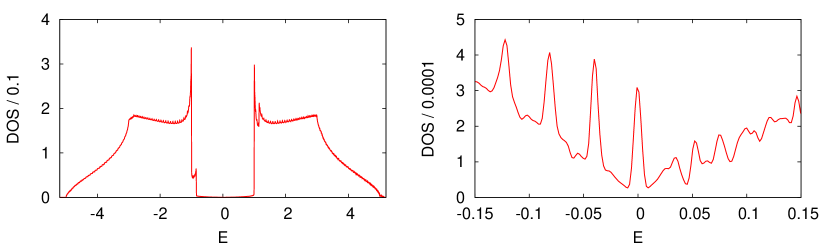
Figure 1: DOS for a $1600\times 1600\times 40$ topological insulator ($N\approx 4\times 10^{8}$) computed with the KPM-DOS algorithm.

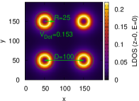
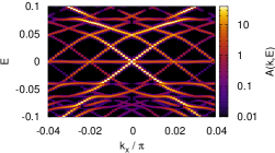
Figure 2: Left panel: Local DOS for a quantum dot superlattice imposed on top of a topological insulator. Right panel: Corresponding momentum-resolved spectral function $A(k,E)$. See, e.g., Refs. [20, 21] for details on the physics.

I Problem Description

The KPM is a polynomial expansion technique for the computation of spectral quantities of large sparse matrices (see our review [7] for a detailed exposition). In the context of the definition (2) the KPM does not work directly with the first expression, but with a systematic expansion of the $\delta$-function in the second expression. KPM is based on the orthogonality properties and two-term recurrence for Chebyshev polynomials $T_{m}(x)$ of the first kind. Specifically, in KPM one successively computes the vectors $|\nu_{m}\rangle=T_{m}(\tilde{H})|\nu_{0}\rangle$ from a starting vector $|\nu_{0}\rangle$, for $1\leq m\leq M/2$ with prescribed $M$, through the recurrence

$$|\nu_{1}\rangle=\tilde{H}|\nu_{0}\rangle\;,\quad|\nu_{m+1}\rangle=2\tilde{H}|\nu_{m}\rangle-|\nu_{m-1}\rangle\;.$$ (3)

The recurrence involves the matrix $\tilde{H}$ only in (sparse) matrix-vector multiplications. Note that one must re-scale the original matrix as $\tilde{H}=a(H-b\mathbb{1})$ such that the spectrum of $\tilde{H}$ is contained in the interval of orthogonality $[-1,1]$ of the Chebyshev polynomials. Suitable values $a,b\in\mathbb{R}$ are determined initially with Gershgorin’s circle theorem or a few Lanczos sweeps.

From the vectors $|\nu_{m}\rangle$ two scalar products $\eta_{2m}=\langle\nu_{m}|\nu_{m}\rangle$, $\eta_{2m+1}=\langle\nu_{m+1}|\nu_{m}\rangle$ are computed in each iteration step. Spectral quantities are reconstructed from these scalar products in a second computationally inexpensive step, which is independent of the KPM iteration and needs not be discussed in the context of performance engineering. For the computation of a spectrally averaged quantity, e.g., the DOS from Eq. (2), the trace can be approximated by a sum over several independent random initial vectors as in $\mathrm{tr}[A]\approx(1/R)\sum_{r=1}^{R}\langle\nu^{(r)}_{0}|A|\nu^{(r)}_{0}\rangle$ (see [7] for further details).

for  $r=0$ to $R-1$  do

     $|v\rangle\leftarrow|\mbox{rand()}\rangle$

     Initialization steps and computation of $\eta_{0},\eta_{1}$

     for  $m=1$ to $M/2$  do

         $\mbox{swap}(|w\rangle,|v\rangle)$

         $\mathrlap{|u\rangle}\phantom{\eta_{2m+1}}\leftarrow H|v\rangle$ $\triangleright$ spmv()

         $\mathrlap{|u\rangle}\phantom{\eta_{2m+1}}\leftarrow|u\rangle-b|v\rangle$ $\triangleright$ axpy()

         $\mathrlap{|w\rangle}\phantom{\eta_{2m+1}}\leftarrow-|w\rangle$ $\triangleright$ scal()

         $\mathrlap{|w\rangle}\phantom{\eta_{2m+1}}\leftarrow|w\rangle+2a|u\rangle$ $\triangleright$ axpy()

         $\mathrlap{\eta_{2m}}\phantom{\eta_{2m+1}}\leftarrow\langle v|v\rangle$ $\triangleright$ nrm2()

         $\eta_{2m+1}\leftarrow\langle w|v\rangle$ $\triangleright$ dot()

     end for

end for

Figure 3: Naive version of the KPM-DOS algorithm with corresponding BLAS level 1 function calls. Note that the “swap” operation is not performed explicitly but merely indicates the logical change of the role of the $v$, $w$ vectors in the odd/even iteration steps.

A direct implementation of the above scheme results in the “naive” version of the KPM-DOS algorithm shown in Fig. 3. One feature of KPM is the very simple implementation of the basic algorithm, which leaves substantial headroom for performance optimization. The above algorithm involves one SpMV and a few BLAS level 1 operations per step. If only two vectors are stored in the implementation the scalar products have to be computed before the next iteration step. That and the multiple individual BLAS level 1 operations on the vectors $|v\rangle,|w\rangle$ call for optimization of the local data access patterns. A careful implementation reduces the amount of global reductions in the dot products to a single one at the end of the inner loop. Furthermore, in its present form the stochastic trace is performed via an outer loop over $R$ random vectors. Although the inner KPM iterations for different initial vectors are independent of each other, performance gains compared to the embarrassingly parallel version with $R$ independent runs can be achieved by incorporating the “trace” functionality into the parallelized algorithm. See Section V-C for detailed performance results.

II Algorithm Analysis and Optimization

To get a first overview of the algorithm’s properties it is necessary to study its requirements in terms of data transfers and computational work, both of which depend on the data types involved. $S_{d}$ and $S_{i}$ denote the size of a single matrix/vector data element and matrix index element, respectively. $F_{a}$ ($F_{m}$) indicates the number of floating point operations (flops) per addition (multiplication).

Funct.	# Calls	Min. Bytes/Call	Flops/Call
spmv()	$RM/2$	$N_{\mathrm{nz}}(S_{d}+S_{i})+$	$N_{\mathrm{nz}}(F_{a}+F_{m})$
		$2NS_{d}$
axpy()	$RM$	$3NS_{d}$	$N(F_{a}+F_{m})$
scal()	$RM/2$	$2NS_{d}$	$NF_{m}$
nrm2()	$RM/2$	$NS_{d}$	$N(\lceil F_{a}/2\rceil+\lceil F_{m}/2\rceil)$
dot()	$RM/2$	$2NS_{d}$	$N(F_{a}+F_{m})$
KPM	1	$RM/2[N_{\mathrm{nz}}(S_{d}+$	$RM/2[N_{\mathrm{nz}}(F_{a}+F_{m})+$
		$S_{i})+13NS_{d}]$	$N(\lceil 7F_{a}/2\rceil+\lceil 9F_{m}/2\rceil)]$

TABLE I: Minimum number of transferred bytes and executed flops for each function involved in Fig. 3.

Table I shows the minimum number of flops to execute and memory bytes to transfer for each of the operations involved in Fig. 3 and for the entire algorithm.

Generally speaking, algorithmic optimization involves a reduction of resource requirements, i.e., lowering either the data traffic or the number of flops. While we assume the latter to be fixed for this algorithm, it is possible to improve on the former. From Fig. 3 it becomes clear that the vectors $u$, $v$, and $w$ are read and written several times. An obvious optimization is to merge all involved operations into a single one. This is a simple and widely applied code optimization technique, also known as loop fusion. In our case, we augment the SpMV kernel with the required operations for shifting and scaling. Furthermore, the needed dot products are being calculated on-the-fly in the same kernel. Note that optimizations of this kind usually require manual implementation due to the lack of libraries providing exactly the kernel as needed. The new kernel will be called aug_spmv() and the resulting algorithm is shown in Fig. 4.

for  $r=0$ to $R-1$  do

     $|v\rangle\leftarrow|\mbox{rand()}\rangle$

     Initialization steps and computation of $\eta_{0},\eta_{1}$

     for  $m=1$ to $M/2$  do

         $\mbox{swap}(|w\rangle,|v\rangle)$

         $|w\rangle=2a(H-b\mathbb{1})|v\rangle-|w\rangle$ &

              $\mathrlap{\eta_{2m}}\phantom{\eta_{2m+1}}=\langle v|v\rangle$ &

              $\eta_{2m+1}=\langle w|v\rangle$ $\triangleright$ aug_spmv()

     end for

end for

Figure 4: Optimization stage 1: Improved version of the KPM-DOS algorithm using the augmented SpMV kernel, which covers all operations chained by ’&’.

The data traffic due to the vectors has been reduced in comparison with the naive implementation in Fig. 3 by saving 10 vector transfers in each inner iteration. A further improvement can be accomplished by exploiting that the same matrix $H-b\mathbb{1}$ gets applied to $R$ different vectors. By interpreting the vectors as a single block vector of width $R$, one can get rid of the outer loop and apply the matrix to the whole block at once. Thus, the resulting operation is an augmented SpMMV, to be referred as aug_spmmv(). The resulting algorithm is shown in Fig. 5.

$\mathrlap{|V\rangle}\phantom{|W\rangle}\vcentcolon=|v\rangle_{0..R-1}$ $\triangleright$ Assemble vector blocks

$|W\rangle\vcentcolon=|w\rangle_{0..R-1}$

$\mathrlap{|V\rangle}\phantom{|W\rangle}\leftarrow|\mbox{rand()}\rangle$

Initialization steps and computation of $\mu_{0},\mu_{1}$

for  $m=1$ to $M/2$  do

     $\mbox{swap}(|W\rangle,|V\rangle)$

     $|W\rangle=2a(H-b\mathbb{1})|V\rangle-|W\rangle$ &

              $\mathrlap{\eta_{2m}\mathtt{[:]}}\phantom{\eta_{2m+1}\mathtt{[\;]}}=\langle V|V\rangle$ &

              $\eta_{2m+1}\mathtt{[:]}=\langle W|V\rangle$ $\triangleright$ aug_spmmv()

end for

Figure 5: Optimization stage 2: Blocked and improved version of the KPM-DOS algorithm using the augmented SpMMV kernel. Now, each $\eta$ is a vector of $R$ column-wise dot products of two block vectors.

Now the matrix only has to be read $M/2$ times and the data traffic is reduced further. We summarize the data transfer savings for each optimization stage by showing the evolution of the entire solver’s minimum data traffic $V_{\mathrm{KPM}}$:

$$V_{\mathrm{KPM}} =RM/2[N_{\mathrm{nz}}(S_{d}+S_{i})+13S_{d}N]$$

$$\Downarrow$$

$$=RM/2[N_{\mathrm{nz}}(S_{d}+S_{i})+3S_{d}N]$$

$$\Downarrow\text{Using \PVerb{aug_spmmv()}}$$

$$=M/2[N_{\mathrm{nz}}(S_{d}+S_{i})+3RS_{d}N].$$ (4)

It will become evident that data transfers are the bottleneck in this application scenario; using the relevant data paths to their full potential is thus the key to best performance. While tasking approaches for shortening the critical path may seem promising for the original formulation of the algorithm (see Fig. 3), the optimized version in Fig. 5 is purely data parallel.

II-A General Performance Considerations

Using $V_{\mathrm{KPM}}$ from Eq. 4 and the number of flops as presented in Table I the minimum code balance of the solver is:

$$B_{\mathrm{min}} =\frac{N_{\mathrm{nz}}(S_{d}+S_{i})+3RS_{d}N}{R[N_{\mathrm{nz}}(F_{a}+F_{m})+N(\lceil 7F_{a}/2\rceil+\lceil 9F_{m}/2\rceil)]}$$

$$=\frac{N_{\mathrm{nzr}}/R(S_{d}+S_{i})+3S_{d}}{N_{\mathrm{nzr}}(F_{a}+F_{m})+(\lceil 7F_{a}/2\rceil+\lceil 9F_{m}/2\rceil)}\;\frac{\mbox{bytes}}{\mbox{flop}}.$$

$N_{\mathrm{nzr}}=N_{\mathrm{nz}}/N$ denotes the average number of entries per row, which is approximately 13 in our test case. As we are using complex double precision floating point numbers for storing the vector and matrix data, one data element requires 16 bytes of storage ($S_{d}=16$), while 4-byte integers are used for indexing within the kernels ($S_{i}=4$). Note that the code as a whole uses mixed integer sizes, as 8-byte indices are required for global quantities in large-scale runs. Furthermore, for complex arithmetic it holds that $F_{a}=2$ and $F_{m}=6$. Using the actual values for the test problem, we arrive at

$$B_{\mathrm{min}}(R) =\frac{13/R(16+4)+3\cdot 16}{13(2+6)+(\lceil 7\cdot 2/2\rceil+\lceil 9\cdot 6/2\rceil)}\;\frac{\mbox{bytes}}{\mbox{flop}}$$

$$=\frac{260/R+48}{138}\;\frac{\mbox{bytes}}{\mbox{flop}}$$ (5)

$$B_{\mathrm{min}}(1) \approx 2.23\;\frac{\mbox{bytes}}{\mbox{flop}}$$ (6)

$$\lim_{R\to\infty}B_{\mathrm{min}} \approx 0.35\;\frac{\mbox{bytes}}{\mbox{flop}}$$ (7)

Usually the actual code balance is larger than $B_{\mathrm{min}}$. This is mostly due to part of the SpM(M)V input vector being read from main memory more than once. This can be caused by an unfavorable matrix sparsity pattern or an undersized last level cache (LLC). We quantify the performance impact by a factor $\Omega=V_{\mathrm{meas}}/{V_{\mathrm{KPM}}}$, with $V_{\mathrm{meas}}$ being the actual data transfer volume in bytes as measured with, e.g., LIKWID [23] on CPUs and with NVIDIA’s nvprof  [24] profiling tool on NVIDIA GPUs. Thus, the actual code balance is

$$B=\Omega B_{\mathrm{min}}\;.$$ (8)

Following the ideas of Gropp et al. [3] and Williams et al. [25], a simple roofline model can be constructed. The roofline model assumes that an upper bound for the achievable performance of a loop with code balance $B$ can be predicted as the minimum of the theoretical peak performance $P^{\mathrm{peak}}$ and the performance limit due to the memory bandwidth $b$:

$$P^{*}=\mathrm{min}\left(P^{\mathrm{peak}},\frac{b}{B}\right).$$ (9)

The large code balance for $R=1$ (Eq. 6) indicates that the kernel will be memory-bound in this case on modern standard hardware, i.e., the maximum memory-bound performance according to Eq. 9 is

$$P^{*}_{\mathrm{MEM}}=\frac{b}{B}.$$ (10)

An important observation from Eqs. 6 and 7 is that the code balance decreases when $R$ increases, i.e., when substituting SpMV by SpMMV. In other words, the kernel execution becomes more and more independent from the original bottleneck. On the other hand, larger vector blocks require more space in the cache which may cause an increase of $\Omega$ and, consequently, the code balance. See  [26] for a more detailed analysis of this effect. The application of the roofline model will be discussed in Section IV-A.

III Testbed and Implementation

Table II shows relevant architectural properties of the benchmark systems.

	Clock	SIMD	Cores/	$b$	LLC	$P^{\mathrm{peak}}$
	(MHz)	(Bytes)	SMX	(GB/s)	(MiB)	(Gflop/s)
IVB	2200	32	10	50	25	176
SNB	2600	32	8	48	20	166.4
K20m	706	512	13	150	1.25	1174
K20X	732	512	14	170	1.5	1311

TABLE II: Relevant properties of all architectures used in this paper: Intel Xeon E5-2660 v2 (“IVB”) with fixed clock frequency, Intel Xeon E5-2670 (“SNB”) with turbo mode enabled, NVIDIA Tesla K20m with ECC disabled, and NVIDIA Tesla K20X with ECC enabled

Simultaneous multithreading (SMT) has been enabled on the CPUs, which results in a total thread count of twice the number of cores. Both GPUs implement the “Kepler” architecture where each Streaming Multiprocessor (SMX) features 64 double precision units capable of fused multiply add (FMA). The Intel C Compiler (ICC) version 14 has been used for the CPU code. For the GPU code, the CUDA toolkit 5.5 was employed.

Measurements for the node-level performance analysis (Sections IV-A and IV-B) have been conducted on the Emmy cluster at Erlangen Regional Computing Center (RRZE). This cluster contains a number of nodes combining two IVB CPUs with two K20m GPUs.

For large-scale production runs we used the heterogeneous petascale cluster Piz Daint, a Cray XC30 system located at the Swiss National Computing Centre (CSCS) in Lugano, Switzerland. Each of this system’s 5272 nodes consists of one SNB CPU and one K20X GPU.

III-A General Notes on the Implementation

Although the compute platforms used in this work are heterogeneous at first sight, they have architectural similarities which enable optimization techniques that are beneficial on both architectures. An important property in this regard is data parallelism.

Modern CPUs feature Single Instruction Multiple Data (SIMD) units which enable data-parallel processing on the core level. The current Intel CPUs used here implement the AVX instruction set, which contains 256-bit wide vector registers. Hence, four real or two complex numbers can be processed at once in double precision.

The equivalent hardware feature on GPUs is called Single Instruction Multiple Threads (SIMT), which can be seen as “SIMD on a thread level [27].” Here, a group of threads called warp executes the same instruction at a time. On all modern NVIDIA GPUs a warp consists of 32 threads, regardless of the data type. Instruction divergence within a warp causes serialization of the thread execution. Up to 32 warps are grouped in a thread block, which is the unit of work scheduled on an SMX.

For an efficient utilization of SIMD/SIMT processing the data access has to be contiguous per instruction. On GPUs, load coalescing (i.e., subsequent threads have to access subsequent memory locations) is crucial for efficient global load instructions. Achieving efficient SIMD/SIMT execution for SpMV is connected to several issues like zero fill-in and the need for gathering the input vector data [13]. For SpMV, vectorized access can only be achieved with respect to the matrix data. However, in the case of SpMMV this issue can be solved since contiguous data access is possible across the vectors. Note that it is necessary to store the vectors in an interleaved way (row-major) for best efficiency. If this is not compatible with the data layout of the application, transposing the block vector data may be required. Vectorizing the right-hand side vector data access has the convenient advantage that matrix elements can be accessed in a serial manner, which eliminates the need for any special matrix format. Hence, the CRS format (similar to SELL-1) can be used on both architectures without drawbacks. It is worth noting that CRS/SELL-1 may yield even better SpMMV performance than a SIMD-aware storage format for SpMV like SELL-32, because matrix elements within a row are stored consecutively.

III-B CPU Implementation

The CPU kernels have been hand-vectorized using AVX compiler intrinsics. A custom code generator was used to create fully unrolled versions of the kernel codes for different combinations of the SELL chunk height and the block vector width. As the AVX instruction set supports 32-byte SIMD units, a minimal vector block width of two is already sufficient for achieving perfectly vectorized access to the (complex) vector data.

For memory-bound algorithms (like the naive implementation in Fig. 3) and large working sets, efficient vectorization may not be required for optimal performance. However, as discussed in Section II-A, our optimized kernel is no longer strictly bound to memory bandwidth. Hence, efficient vectorization is a crucial ingredient for high performance. To guarantee best results, manual vectorization cannot be avoided, especially in case of complex arithmetic.

III-C GPU Implementation

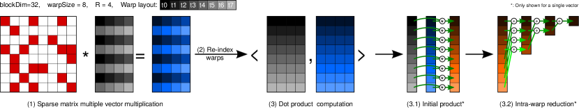
Figure 6: GPU implementation of SpMMV with on-the-fly dot product. Only a single thread block is shown.

The GPU kernels have been implemented using CUDA and hand-tuned for the Kepler architecture. There are well-known approaches for efficient SpMV (see, e.g.,  [12], [13] and references therein), but the augmented SpMMV kernel requires more effort. In particular for the implementation of on-the-fly dot product computations a sensible thread management is crucial. Figure 6 shows how the threads are mapped to the computation in the full aug_spmmv() kernel. For the sake of easier illustration, relevant architectural properties have been set to smaller values. In reality, the warpSize is 32 on Kepler and the maximum (and also the one which is used) blockDim is 1024. The threads in a warp are colored with increasing brightness in the figure. Note that this implementation is optimized towards relatively large vector blocks ($R\gtrsim 8$). In the following we explain the components of the augmented SpMMV kernel.

III-C1 SpMMV

The first step of the kernel is the SpMMV. In order to have coalesced access to the vector data, the warps must be arranged along block vector rows. Obviously, perfectly coalesced access can only be achieved for block vector widths which are at least as large as the warp size. We have observed, however, that smaller block widths achieve reasonable performance as well. In Fig. 6 the load of the vector data would be divided into two loads using half a warp each.

III-C2 Re-index warps

Operations involving reductions are usually problematic in GPU programming for two reasons: First, reductions across multiple blocks require thread synchronization among the blocks. Second, the reduction inside a block demanded the use of shared memory on previous NVIDIA architectures; this is no longer true for Kepler, however. This architecture implements shuffle instructions, which enable sharing values between threads in a warp without having to use shared memory [28]. For the dot product computation, the values which have to be shared between threads are located in the same vector (column of the block). This access pattern is different from the one used in step (1), where subsequent threads access different columns of the block. Hence, the thread indexing in the warps has to be adapted. Note that no data actually gets transposed but merely the indexing changes.

III-C3 Dot product

The actual dot product computation consists of two steps. Computing the initial product is trivial, as each thread only computes the product of the two input vectors. For the reduction phase, subsequent invocations of the shuffle instruction as implemented in the Kepler architecture are used. In total, $\mbox{log}_{2}(\texttt{warpSize})$ reductions are required for computing the full reduction result, which can then be obtained from the first thread. For the final reduction across vector blocks, CUB [29] has been used (not shown in Fig. 6).

IV Performance Models

In this section we apply the analysis from Section II-A to both our CPU and GPU implementation using an IVB CPU and a K20m GPU. We use a domain of size $100\times 100\times 40$ if not stated otherwise. This results in a matrix with $1.6\cdot 10^{6}$ rows. Thus, neither the matrix nor the vectors fit into any cache on either architecture.

IV-A CPU Performance Model

The relevant architectural bottleneck for SpM(M)V changes when increasing the block vector width. This assertion is confirmed by the intra-socket scaling performance (see Fig. 7) on IVB.

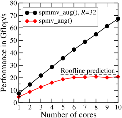
Figure 7: Socket scaling on IVB. The roofline prediction results from the measured attainable bandwidth $b$ from Table II, the code balance $B_{\mathrm{min}}$ from Eq. 6, and $\Omega=1$ (best case) in Eq. 9

The performance of the SpMV kernel is clearly bound by main memory bandwidth, saturating at a level (dashed line) which is reasonably close the roofline prediction obtained from Eq. 10. In contrast, the SpMMV kernel performance scales almost linearly within a socket. This indicates that the relevant bottleneck is either the bandwidth of some cache level or the in-core execution. It turns out that taking into account the L3 cache yields sufficient insight for a qualitative analysis of the performance bottlenecks (for recent work on refined roofline models for SpMMV see  [5] where both the L2 and L3 cache were considered). The roofline model (Eq. 9) can be modified by defining a more precise upper performance bound than $P^{\mathrm{peak}}$ for loops that are decoupled from memory bandwidth:

$$P^{*}=\mathrm{min}(P^{*}_{\mathrm{MEM}},P^{*}_{\mathrm{LLC}}).$$ (17)

Here, $P^{*}_{\mathrm{LLC}}$ is a performance limit for the last level cache, which is determined through benchmarking a down-sized problem where the whole working set (matrix and vectors) fits into the L3 cache of IVB while keeping the matrix as similar as possible to the memory-bound test case.

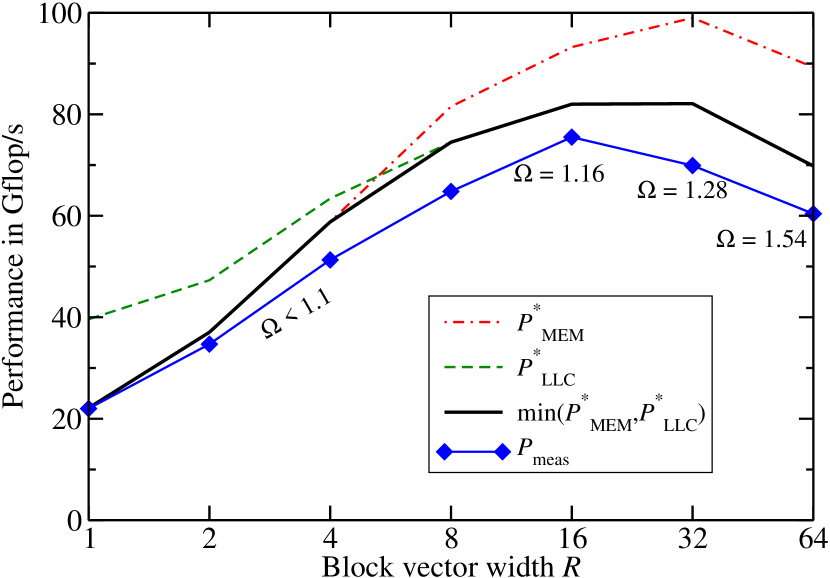
Figure 8: Custom roofline model for the augmented SpM(M)V kernel on IVB. Upper bounds for memory- and L3-boundedness, as well as the minimum of both, can be seen together with measured performance data.

A comparison of our custom roofline model with measured performance for the augmented SpM(M)V kernel is shown in Fig. 8. The shift of the relevant bottleneck can be identified: For small $R$ the kernel is memory-bound and the performance can be predicted by the standard roofline model (Eq. 9) with high accuracy. At larger $R$, the kernel’s execution decouples from main memory. A high quality performance prediction is more complicated in this region, but our refined model (Eq. 17) does not deviate by more than 15% from the measurement. A further observation from Fig. 8 is the impact of $\Omega$ (see annotations in the figure) on the code balance and on $P^{*}_{\mathrm{MEM}}$: For large $R$ the maximum achievable performance decreases although the minimum code balance (see Eq. 5) originally suggests otherwise.

IV-B GPU Performance Model

On the GPU, establishing a custom roofline model as in Eq. 17 is substantially more difficult because one can not use the GPU to full efficiency with a data set that fits in the L2 cache. Hence, the performance model for the GPU will be more of a qualitative nature. The Kepler architecture is equipped with two caches that are relevant for the execution of our kernel. Information on these caches can be found in  [28] and  [30]:

1. L2 cache: The L2 cache is shared between all SMX units. In the case of SpMV, it serves to alleviate the penalty of unstructured accesses to the input vector.

2. Read-only data cache: On Kepler GPUs there is a 48 KiB read-only data cache (also called texture cache) on each SMX. This cache has relaxed memory coalescing rules, which enables efficient broadcasting of data to all threads of a warp. It can be used in a transparent way if read-only data (such as the matrix and input vector in the aug_spmmv() kernel) is marked with both the const and __restrict__ qualifiers. In the SpMMV kernel, each matrix entry needs to be broadcast to the threads of a warp (see Section III-C for details), which makes this kernel a very good usage scenario for the read-only data cache.

In Section III-C we have described how the computation of dot products complicates the augmented SpMMV kernel. For our bottleneck analysis we thus consider the plain SpMMV kernel, the augmented SpMMV kernel (but without on-the-fly computation of dot products), and finally the full augmented SpMMV kernel. To quantify the impact of different memory system components we present the measured data volume when executing the simple SpMMV kernel (the qualitative observations are similar for the other kernels) for each of them in Fig. 9.

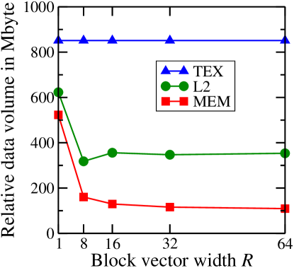
Figure 9: Measured data volume per block vector for different memory system components on the Kepler GPU running the simple SpMMV kernel.

The data traffic coming from the texture cache scales linearly with $R$ because the scalar matrix data is broadcast to the threads in a warp via this cache. The accumulated data volume across all hierarchy levels decreases for increasing $R$, which is due to the shrinking relative impact of the matrix on the data traffic. A potential further reason for this effect is higher load efficiency in the large $R$ range.

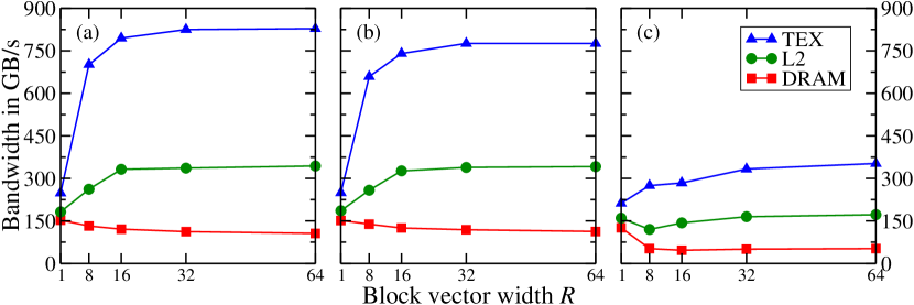
Figure 10: Measured bandwidth on the K20m GPU for different memory system components and kernels: (a) simple SpM(M)V kernel, (b) augmented SpM(M)V kernel without on-the-fly dot product computation, and (c) fully augmented SpM(M)V kernel.

Figure 10 shows DRAM, L2 cache, and Texture cache bandwidth measurements for the three kernels mentioned above. At $R=1$ the DRAM bandwidth is around 150 GB/s for the first two kernels, which is equal to the maximum attainable bandwidth on this device (see Table II; as expected, the kernel is memory bound. The bandwidths drawn from L2 and Texture cache are not much higher than the DRAM bandwidth in this case. With growing $R$ the DRAM bandwidth decreases while the bandwidths of L2 and Texture cache increase and eventually saturate. Thus, the relevant bottleneck is changed from DRAM to cache bandwidth as the computational intensity of the kernel goes up. For the fully augmented SpM(M)V kernel (right panel in Fig. 10), the qualitative curve shapes are similar to the other two kernels but all measured bandwidths are at a significantly lower level. This is caused by the dot product computation with all its issues (cf. Section III-C), making instruction latency the relevant bottleneck. However, this kernel still yields significantly higher performance than an implementation with separate dot product computation.

All these observations and conclusions coincide with the bottleneck analysis of the NVIDIA Visual Profiler. For all kernels it determines the DRAM bandwidth as the relevant bottleneck at $R=1$. At larger $R$ the L2 cache bandwidth is the bottleneck for the kernels without on-the-fly dot product calculations. Otherwise, i.e., when including dot products, the reported bottleneck is latency.

V Performance Results

V-A Symmetric Heterogeneous Execution

MPI is used as a communication layer for heterogeneous execution, and the parallelization across devices is done on a per-process basis. On a single heterogeneous node, simultaneous hybrid execution could also be implemented without MPI. However, using MPI already on the node level enables easy scaling to multiple heterogeneous nodes and portability to other heterogeneous systems. We use one process for each CPU/GPU in a node and OpenMP within CPU processes. A GPU process needs a certain amount of CPU resources for executing the host code and calling GPU kernels, for which one CPU core is usually sufficient. Hence, for the heterogeneous measurements in this paper one core per socket was “sacrificed” to its GPU. Each process runs in its own disjoint CPU set, i.e., there are no resource conflicts between the processes on a node.

The assembly of communication buffers in GPU processes is done in a GPU kernel. Only the elements which need to be transferred are copied to the host side before sending them to the communication partners. This is done via pinned memory in order to achieve a high transfer rate.

An intrinsic property of heterogeneous systems is that the components usually do not only differ in architecture but also in performance. For optimal load balancing this difference has to be taken into account for work distribution. In our execution environment a weight has to be provided for each process. From this weight we compute the amount of matrix/vector rows that get assigned to it.

V-B Node-Level Performance

Figure 11 shows the performance on a heterogeneous node for both architectures and all optimization stages. Single architectures solve for a $200\times 100\times 40$ domain, and a $400\times 100\times 40$ domain has been used for the heterogeneous runs.

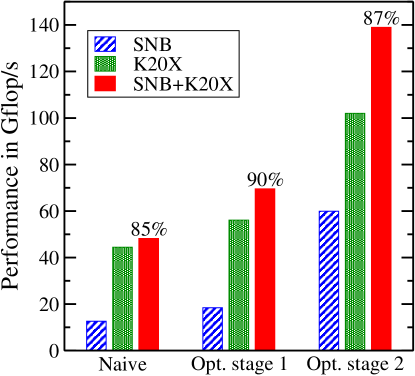
Figure 11: Node-level performance for each optimization stage on Piz Daint. The parallel efficiency of the heterogeneous execution is shown on top of the heterogeneous performance bars.

All weights have been tuned experimentally. However, a good guess is to calculate the weights from the single-device performance numbers. The maximum speed-up which can be achieved on a single node, i.e., the speed-up between the naive CPU-only implementation and the fully optimized heterogeneous version, is more than a factor of 10. However, a more realistic usage model of a GPU-equipped node is the naive GPU-only variant. Here, a speed-up of 2.3$\times$ can be achieved by algorithmic optimizations and careful implementation. On top of that, another 36% can be gained by enabling fully heterogeneous execution including the CPU. The parallel efficiency of the heterogeneous implementation with respect to the sum of the single-architecture performance levels tops out at 85–90%. The gap to optimal efficiency has two major reasons: First, the heterogeneous implementation includes communication over the relatively slow PCI Express bus. Second, one CPU core is used for GPU management. As the CPU kernel’s bottleneck is not memory bandwidth, excluding one core from the computation results in a performance decrease on the CPU side.

V-C Large-Scale Parallel Performance

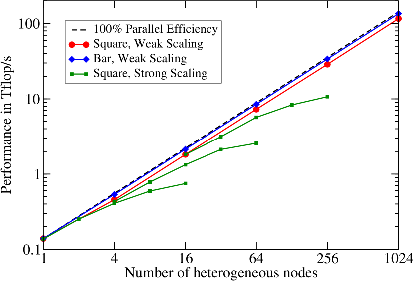
Figure 12: Weak scaling performance of the full KPM solver on Piz Daint for the “Square” and “Bar” test cases. The strong scaling curves show the performance for the “Square” case at a problem size as defined by the first point of each curve.

Figure 12 shows scaling data on up to 1024 nodes of Piz Daint for the topological material application scenario. For weak scaling we solve for two different domains: First, we consider a tile with fixed height $N_{z}=40$ and equally growing width and length (“Square”). The second test case represents a domain with fixed width $N_{y}=100$ and height $N_{z}=40$, and growing $N_{x}$ (“Bar”). For both cases, the baseline performance on a single node corresponds to the same system as in Fig. 11, i.e., a domain of size $400\times 100\times 40$. In the “Square” test, the $y$ dimension increases to 400 when going to four nodes in order to have a quadratic tile. The drop in parallel efficiency in this region is a result of the growing number of processors in the $y$ direction, which leads to an increase in communication volume. On larger node counts the number of nodes quadruples in each step while the extent in $x$ and $y$ direction doubles. In the “Bar” test, the $x$ dimension increases by 400 for each added node. The strong scaling curves always represent the performance for a fixed problem size as given by the data set at the first point of each curve. The largest system solved in these runs is described by a matrix with over $6.5\cdot 10^{9}$ rows.

Looking at the non-blocked version of the algorithm (Fig. 4), one may argue that there is no dependency between outer loop iterations, and highly efficient parallelization should be easily achieved by just running $R$ instances of the loop code. However, our optimization stage 2 has shown that it is just the incorporation of the $R$ loop that enables the algorithm to decouple from the memory bandwidth; solving the problem in “throughput mode” will thus incur a significantly higher overall cost. We illustrate this difference in Table III, which summarizes the resource requirements of three different variants to solve the largest problem: the augmented SpMV from Fig. 4, the augmented SpMMV with a global reduction over dot products in each iteration (cf. Section I), and the final optimized version with a single global reduction at the end.

Version	Tflop/s	Nodes	Node hours
aug_spmv()	14.9	288	164
aug_spmmv()∗	107	1024	81
aug_spmmv()	116	1024	75

TABLE III: Overview of required resources for solving the largest system with $R=32$ and $M=2000$. The non-blocked version aug_spmv() has been run in throughput mode. aug_spmmv()^∗ indicates a version where a global reduction over the dot products has been done in each iteration instead of once at the very end.

The data shows impressively that the embarrassingly $R$-parallel version is more than a factor of two more expensive in terms of compute resources (node hours) than the optimal version. Reducing the number of global reductions increases the performance by 8%. Note that this factor strongly depends on the communication patterns and can be substantially higher for other matrices.

VI Conclusion and Outlook

In this work we have performed systematic, model-guided performance engineering for the KPM-DOS algorithm leading to a substantial increase in node-level performance on the CPU and the GPU. This was achieved by crafting a problem-specific loop kernel that has all required operations fused in and achieves minimal theoretical code balance. The performance analysis of the optimized algorithm on the CPU and on the GPU revealed that the optimizations led to a complete decoupling from the main memory bandwidth for relevant application cases on both the CPU and the GPU. Finally we have embedded our optimized node-level kernel into a massively parallel, heterogeneous application code. For the interesting application scenario of topological insulators we have demonstrated the scalability, performance, and resource efficiency of the implementation on up to 1024 nodes of a petascale-class Cray XC30 system. All software which has been developed within the scope of this work is available for download [10].

In the future we will apply our findings and code to other blocked sparse linear algebra algorithms besides KPM. Several open questions remain regarding possible improvements of our approach. A future step could be to determine the process weights for heterogeneous execution automatically and take this burden away from the user. Furthermore, heterogeneous MPI communication is a field which has room for improvement. A promising optimization is to establish a pipeline for this GPU-CPU-MPI communication, i.e., download parts of the communication buffer to the host and transfer previous chunks via the network at the same time. It will also be worthwhile investigating further optimization techniques such as cache blocking [31] for the CPU implementation of SpMMV. Although the Intel Xeon Phi coprocessor is already supported in our software, we still have to carry out detailed model-driven performance engineering for this architecture and the KPM application.

References

- [1] (2014, November) TOP500 Supercomputer Sites. [Online]. Available: http://www.top500.org
- [2] MAGMA: Matrix algebra on GPU and multicore architectures. [Online]. Available: http://icl.cs.utk.edu/magma/
- [3] W. D. Gropp, D. K. Kaushik, D. E. Keyes, and B. F. Smith, “Towards realistic performance bounds for implicit CFD codes,” in Proceedings of Parallel CFD’99. Elsevier, 1999, pp. 233–240.
- [4] X. Liu, E. Chow, K. Vaidyanathan, and M. Smelyanskiy, “Improving the performance of dynamical simulations via multiple right-hand sides,” in Proceedings of the 2012 IEEE International Parallel and Distributed Processing Symposium, May 2012. IEEE Computer Society, 2012, pp. 36–47.
- [5] H. M. Aktulga, A. Buluç, S. Williams, and C. Yang, “Optimizing sparse matrix-multiple vectors multiplication for nuclear configuration interaction calculations,” in Proceedings of the 2014 IEEE International Parallel and Distributed Processing Symposium, May 2012. IEEE Computer Society, 2014.
- [6] R. N. Silver, H. Röder, A. F. Voter, and D. J. Kress, “Kernel polynomial approximations for densities of states and spectral functions,” J. Comp. Phys., vol. 124, p. 115, 1996.
- [7] A. Weiße, G. Wellein, A. Alvermann, and H. Fehske, “The kernel polynomial method,” Rev. Mod. Phys., vol. 78, pp. 275–306, Mar 2006. [Online]. Available: http://dx.doi.org/10.1103/RevModPhys.78.275
- [8] E. di Napoli, E. Polizzi, and Y. Saad, “Efficient estimation of eigenvalue counts in an interval,” 2013, preprint. [Online]. Available: http://arxiv.org/abs/1308.4275
- [9] O. Bhardwaj, Y. Ineichen, C. Bekas, and A. Curioni, “Highly scalable linear time estimation of spectrograms - a tool for very large scale data analysis,” 2013, poster at 2013 ACM/IEEE International Conference on High Performance Computing Networking, Storage and Analysis.
- [10] GHOST: General, Hybrid, and Optimized Sparse Toolkit. [Online]. Available: http://tiny.cc/ghost
- [11] R. Barrett, M. Berry, T. F. Chan, J. Demmel, J. Donato, J. Dongarra, V. Eijkhout, R. Pozo, C. Romine, and H. V. der Vorst, Templates for the Solution of Linear Systems: Building Blocks for Iterative Methods. Philadelphia, PA: SIAM, 1994.
- [12] N. Bell and M. Garland, “Implementing sparse matrix-vector multiplication on throughput-oriented processors,” in Proceedings of the Conference on High Performance Computing Networking, Storage and Analysis, ser. SC ’09. New York, NY, USA: ACM, 2009, pp. 18:1–18:11. [Online]. Available: http://doi.acm.org/10.1145/1654059.1654078
- [13] M. Kreutzer, G. Hager, G. Wellein, H. Fehske, and A. R. Bishop, “A unified sparse matrix data format for efficient general sparse matrix-vector multiplication on modern processors with wide SIMD units,” SIAM J. Sci. Comput., vol. 36, no. 5, pp. C401–C423, 2014. [Online]. Available: http://epubs.siam.org/doi/abs/10.1137/130930352
- [14] R. W. Vuduc, “Automatic performance tuning of sparse matrix kernels,” Ph.D. dissertation, University of California, Berkeley, 2003.
- [15] H. Anzt, S. Tomov, and J. Dongarra, “Accelerating the LOBPCG method on GPUs using a blocked sparse matrix vector product,” University of Tennessee Innovative Computing Laboratory Technical Report UT-CS-14-731, October 2014. [Online]. Available: http://www.eecs.utk.edu/resources/library/589
- [16] CUDA sparse matrix library (cuSPARSE). NVIDIA. [Online]. Available: https://developer.nvidia.com/cuSPARSE
- [17] K. K. Matam, S. R. K. B. Indarapu, and K. Kothapalli, “Sparse matrix-matrix multiplication on modern architectures,” in 19th International Conference on High Performance Computing, HiPC 2012, Pune, India, December 18-22, 2012, 2012, pp. 1–10. [Online]. Available: http://dx.doi.org/10.1109/HiPC.2012.6507483
- [18] S. Zhang, S. Yamagiwa, M. Okumura, and S. Yunoki, “Kernel polynomial method on GPU,” International Journal of Parallel Programming, vol. 41, no. 1, pp. 59–88, 2013. [Online]. Available: http://dx.doi.org/10.1007/s10766-012-0204-y
- [19] M. Z. Hasan and C. L. Kane, “Topological insulators,” Rev. Mod. Phys., vol. 82, pp. 3045–3067, Nov 2010. [Online]. Available: http://link.aps.org/doi/10.1103/RevModPhys.82.3045
- [20] G. Schubert, H. Fehske, L. Fritz, and M. Vojta, “Fate of topological-insulator surface states under strong disorder,” Phys. Rev. B, vol. 85, p. 201105, May 2012.
- [21] A. Pieper, R. L. Heinisch, G. Wellein, and H. Fehske, “Dot-bound and dispersive states in graphene quantum dot superlattices,” Phys. Rev. B, vol. 89, p. 165121, Apr 2014.
- [22] M. Galgon, L. Krämer, B. Lang, A. Alvermann, H. Fehske, and A. Pieper, “Improving robustness of the FEAST algorithm and solving eigenvalue problems from graphene nanoribbons,” Proc. Appl. Math. Mech., vol. 14, no. 1, pp. 821–822, 2014. [Online]. Available: http://dx.doi.org/10.1002/pamm.201410391
- [23] J. Treibig, G. Hager, and G. Wellein, “LIKWID: A lightweight performance-oriented tool suite for x86 multicore environments,” in Proceedings of the 2010 39th International Conference on Parallel Processing Workshops, ser. ICPPW ’10. Washington, DC, USA: IEEE Computer Society, 2010, pp. 207–216. [Online]. Available: http://dx.doi.org/10.1109/ICPPW.2010.38
- [24] NVIDIA Profiler. NVIDIA. [Online]. Available: http://docs.nvidia.com/cuda/profiler-users-guide
- [25] S. Williams, A. Waterman, and D. Patterson, “Roofline: An insightful visual performance model for multicore architectures,” Commun. ACM, vol. 52, no. 4, pp. 65–76, Apr. 2009. [Online]. Available: http://doi.acm.org/10.1145/1498765.1498785
- [26] M. Röhrig-Zöllner, J. Thies, M. Kreutzer, A. Alvermann, A. Pieper, A. Basermann, G. Hager, G. Wellein, and H. Fehske, “Increasing the performance of the Jacobi-Davidson method by blocking,” 2014, submitted to SIAM J. Sci. Comput. [Online]. Available: http://elib.dlr.de/89980/
- [27] V. Volkov and J. W. Demmel, “Benchmarking GPUs to tune dense linear algebra,” in Proceedings of the 2008 ACM/IEEE Conference on Supercomputing, ser. SC ’08. Piscataway, NJ, USA: IEEE Press, 2008, pp. 31:1–31:11. [Online]. Available: http://dl.acm.org/citation.cfm?id=1413370.1413402
- [28] Kepler GK110 Architecture Whitepaper. NVIDIA. [Online]. Available: http://www.nvidia.com/content/PDF/kepler/NVIDIA-Kepler-GK110-Architecture-Whitepaper.pdf
- [29] CUB. NVIDIA Research. [Online]. Available: http://nvlabs.github.io/cub/
- [30] Kepler Tuning Guide. NVIDIA. [Online]. Available: http://docs.nvidia.com/cuda/kepler-tuning-guide
- [31] E.-J. Im, K. Yelick, and R. Vuduc, “Sparsity: Optimization framework for sparse matrix kernels,” Int. J. High Perform. Comput. Appl., vol. 18, no. 1, pp. 135–158, Feb. 2004. [Online]. Available: http://dx.doi.org/10.1177/1094342004041296