Energy-Spectral Efficiency Trade-off for a Massive SU-MIMO System with Transceiver Power Consumption
Abstract
We consider a single user (SU) massive MIMO system with multiple antennas at the transmitter (base station) and a single antenna at the user terminal (UT). Taking transceiver power consumption into consideration, for a given spectral efficiency (SE) we maximize the energy efficiency (EE) as a function of the number of base station (BS) antennas , resulting in a closed-form expression for the optimal SE-EE trade-off. It is observed that in contrast to the classical SE-EE trade-off (which considers only the radiated power), with transceiver power consumption taken into account, the EE increases with increasing SE when SE is sufficiently small. Further, for a fixed SE we analyze the impact of varying cell size (i.e., equivalently average channel gain ) on the optimal EE. We show the interesting result that for sufficiently small , the optimal EE decreases as with decreasing . Our analysis also reveals that for sufficiently small SE (or large ), the EE is insensitive to the power amplifier efficiency.
I Introduction
There has been a recent surge of interest on energy efficient “green communication” systems, arising out of environmental/cost concerns due to the ever increasing power consumption of cellular systems [1]. The total system capacity and energy efficiency is expected to improve significantly in going from the current 4G systems to the next generation cellular communication systems (5G) [2]. Massive MIMO systems has recently been proposed as a possible 5G technology [3]. Massive MIMO refers to a communication system where a base station (BS) with antennas (several tens to hundred) communicates coherently with user terminals (few tens) on the same time-frequency resource [4].
In [5, 6] the spectral efficiency (SE) versus energy efficiency (EE) trade-off of massive MIMO system has been studied. However, in these works only the power consumed by the power amplifiers (PA) has been considered. With large the total power consumed by the RF transceivers at the BS will becomes significant and must therefore be taken into consideration [7]. The impact of transceiver power consumption on the EE has been studied in several recent papers. However, none of them have derived any closed-form expression for the SE-EE trade-off curve with transceiver power consumption, not even for the single user case with perfect channel state information (CSI). Also none of these recent works have analytically studied the variation in the EE with cell size (for a fixed SE). In the following we briefly discuss the contribution of these recent works.
In [8] it is shown that the EE of uplink MIMO systems can be optimized by selectively turning off antennas at the user terminal (UT). In[9], the authors optimize the EE of downlink massive MIMO systems with respect to (w.r.t.) the number of BS antennas. It is shown that the EE is a quasi-concave function of the number of BS antennas. In [10] downlink massive MIMO systems are considered, and for a fixed the EE is maximized w.r.t. the total power radiated from the BS and the number of UTs (). However, results in [8, 9, 10] are based on numerical simulations and therefore they provide little insight on the exact SE-EE trade-off. In [11, 12] the authors consider the downlink of multi-user MIMO systems, and for the ZF precoder they analytically optimize the EE separately w.r.t. , and the total radiated power. They show the very interesting result that massive MIMO must be used to increase EE only when interference suppressing multi-user precoding schemes (e.g., ZF, MMSE) are used. However, the analytical results in [11] and [12] cannot be used to derive the exact optimal SE-EE trade-off, since they do not explicitly find the optimal EE for any given SE. In [13], for the uplink multi-user MIMO system with a ZF multi-user detector at the BS, the author studies the impact of varying power consumption parameters (PCPs) on the optimal EE (i.e., EE optimized w.r.t. for a given/fixed SE). It is shown that for sufficiently large values of the PCPs it is optimal to have few BS antennas communicating with a single UT, and vice-versa. However since the power consumption model in [13] does not consider SE-dependent power consumption due to channel coding/decoding and backhaul, the results in [13] cannot be used to derive the optimal SE-EE trade-off.
In this paper, we consider the downlink of a single user (SU) system with antennas at the BS. The UT has a single antenna and the BS is assumed to have perfect CSI. For this set-up, none of the previous works have derived an analytical expression for the optimal SE-EE trade-off. Similarly no analytical study on the variation in the optimal EE with the cell size (equivalently average channel gain) exists. The main contribution of our paper is the derivation of a closed-form expression for the optimal SE-EE trade-off (for a fixed average channel gain). We observe that for a sufficiently small SE, the EE increases linearly with SE. This result is in contrast with the classical result where only PA power consumption is taken into consideration, for which the EE always decreases monotonically with increasing SE [6].
For a fixed SE, we also analyze the exact variation in the optimal EE with changing average channel gain (). It is observed that for sufficiently small , with decreasing the EE decreases proportionally to . Through analysis we derive a closed-form expression for the fraction of the total system power consumed by the PAs, as a function of SE (for a fixed ), and also as a function of (for a fixed SE). It is observed that for sufficiently large SE (or small ) this fraction is close to half, whereas for sufficiently small SE (or large ) this fraction is close to zero. Therefore, for sufficiently small SE (or large ) the EE is insensitive to the PA efficiency. Hence low efficiency PAs (which are generally highly linear [14]) can be used. To the best of our knowledge this study on the variation in the fraction of total power consumed by the PAs as a function of SE (or ) has not been reported so far in previous works.
Notations: and denote the set of Complex and Real numbers respectively. denotes the expectation operator. denotes the complex conjugate transpose operation. denotes the set of all positive integers. denotes the circular symmetric complex Gaussian distribution. Also, denotes the Euclidean norm of .
II System Model
Let us consider a single user downlink MISO system, where a multiple antenna base station (BS) communicates with a single antenna user terminal (UT). The received signal at the UT is thus given by
| (1) |
where is the complex baseband channel gain vector, with being the channel gain from the BS antenna to the UT. We assume a Rayleigh flat fading channel, i.e., , .
Here, is the total transmitted power and is the transmitted signal vector ( is transmitted from the BS antenna). Let be the information symbol to be communicated to the UT (). With conjugate beamforming [6], we have111Perfect CSI at the BS is assumed.
| (2) |
In (1), models the geometric attenuation and lognormal shadow fading and represents the additive complex circular symmetric Gaussian white noise at the UT (i.e., ). Here is the noise power spectral density and is the channel bandwidth. The above model can also be applied to wide-band channels, where OFDM is used.
The power consumption sources in this model can be categorized as follows: (a) RF power consumption ( in Watt) in the RF chains, power amplifiers (PAs) and oscillator circuits, (b) power consumption ( in Watt) due to conjugate beamforming, (c) fixed power consumption ( in Watt) in the baseband processors, and (d) load/data-rate dependent power consumption ( in Watt/bits/s), e.g. channel coding, decoding and backhaul processing. Total load-dependent power consumption is thus computed to be , where is the spectral efficiency (SE) of the system, measured in bits/s/Hz. So, the total system power consumption is given by
| (3) |
The RF power consumption can be further subdivided into: (i) per antenna RF chain power consumption at the BS () and UT (), (ii) power consumption by the local oscillators (), and (iii) PA power consumption ( models the power efficiency222Power efficiency of PA is the fraction of input power (consumed power), that is radiated by the antenna [10]. Further we also assume that the PAs operate in the linear region of their transfer characteristics [13].). Therefore,
| (4) |
From (2), it is clear that the conjugate beamformer requires a total of operations per channel use for scaling and multiplication [15]. Assuming Joule is consumed for each operation, the total energy consumed for operations is Joule. Since operations are performed in seconds, the overall power consumption for beamforming is Watt. Substituting the expressions for (from (4)) and in (3), we get
| (5) | |||||
where .
The energy efficiency (EE) in bits/Joule is defined as
| (6) |
Multiplying both sides of (6) by , we get , where is the normalized EE, defined as . Using (5) we have
| (7) |
Clearly, is a function of , and the system parameter vector333This normalization of the PCPs () with is motivated from the fact that power consumption in bandlimited transceiver circuits is typically proportional to [16]. , where
| (8) |
where is the transmitted SNR444 is a function of and , but we do not write it explicitly for sake of brevity..
III Energy and Spectral Efficiency Trade-off
Since we are interested in understanding the EE-SE trade-off, in this section, we study the optimization of with respect to the number of BS antennas, , for a fixed and . The ergodic capacity of the system in (1) is given by
| (10) |
Clearly, for a given , increases monotonically with increasing . Therefore, a unique function exists such that for any , satisfies the equality . With , the inverse energy efficiency (from (9)) is therefore given by
| (11) |
For a given , the exact optimal EE of the system (when the system is capacity achieving, i.e., ) is given by
| (12) |
Lemma 1: It can be shown from (10) that
| (13) |
Proof:
See Appendix A. ∎
Remark 1: It is clear that is an achievable information rate, lower than the ergodic capacity. With , for a given and , the required transmit SNR is given by
| (14) |
The corresponding system energy efficiency with as the information rate would be
| (15) |
where . ∎
The optimization in (III) is difficult to solve analytically, due to non-availability of closed form expression for . However, we know that since for a given , , it follows that . In the following we discuss the tightness of this lower bound on . It follows from Lemma 1 that
| (16) |
Since, for (i.e., for massive MIMO systems), from (16) it follows that for . Using this fact and comparing the R.H.S. in (11) and (15) we see that for , . The tightness of this approximation has been exhaustively validated through numerical simulations (e.g. see Fig. 1). We therefore propose to analyze the optimal EE with . This optimization is given by
| (17) |
The optimization problem in (III) is still difficult to solve in closed form, because . However, a near optimal closed-form solution to the optimization problem in (III) can be obtained through analysis, if the constraint on is relaxed so that . For and ,
| (18) |
Therefore for , is convex, with a unique global minimum occurring at
| (19) |
With , the proposed near-optimal energy efficiency is then given by
| (20) | |||||
IV Study of the EE-SE Trade-off
In this section we study the EE-SE trade-off in (20) and characterize its behaviour for small and large values of SE. Throughout this study of the trade-off, we assume and to be fixed.
Proposition 1: For a sufficiently small , i.e.,
| (21) |
we have
| (22) |
i.e., increases linearly with increasing . Also for any satisfying (21), we have
| (23) |
Proof:
Remark 2: In the following we explain the result of proposition 1. When is sufficiently small, the required power to be radiated from the PAs is also small. Therefore the total system power consumption is dominated by the power consumed by the RF chains at the BS and UT and the fixed power consumption (e.g. oscillators and baseband processors etc.). With increase in , the power consumed by the RF chains at the BS will increase and therefore EE will decrease. This shows that for sufficiently small , it is optimal to have only a single BS antenna (i.e., non-massive MIMO regime, see (23)).
From the above discussion we know that with a sufficiently small , it is expected that the PA power consumption is a small fraction of the total system power consumption. Since the number of BS antennas is fixed to one, the total system power consumption will be almost constant with increasing (as long as is sufficiently small). This implies that the overall EE will increase with increasing (see Fig. 2). This result is in contrast with the classical result where the EE always decreases with increasing SE when only PA power consumption is considered. ∎
Proposition 2: For a sufficiently large , i.e.,
| (24) |
decreases monotonically with increasing and that .
Further increases exponentially with increasing .
Proof:
For any satisfying (24), the denominator of the R.H.S. of (20) is dominated by . Therefore under the condition in (24), we get
| (25) |
Remark 3: As , the power consumed by the PAs, increase at a rate proportional to for a fixed (see (14)). Increasing will increase the array gain, which in turn will reduce the PA power consumption. If (), then increases at a rate faster than and the total power consumption is dominated by the RF chain power consumption at the BS (see (15)), which increases linearly with . Similarly if , i.e., increases at a rate slower than , the total system power consumption is dominated by the power consumed by the PA, which increases as . In either case, the total power consumption increases as . Therefore, it is optimal to have , i.e., (massive MIMO regime). ∎
| (26) |
V Impact of Cell Size on EE (Fixed SE and PCPs)
In this section we analyze the impact of (i.e., average channel gain) on the EE of the system for a fixed and fixed power consumption parameters . We assume that the UT is at the cell edge and therefore a large value of corresponds to a small cell size and vice versa. Since depends on , using (20) the unnormalized near optimal EE is given by (26). Similarly from (19) the near optimal is given by
| (27) |
Proposition 3: If is sufficiently large, i.e.,
| (28) |
then the near optimal EE, becomes insensitive to changes in . Further, for any satisfying (28), we have .
Proof:
From (26) it is evident that for any satisfying (28), the total power consumption would be dominated by . Using (28) in (26), we therefore have
| (29) |
Remark 4: For small cell size, the effective channel gain could be large, resulting in reduction in the required transmit power. Thus the power consumed by the PAs will decrease with increasing and the total system power consumption will eventually be dominated by the other sources of power consumption (including the power consumed by the RF antennas at the BS).
With increase in , the power consumed by the RF chains at the BS will increase and dominate the total system power consumption. Hence with increasing the EE will decrease. This shows that for sufficiently large (i.e. for small cell size) it is optimal to have only a single antenna at the BS.
With a single antenna at the BS, the total system power consumption is almost constant with increasing . This is so because with increasing the power consumption by PAs is increasingly dominated by the other sources of power consumption (which are independent of ). Hence for a fixed SE, the EE is insensitive to changes in the cell size as long as the cell size is sufficiently small (see also the non-massive MIMO regime in Fig. 1). ∎
Proposition 4: If is sufficiently small, i.e.,
| (30) | |||||
then with decreasing . Furthermore, , i.e., increases with decreasing .
Proof:
It is clear that for small satisfying (30), the denominator of (26) is dominated by the L.H.S. of (30). Using this fact in (26), we get
| (31) |
i.e., . Further from (27), it is evident that as . ∎
Remark 5: For fixed and , the required radiated power from the BS increases linearly with decreasing . Therefore for sufficiently small , the PA power consumption will dominate the total power consumption. Hence with a fixed , the energy efficiency would decrease linearly with decreasing . By increasing , we can reduce the PA power consumption due to increase in array gain. However, increasing will also increase the RF power consumption. It follows that the best trade-off is observed by increasing with decreasing (i.e., massive MIMO regime). With , both the PA and the RF power consumptions will increase at the same rate (i.e. ) with decreasing . Therefore, as (sufficiently small) decreases, the overall EE will decrease as555This same conclusion has also been drawn in [13] through heuristic arguments but no analytical proof has been presented. . Note that by varying with decreasing , the EE reduces at a slower rate (i.e., ) compared to a linear decrease for the scenario where is fixed (see also Fig. 1). ∎
VI Effect of SE and on the PA Design
In this section we analyze the impact of SE and on the required power efficiency of the PAs at the BS. We observe that for sufficiently large SE or large cell size the PAs must be highly efficient. In contrast to this, for sufficiently small SE or small cell size the EE is insensitive to the PA efficiency and therefore low efficiency PAs can be used. We firstly compute the fraction of the total system power consumption that is consumed by the PAs. The total system power consumption with near optimal is given by the denominator of the R.H.S. in (26), i.e.
| (32) | |||||
Similarly, with near optimal , the power consumption by the PAs is given by
where follows from (9), follows from (14), and follows from (27). The fraction of the total power consumed by the PAs, is therefore given by
| (33) |
Remark 6: For sufficiently small (i.e. large cell size) or for sufficiently large , from (33) it is clear that (with or , see also Fig. 3). This result is expected since for large cell size or large , the total power consumption is equally dominated by the RF power consumption at the BS (including beamformer) and the PA power consumption. Therefore in the massive MIMO regime highly efficient PAs must be used. ∎
Remark 7: From (33) it is clear that with or (i.e. small SE or small cell size) we have . From Remark 2 and Remark 4 we know that for small SE or small cell size it is EE optimal to operate in the non-massive MIMO regime, i.e., . With , the power consumption by the RF chain is constant. However as or , the PA power consumption goes to zero. Hence the fraction of total power consumed by the PAs is negligible as or . This leads us to the conclusion that the EE is insensitive to the PA power efficiency as or (see also Fig. 3). Hence in the non-massive MIMO regime low efficiency PAs can be used. ∎
VII Numerical Results
In this section, we numerically compute the exact optimal EE and the exact optimal . We present simulation curves in support of the analysis done in sections III to VI. Throughout this section, we assume W/Hz, W, W/Gbits/s, W, W, MHz, PA power efficiency = , and J. These are based on realistic values obtained from prior works [17, 18, 19, 20].
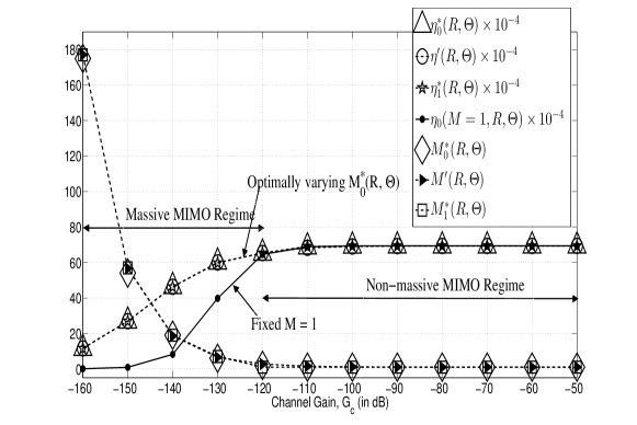
In Fig. 1 we study the impact of on the EE of the system for a fixed SE ( bps/Hz). We observe that it is EE optimal to have a single antenna at the BS when is sufficiently large ( dB). In this non-massive MIMO regime, the EE is observed to be almost constant with varying . These observations support the analytical findings of Proposition 3 (see also Remark 4).
With decreasing ( is sufficiently small), it is observed that the EE decreases and the optimal number of BS antennas increases (i.e. massive MIMO regime). We have also plotted the EE, , achieved when the number of BS antenna is fixed to one (i.e., does not vary with ). It is observed that decreases at a much faster rate compared to the optimal EE (see Remark 5). For instance at dB we have and at dB we have . Further, in Fig. 1 it can be seen that the proposed near optimal EE in (26) is close to the exact optimal EE, i.e., . This justifies the discussion in section III on the near optimal relaxation of the exact EE optimization in (III) by the optimization in (19).
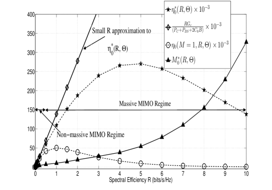
In Fig. 2, we plot the exact optimal EE-SE trade-off for a fixed dB. It is observed that the EE increases linearly with for sufficiently small (compare the curve with black stars to that with diamonds). This observation supports Proposition 1 and Remark 2. With increasing , the EE decreases eventually as is suggested in Proposition 2 and Remark 3.
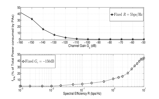
In Fig. 3 we plot the fraction of the total system power consumed by PAs () as a function of : (i) varying , with fixed bits/s/Hz and (ii) varying with fixed dB. For sufficiently small or large , it is observed that is small and therefore low efficiency PAs can be used. In contrast for the massive MIMO regime (i.e. sufficiently large or small ), we observe that almost of the total system power consumption is due to the PAs and therefore power efficient PAs must be used. These observations support the analytical findings in Remarks 6 and 7.
Appendix A Proof of Lemma 1
Since is distributed with degrees of freedom, we have
| (34) |
Since is concave in , from Jensen’s inequality it follows that
| (35) | |||||
where the last step follows from (34). Similarly, is convex in , and therefore from Jensen’s inequality we have
| (36) | |||||
References
- [1] S. Tombaz, A. Vastberg, and J. Zander, “Energy- and Cost-efficient Ultra-high-capacity Wireless Access,” IEEE Trans. Wireless Commun., vol. 18, no. 5, pp. 18–24, October 2011.
- [2] J. Andrews, S. Buzzi, W. Choi, S. Hanly, A. Lozano, A. Soong, and J. Zhang, “What Will 5G Be?” IEEE J. Sel. Areas Commun., vol. 32, no. 6, pp. 1065–1082, June 2014.
- [3] F. Rusek, D. Persson, B. K. Lau, E. Larsson, T. Marzetta, O. Edfors, and F. Tufvesson, “Scaling Up MIMO: Opportunities and Challenges with Very Large Arrays,” IEEE Signal Process. Mag., vol. 30, no. 1, pp. 40–60, Jan 2013.
- [4] T. Marzetta, “Noncooperative Cellular Wireless with Unlimited Numbers of Base Station Antennas,” IEEE Trans. Wireless Commun., vol. 9, no. 11, pp. 3590–3600, November 2010.
- [5] H. Q. Ngo, E. Larsson, and T. Marzetta, “Energy and Spectral Efficiency of Very Large Multiuser MIMO Systems,” IEEE Trans. Commun., vol. 61, no. 4, pp. 1436–1449, April 2013.
- [6] H. Yang and T. Marzetta, “Performance of Conjugate and Zero-Forcing Beamforming in Large-Scale Antenna Systems,” IEEE J. Sel. Areas Commun., vol. 31, no. 2, pp. 172–179, February 2013.
- [7] E. Björnson, J. Hoydis, M. Kountouris, and M. Debbah, “Massive MIMO systems with Non-ideal Hardware: Energy Efficiency, Estimation and Capacity Limits,” 2014, Submitted to IEEE Trans. Info. Theory. [Online]. Available. http://arxiv.org/abs/1307.2584v3.
- [8] G. Miao, “Energy-Efficient Uplink Multi-User MIMO,” IEEE Trans. Wireless Commun., vol. 12, no. 5, pp. 2302–2313, May 2013.
- [9] D. Ha, K. Lee, and J. Kang, “Energy Efficiency Analysis with Circuit Power Consumption in massive MIMO Systems,” in Personal Indoor and Mobile Radio Communications (PIMRC), 2013 IEEE 24th International Symposium on, Sept 2013, pp. 938–942.
- [10] H. Yang and T. Marzetta, “Total energy efficiency of cellular large scale antenna system multiple access mobile networks,” in Online Conference on Green Communications (GreenCom), 2013 IEEE, Oct 2013, pp. 27–32.
- [11] E. Björnson, L. Sanguinetti, J. Hoydis, and M. Debbah, “Designing Multi-User MIMO for Energy Efficiency: When is Massive MIMO the Answer?” in Proc. IEEE Wireless Communications and Networking Conference (WCNC), April 2014.
- [12] E. Björnson, L. Sanguinetti, J. Hoydis, and M. Debbah, “Optimal Design of Energy-Efficient Multi-User MIMO Systems: Is Massive MIMO the Answer?” 2014, Submitted to IEEE Trans. Wireless Commun. [Online]. Available. http://arxiv.org/abs/1403.6150v1.
- [13] S. K. Mohammed, “Impact of Transceiver Power Consumption on the Energy Efficiency Spectral Efficiency Tradeoff of Zero-Forcing Detector in Massive MIMO Systems,” 2014, Submitted to IEEE Trans. Commun. [Online]. Available. http://arxiv.org/abs/1401.4907v2.
- [14] S. C. Cripps, RF Power Amplifiers for Wireless Communications. Artech Publishing House, 1999.
- [15] L. Vandenberghe, “Applied Numerical Computing.” [Online]: www.seas.ucla.edu/ vandenbe/103/lectures/lu.pdf.
- [16] A. Mezghani and J. Nossek, “Modeling and minimization of transceiver power consumption in wireless networks,” in Smart Antennas (WSA), 2011 International ITG Workshop on, Feb 2011, pp. 1–8.
- [17] G. Auer, O. Blume, V. Giannini, I. Godor, M. Imran, Y. Jading, E. Katranaras, M. Olsson, D. Sabella, P. Skillermark, and W. Wajda, D2.3: Energy Efficiency Analysis of the Reference Systems, Areas of Improvements and Target Breakdown. INFSO-ICT-247733 EARTH, 2012, [Online]. Available: http://www.ict-earth.eu/.
- [18] A. Mezghani and J. Nossek, “Power Efficiency in Communication Systems from a Circuit Perspective,” in Circuits and Systems (ISCAS), 2011 IEEE International Symposium on, May 2011, pp. 1896–1899.
- [19] R. V. R. Kumar and J. Gurugubelli, “How green the LTE technology can be?” in Wireless Communication, Vehicular Technology, Information Theory and Aerospace Electronic Systems Technology (Wireless VITAE), 2011 2nd International Conference on, Feb 2011, pp. 1–5.
- [20] The Green List, November 2013, http://www.green500.org/lists/green2013/.