Semileptonic $B\rightarrow\bar{D}$ transition in nuclear medium


K. Azizi1   , N. Er2, H. Sundu3
1 Department of Physics, Doğuş University, Acıbadem-Kadıkây, 34722 İstanbul, Turkey
2 Department of Physics, Abant Δ°zzet Baysal University, GΓΆlkΓΆy KampΓΌsΓΌ, 14980 Bolu, Turkey
3 Department of Physics, Kocaeli University, 41380 Δ°zmit, Turkey
e-mail: kazizi@dogus.edu.tre-mail: nuray@ibu.edu.tre-mail: hayriye.sundu@kocaeli.edu.tr

We study the semileptonic tree-level $B\rightarrow\bar{D}$ transition in the framework of QCD sum rules in nuclear medium. In particular, we calculate the in-medium form factors entering the transition matrix elements defining this decay channel. It is found that the interactions of the participating particles with the medium lead to a considerable suppression in the branching ratio compared to the vacuum.

PACS number(s):13.20.He, 21.65.Jk, 11.55.Hx

1 Introduction

It is well-known that the semileptonic $B$ meson decay channels are excellent frameworks to calculate the standard model parameters, confirm its validity, understand the origin of CP violation and search for new physics effects. There are many theoretical and experimental studies devoted to the semileptonic tree-level $B\rightarrow D$ transition in vacuum for many years. After the BABAR [1] measurement of the ratio of branching fractions in $\tau$ and $\ell=\mu,e$ channels, i.e. ${\cal R}(D)={\cal B}(\overline{B}\rightarrow D\tau^{-}\overline{\nu}_{\tau})/{\cal B}(\overline{B}\rightarrow D\ell^{-}\overline{\nu}_{\ell})=0.440\pm 0.058\pm 0.042$ which deviates with the standard model expectations with a $3.4~{}\sigma$, this channel together with a similar anomaly in $B\rightarrow D^{*}$ transition have raised interests to study these channels via different models (for some of them see [2, 3, 4, 5, 6, 7, 8, 9, 10, 11, 12] and references therein).

The in-medium studies on the spectroscopic properties of the $B$ and $D$ mesons [13, 17, 14, 15, 16] show that the masses and decay constants of these mesons receive modifications from the interactions of these particles with the nuclear medium. It is expected that the form factors governing the semileptonic $B$ to $D$ transition are also affected by these interactions. In this accordance we calculate the in-medium transition form factors entering the low energy matrix elements defining the semileptonic tree-level $B\rightarrow\bar{D}$ transition in the framework of the QCD sum rules. This is the first attempt to calculate the hadronic transition form factors in the nuclear medium. Using the transition form factors, we also calculate the decay width and branching ratio of this transition in nuclear medium. Study the in-medium properties of hadrons and their decays can help us in better understanding the perturbative and non-perturbative natures of QCD. This can also play crucial role in analyzing the results of heavy ion collision experiments held at different places. There have been a lot of experiments such as CEBAF and RHIC focused on the study of the hadronic properties in nuclear medium. The FAIR and CBM Collaborations intend to study the in-medium properties of different hadrons. The PANDA Collaboration also plans to focus on the study of the charmed hadrons [18, 19, 20, 21]. We hope it will be possible to experimentally study the in-medium properties of the decay channels like $B\rightarrow\bar{D}$ transition in near future.

The article is organized as follows. Next section includes the details of calculations of the transition form factors for the semileptonic tree-level $B\rightarrow\bar{D}$ in nuclear medium via QCD sum rules. In section 3, we present our numerical analysis of the form factors and estimate the branching ratio of the decay channel under consideration.

2 In-medium transition form factors

The $B^{+}\rightarrow\overline{D}^{0}\ell^{\prime+}\nu_{\ell^{\prime}}$ decay, where $\ell^{\prime+}$ can be either $\ell^{+}$=(e, $\mu$) or $\tau$, proceeds via $\overline{b}\rightarrow\overline{c}\ell^{\prime+}\nu_{\ell^{\prime}}$ transition at quark level whose effective Hamiltonian can be written as

$$H_{eff}=\frac{G_{F}}{\sqrt{2}}V_{cb}\nu_{\ell^{\prime}}\gamma_{\mu}(1-\gamma_{5})\ell^{\prime+}c\gamma_{\mu}(1-\gamma_{5})\overline{b},$$ (1)

where $G_{F}$ is the Fermi coupling constant and $V_{cb}$ is an element of the Cabibbo-Kobayashi-Maskawa (CKM) matrix. The amplitude of this transition is given as

$$M=\frac{G_{F}}{\sqrt{2}}V_{cb}\nu_{\ell^{\prime}}\gamma_{\mu}(1-\gamma_{5})\ell^{\prime+}\langle\overline{D}^{0}(p^{\prime})|c\gamma_{\mu}(1-\gamma_{5})\overline{b}|B^{+}(p)\rangle,$$ (2)

where, to proceed, we shall define the matrix element $\langle\overline{D}^{0}(p^{\prime})|c\gamma_{\mu}(1-\gamma_{5})\overline{b}|B^{+}(p)\rangle$ in terms of transition form factors. The transition current consists of axial vector and vector parts. The first one has no contribution due to the parity and Lorentz considerations, but the second one can be parametrized in terms of two transition form factors $f_{1}(q^{2})$ and $f_{2}(q^{2})$ in the following way:

$$\langle\overline{D}^{0}(p^{\prime})|c\gamma_{\mu}\overline{b}|B^{+}(p)\rangle=f_{1}(q^{2})P_{\mu}+f_{2}(q^{2})q_{\mu}$$ (3)

where $P=p+p^{\prime}$ and $q=p-p^{\prime}$.

In order to calculate the form factors, the following in-medium three-point correlation function is considered:

Πμ​(q2)=i2β€‹βˆ«d4​x​d4​y​eβˆ’i​pβ‹…x​ei​pβ€²β‹…yβ€‹βŸ¨Οˆ0|𝒯​[JDΒ―0​(y)​JΞΌt​r​(0)​JB+†​(x)]|ψ0⟩subscriptΞ πœ‡superscriptπ‘ž2superscript𝑖2superscript𝑑4π‘₯superscript𝑑4𝑦superscript𝑒⋅𝑖𝑝π‘₯superscript𝑒⋅𝑖superscript𝑝′𝑦quantum-operator-productsubscriptπœ“0𝒯delimited-[]subscript𝐽superscript¯𝐷0𝑦superscriptsubscriptπ½πœ‡π‘‘π‘Ÿ0superscriptsubscript𝐽superscript𝐡†π‘₯subscriptπœ“0\Pi_{\mu}(q^{2})=i^{2}\int d^{4}xd^{4}ye^{-ip\cdot x}e^{ip^{\prime}\cdot y}\langle\psi_{0}|{\cal T}[J_{\overline{D}^{0}}(y)J_{\mu}^{tr}(0)J_{B^{+}}^{\dagger}(x)]|\psi_{0}\rangle (4)

where $|\psi_{0}\rangle$ is the nuclear matter ground state, ${\cal T}$ is the time-ordering operator, $J_{\mu}^{tr}(0)$ is the transition current; and $J_{\overline{D}^{0}}(y)=\bar{c}(y)i\gamma_{5}u(y)$ and $J_{B^{+}}(x)=\bar{b}(x)i\gamma_{5}u(x)$ are interpolating currents of the $\overline{D}^{0}$ and $B^{+}$ mesons, respectively.

We shall calculate this correlator in two different ways: in terms of the in-medium hadronic parameters called the hadronic side and in terms of the in-medium QCD degrees of freedom defining in terms of nuclear matter density using the operator product expansion (OPE) called the OPE side. By equating these two representations to each other, the in-medium form factors are obtained. To suppress the contributions of the higher states and continuum, we apply Borel transformation and continuum subtraction to both sides of the sum rules obtained and use the quark-hadron duality assumption.

2.1 Hadronic side

On the hadronic side, the correlation function in Eq.(4) is calculated via implementing two complete sets of intermediate states with the same quantum numbers as the currents $J_{D}$ and $J_{B}$. After performing the four-integrals we get

Ξ ΞΌH​A​D=⟨ψ0|JDΒ―0​(0)|DΒ―0​(pβ€²)βŸ©β€‹βŸ¨DΒ―0​(pβ€²)|JΞΌt​r​(0)|B+​(p)⟩ψ0β€‹βŸ¨B+​(p)|JB+†​(0)|ψ0⟩(p′⁣2βˆ’mDβˆ—2)​(p2βˆ’mBβˆ—2)+…,subscriptsuperscriptΞ π»π΄π·πœ‡quantum-operator-productsubscriptπœ“0subscript𝐽superscript¯𝐷00superscript¯𝐷0superscript𝑝′subscriptquantum-operator-productsuperscript¯𝐷0superscript𝑝′superscriptsubscriptπ½πœ‡π‘‘π‘Ÿ0superscript𝐡𝑝subscriptπœ“0quantum-operator-productsuperscript𝐡𝑝superscriptsubscript𝐽superscript𝐡†0subscriptπœ“0superscript𝑝′2subscriptsuperscriptπ‘š2superscript𝐷superscript𝑝2subscriptsuperscriptπ‘š2superscript𝐡…\Pi^{HAD}_{\mu}=\frac{\langle\psi_{0}|J_{\overline{D}^{0}}(0)|\overline{D}^{0}(p^{\prime})\rangle\langle\overline{D}^{0}(p^{\prime})|J_{\mu}^{tr}(0)|B^{+}(p)\rangle_{\psi_{0}}\langle B^{+}(p)|J_{B^{+}}^{\dagger}(0)|\psi_{0}\rangle}{(p^{\prime 2}-m^{2}_{D^{*}})(p^{2}-m^{2}_{B^{*}})}+..., (5)

where the dots denote the contributions coming from the higher states and continuum. We have previously defined the transition matrix elements in terms of form factors. The remaining matrix elements in the above equation are defined as

$\displaystyle\langle\psi_{0}|J_{\overline{D}^{0}}(0)|\overline{D}^{0}(p^{\prime})\rangle$ $\displaystyle=$ $\displaystyle i\frac{f^{*}_{D}m^{*2}_{D}}{m_{c}+m_{u}},$
$\displaystyle\langle B^{+}(p)|J^{\dagger}_{B^{+}}(0)|\psi_{0}\rangle$ $\displaystyle=$ $\displaystyle-i\frac{f^{*}_{B}m^{*2}_{B}}{m_{b}+m_{u}},$ (6)

where $m^{*}_{D}$, $m^{*}_{B}$, $f^{*}_{D}$ and $f^{*}_{B}$ are the masses and the leptonic decay constants of $D$ and $B$ mesons in nuclear medium. These quantities in nuclear matter are calculated in [17]. Using Eqs.(3) and (2.1), one can write Eq.(5) in terms of two different structure as

Ξ ΞΌH​A​D​(q2)=Ξ 1​(q2)​PΞΌ+Ξ 2​(q2)​qΞΌsubscriptsuperscriptΞ π»π΄π·πœ‡superscriptπ‘ž2subscriptΞ 1superscriptπ‘ž2subscriptπ‘ƒπœ‡subscriptΞ 2superscriptπ‘ž2subscriptπ‘žπœ‡\Pi^{HAD}_{\mu}(q^{2})=\Pi_{1}(q^{2})P_{\mu}+\Pi_{2}(q^{2})q_{\mu} (7)

where

Ξ 1​(q2)=βˆ’1(p′⁣2βˆ’mDβˆ—2)​(p2βˆ’mBβˆ—2)​fDβˆ—β€‹mDβˆ—2mc+mu​fBβˆ—β€‹mBβˆ—2mb+mu​f1​(q2)+…,subscriptΞ 1superscriptπ‘ž21superscript𝑝′2subscriptsuperscriptπ‘šabsent2𝐷superscript𝑝2subscriptsuperscriptπ‘šabsent2𝐡subscriptsuperscript𝑓𝐷subscriptsuperscriptπ‘šabsent2𝐷subscriptπ‘šπ‘subscriptπ‘šπ‘’subscriptsuperscript𝑓𝐡subscriptsuperscriptπ‘šabsent2𝐡subscriptπ‘šπ‘subscriptπ‘šπ‘’subscript𝑓1superscriptπ‘ž2…\Pi_{1}(q^{2})=-\frac{1}{(p^{\prime 2}-m^{*2}_{D})(p^{2}-m^{*2}_{B})}\frac{f^{*}_{D}m^{*2}_{D}}{m_{c}+m_{u}}\frac{f^{*}_{B}m^{*2}_{B}}{m_{b}+m_{u}}f_{1}(q^{2})+..., (8)

and

Ξ 2​(q2)=βˆ’1(p′⁣2βˆ’mDβˆ—2)​(p2βˆ’mBβˆ—2)​fDβˆ—β€‹mDβˆ—2mc+mu​fBβˆ—β€‹mBβˆ—2mb+mu​f2​(q2)+….subscriptΞ 2superscriptπ‘ž21superscript𝑝′2subscriptsuperscriptπ‘šabsent2𝐷superscript𝑝2subscriptsuperscriptπ‘šabsent2𝐡subscriptsuperscript𝑓𝐷subscriptsuperscriptπ‘šabsent2𝐷subscriptπ‘šπ‘subscriptπ‘šπ‘’subscriptsuperscript𝑓𝐡subscriptsuperscriptπ‘šabsent2𝐡subscriptπ‘šπ‘subscriptπ‘šπ‘’subscript𝑓2superscriptπ‘ž2…\Pi_{2}(q^{2})=-\frac{1}{(p^{\prime 2}-m^{*2}_{D})(p^{2}-m^{*2}_{B})}\frac{f^{*}_{D}m^{*2}_{D}}{m_{c}+m_{u}}\frac{f^{*}_{B}m^{*2}_{B}}{m_{b}+m_{u}}f_{2}(q^{2})+.... (9)

2.2 OPE side

The OPE side of the correlation function is calculated via inserting the explicit forms of the interpolating currents into Eq. (4). After contracting out all quark pairs using the Wick’s theorem we get

Ξ ΞΌO​P​E(q2)=(βˆ’1)3i4∫d4xd4yeβˆ’i​pβ‹…xei​pβ€²β‹…y⟨ψ0|Tr[Su(yβˆ’x)Ξ³5Sb(x)Ξ³ΞΌ(1βˆ’Ξ³5)Sc(βˆ’y)Ξ³5|ψ0⟩,\Pi^{OPE}_{\mu}(q^{2})=(-1)^{3}i^{4}\int d^{4}xd^{4}ye^{-ip\cdot x}e^{ip^{\prime}\cdot y}\langle\psi_{0}|Tr[S_{u}(y-x)\gamma_{5}S_{b}(x)\gamma_{\mu}(1-\gamma_{5})S_{c}(-y)\gamma_{5}|\psi_{0}\rangle, (10)

where $S_{q}$ with $q=u$ and $S_{Q}$ with $Q=b$ or $c$ are the light and heavy quark propagators. In coordinate-space the light quark propagator at nuclear medium and in the fixed-point gauge is given by [22, 23]

$\displaystyle S_{q}^{ab}(x)$ $\displaystyle\equiv$ $\displaystyle\langle\psi_{0}|{\cal T}[q^{a}(x)\bar{q}^{b}(0)]|\psi_{0}\rangle_{\rho_{N}}$ (11)
$\displaystyle=$ $\displaystyle\frac{i}{2\pi^{2}}\delta^{ab}\frac{1}{(x^{2})^{2}}\not\!x-\frac{m_{q}}{4\pi^{2}}\delta^{ab}\frac{1}{x^{2}}+\chi^{a}_{q}(x)\bar{\chi}^{b}_{q}(0)-\frac{ig_{s}}{32\pi^{2}}F_{\mu\nu}^{A}(0)t^{ab,A}\frac{1}{x^{2}}[\not\!x\sigma^{\mu\nu}+\sigma^{\mu\nu}\not\!x]$
$\displaystyle+$ $\displaystyle...,$

where $\rho_{N}$ is the nuclear matter density. The first and second terms on the right-hand side denote the expansion of the free quark propagator to first order in the light quark mass (perturbative part); and the third and forth terms represent the contributions due to the background quark and gluon fields (non-perturbative part). The heavy quark propagator is also taken as

$\displaystyle S_{Q}^{ab}(x)$ $\displaystyle\equiv$ $\displaystyle\langle\psi_{0}|{\cal T}[Q^{a}(x)\bar{Q}^{b}(0)]|\psi_{0}\rangle_{\rho_{N}}$ (12)
$\displaystyle=$ $\displaystyle\frac{i}{(2\pi)^{4}}\int d^{4}ke^{(-ik\cdot x)}\Bigg{\{}\frac{\delta^{ab}}{\not\!k-m_{Q}}-\frac{g_{s}G^{n}_{\alpha\beta}t_{ab}^{n}}{4}\frac{\sigma^{\alpha\beta}(\not\!k+m_{Q})+(\not\!k+m_{Q})\sigma^{\alpha\beta}}{(k^{2}-m_{Q}^{2})^{2}}$
$\displaystyle+\frac{\delta_{ab}\langle g_{s}^{2}GG\rangle}{12}\frac{m_{Q}k^{2}+m_{Q}^{2}\not\!k}{(k^{2}-m_{Q}^{2})^{4}}+...\Bigg{\}},$

where $t^{n}=\frac{\lambda^{n}}{2}$ with $\lambda^{n}$ being the Gell-Mann matrices.

The next step is to use Eqs. (11) and (12) in Eq. (10) and define the following operators

$\displaystyle\chi_{a\alpha}^{q}(x)\bar{\chi}_{b\beta}^{q}(0)=\langle q_{a\alpha}(x)\bar{q}_{b\beta}(0)\rangle_{\rho_{N}},~{}~{}~{}~{}~{}~{}~{}F_{\kappa\lambda}^{A}F_{\mu\nu}^{B}=\langle G_{\kappa\lambda}^{A}G_{\mu\nu}^{B}\rangle_{\rho_{N}},$
$\displaystyle\chi_{a\alpha}^{q}\bar{\chi}_{b\beta}^{q}F_{\mu\nu}^{A}=\langle q_{a\alpha}\bar{q}_{b\beta}G_{\mu\nu}^{A}\rangle_{\rho_{N}},~{}~{}~{}~{}~{}~{}~{}~{}\chi_{a\alpha}^{q}\bar{\chi}_{b\beta}^{q}\chi_{c\gamma}^{q}\bar{\chi}_{d\delta}^{q}=\langle q_{a\alpha}\bar{q}_{b\beta}q_{c\gamma}\bar{q}_{d\delta}\rangle_{\rho_{N}}.$ (13)

The matrix element $\langle q_{a\alpha}(x)\bar{q}_{b\beta}(0)\rangle_{\rho_{N}}$ is expanded as [22]

$\displaystyle\angle q_{a\alpha}(x)\bar{q}_{b\beta}(0)\rangle_{\rho_{N}}$ $\displaystyle=$ $\displaystyle-\frac{\delta_{ab}}{12}\Bigg{[}\Bigg{(}\langle\bar{q}q\rangle_{\rho_{N}}+x^{\mu}\langle\bar{q}D_{\mu}q\rangle_{\rho_{N}}+\frac{1}{2}x^{\mu}x^{\nu}\langle\bar{q}D_{\mu}D_{\nu}q\rangle_{\rho_{N}}+...\Bigg{)}\delta_{\alpha\beta}$
$\displaystyle+\Bigg{(}\langle\bar{q}\gamma_{\lambda}q\rangle_{\rho_{N}}+x^{\mu}\langle\bar{q}\gamma_{\lambda}D_{\mu}q\rangle_{\rho_{N}}+\frac{1}{2}x^{\mu}x^{\nu}\langle\bar{q}\gamma_{\lambda}D_{\mu}D_{\nu}q\rangle_{\rho_{N}}+...\Bigg{)}\gamma^{\lambda}_{\alpha\beta}\Bigg{]}.$

The quark-gluon mixed condensate in nuclear matter is written as

$\displaystyle\langle g_{s}q_{a\alpha}\bar{q}_{b\beta}G_{\mu\nu}^{A}\rangle_{\rho_{N}}$ $\displaystyle=$ $\displaystyle-\frac{t_{ab}^{A}}{96}\Bigg{\{}\langle g_{s}\bar{q}\sigma\cdot Gq\rangle_{\rho_{N}}\Bigg{[}\sigma_{\mu\nu}+i(u_{\mu}\gamma_{\nu}-u_{\nu}\gamma_{\mu})\!\not\!{u}\Bigg{]}_{\alpha\beta}$ (15)
+⟨gs​q¯​​u​σ⋅G​q⟩ρN​[σμ​ν​​u+i​(uΞΌβ€‹Ξ³Ξ½βˆ’uν​γμ)]α​βsubscriptdelimited-βŸ¨βŸ©β‹…subscriptπ‘”π‘ Β―π‘žπ‘’πœŽπΊπ‘žsubscriptπœŒπ‘subscriptdelimited-[]subscriptπœŽπœ‡πœˆπ‘’π‘–subscriptπ‘’πœ‡subscriptπ›Ύπœˆsubscriptπ‘’πœˆsubscriptπ›Ύπœ‡π›Όπ›½\displaystyle+\langle g_{s}\bar{q}\!\not\!{u}\sigma\cdot Gq\rangle_{\rho_{N}}\Bigg{[}\sigma_{\mu\nu}\!\not\!{u}+i(u_{\mu}\gamma_{\nu}-u_{\nu}\gamma_{\mu})\Bigg{]}_{\alpha\beta}
$\displaystyle-4\Bigg{(}\langle\bar{q}u\cdot Du\cdot Dq\rangle_{\rho_{N}}+im_{q}\langle\bar{q}\!\not\!{u}u\cdot Dq\rangle_{\rho_{N}}\Bigg{)}$
$\displaystyle\times\Bigg{[}\sigma_{\mu\nu}+2i(u_{\mu}\gamma_{\nu}-u_{\nu}\gamma_{\mu})\!\not\!{u}\Bigg{]}_{\alpha\beta}\Bigg{\}},$

where $D_{\mu}=\frac{1}{2}(\gamma_{\mu}\!\not\!{D}+\!\not\!{D}\gamma_{\mu})$ and $u_{\mu}$ is the four velocity vector of the nuclear medium. The matrix element of the four-dimension gluon condensate can also be written as

$$\langle G_{\kappa\lambda}^{A}G_{\mu\nu}^{B}\rangle_{\rho_{N}}=\frac{\delta^{AB}}{96}\Bigg{[}\langle G^{2}\rangle_{\rho_{N}}(g_{\kappa\mu}g_{\lambda\nu}-g_{\kappa\nu}g_{\lambda\mu})+O(\langle\textbf{E}^{2}+\textbf{B}^{2}\rangle_{\rho_{N}})\Bigg{]},$$ (16)

where we neglect the last term in this equation due to its small contribution. We also ignore from the four-quark condensate contributions in our calculations. The above equations contain various condensates, which are are defined as [22, 24]

$\displaystyle\langle\bar{q}\gamma_{\mu}q\rangle_{\rho_{N}}$ $\displaystyle=$ $\displaystyle\langle\bar{q}\!\not\!{u}q\rangle_{\rho_{N}}u_{\mu},$ (17)
$\displaystyle\langle\bar{q}D_{\mu}q\rangle_{\rho_{N}}$ $\displaystyle=$ $\displaystyle\langle\bar{q}u\cdot Dq\rangle_{\rho_{N}}u_{\mu}=-im_{q}\langle\bar{q}\!\not\!{u}q\rangle_{\rho_{N}}u_{\mu},$ (18)
$\displaystyle\langle\bar{q}\gamma_{\mu}D_{\nu}q\rangle_{\rho_{N}}$ $\displaystyle=$ $\displaystyle\frac{4}{3}\langle\bar{q}\!\not\!{u}u\cdot Dq\rangle_{\rho_{N}}(u_{\mu}u_{\nu}-\frac{1}{4}g_{\mu\nu})+\frac{i}{3}m_{q}\langle\bar{q}q\rangle_{\rho_{N}}(u_{\mu}u_{\nu}-g_{\mu\nu}),$ (19)
$\displaystyle\langle\bar{q}D_{\mu}D_{\nu}q\rangle_{\rho_{N}}$ $\displaystyle=$ 43β€‹βŸ¨q¯​uβ‹…D​uβ‹…D​q⟩ρN​(uμ​uΞ½βˆ’14​gμ​ν)βˆ’16β€‹βŸ¨gs​q¯​σ⋅G​q⟩ρN​(uμ​uΞ½βˆ’gμ​ν),43subscriptdelimited-βŸ¨βŸ©β‹…β‹…Β―π‘žπ‘’π·π‘’π·π‘žsubscriptπœŒπ‘subscriptπ‘’πœ‡subscriptπ‘’πœˆ14subscriptπ‘”πœ‡πœˆ16subscriptdelimited-βŸ¨βŸ©β‹…subscriptπ‘”π‘ Β―π‘žπœŽπΊπ‘žsubscriptπœŒπ‘subscriptπ‘’πœ‡subscriptπ‘’πœˆsubscriptπ‘”πœ‡πœˆ\displaystyle\frac{4}{3}\langle\bar{q}u\cdot Du\cdot Dq\rangle_{\rho_{N}}(u_{\mu}u_{\nu}-\frac{1}{4}g_{\mu\nu})-\frac{1}{6}\langle g_{s}\bar{q}\sigma\cdot Gq\rangle_{\rho_{N}}(u_{\mu}u_{\nu}-g_{\mu\nu}), (20)
$\displaystyle\langle\bar{q}\gamma_{\lambda}D_{\mu}D_{\nu}q\rangle_{\rho_{N}}$ $\displaystyle=$ $\displaystyle 2\langle\bar{q}\!\not\!{u}u\cdot Du\cdot Dq\rangle_{\rho_{N}}\Bigg{[}u_{\lambda}u_{\mu}u_{\nu}-\frac{1}{6}(u_{\lambda}g_{\mu\nu}+u_{\mu}g_{\lambda\nu}+u_{\nu}g_{\lambda\mu})\Bigg{]}$ (21)
βˆ’16β€‹βŸ¨gs​q¯​​u​σ⋅G​q⟩ρN​(uλ​uμ​uΞ½βˆ’uλ​gμ​ν),16subscriptdelimited-βŸ¨βŸ©β‹…subscriptπ‘”π‘ Β―π‘žπ‘’πœŽπΊπ‘žsubscriptπœŒπ‘subscriptπ‘’πœ†subscriptπ‘’πœ‡subscriptπ‘’πœˆsubscriptπ‘’πœ†subscriptπ‘”πœ‡πœˆ\displaystyle-\frac{1}{6}\langle g_{s}\bar{q}\!\not\!{u}\sigma\cdot Gq\rangle_{\rho_{N}}(u_{\lambda}u_{\mu}u_{\nu}-u_{\lambda}g_{\mu\nu}),

where the equations of motion have been used and $\textit{O}(m^{2}_{q})$ terms have also been ignored due to their very small contributions.

The correlation function on OPE side can be written in terms of the perturbative and non-perturbative parts as

Ξ ΞΌO​P​E​(q2)subscriptsuperscriptΞ π‘‚π‘ƒπΈπœ‡superscriptπ‘ž2\displaystyle\Pi^{OPE}_{\mu}(q^{2}) $\displaystyle=$ [Ξ 1p​e​r​t​(q2)+Ξ 1n​o​nβˆ’p​e​r​t​(q2)]​PΞΌdelimited-[]subscriptsuperscriptΞ π‘π‘’π‘Ÿπ‘‘1superscriptπ‘ž2subscriptsuperscriptΞ π‘›π‘œπ‘›π‘π‘’π‘Ÿπ‘‘1superscriptπ‘ž2subscriptπ‘ƒπœ‡\displaystyle\Big{[}\Pi^{pert}_{1}(q^{2})+\Pi^{non-pert}_{1}(q^{2})\Big{]}P_{\mu} (22)
$\displaystyle+$ [Ξ 2p​e​r​t​(q2)+Ξ 2n​o​nβˆ’p​e​r​t​(q2)]​qΞΌ,delimited-[]subscriptsuperscriptΞ π‘π‘’π‘Ÿπ‘‘2superscriptπ‘ž2subscriptsuperscriptΞ π‘›π‘œπ‘›π‘π‘’π‘Ÿπ‘‘2superscriptπ‘ž2subscriptπ‘žπœ‡\displaystyle\Big{[}\Pi^{pert}_{2}(q^{2})+\Pi^{non-pert}_{2}(q^{2})\Big{]}q_{\mu},

where

Ξ 1​[2]p​e​r​t​(q2)=βˆ«π‘‘sβ€‹βˆ«π‘‘s′​ρ1​[2]​(s,sβ€²,q2)(sβˆ’p2)​(sβ€²βˆ’p2β€²)+subtraction terms.\Pi^{pert}_{1[2]}(q^{2})=\int ds\int ds^{\prime}\frac{\rho_{1[2]}(s,s^{\prime},q^{2})}{(s-p^{2})(s^{\prime}-p^{{}^{\prime}2})}+\textrm{subtraction terms}. (23)

After some lengthy but straightforward calculations, the spectral densities $\rho_{1[2]}(s,s^{\prime},q^{2})$ are obtained as

$\displaystyle\rho_{1}(s,s^{\prime},q^{2})$ $\displaystyle=$ $\displaystyle\int_{0}^{1}dz\int_{0}^{1-z}dw\frac{-3(5w+5z-4)}{8\pi^{2}}\theta[L(s,s^{\prime},q^{2})],$ (24)
$\displaystyle\rho_{2}(s,s^{\prime},q^{2})$ $\displaystyle=$ $\displaystyle\int_{0}^{1}dz\int_{0}^{1-z}dw\frac{15(w-z)}{8\pi^{2}}\theta[L(s,s^{\prime},q^{2})],$ (25)

where

$\displaystyle L(s,s^{\prime},q^{2})=-m_{b}^{2}w-sw(w+z-1)-z[m_{c}^{2}-q^{2}w+s^{\prime}(w+z-1)].$ (26)

The QCD sum rules for the form factors are obtained by equating the hadronic and OPE sides of the correlator and applying the double Borel transformation with respect to the variables $p^{2}$ and $p^{{}^{\prime}2}$ ($p^{2}\rightarrow M_{1}^{2}$ and $p^{{}^{\prime}2}\rightarrow M_{2}^{2}$ ). As a result we have

$\displaystyle f_{1[2]}(q^{2})=$ $\displaystyle-\frac{(m_{b}+m_{u})}{f^{*}_{B}m^{*2}_{B}}\frac{(m_{c}+m_{u})}{f^{*}_{D}m^{*2}_{D}}e^{m^{*2}_{B}/M_{1}^{2}}e^{m^{*2}_{D}/M_{2}^{2}}$
[∫(mb+mu)2s0𝑑sβ€‹βˆ«(mc+mu)2s0′𝑑s′​ρ1​[2]​(s,sβ€²,q2)​eβˆ’s/M12​eβˆ’sβ€²/M22+B^​Π1​[2]n​o​nβˆ’p​e​r​t​(q2)],delimited-[]superscriptsubscriptsuperscriptsubscriptπ‘šπ‘subscriptπ‘šπ‘’2subscript𝑠0differential-d𝑠superscriptsubscriptsuperscriptsubscriptπ‘šπ‘subscriptπ‘šπ‘’2subscriptsuperscript𝑠′0differential-dsuperscript𝑠′subscript𝜌1delimited-[]2𝑠superscript𝑠′superscriptπ‘ž2superscript𝑒𝑠superscriptsubscript𝑀12superscript𝑒superscript𝑠′superscriptsubscript𝑀22^BsubscriptsuperscriptΞ π‘›π‘œπ‘›π‘π‘’π‘Ÿπ‘‘1delimited-[]2superscriptπ‘ž2\displaystyle\Big{[}\int_{(m_{b}+m_{u})^{2}}^{s_{0}}ds\int_{(m_{c}+m_{u})^{2}}^{s^{\prime}_{0}}ds^{\prime}\rho_{1[2]}(s,s^{\prime},q^{2})e^{-s/M_{1}^{2}}e^{-s^{\prime}/M_{2}^{2}}+\widehat{\textbf{B}}\Pi^{non-pert}_{1[2]}(q^{2})\Big{]},

where $\widehat{\textbf{B}}$ represents the double Borel transformation. As an example, we only show the explicit expression for the function B^​Π1n​o​nβˆ’p​e​r​t​(q2)^BsubscriptsuperscriptΞ π‘›π‘œπ‘›π‘π‘’π‘Ÿπ‘‘1superscriptπ‘ž2\widehat{\textbf{B}}\Pi^{non-pert}_{1}(q^{2}), which is given by

B^​Π1n​o​nβˆ’p​e​r​t​(q2)^BsubscriptsuperscriptΞ π‘›π‘œπ‘›π‘π‘’π‘Ÿπ‘‘1superscriptπ‘ž2\displaystyle\widehat{\textbf{B}}\Pi^{non-pert}_{1}(q^{2}) (28)
$\displaystyle=$ 12​exp⁑[βˆ’mb2M2βˆ’mc2M′⁣2]​[(βˆ’2​muβˆ’mbβˆ’mc)β€‹βŸ¨q¯​q⟩ρN+(p0+p0β€²)β€‹βŸ¨q†​q⟩ρN]12superscriptsubscriptπ‘šπ‘2superscript𝑀2superscriptsubscriptπ‘šπ‘2superscript𝑀′2delimited-[]2subscriptπ‘šπ‘’subscriptπ‘šπ‘subscriptπ‘šπ‘subscriptdelimited-βŸ¨βŸ©Β―π‘žπ‘žsubscriptπœŒπ‘subscript𝑝0subscriptsuperscript𝑝′0subscriptdelimited-⟨⟩superscriptπ‘žβ€ π‘žsubscriptπœŒπ‘\displaystyle\frac{1}{2}\exp\Big{[}-\frac{m_{b}^{2}}{M^{2}}-\frac{m_{c}^{2}}{M^{\prime 2}}\Big{]}\Big{[}(-2m_{u}-m_{b}-m_{c})\langle\bar{q}q\rangle_{\rho_{N}}+(p_{0}+p^{\prime}_{0})\langle q^{{\dagger}}q\rangle_{\rho_{N}}\Big{]}
$\displaystyle+$ $\displaystyle\int_{0}^{1}dz\int_{0}^{1-z}dw\frac{\langle g_{s}^{2}G^{2}\rangle_{\rho_{N}}\exp\Big{[}\frac{(1-w)(m_{c}^{2}w+m_{b}^{2}z)}{M^{2}z(w+z-1)}\Big{]}}{192M^{6}\pi^{2}(w-1)z^{4}(w+z-1)^{5}}\Bigg{\{}\delta\Big{(}\frac{1}{M^{\prime^{2}}}+\frac{(1-w)w}{M^{{}^{2}}z(w+z-1)}\Big{)}$
$\displaystyle\times$ $\displaystyle\Bigg{[}16m_{b}^{4}\pi^{4}(w-1)^{2}z^{4}(w+z-1)+16m_{b}^{3}\pi^{4}(w-1)z^{3}$
$\displaystyle\times$ $\displaystyle\Bigg{(}m_{u}(w-1)^{2}(w+2z-1)+m_{c}(w+z-1)\Big{(}(w-1)w+(w-1)z+z^{2}\Big{)}\Bigg{)}$
$\displaystyle+$ $\displaystyle w(w+z-1)\Bigg{(}16m_{c}^{4}\pi^{4}(w-1)^{2}w^{3}+3m_{c}m_{u}M^{2}(w-1)z^{2}(w+z-1)^{2}$
$\displaystyle+$ $\displaystyle m_{c}^{2}M^{2}(w-1)wz\Big{(}(1+16\pi^{4})(w-1)w+2(-1+w+8\pi^{4}w)z+2z^{2}\Big{)}$
$\displaystyle+$ $\displaystyle M^{2}z^{2}(w+z-1)\Big{(}-(2M^{2}+q^{2})(w-1)w+(2M^{2}-q^{2})(w-1)z$
$\displaystyle+$ $\displaystyle(2M^{2}-q^{2})z^{2}\Big{)}\Bigg{)}+m_{b}\Bigg{(}16m_{c}^{3}\pi^{4}(w-1)wz^{2}(w+z-1)\Big{(}w^{2}+w(z-1)+(z-1)z\Big{)}$
$\displaystyle+$ $\displaystyle 8m_{c}M^{2}\pi^{4}z(w+z-1)\Big{(}(w-1)^{2}w^{3}-6(w-1)^{2}wz^{2}-(w-1)(11w-5)z^{3}$
$\displaystyle-$ $\displaystyle 10(w-1)z^{4}-5z^{5}\Big{)}+16m_{c}^{2}m_{u}\pi^{4}(w-1)^{3}w\Big{(}w^{3}+w^{2}(z-1)+wz^{2}+z^{2}(2z-1)\Big{)}$
$\displaystyle+$ $\displaystyle 3m_{u}M^{2}(w-1)^{2}z^{2}(w+z-1)\Big{(}w^{2}+16\pi^{4}(1-2z)z+w(-1+z-16\pi^{4}z)\Big{)}\Bigg{)}$
$\displaystyle+$ $\displaystyle m_{b}^{2}(w-1)z(w+z-1)\Bigg{(}16m_{c}m_{u}\pi^{4}(w-1)z^{2}(w+z-1)+16m_{c}^{2}\pi^{4}(w-1)w(w^{2}+z^{2})$
$\displaystyle+$ $\displaystyle M^{2}z\Big{(}w^{3}+16\pi^{4}(z-1)z^{2}+w^{2}(2z-1)+2wz(-1+z+8\pi^{4}z)\Big{)}\Bigg{)}\Bigg{]}$
$\displaystyle+$ $\displaystyle w\delta^{\prime}\Big{(}\frac{1}{M^{\prime^{2}}}+\frac{(1-w)w}{M^{{}^{2}}z(w+z-1)}\Big{)}\Bigg{[}-16m_{c}\pi^{4}(w-1)\Bigg{(}m_{u}(w-1)w^{2}(w+z-1)^{2}$
$\displaystyle+$ $\displaystyle m_{b}\Big{(}w^{2}+w(z-1)+(z-1)z\Big{)}\Big{(}(w-1)w^{2}-(w-1)z^{2}-z^{3}\Big{)}\Bigg{)}$
$\displaystyle+$ $\displaystyle z\Bigg{(}16m_{b}m_{u}\pi^{4}(w-1)^{3}z(-1+z+2w)+M^{2}(w+z-1)\big{(}w^{2}+w(z-1)+(-1+z)z\Big{)}$
$\displaystyle\times$ $\displaystyle\Big{(}w^{2}+z-z^{2}-w(z+1)\Big{)}\Bigg{)}\Bigg{]}\Bigg{\}}$
$\displaystyle+$ $\displaystyle\frac{1}{12M^{2}M^{\prime^{2}}}\exp\Bigg{[}-\frac{m_{b}^{2}}{M^{2}}-\frac{m_{c}^{2}}{M^{\prime^{2}}}\Bigg{]}\Bigg{\{}-\langle\bar{q}g_{s}\sigma Gq\rangle_{\rho_{N}}\Big{[}m_{c}\Big{(}3M^{2}+M^{\prime^{2}}\Big{)}+m_{b}\Big{(}M^{2}+3M^{\prime^{2}}\Big{)}\Big{]}$
$\displaystyle+$ $\displaystyle\langle g_{s}\bar{q}\!\not\!{u}\sigma\cdot Gq\rangle_{\rho_{N}}\Big{(}M^{2}p_{0}+3M^{\prime^{2}}p_{0}+3M^{2}p^{\prime}_{0}+M^{\prime^{2}}p^{\prime}_{0}\Big{)}-4\Big{(}m_{b}M^{2}+m_{c}M^{\prime^{2}}\Big{)}\Big{(}\langle\bar{q}u\cdot Du\cdot Dq\rangle_{\rho_{N}}$
$\displaystyle+$ $\displaystyle im_{q}\langle\bar{q}\!\not\!{u}u\cdot Dq\rangle_{\rho_{N}}\Big{)}\Bigg{\}}$

3 Numerical results

In performing the numerical analysis of the sum rules for the form factors $f_{1}(q^{2})$ and $f_{2}(q^{2})$, we need the values of some input parameters in nuclear medium entering into the sum rules. We present them in Table 1.

Input parameters Values
$m_{B}$ $(5279.26\pm 0.17)$ $MeV$
$m_{D}$ $(1864.84\pm 0.07)$ $MeV$
$p_{0}$ $m_{B}$
$p^{\prime}_{0}$ $m_{D}$
$m_{u}$ $2.3$ $MeV$
$m_{d}$ $4.8$ $MeV$
$m_{b}$ $4.18$ $GeV$
$m_{c}$ $1.275$ $GeV$
$\rho_{N}$ $(0.11)^{3}$ $GeV^{3}$
⟨q†​q⟩ρNsubscriptdelimited-⟨⟩superscriptπ‘žβ€ π‘žsubscriptπœŒπ‘\langle q^{{\dagger}}q\rangle_{\rho_{N}} $\frac{3}{2}\rho_{N}$
$\langle\bar{q}q\rangle_{0}$ $(-0.241)^{3}$ $GeV^{3}$
$m_{q}$ $0.5(m_{u}+m_{d})$
$\sigma_{N}$ $0.045~{}$GeV
$\langle\bar{q}q\rangle_{\rho_{N}}$ $\langle\bar{q}q\rangle_{0}+\frac{\sigma_{N}}{2m_{q}}\rho_{N}$
⟨q†​gs​σ​G​q⟩ρNsubscriptdelimited-⟨⟩superscriptπ‘žβ€ subscriptπ‘”π‘ πœŽπΊπ‘žsubscriptπœŒπ‘\langle q^{{\dagger}}g_{s}\sigma Gq\rangle_{\rho_{N}} $-0.33~{}GeV^{2}\rho_{N}$
⟨q†​i​D0​q⟩ρNsubscriptdelimited-⟨⟩superscriptπ‘žβ€ π‘–subscript𝐷0π‘žsubscriptπœŒπ‘\langle q^{{\dagger}}iD_{0}q\rangle_{\rho_{N}} $0.18~{}GeV\rho_{N}$
$\langle\bar{q}iD_{0}q\rangle_{\rho_{N}}$ $\frac{3}{2}m_{q}\rho_{N}\simeq 0$
$m_{0}^{2}$ $0.8~{}GeV^{2}$
⟨q¯​gs​σ​G​q⟩0subscriptdelimited-βŸ¨βŸ©Β―π‘žsubscriptπ‘”π‘ πœŽπΊπ‘ž0\langle\bar{q}g_{s}\sigma Gq\rangle_{0} $m_{0}^{2}\langle\bar{q}q\rangle_{0}$
⟨q¯​gs​σ​G​q⟩ρNsubscriptdelimited-βŸ¨βŸ©Β―π‘žsubscriptπ‘”π‘ πœŽπΊπ‘žsubscriptπœŒπ‘\langle\bar{q}g_{s}\sigma Gq\rangle_{\rho_{N}} ⟨q¯​gs​σ​G​q⟩0+3​G​e​V2​ρNsubscriptdelimited-βŸ¨βŸ©Β―π‘žsubscriptπ‘”π‘ πœŽπΊπ‘ž03𝐺𝑒superscript𝑉2subscriptπœŒπ‘\langle\bar{q}g_{s}\sigma Gq\rangle_{0}+3~{}GeV^{2}\rho_{N}
$\langle\bar{q}iD_{0}iD_{0}q\rangle_{\rho_{N}}$ 0.3​G​e​V2​ρNβˆ’18β€‹βŸ¨q¯​gs​σ​G​q⟩ρN0.3𝐺𝑒superscript𝑉2subscriptπœŒπ‘18subscriptdelimited-βŸ¨βŸ©Β―π‘žsubscriptπ‘”π‘ πœŽπΊπ‘žsubscriptπœŒπ‘0.3~{}GeV^{2}\rho_{N}-\frac{1}{8}\langle\bar{q}g_{s}\sigma Gq\rangle_{\rho_{N}}
⟨q†​i​D0​i​D0​q⟩ρNsubscriptdelimited-⟨⟩superscriptπ‘žβ€ π‘–subscript𝐷0𝑖subscript𝐷0π‘žsubscriptπœŒπ‘\langle q^{{\dagger}}iD_{0}iD_{0}q\rangle_{\rho_{N}} 0.031​G​e​V2​ρNβˆ’112β€‹βŸ¨q†​gs​σ​G​q⟩ρN0.031𝐺𝑒superscript𝑉2subscriptπœŒπ‘112subscriptdelimited-⟨⟩superscriptπ‘žβ€ subscriptπ‘”π‘ πœŽπΊπ‘žsubscriptπœŒπ‘0.031~{}GeV^{2}\rho_{N}-\frac{1}{12}\langle q^{{\dagger}}g_{s}\sigma Gq\rangle_{\rho_{N}}
⟨αsπ​G2⟩0subscriptdelimited-⟨⟩subscriptπ›Όπ‘ πœ‹superscript𝐺20\langle\frac{\alpha_{s}}{\pi}G^{2}\rangle_{0} $(0.33\pm 0.04)^{4}~{}GeV^{4}$
⟨αsπ​G2⟩ρNsubscriptdelimited-⟨⟩subscriptπ›Όπ‘ πœ‹superscript𝐺2subscriptπœŒπ‘\langle\frac{\alpha_{s}}{\pi}G^{2}\rangle_{\rho_{N}} ⟨αsπ​G2⟩0βˆ’0.65​G​e​V​ρNsubscriptdelimited-⟨⟩subscriptπ›Όπ‘ πœ‹superscript𝐺200.65𝐺𝑒𝑉subscriptπœŒπ‘\langle\frac{\alpha_{s}}{\pi}G^{2}\rangle_{0}-0.65~{}GeV\rho_{N}
Table 1: Numerical values for input parameters [22, 25, 24, 26, 27]. The value presented for $\rho_{N}$ corresponds to the nuclear matter saturation density which is used in numerical calculations.

Besides these input parameters, the sum rules for the form factors contain four auxiliary parameters, viz. the Borel mass parameters $M^{2}$ and $M^{\prime 2}$ as well as continuum thresholds $s_{0}$ and $s^{\prime}_{0}$. The physical quantities like form factors should be roughly independent of these parameters according to the general philosophy of the method used. In the following, we shall find their working regions such that the values of form factor weakly depend on these parameters.

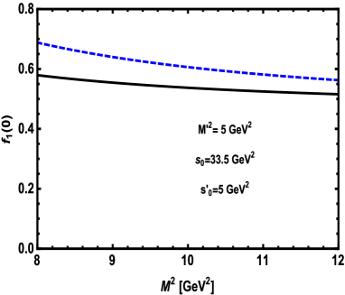
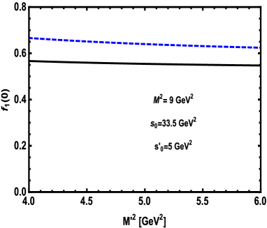
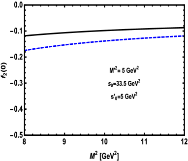
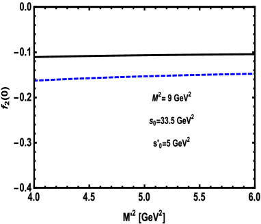
The continuum thresholds are not entirely capricious but they depend on the energy of the first excited states in the initial and final channels with the same quantum numbers as the interpolating currents. From numerical analysis, the working intervals are obtained as $s_{0}=(32.0\pm 1.5)~{}GeV^{2}$ and $s^{\prime}_{0}=(5.0\pm 0.5)~{}GeV^{2}$ for the continuum thresholds. The Borel mass parameters are restricted by requirements that, not only the contributions of the higher states and continuum are sufficiently suppressed but also the contributions of the higher dimensional operators are small. These conditions lead to the intervals $8~{}GeV^{2}\leq M^{2}\leq 12~{}GeV^{2}$ and $4~{}GeV^{2}\leq M^{2}\leq 6~{}GeV^{2}$. In order to see how our results depend on the Borel parameters, we present the dependence of the form factors $f_{1}(0)$ and $f_{2}(0)$, at fixed values of the continuum thresholds, on these parameters in Figs. 1 and 2. In these figures, the solid lines stand for the nuclear matter results and dashed lines for those of vacuum. From these figures we see that not only the form factors demonstrate good stabilities with respect to the variations of Borel parameters in their working regions, but the results obtained in the nuclear medium differ considerably with those of the vacuum.

Refer to caption Refer to caption
Figure 1: Left panel: the form factor $f_{1}(0)$ versus $M^{2}$ in nuclear matter (solid line) and vacuum (dashed line). Right panel: the form factor $f_{1}(0)$ versus $M^{\prime 2}$ in nuclear matter (solid line) and vacuum (dashed line).
Refer to caption Refer to caption
Figure 2: The same as figure $1$ but for $f_{2}(0)$ form factor.
Refer to caption Refer to caption
Figure 3: The dependence of the form factors $f_{1}(q^{2})$ (left panel) and $f_{2}(q^{2})$ (right panel) on $q^{2}$ in nuclear matter (solid line) and vacuum (dashed line).

Having determined the working regions for the continuum thresholds and Borel mass parameters, we proceed to find the behaviors of the form factors in terms of $q^{2}$ . Our analysis shows that the form factors are well fitted to the following function:

$$f_{i}(q^{2})=\frac{f_{i}(0)}{1+\alpha\hat{q}+\beta\hat{q}^{2}+\gamma\hat{q}^{3}+\lambda\hat{q}^{4}},$$ (29)

where $\hat{q}=q^{2}/m^{2}_{B_{q}}$ and the numerical values for the parameters $f_{i}(0)$, $\alpha$, $\beta$, $\gamma$ and $\lambda$ are presented in tables 2 and 3 for nuclear matter and vacuum, respectively. From these tables we see that although the central values of the form factors at $q^{2}=0$ seem to be considerably different in medium and vacuum, considering the errors roughly kills these differences. The errors in the results belong to the uncertainties in determination of the working regions for the auxiliary parameters as well as the errors in the other input parameters.
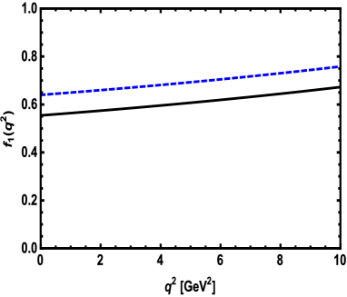
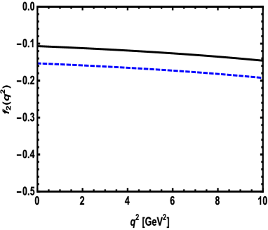
$f(0)$ $\alpha$ $\beta$ $\gamma$ $\lambda$
$f_{1}$ $0.55\pm 0.06$ $-0.48$ $-0.036$ $0.008$ $0.007$
$f_{2}$ $-0.11\pm 0.01$ $-0.67$ $-0.247$ $0.006$ $0.079$
Table 2: The numerical values for the parameters $f_{i}(0)$, $\alpha$, $\beta$, $\gamma$ and $\lambda$ in nuclear matter.
$f(0)$ $\alpha$ $\beta$ $\gamma$ $\lambda$
$f_{1}$ $0.64\pm 0.07$ $-0.41$ $-0.057$ $0.002$ $0.006$
$f_{2}$ $-0.15\pm 0.02$ $-0.47$ $-0.266$ $-0.085$ $0.023$
Table 3: The numerical values for the parameters $f_{i}(0)$, $\alpha$, $\beta$, $\gamma$ and $\lambda$ in vacuum.

We present the dependence of $f_{1}(q^{2})$ and $f_{2}(q^{2})$ on $q^{2}$ at average values of the Borel mass parameters and continuum thresholds in figure 3. From this figure we also see that, as far as the central values are concerned, the nuclear medium affect the $q^{2}$ dependencies of the form factors considerably.

The next step is to calculate the branching ratio of the process under consideration both in nuclear medium and vacuum for both $\ell=e,\mu$ and $\tau$, which are depicted in tables 4 and 5. For comparison, we also depict the existing experimental data. From these tables we obtain that the nuclear medium suppresses the values of branching ratios with amount of roughly 50% for all lepton channels when the central values are considered. It is also seen that the errors can not kill the differences between the medium and vacuum predictions in the case of branching fractions. The results of vacuum sum rules are consistent with the experimental data [27] for all lepton channels within the errors.

$Br$ $B^{+}\rightarrow\overline{D}^{0}\ell^{+}\nu_{\ell}$ $B^{+}\rightarrow\overline{D}^{0}\tau^{+}\nu_{\tau}$
Nuclear matter ($1.04\pm 0.29$)$\times 10^{-2}$ ($0.48\pm 0.13$)$\times 10^{-2}$
Table 4: The branching ratios in nuclear matter.
$Br$ $B^{+}\rightarrow\overline{D}^{0}\ell^{+}\nu_{\ell}$ $B^{+}\rightarrow\overline{D}^{0}\tau^{+}\nu_{\tau}$
Vacuum ($2.03\pm 0.57$) $\times 10^{-2}$ ($0.92\pm 0.26$) $\times 10^{-2}$
PDG [27] ($2.27\pm 0.11$)$\times 10^{-2}$ ($0.77\pm 0.25$)$\times 10^{-2}$
Table 5: The branching ratios in vacuum together with the experimental data.

At the end of this section, we would like to calculate the ratio of branching fractions in $\tau$ to $\ell=\mu,e$ channels, i.e.

$\displaystyle{\cal R}(D)=\frac{{\cal B}(B^{+}\rightarrow\overline{D}^{0}\tau^{+}\nu_{\tau})}{{\cal B}(B^{+}\rightarrow\overline{D}^{0}\ell^{+}\nu_{\ell})},$ (30)

for both the nuclear medium and vacuum. We obtain the value ${\cal R}(D)=0.461\pm 0.009$ for the nuclear medium which is roughly the same with the vacuum value ${\cal R}(D)=0.453\pm 0.009$ within the errors.

We conclude that although the nuclear medium effects cause considerable shifts in the central values of the form factors, considering the errors roughly kills these differences. In the case of branching ratios we see considerable differences between the medium and vacuum predictions for all lepton channels, which can not be killed by the errors of the form factors. This can be attributed to the shifts in the masses of the participating mesons due to the nuclear medium. The ratio of branching fractions in $\tau$ to $\ell=\mu,e$ channel remains roughly unchanged both in medium and vacuum. This ratio and other quantities in nuclear medium considered in the present work can be checked in future in-medium experiments.

4 Acknowledgement

This work has been supported in part by the Scientific and Technological Research Council of Turkey (TUBITAK) under the research project 114F018.

References

  • [1] J. P. Lees et al. (BABAR Collaboration), Phys. Rev. Lett. 109, 101802 (2012).
  • [2] P. Biancofiore, P. Colangelo, F. De Fazio, Phys. Rev. D 87, 074010 (2013).
  • [3] S. Fajfer, J. F. Kamenik and I. Nisandzic, Phys. Rev. D 85, 094025 (2012).
  • [4] S. Fajfer, J. F. Kamenik, I. Nisandzic and J. Zupan, Phys. Rev. Lett. 109, 161801 (2012).
  • [5] A. Crivellin, C. Greub and A. Kokulu, Phys. Rev. D 86, 054014 (2012).
  • [6] A. Datta, M. Duraisamy and D. Ghosh, Phys. Rev. D 86, 034027 (2012).
  • [7] D. Becirevic, N. Kosnik and A. Tayduganov, Phys. Lett. B 716, 208 (2012).
  • [8] D. Becirevic, N. Kosnik and A. Tayduganov, PoS ConfinementX, 244 (2012).
  • [9] A. Celis, M. Jung, X. -Q. Li and A. Pich, JHEP 1301, 054 (2013).
  • [10] D. Choudhury, D. K. Ghosh and A. Kundu, Phys. Rev. D 86, 114037 (2012).
  • [11] M. Tanaka and R. Watanabe, Phys. Rev. D 87, 034028 (2013).
  • [12] A. Bhol, EPL, 106, 31001 (2014).
  • [13] A. Hayashigaki, Phys. Lett. B 487, 96 (2000).
  • [14] T. Hilger, R. Thomas, B. KΓ€mpfer, Phys. Rev. C 79, 025202 (2009).
  • [15] T. Hilger, B. KΓ€mpfer, Nucl. Phys. Proc. Suppl. 207-208, 277 (2010).
  • [16] Z.-G. Wang, T. Huang, Phys. Rev. C 84, 048201 (2011).
  • [17] K. Azizi, N. Er, H. Sundu, Eur. Phys. J. C 74, 3021 (2014).
  • [18] E. Fioravanti, arXiv:1206.2214.
  • [19] B. Friman et al, β€œThe CBM physics book: Compressed Baryonic Matter in Laboratory Experiments”, Springer Heidelberg.
  • [20] http://www.gsi.de/fair/experiments/CBM/index e.html.
  • [21] http://www-panda.gsi.de/auto/phy/ home.htm.
  • [22] T. D. Cohen, R. J. Furnstahl, D. K. Griegel, X. Jin, Prog. Part. Nucl. Phys. 35, 221 (1995).
  • [23] L. J. Reinders, H. Rubinstein, S. Yazaki, Phys. Rep. 127, 1 (1985).
  • [24] X. Jin, T. D. Cohen, R. J. Furnstahl, and D. K. Griegel, Phys. Rev. C 47, 2882 (1993).
  • [25] X. Jin, M. Nielsen, T. D. Cohen, R. J. Furnstahl, D. K. Griegel, Phys. Rev. C 49, 464 (1994).
  • [26] T. D. Cohen, R. J. Furnstahl and D. K. Griegel, Phys. Rev. C 45, 1881 (1992).
  • [27] J. Beringer et al., Particle Data Group, Phys. Rev. D 86, 010001 (2012).