Computing Hasse–Witt matrices of hyperelliptic curves in average polynomial time, II

Abstract.

We present an algorithm that computes the Hasse–Witt matrix of given hyperelliptic curve over $\mathbb{Q}$ at all primes of good reduction up to a given bound $N$. It is simpler and faster than the previous algorithm developed by the authors.

1. Introduction

Let $C/\mathbb{Q}$ be a (smooth projective) hyperelliptic curve of genus $g$ defined by an affine equation of the form $y^{2}=f(x)$, with $f=\sum_{i}f_{i}x^{i}\in\mathbb{Z}[x]$ squarefree. Primes $p$ for which the reduced equation $y^{2}=f(x)\bmod p$ defines a hyperelliptic curve $C_{p}/\mathbb{F}_{p}$ of genus $g$ are primes of good reduction (for the equation $y^{2}=f(x)$). For each such prime $p$, the Hasse–Witt matrix (or Cartier–Manin matrix) of $C_{p}$ is the $g\times g$ matrix $W_{p}=[w_{ij}]$ over $\mathbb{Z}/p\mathbb{Z}$ with entries

$$w_{ij}=f^{(p-1)/2}_{pi-j}\bmod p\qquad(1\leq i,j\leq g),$$

where $f^{n}_{k}$ denotes the coefficient of $x^{k}$ in $f(x)^{n}$; see [14, 23] for details. The matrix $W_{p}$ depends on the equation $y^{2}=f(x)\bmod p$ for the curve $C_{p}$, but its conjugacy class, and in particular, its characteristic polynomial, is an invariant of the function field of $C_{p}$.

The Hasse–Witt matrix $W_{p}$ is closely related to the zeta function

(1) $$Z_{p}(T):=\exp\left(\sum_{k=1}^{\infty}\frac{\#C_{p}(\mathbb{F}_{p^{k}})}{k}T^{k}\right)=\frac{L_{p}(T)}{(1-T)(1-pT)}.$$

Indeed, the numerator $L_{p}\in\mathbb{Z}[T]$ satisfies

$$L_{p}(T)\equiv\det(I-TW_{p})\pmod{p},$$

and we also have

$$\chi_{p}(T)\equiv(-1)^{g}T^{g}\det(W_{p}-TI)\pmod{p},$$

where $\chi_{p}(T)$ denotes the characteristic polynomial of the Frobenius endomorphism of the Jacobian of $C_{p}$. In particular, the trace of $W_{p}$ is equal to the trace of Frobenius modulo $p$, and for $p>16g^{2}$ the Riemann Hypothesis for curves implies that this relationship uniquely determines the trace of Frobenius.

In this paper we present an algorithm that takes as input the polynomial $f(x)$ and an integer $N>1$, and simultaneously computes $W_{p}$ for all primes $p\leq N$ of good reduction. Our main result is the complexity bound given in Theorem 1.1 below; the details of the algorithm are given in §4.

All time complexity bounds refer to bit complexity. We denote by $\operatorname{\mathsf{M}}(s)$ the time needed to multiply $s$-bit integers; we may take $\operatorname{\mathsf{M}}(s)=O(s\,(\log s)^{1+o(1)})$ (see [17, 4], or [9] for recent improvements). We assume throughout that $\operatorname{\mathsf{M}}(s)/(s\log s)$ is increasing, and that the space complexity of $s$-bit integer multiplication is $O(s)$.

Theorem 1.1.

Assume that $g\log g=O(\log N)$ and that $\log\max_{i}|f_{i}|=O(\log N)$. The algorithm ComputeHasseWittMatrices computes $W_{p}$ for all primes $p\leq N$ of good reduction in $O(g^{3}\operatorname{\mathsf{M}}(N\log N)\log N)$ time and $O(g^{2}N)$ space.

The average running time of ComputeHasseWittMatrices per prime $p\leq N$ is

$$O(g^{3}(\log p)^{4+o(1)}),$$

which is polynomial in $g\log p$, the bit-size of the equation defining $C_{p}$. While it is known that one can compute the characteristic polynomial of $W_{p}$ for any particular prime $p$ in time polynomial in $\log p$ (the Schoof–Pila algorithm [18, 16]), or polynomial in $g$ (Kedlaya’s algorithm [12], for example), we are aware of no algorithm that can compute even the trace of $W_{p}$ in time that is polynomial in $g\log p$.

The algorithm presented here improves the previous algorithm given by the authors in [10], which was in turn based on the approach introduced in [8]. The new algorithm is easier to describe and implement, and it is significantly faster. Asymptotically we gain a factor of $g^{2}$ in the running time: one factor of $g$ arises from genuine algorithmic improvements in the present paper, and another factor of $g$ follows from unrelated recent work on the theoretical complexity of integer matrix multiplication [11]. The new algorithm also uses less memory by a significant constant factor. Tables 1 and  2 in §7 give performance comparisons in genus 2 and 3, where the the new algorithm is already up to 8 times faster. Compared to previous methods for solving this problem (i.e., prior to [8]), the new algorithm is dramatically faster, with more than a 300-fold speed advantage for $N=2^{30}$; see Table 3. Performance results for hyperelliptic curves of genus $g\leq 10$ can be found in Table 4.

In addition to the average polynomial-time algorithm, we give an $O(g^{2}p\operatorname{\mathsf{M}}(\log p))$ algorithm to compute $W_{p}$ for a single prime $p\geq g$. While the dependence on $p$ is not asymptotically competitive with existing algorithms, it is easy to implement, and uses very little memory. The small constant factors in its complexity make it a good choice for small to medium values of $p$; see Table 5.

We also introduce techniques that may be of interest beyond the scope of our algorithmic applications. In particular, we show that the matrix $W_{p}$ for a given curve may be derived from knowledge of just the first row of the matrices $W_{p}$ corresponding to $g$ isomorphic curves. Algorithmically, this has the advantage that we never need to go beyond the coefficient of $x^{p-1}$ in the expansion of $f(x)^{((p-1)/2)}$ in order to compute $W_{p}$.

2. Recurrence relations

As above, let $C/\mathbb{Q}$ be a hyperelliptic curve of genus $g$. We may assume without loss of generality that $C$ is defined by an equation of the form

$$y^{2}=f(x)=\sum_{i=c}^{d}f_{i}x^{i}\qquad(f_{i}\in\mathbb{Z})$$

with $c\in\{0,1\}$, $d\in\{2g+1,2g+2\}$ and $f_{c}f_{d}\neq 0$ (we have $c\leq 1$ because $f$ is squarefree). It is convenient to normalize by taking $h(x):=f(x)/x^{c}$ and $r:=d-c$. Then

$$h(x)=\sum_{i=0}^{r}h_{i}x^{i}$$

where $h_{i}=f_{i+c}$ for $i=0,\ldots,r$, and $h_{0}h_{r}\neq 0$.

We now derive a recurrence for the coefficients $h^{n}_{k}$ of $h^{n}$, following the strategy of Bostan–Gaudry–Schost [1, §8]. The identities

$$h^{n+1}=h\cdot h^{n}\qquad\text{and}\qquad(h^{n+1})^{\prime}=(n+1)h^{\prime}\cdot h^{n}$$

yield the relations

$$h_{k}^{n+1}=\sum_{j=0}^{r}h_{j}h_{k-j}^{n}\qquad\text{and}\qquad kh_{k}^{n+1}=(n+1)\sum_{j=0}^{r}jh_{j}h_{k-j}^{n}.$$

Subtracting $k$ times the first relation from the second and solving for $h^{n}_{k}$ yields the recurrence

(2) $$h^{n}_{k}=\frac{1}{kh_{0}}\sum_{j=1}^{r}((n+1)j-k)h_{j}h^{n}_{k-j},$$

which expresses $h^{n}_{k}$ in terms of the previous $r$ coefficients $h^{n}_{k-1},\ldots,h^{n}_{k-r}$, for all $k>0$.

The recurrence may be written in matrix form as follows. Define the integer row vector

$$v_{k}^{n}:=[h^{n}_{k-r+1},\ldots,h^{n}_{k}]\in\mathbb{Z}^{r}.$$

Then

$$v^{n}_{k}=\frac{1}{kh_{0}}v^{n}_{k-1}M^{n}_{k},$$

where

(3) $$M^{n}_{k}:=\begin{bmatrix}0&\cdots&0&((n+1)r-k)h_{r}\\ kh_{0}&\cdots&0&((n+1)(r-1)-k)h_{r-1}\\ \vdots&\ddots&\vdots&\vdots\\ 0&\cdots&kh_{0}&(n+1-k)h_{1}\end{bmatrix}.$$

Iterating the recurrence, we obtain an explicit formula for the $m$th term, for any $m\geq 0$:

$$v^{n}_{m}=\frac{1}{(h_{0})^{m}m!}v^{n}_{0}M^{n}_{1}\cdots M^{n}_{m}.$$

Since the initial vector is simply $v^{n}_{0}=[0,\ldots,0,(h_{0})^{n}]$, we may rewrite this as

(4) $$v^{n}_{m}=\frac{1}{(h_{0})^{m-n}m!}V_{0}M^{n}_{1}\cdots M^{n}_{m},$$

where

$$V_{0}:=[0,\ldots,0,1]\in\mathbb{Z}^{r}.$$

Everything discussed so far holds over $\mathbb{Z}$. Now consider a prime $p$ of good reduction that does not divide $h_{0}$, and let $W_{p}$ be the Hasse–Witt matrix of $y^{2}=f(x)\bmod p$, as in §1. Write $W_{p}^{i}$ for the $i$th row of $W_{p}$. Specializing the above discussion to $n:=(p-1)/2$, the entries of $W_{p}^{i}$ are given by $w_{ij}=f^{n}_{pi-j}=h^{n}_{pi-j-cn}\bmod p$ for $j=1,\ldots,g$. These are the last $g$ entries, in reversed order, of the vector $v^{n}_{pi-cn-1}\bmod p$, which by (4) is equal to

(5) $$\frac{1}{(h_{0})^{(pi-cn-1)-n}(pi-cn-1)!}V_{0}M^{n}_{1}\cdots M^{n}_{pi-cn-1}\pmod{p}.$$

Remark 2.1.

Bostan, Gaudry and Schost [1] used a formula essentially equivalent to (5) to compute $W_{p}$, for a single prime $p$. Their innovation was to evaluate the matrix product using an improvement of the Chudnovsky–Chudnovsky method, leading to an overall complexity bound of $g^{O(1)}p^{1/2+o(1)}$ for computing $W_{p}$.

Remark 2.2.

The power of $p$ dividing the denominator $(pi-cn-1)!$ in (5) is at least $p^{i-1}$. In particular, if $i\geq 2$, the denominator is divisible by $p$. Thus, to compute the second and subsequent rows of $W_{p}$, the algorithm in [1] artificially lifts the input polynomial $f\in\mathbb{F}_{p}[x]$ to $(\mathbb{Z}/p^{\lambda}\mathbb{Z})[x]$ for a suitable $\lambda\geq 2$, and then works modulo $p^{\lambda}$ throughout the computation, reducing modulo $p$ at the end. In this paper we compute $W_{p}$ by computing the first row of $g$ conjugate Hasse–Witt matrices (as explained in §5), so we can work modulo $p$ everywhere.

We now focus on $W_{p}^{1}$, the first row of $W_{p}$. Taking $i=1$ in (5) and putting $e:=2-c$, we find that $W_{p}^{1}$ is given by the last $g$ entries of

(6) $$v^{n}_{en}\equiv\frac{1}{(h_{0})^{n(e-1)}(en)!}V_{0}M^{n}_{1}\cdots M^{n}_{en}\pmod{p}.$$

To compute $W_{p}^{1}$, it suffices to evaluate the vector-matrix product $V_{0}M^{n}_{1}\cdots M^{n}_{en}$ modulo $p$, since, having assumed $p\centernot|h_{0}$, the denominator $(h_{0})^{n(e-1)}(en)!$ is not divisible by $p$ (note that $e\in\{1,2\}$, so $en$ is at most $p-1$).

Remark 2.3.

The quantity $(h_{0})^{n}=(h_{0})^{(p-1)/2}$ is just the Legendre symbol $(h_{0}/p)=\pm 1$, and the denominator $(h_{0}/p)^{e-1}(en)!$ is always a fourth root of unity modulo $p$. Indeed, if $e=2$ then $(en)!=(p-1)!\equiv-1\pmod{p}$, by Wilson’s theorem; if $e=1$ then it is well known that $(en)!=((p-1)/2)!$ is a fourth root of unity modulo $p$. However, we know of no easy way to determine which fourth root of unity occurs. For example, if $p>3$ and $p\equiv 3\pmod{4}$, then $((p-1)/2)!\equiv\pm 1\pmod{p}$, where the sign depends on the class number of $\mathbb{Q}(\sqrt{-p})$ modulo $4$; see [15].

To evaluate (6) simultaneously for many primes, a crucial observation is that the matrix $M_{k}^{n}$ becomes “independent of $n$” after reduction modulo $p=2n+1$. More precisely, we have $2(n+1)=1\pmod{p}$, so $2M_{k}^{n}\equiv M_{k}\pmod{p}$ where

(7) $$M_{k}:=\begin{bmatrix}0&\cdots&0&(r-2k)h_{r}\\ 2kh_{0}&\cdots&0&(r-1-2k)h_{r-1}\\ \vdots&\ddots&\vdots&\vdots\\ 0&\cdots&2kh_{0}&(1-2k)h_{1}\end{bmatrix}.$$

Note that $M_{k}$ is defined over $\mathbb{Z}$, and, unlike $M^{n}_{k}$, it is independent of $p$. Multiplying (6) by $2^{en}$ yields the following lemma.

Lemma 2.4.

The first row $W_{p}^{1}$ of $W_{p}$ consists of the last $g$ entries of the vector

(8) $$\frac{\left(\frac{2}{p}\right)^{e}}{\left(\frac{h_{0}}{p}\right)^{e-1}(en)!}V_{0}M_{1}\cdots M_{en}\pmod{p}.$$

In order to unify the indexing for the cases $e=1$ and $e=2$ we now define

$$M^{\prime}_{k}:=\begin{cases}M_{k}&e=1,\\ M_{2k-1}M_{2k}&e=2.\end{cases}$$

Then (8) becomes

(9) $$\frac{\left(\frac{2}{p}\right)^{e}}{\left(\frac{h_{0}}{p}\right)^{e-1}(en)!}V_{0}M^{\prime}_{1}\cdots M^{\prime}_{n}\pmod{p}.$$

In the next section we will recall how to use the accumulating remainder tree algorithm to evaluate the product $V_{0}M^{\prime}_{1}\cdots M^{\prime}_{n}\pmod{p}$ for many primes $p$ simultaneously.

Remark 2.5.

The key difference between this approach and that of [10] is that here we express $v^{n}_{k}$ in terms of $v^{n}_{k-1}$, instead of expressing $v^{k}_{2k}$ in terms of $v^{k-1}_{2k-2}$. In the terminology of [8], we have replaced “reduction towards zero” by “horizontal reduction”. In both cases, the aim is to obtain recurrences whose defining matrices are independent of $p$, so that the machinery of accumulating remainder trees can be applied. In the original “reduction towards zero” method of [10], the desired independence follows from the choice of indexing, i.e., because the superscript and subscript in $v^{k}_{2k}$ do not depend on $p$. In the new method, the superscript in $v^{n}_{k}$ does depend on $p$, but after reduction modulo $p$ the recurrence matrices turn out to be independent of $p$ anyway. The new method may also be viewed as a special case of (and was inspired by) the “generic prime” device introduced in [7]; see for example the proof of [7, Prop. 4.6].

Computationally, the new approach has two main advantages. First, the matrices $M_{k}$ are simpler, sparser, and have smaller coefficients than those in [10]. In fact, the formula for $M_{k}$ in [10] was so complicated that even for genus $2$ we did not write it out explicitly in the paper. Second, as pointed out earlier, none of the denominators $kh_{0}$ used to compute the first row of $W_{p}$ are divisible by $p$, so we can work modulo $p$ throughout; in [10] we needed to work modulo a large power of $p$ (at least $p^{g}$) in order to handle powers of $p$ appearing in the denominators.

3. Accumulating remainder trees

In this section we recall how the accumulating remainder tree algorithm works and sharpen some of the complexity bounds given in [10].

We follow the notation and framework of [10, §4]. Let $b\geq 2$ and let $m_{1},\ldots,m_{b-1}$ be a sequence of positive integer moduli. Let $A_{0},\ldots,A_{b-2}$ be a sequence of $r\times r$ integer matrices, and let $V$ be an $r$-dimensional integer row vector. We wish to compute the sequence of reduced row vectors $C_{1},\ldots,C_{b-1}$ defined by

$$C_{n}:=VA_{0}\cdots A_{n-1}\bmod m_{n}.$$

For convenience, we define $m_{0}:=1$, so $C_{0}$ is the zero vector, and we let $A_{b-1}$ be the identity matrix. (To apply this to the recurrences in §2, we let $V=V_{0}$ and $A_{k}=M^{\prime}_{k+1}$; note that the index $k$ is shifted by one place.)

In [10, §4] we gave an algorithm RemainderTree that efficiently computes the vectors $C_{1},\ldots,C_{b-1}$ simultaneously. For the reader’s convenience we now recall some details of this algorithm. As in [10], for simplicity we assume that $b=2^{\ell}$ is a power of $2$, though this is not strictly necessary.

We work with complete binary trees of depth $\ell$ with nodes indexed by pairs $(i,j)$ with $0\leq i\leq\ell$ and $0\leq j<2^{i}$. For each node we define the intermediate quantities

$$m_{i,j} :=m_{j2^{\ell-i}}m_{j2^{\ell-i}+1}\cdots m_{(j+1)2^{\ell-i}-1},$$

(10) $$A_{i,j} :=A_{j2^{\ell-i}}A_{j2^{\ell-i}+1}\cdots A_{(j+1)2^{\ell-i}-1},$$

$$C_{i,j} :=VA_{i,0}\cdots A_{i,j-1}\bmod m_{i,j}.$$

The values $m_{i,j}$ and $A_{i,j}$ may be viewed as nodes in a product tree, in which each node is the product of its children, with leaves $m_{j}=m_{\ell,j}$ and $A_{j}=A_{\ell,j}$, for $0\leq j<b$. Each vector $C_{i,j}$ is the product of $V$ and all the matrices $A_{i,j^{\prime}}$ that are nodes on the same level and to the left of $A_{i,j}$, reduced modulo $m_{i,j}$. The following algorithm, copied verbatim from [10], computes the target values $C_{j}=C_{\ell,j}$.

Algorithm RemainderTree

Given $V,A_{0},\ldots,A_{b-1}$, $m_{0},\ldots,m_{b-1}$, with $b=2^{\ell}$, compute $m_{i,j},A_{i,j}$, $C_{i,j}$ as follows:

1. Set $m_{\ell,j}=m_{j}$ and $A_{\ell,j}=A_{j}$, for $0\leq j<b$.

2. For $i$ from $\ell-1$ down to 1:
   For For $0\leq j<2^{i}$, set $m_{i,j}=m_{i+1,2j}m_{i+1,2j+1}$ and $A_{i,j}=A_{i+1,2j}A_{i+1,2j+1}$.

3. Set $C_{0,0}=V\bmod m_{0,0}$ and then for $i$ from 1 to $\ell$:
   Set For $0\leq j<2^{i}$ set $C_{i,j}=\begin{cases}C_{i-1,\lfloor j/2\rfloor}\bmod m_{i,j}\qquad&\text{if $j$ is even,}\\ C_{i-1,\lfloor j/2\rfloor}A_{i,j-1}\bmod m_{i,j}&\text{if $j$ is odd.}\\ \end{cases}$

A complexity analysis of this algorithm was given in [10, Theorem 4.1], closely following the argument of [8, Prop. 4]. The analysis assumed that classical matrix multiplication was used to compute the products $A_{i+1,2j}A_{i+1,2j+1}$ in step 2. More precisely, defining $\operatorname{\mathsf{M}}_{r}(s)$ to be the cost (bit complexity) of multiplying $r\times r$ matrices with $s$-bit integer entries, it was assumed that $\operatorname{\mathsf{M}}_{r}(s)=O(r^{3}\operatorname{\mathsf{M}}(s))$. Of course, this can be improved to $\operatorname{\mathsf{M}}_{r}(s)=O(r^{\omega}\operatorname{\mathsf{M}}(s))$, where $\omega\leq 3$ is any feasible exponent for matrix multiplication [22, Ch. 12]. For example, we can take $\omega=\log 7/\log 2\approx 2.807$ using Strassen’s algorithm.

However, it was pointed out in [10] and [8] that one can do even better in practice, by reusing Fourier transforms of the matrix entries; heuristically this reduces the complexity to only $O(r^{2}\operatorname{\mathsf{M}}(s))$ when $s$ is large compared to $r$. Recently, a rigorous statement along these lines was established by van der Hoeven and the first author [11]. The following slightly weaker claim is enough for our purposes.

Lemma 3.1.

We have

$$\operatorname{\mathsf{M}}_{r}(s)=O(r^{2}\operatorname{\mathsf{M}}(s)+r^{\omega}s(\log\log s)^{2}),$$

uniformly for $r$ and $s$ in the region $r=O(s)$.

Proof.

According to [11, Prop. 4] (which depends on our running hypothesis that $\operatorname{\mathsf{M}}(s)/(s\log s)$ is increasing), in this region we have

$$\operatorname{\mathsf{M}}_{r}(s)=O(r^{2}\operatorname{\mathsf{M}}(s)+r^{\omega}(s/\log s)\operatorname{\mathsf{M}}(\log s)).$$

The desired bound follows, since certainly $\operatorname{\mathsf{M}}(n)=O(n\log^{2}n)$. ∎

Using this lemma, we can prove the following strengthening of [10, Theorem 4.1].

Theorem 3.2.

Let $B$ be an upper bound on the bit-size of $\prod_{j=0}^{b-1}m_{j}$, let $B^{\prime}$ be an upper bound on the bit-size of any entry of $V$, and let $H$ be an upper bound on the bit-size of any $m_{0},\ldots,m_{b-1}$ and any entry of $A_{0},\ldots,A_{b-1}$. Assume that $\log r=O(H)$ and that $r=O(\log b)$. The running time of the RemainderTree algorithm is

$$O(r^{2}\operatorname{\mathsf{M}}(B+bH)\log b+r\operatorname{\mathsf{M}}(B^{\prime})),$$

and its space complexity is

$$O(r^{2}(B+bH)\log b+rB^{\prime}).$$

This statement differs from [10, Theorem 4.1] in two ways: we have imposed the additional requirement that $r=O(\log b)$, and the $r^{3}\operatorname{\mathsf{M}}(B+bH)\log b$ term in the time complexity is improved to $r^{2}\operatorname{\mathsf{M}}(B+bH)\log b$ (we have also changed $h$ to $H$ to avoid a collision of notation).

Proof.

Let us first estimate the complexity of computing the $A_{i,j}$ tree. The entries of any product $A_{j_{1}}\cdots A_{j_{2}-1}$ have bit-size $O((j_{2}-j_{1})(H+\log r))=O((j_{2}-j_{1})H)$. Thus at level $\ell-i$ of the tree, each matrix product has cost

$$O(\operatorname{\mathsf{M}}_{r}(2^{i}H))=O(r^{2}\operatorname{\mathsf{M}}(2^{i}H)+r^{\omega}(2^{i}H)(\log\log 2^{i}H)^{2}),$$

by Lemma 3.1. There are $2^{\ell-i}$ such products at this level, whose total cost is

$$O(r^{2}\operatorname{\mathsf{M}}(bH)+r^{\omega}(bH)(\log\log bH)^{2}).$$

Since we assumed that $r=O(\log b)=O(\log bH)$, this is bounded by

$$O(r^{2}\operatorname{\mathsf{M}}(bH)+r^{2}(bh)(\log bH)^{\omega-2}(\log\log bH)^{2}).$$

But we may take $\omega<3$, and then certainly $(bH)(\log bH)^{\omega-2}(\log\log bH)^{2}=O(\operatorname{\mathsf{M}}(bH))$, again by the assumption that $\operatorname{\mathsf{M}}(s)/(s\log s)$ is increasing. The first term dominates, and we are left with the bound $O(r^{2}\operatorname{\mathsf{M}}(bH))$ for this level of the tree, and hence

$$O(r^{2}\operatorname{\mathsf{M}}(bH)\log b)$$

for the whole tree.

The rest of the argument is exactly the same as in [10] and [8]; we omit the details. ∎

In [10] we also gave an algorithm RemainderForest, which has the same input and output specifications as RemainderTree, but saves space by splitting the work into $2^{\kappa}$ subtrees, where $\kappa\in[0,\ell]$ is a parameter. (In [10] the parameter $\kappa$ was called $k$.) This is crucial for practical computations, as RemainderTree is extremely memory-intensive.

Theorem 3.2 leads to the following complexity bound for RemainderForest, improving Theorem 4.2 of [10]. We omit the proof, which is exactly the same as in [10], with obvious modifications to take account of Theorem 3.2.

Theorem 3.3.

Let $B$ be an upper bound on the bit-size of $\,\prod_{j=0}^{b-1}m_{j}$ such that $B/2^{\kappa}$ is an upper bound on the bit-size of $\prod_{j=st}^{st+t-1}m_{j}$ for all $s$, where $t:=2^{\ell-\kappa}$. Let $B^{\prime}$ be an upper bound on the bit-size of any entry of $V$, and let $H$ be an upper bound on the bit-size of any $m_{0},\ldots,m_{b-1}$ and any entry in $A_{0},\ldots,A_{b-1}$. Assume that $\log r=O(H)$ and that $r=O(\log b)$. The running time of the RemainderForest algorithm is

$$O(r^{2}\operatorname{\mathsf{M}}(B+bH)(\ell-\kappa)+2^{\kappa}r^{2}\operatorname{\mathsf{M}}(B)+r\operatorname{\mathsf{M}}(B^{\prime})),$$

and its space complexity is

$$O(2^{-\kappa}r^{2}(B+bH)(\ell-\kappa)+r(B+B^{\prime})).$$

4. Computing the first row

As above we work with a hyperelliptic curve $C/\mathbb{Q}$ of genus $g$ defined by $y^{2}=f(x)$, where $f(x)=\sum_{i=c}^{d}f_{i}x^{i}\in\mathbb{Z}[x]$ is squarefree and $f_{c}f_{d}\neq 0$. We define $h(x):=f(x)/x^{c}=\sum_{i=0}^{r}h_{i}x_{i}$ with $r:=d-c$ and put $e:=2-c\in\{1,2\}$, as in §2. We call a prime $p$ admissible if it is a prime of good reduction that does not divide $h_{0}$. The following algorithm uses (9) to compute $W_{p}^{1}$, the first row of the Hasse–Witt matrix $W_{p}$, simultaneously for admissible primes $p\leq N$.

Algorithm ComputeHasseWittFirstRows

Given an integer $N>1$ and a hyperelliptic curve $y^{2}=f(x)$ with $f(x),h(x)$, $r$, and $e$ as above, compute $W_{p}^{1}$ for all admissible primes $p\leq N$ as follows:

1. Let $\ell=\lceil\log_{2}N\rceil-1$ and initialize a sequence of moduli $m_{n}$ by

   $$m_{n}:=\begin{cases}p&\text{if $p=2n+1$ is an admissible prime in $[1,N]$},\\ 1&\text{otherwise},\end{cases}$$

   for all integers $n\in[1,2^{\ell})$.

2. Run RemainderForest with $b:=2^{\ell}$ and $\kappa:=\lceil 2\log_{2}\ell\rceil$ on inputs $V:=V_{0}$, $A_{k}:=M^{\prime}_{k+1}$, and $m_{k}$ with $k\in[0,b)$, where $V_{0}$ and $M^{\prime}_{k}$ are as defined in §2, to compute

   $$u_{n}:=V_{0}M^{\prime}_{1}\cdots M^{\prime}_{n}\bmod m_{n},$$

   for all integers $n\in[1,N/2)$. (One may set $A_{k}$ to the zero matrix for $k\geq N/2$).

3. Similarly, use RemainderForest to compute $\delta_{n}:=(en)!\bmod m_{n}$ for all $n\in[1,N/2)$.
   (For $e=2$ one can skip this step and simply set $\delta_{n}:=-1$; see Remark 2.3.)

4. For each admissible prime $p=2n+1\in[1,N]$ output the last $g$ entries of the vector

   $$\frac{\left(\frac{2}{p}\right)^{e}}{\left(\frac{h_{0}}{p}\right)^{e-1}\delta_{n}}u_{n}\bmod m_{n}$$

   in reverse order (this is the vector $W_{p}^{1}$).

Remark 4.1.

The bulk of the work in ComputeHasseWittFirstRows occurs in step 2. In the $e=2$ case, this step is about twice as expensive as the $e=1$ case, because there are twice as many matrices $M_{k}$; equivalently, the entries of $M^{\prime}_{k}$ are about twice as big. This suggests that it is advantageous to change variables, if possible, to achieve $e=1$. (Step 3 is more expensive when $e=1$, but the extra cost is negligible compared to the savings achieved in step 2.) This can be done if the curve has a rational Weierstrass point, by moving the Weierstrass point to $x=0$. In §6.1 we discuss further optimizations along these lines that may utilize up to $g+1$ rational Weierstrass points.

Theorem 4.2.

Assume that $g=O(\log N)$ and that $\log\max_{i}|f_{i}|=O(\log N)$. The algorithm ComputeHasseWittFirstRows runs in $O(g^{2}\operatorname{\mathsf{M}}(N\log N)\log N)$ time and $O(g^{2}N)$ space.

Proof.

Let us analyze the complexity of step 2, using Theorem 3.3. The prime number theorem implies that we may take $B=O(N)$, and the hypothesis on $B/2^{\kappa}$ follows easily (see the proof of [10, Theorem 1.1]). We also have $B^{\prime}=O(1)$ and

$$H=O(\log N+\log g+\log\max_{i}|h_{i}|)=O(\log N),$$

by the definition of the matrices $M^{\prime}_{k}$. The remaining hypotheses are satisfied since we have $r=O(g)=O(\log N)$. By Theorem 3.3 and our choice of $\kappa$, step 2 runs in time

$$O(g^{2}\operatorname{\mathsf{M}}(N\log N)\log N+(\log N)^{2}g^{2}\operatorname{\mathsf{M}}(N));$$

since $\operatorname{\mathsf{M}}(s)/(s\log s)$ is increasing, this simplifies to $O(g^{2}\operatorname{\mathsf{M}}(N\log N)\log N)$. The space complexity of step 2 is

$$O((\log N)^{-2}g^{2}(N\log N)\log N+gN)=O(g^{2}N).$$

The second invocation of RemainderForest (step 3) is certainly no more expensive than the first. The remaining steps such as enumerating primes and computing quadratic residue symbols take negligible time (see the proof of [10, Theorem 1.1]). ∎

Remark 4.3.

In practice, the parameter $\kappa$ is chosen based on empirical performance considerations, rather than strictly according to the formula given above.

Remark 4.4.

The $O(g^{2}N)$ space complexity of ComputeHasseWittFirstRows is larger than the $O(gN)$ size of its output. Most of this space can be reused in subsequent calls to ComputeHasseWittFirstRows, so we only need $O(g^{2}N)$ space to handle $g$ calls, as in algorithm ComputeHasseWittMatrices below; this allows us to obtain the $O(g^{2}N)$ space bound of Theorem 1.1.

For inadmissible primes $p$, ComputeHasseWittFirstRows does not yield any information about $W_{p}^{1}$. When $f_{0}=0$ every good prime is admissible (if $f_{0}=0$ and $p$ divides $h_{0}=f_{1}$ then $f(x)$ is not squarefree modulo $p$), but when $f_{0}\neq 0$ (the case $e=2-c=2$), there may be primes of good reduction that divide $f_{0}$ and are therefore inadmissible.

To compute $W_{p}^{1}$ at such primes, we must use an alternative algorithm. There are many possible choices, but we present here an algorithm that uses the framework developed in §2. The idea is to evaluate the product in (8) in the most naive way possible. To our knowledge, this simple algorithm has not been mentioned previously in the literature.

We first set some notation. Let $\bar{f}\in\mathbb{F}_{p}[x]$ denote a polynomial for which $y^{2}=\bar{f}(x)$ defines a hyperelliptic $C_{p}/\mathbb{F}_{p}$ of genus $g$ (so $\bar{f}$ is squarefree of degree $\bar{d}=2g+1$ or $\bar{d}=2g+2$), let $\bar{c}$ be the least integer for which $\bar{f}_{\bar{c}}\neq 0$, and set $\bar{r}:=\bar{d}-\bar{c}$. (Note: in the case of interest, $\bar{f}=f\bmod p$, but $p$ divides $f_{0}\neq 0$, so $\bar{c}\neq c$). Now define $\bar{h}(x):=\sum_{i=0}^{\bar{r}}\bar{h}_{i}x^{i}=\bar{f}(x)/x^{\bar{c}}$ and $\bar{e}:=2-\bar{c}$. Let $n:=(p-1)/2$ as usual, and let $\bar{M}_{k}$ be the matrix over $\mathbb{F}_{p}$ defined in (7), with $h_{i}$ replaced by $\bar{h}_{i}$. The following algorithm uses Lemma 2.4 to compute the first row $W_{p}^{1}$ of the Hasse–Witt matrix of $C_{p}$.

Algorithm ComputeHasseWittFirstRow

Let $y^{2}=\bar{f}(x)$ be a hyperelliptic curve $C_{p}/\mathbb{F}_{p}$, with notation as above. Compute the first row $W_{p}^{1}$ of the Hasse–Witt matrix of $C_{p}$ as follows:

1. Initialize $u_{0}:=[0,\ldots,0,1]\in(\mathbb{F}_{p})^{r}$ and $\delta_{0}:=1\in\mathbb{F}_{p}$.

2. For $k$ from $1$ to $\bar{e}n$, compute $u_{k}:=u_{k-1}\bar{M}_{k}$ and $\delta_{k}:=\delta_{k-1}k$.

3. Output the last $g$ entries of the vector

   $$\frac{\left(\frac{2}{p}\right)^{\bar{e}}}{\left(\frac{\bar{h}_{0}}{p}\right)^{\bar{e}-1}\delta_{\bar{e}n}}u_{\bar{e}n}.$$

Theorem 4.5.

The algorithm ComputeHasseWittFirstRow runs in $O(gp\operatorname{\mathsf{M}}(\log p))$ time and uses $O(g\log p)$ space.

Proof.

Each matrix $\bar{M}_{k}$ has at most $2r-1=O(g)$ nonzero entries, each of which can be computed using $O(1)$ ring operations. Each iteration of step 2 uses $O(g\operatorname{\mathsf{M}}(\log p))$ bit operations, and the number of iterations is $O(p)$, yielding a total cost of $O(gp\operatorname{\mathsf{M}}(\log p))$ for step 2. The Legendre symbol and division in step 3 require at most $O(\log^{2}p)$ bit operations, which is negligible.

For the space bound, each $u_{k}$ and $\delta_{k}$ may overwrite $u_{k-1}$ and $\delta_{k-1}$, respectively. Each $\bar{M}_{k}$ requires just $O(g\log p)$ space and can be computed as needed and then discarded. ∎

The space bound in Theorem 4.5 is optimal; in fact, it matches the size of both the input and the output. In practice, this algorithm performs quite well for small to moderate $p$, primarily due its extremely small memory footprint; see §7 for performance details.

5. Hasse–Witt matrices of translated curves

In this section we fix a prime $p$ of good reduction for our hyperelliptic equation $y^{2}=f(x)$. For each integer $a$, let $W_{p}(a)=[w_{ij}(a)]$ denote the Hasse–Witt matrix of the translated curve $y^{2}=f(x+a)$ at $p$, and let $W_{p}^{1}(a)$ denote its first row. In this section we show that if we know $W_{p}^{1}(a_{i})$ for integers $a_{1},\ldots,a_{g}$ that are distinct modulo $p$, then we can deduce the entire Hasse–Witt matrix $W_{p}=[w_{ij}]$ of our original curve at $p$.

We first study how $W_{p}$ transforms under the translation $x\mapsto x+a$.

Theorem 5.1.

With notation as above we have

$$W_{p}(a)=T(a)W_{p}T(-a),$$

where $T(a):=[t_{ij}(a)]$ is the $g\times g$ upper triangular matrix with entries

$$t_{ij}(a):=\binom{j-1}{i-1}a^{j-i}\qquad(1\leq i,j\leq g).$$

Proof.

Let $F$ be the function field of the curve $y^{2}=f(x)$ over $\mathbb{F}_{p}$ (the fraction field of $\mathbb{F}_{p}[x,y]/(y^{2}-f(x)))$. The space $\Omega_{F}(0)$ of regular differentials on $F$ (as defined in [20, §1.5], for example) is a $g$-dimensional $\mathbb{F}_{p}$-vector space with basis $(\omega_{1},\ldots,\omega_{g})$, where

$$\omega_{i}:=\frac{x^{i-1}dx}{y}\qquad\qquad\,\,\,(1\leq i\leq g);$$

see [20, Ex. 4.6] and [23, Eq. 3]. It follows from [23, Prop. 2.2] that the Hasse–Witt matrix $W_{p}(a)$ has the form $SW_{p}S^{-1}$, where $S=[s_{ij}]$ is the change of basis matrix from the basis $(\omega_{1},\ldots,\omega_{g})$ to the basis $(\theta_{1},\ldots,\theta_{g})$, with

$$\theta_{j}:=\frac{(x+a)^{j-1}dx}{y}\qquad\,(1\leq j\leq g).$$

(Note that we have replaced the matrix $S^{(p)}=[s_{ij}^{p}]$ that appears in [23, Prop. 2.2] with $S=[s_{ij}]$ because we are working over $\mathbb{F}_{p}$ and therefore have $s_{ij}^{p}=s_{ij}$.) We then have

$$\theta_{j}=\frac{(x+a)^{j-1}dx}{y}=\sum_{i=1}^{j}\binom{j-1}{i-1}a^{j-i}\frac{x^{i-1}dx}{y}=\sum_{i=1}^{g}\binom{j-1}{i-1}a^{j-i}\omega_{i}=\sum_{i=1}^{g}t_{ij}(a)\omega_{i},$$

so $S=T(a)$, and $S^{-1}=T(a)^{-1}=T(-a)$. Thus $W_{p}(a)=SW_{p}S^{-1}=T(a)W_{p}T(-a)$. ∎

Now suppose that $p\geq g$ and that we have computed $W_{p}^{1}(a_{i})$ for integers $a_{1},\ldots,a_{g}$ that are distinct modulo $p$. Writing out the equation for the first row of $W_{p}(a_{i})=T(a_{i})W_{p}T(-a_{i})$ explicitly, we have

$$w_{1j}(a_{i})=\sum_{k=1}^{g}\sum_{\ell=1}^{g}t_{1k}(a_{i})w_{k\ell}t_{\ell j}(-a_{i})=\sum_{k=1}^{g}\sum_{\ell=1}^{j}\binom{j-1}{\ell-1}(-1)^{j-\ell}a_{i}^{k-1+j-\ell}w_{k\ell}.$$

As $i$ and $j$ range over $\{1,\ldots,g\}$, this may be regarded as a system of $g^{2}$ linear equations in the $g^{2}$ unknowns $w_{k\ell}$ over $\mathbb{F}_{p}$.

We claim that this system has a unique solution. Indeed, separating out the terms with $\ell=j$, we may write

$$w_{1j}(a_{i})=\bigl{(}w_{1j}+a_{i}w_{2j}+a_{i}^{2}w_{3j}+\cdots+a_{i}^{g-1}w_{gj}\bigr{)}+w_{j}(a_{i}),$$

where the last term

(11) $$w_{j}(a):=\sum_{k=1}^{g}\sum_{\ell=1}^{j-1}\binom{j-1}{\ell-1}(-1)^{j-\ell}a^{k-1+j-\ell}w_{k\ell}$$

depends only on $a$ and the first $j-1$ columns of $W_{p}$. Thus for each $j$ we have a system

(12) $$\begin{bmatrix}1&a_{1}&a_{1}^{2}&\cdots&a_{1}^{g-1}\\ 1&a_{2}&a_{2}^{2}&\cdots&a_{2}^{g-1}\\ \vdots&\vdots&\vdots&\vdots\\ 1&a_{g}&a_{g}^{2}&\cdots&a_{g}^{g-1}\\ \end{bmatrix}\begin{bmatrix}w_{1j}\\ w_{2j}\\ \vdots\\ w_{gj}\end{bmatrix}=\begin{bmatrix}w_{1j}(a_{1})-w_{j}(a_{1})\\ w_{1j}(a_{2})-w_{j}(a_{2})\\ \vdots\\ w_{1j}(a_{g})-w_{j}(a_{g})\end{bmatrix}.$$

The matrix on the left is a Vandermonde matrix $V(a_{1},\ldots,a_{g})$; it is non-singular because the $a_{i}$ are distinct in $\mathbb{F}_{p}$. Therefore for each $j=1,\ldots,g$ the system (12) determines the $j$th column of $W_{p}$ uniquely in terms of the $w_{1j}(a_{i})$ and the first $j-1$ columns of $W_{p}$. Given as input $w_{1j}(a_{i})$ for all $i$ and $j$, we may solve this system successively for $j=1,\ldots,g$ to determine all $g$ columns of $W_{p}$.

Example 5.2.

Consider the hyperelliptic curve

$$y^{2}=f(x)=2x^{8}+3x^{7}+5x^{6}+7x^{5}+11x^{4}+13x^{3}+17x^{2}+19x+23,$$

over the finite field $\mathbb{F}_{97}$, and let $a_{1}=0,a_{2}=1,a_{3}=2$. Computing the first rows of the Hasse–Witt matrices $W_{p}(0),W_{p}(1),W_{p}(2)$ yields

$$w_{11}(0)=\phantom{0}9,\quad w_{12}(0)=37,\quad w_{13}(0)=54,$$

$$w_{11}(1)=43,\quad w_{12}(1)=60,\quad w_{13}(1)=30,$$

$$w_{11}(2)=\phantom{0}5,\quad w_{12}(2)=70,\quad w_{13}(2)=84.$$

Solving the system

$$\begin{bmatrix}1&0&0\\ 1&1&1\\ 1&2&4\\ \end{bmatrix}\begin{bmatrix}w_{11}\\ w_{21}\\ w_{31}\end{bmatrix}=\begin{bmatrix}w_{11}(0)\\ w_{11}(1)\\ w_{11}(2)\\ \end{bmatrix}=\begin{bmatrix}9\\ 43\\ 5\end{bmatrix}$$

gives $w_{11}=9,w_{21}=70,w_{31}=61$, the first column of $W_{p}$. Using (11) to compute $w_{2}(0)=0$, $w_{2}(1)=54$, $w_{2}(2)=87$, we then solve

$$\begin{bmatrix}1&0&0\\ 1&1&1\\ 1&2&4\\ \end{bmatrix}\begin{bmatrix}w_{12}\\ w_{22}\\ w_{32}\end{bmatrix}=\begin{bmatrix}w_{12}(0)-w_{2}(0)\\ w_{12}(1)-w_{2}(1)\\ w_{12}(2)-w_{2}(2)\\ \end{bmatrix}=\begin{bmatrix}37\\ 6\\ 80\end{bmatrix}$$

to get the second column $w_{12}=37$, $w_{22}=62$, $w_{32}=4$. Finally, using (11) to compute $w_{3}(0)=0$, $w_{3}(1)=31$, $w_{3}(2)=88$ we solve

$$\begin{bmatrix}1&0&0\\ 1&1&1\\ 1&2&4\\ \end{bmatrix}\begin{bmatrix}w_{13}\\ w_{23}\\ w_{33}\end{bmatrix}=\begin{bmatrix}w_{13}(0)-w_{3}(0)\\ w_{13}(1)-w_{3}(1)\\ w_{13}(2)-w_{3}(2)\\ \end{bmatrix}=\begin{bmatrix}54\\ 96\\ 93\end{bmatrix}$$

to get the third column $w_{13}=54$, $w_{23}=16$, $w_{33}=26$, and we have

$$W_{p}=\begin{bmatrix}9&37&54\\ 70&62&16\\ 61&4&26\end{bmatrix},$$

which is the Hasse–Witt matrix of $y^{2}=f(x)$.

We now bound the complexity of this procedure. The bound given in the lemma below is likely not the best possible, but it suffices for our purposes here.

Lemma 5.3.

Given $W_{p}^{1}(a_{1}),\ldots,W_{p}^{1}(a_{g})$, we may compute $W_{p}$ in

$$O((g^{3}+g^{2}\log\log p)\operatorname{\mathsf{M}}(\log p))$$

time and $O(g^{2}\log p)$ space.

Proof.

We first invert the Vandermonde matrix $V(a_{1},\ldots,a_{g})$. This requires $O(g^{2})$ field operations in $\mathbb{F}_{p}$, by [2], or $O(g^{2}\operatorname{\mathsf{M}}(\log p)\log\log p)$ bit operations.

To compute $W_{p}$, we use the algorithm sketched above. More precisely, let us define $\beta_{j}(a):=\sum_{k=1}^{g}a^{k-1}w_{kj}$, so that

$$w_{j}(a_{i})=\sum_{\ell=1}^{j-1}\binom{j-1}{\ell-1}(-a_{i})^{j-\ell}\beta_{\ell}(a_{i}).$$

Having computed column $j-1$ of $W_{p}$, we may compute $\beta_{j-1}(a_{i})$ for all $i$, at a cost of $O(g^{2})$ ring operations in $\mathbb{F}_{p}$. We then use the formula above to compute $w_{j}(a_{i})$ for all $i$, again at a cost of $O(g^{2})$ ring operations. Finally we solve (12) for the $j$th column of $W_{p}$, using the known inverse of $V(a_{1},\ldots,a_{g})$, with $O(g^{2})$ ring operations. This procedure is repeated for $j=1,\ldots,g$, for a total of $O(g^{3})$ ring operations, or $O(g^{3}\operatorname{\mathsf{M}}(\log p))$ bit operations.

The space bound is clear; we only need space for $O(g^{2})$ elements of $\mathbb{F}_{p}$. ∎

6. Computing the whole matrix

In this section we assemble the various components we have developed to obtain an algorithm for computing the whole Hasse–Matrix matrix $W_{p}$. We begin with an algorithm that handles a single prime $p\geq g$.

Algorithm ComputeHasseWittMatrix

Given a hyperelliptic curve $y^{2}=f(x)$ over $\mathbb{F}_{p}$ of genus $g\leq p$, compute the Hasse–Witt matrix $W_{p}$ as follows:

1. For $g$ distinct $a_{i}\in\mathbb{F}_{p}$, compute $W_{p}^{1}(a_{i})$ by applying ComputeHasseWittFirstRow to the equation $y^{2}=f(x+a_{i})$.

2. Deduce $W_{p}$ from $W_{p}^{1}(a_{1}),\ldots,W_{p}^{1}(a_{g})$ using Lemma 5.3.

Theorem 6.1.

The algorithm ComputeHasseWittMatrix runs in $O(g^{2}p\operatorname{\mathsf{M}}(\log p))$ time and $O(g^{2}\log p)$ space.

Proof.

For each $i$, computing the polynomial $f(x+a_{i})$ costs $O(g^{2})$ ring operations in $\mathbb{F}_{p}$, and this is dominated by the $O(gp\operatorname{\mathsf{M}}(\log p))$ bit complexity of computing $W_{p}^{1}(a_{i})$ (Theorem 4.5), since $g\leq p$. Thus we can compute $W_{p}^{1}(a_{1}),\ldots,W_{p}^{1}(a_{g})$ in $O(g^{2}p\operatorname{\mathsf{M}}(\log p))$ time. By Lemma 5.3 we may deduce $W_{p}$ in time

$$O((g^{3}+g^{2}\log\log p)\operatorname{\mathsf{M}}(\log p))=O(g^{2}p\operatorname{\mathsf{M}}(\log p)).$$

The space bound follows immediately from the bounds in Theorem 4.5 and Lemma 5.3. ∎

Finally we arrive at ComputeHasseWittMatrices, which computes $W_{p}$ for all good primes $p\leq N$ by computing $W_{p}^{1}(a_{i})$ for $g$ chosen integers $a_{i}$ and all suitable primes $p\leq N$. We rely on ComputeHasseWittMatrix to fill in the values of $W_{p}$ at any good primes $p$ that are inadmissible for one of the translated curve $y^{2}=f(x+a_{i})$ or for which the $a_{i}$ are not distinct modulo $p$.

Algorithm ComputeHasseWittMatrices

Given a hyperelliptic curve $y^{2}=f(x)$ with $f\in\mathbb{Z}[x]$, and an integer $N>1$, compute the Hasse–Witt matrices $W_{p}$ for all primes $p\leq N$ of good reduction as follows:

1. For odd primes $p<g$ of good reduction compute $W_{p}$ directly from its definition by expanding $f(x)^{(p-1)/2}\bmod p$ and selecting the appropriate coefficients.

2. Choose $g$ distinct integers $a_{1},\ldots,a_{g}$ that are either roots of $f(x)$ or in the interval $[0,g)$. Let $\mathcal{S}$ be the set of primes $p\in[g,N]$ of good reduction that divide some $a_{i}-a_{j}$ or some nonzero $f(a_{i})$.

3. For primes $p\in\mathcal{S}$, use ComputeHasseWittMatrix to compute $W_{p}$.

4. Use ComputeHasseWittFirstRows to compute $W_{p}^{1}(a_{1}),\ldots,W_{p}^{1}(a_{g})$ for all primes $p\in[g,N]$ of good reduction that do not lie in $\mathcal{S}$. Then deduce $W_{p}$ for each such prime using Lemma 5.3.

Remark 6.2.

As in [10], the execution of the $g$ calls to ComputeHasseWittFirstRows in step 4 may be interleaved so that $W_{p}^{1}(a_{1}),\ldots,W_{p}^{1}(a_{g})$ are computed for batches of primes $p$ corresponding to subtrees of the remainder forest, and the computation of the matrices $W_{p}$ for these primes can then be completed batch by batch.

We now prove the main theorem announced in §1, which states that ComputeHasseWittMatrices runs in $O(g^{3}\operatorname{\mathsf{M}}(N\log N)\log N)$ time and $O(g^{2}N)$ space, under the hypotheses $g\log g=O(\log N)$ and $\log\max_{i}|f_{i}|=O(\log N)$.

In order to simplify the analysis, we assume that we always choose $a_{i}=i-1$ in step 2. (The complexity bounds of the theorem hold without this assumption, i.e., if we allow $a_{i}$ to be any root of $f(x)$, but we do not prove this.)

Proof of Theorem 1.1.

The time complexity of step 1 is $O(g\operatorname{\mathsf{M}}(\log N)+\operatorname{\mathsf{M}}(g^{2}\log g))$ for each prime; the first term covers the cost of reducing $f(x)$ modulo $p$, and the second covers the cost of computing $f(x)^{(p-1)/2}$ in the ring $\mathbb{F}_{p}[x]$. There are at most $g$ primes, so the overall cost is $O(g^{2}\operatorname{\mathsf{M}}(\log N)+g\operatorname{\mathsf{M}}(g^{2}\log g))$. The space complexity is $O(g^{2}\log g)$ for each prime, and also $O(g^{2}\log g)$ overall. Both bounds are dominated by the bounds given in the theorem.

The coefficient of $x^{j}$ in the translated polynomial $f^{(i)}(x):=f(x+a_{i})$ is $\sum_{k}\binom{k}{j}a^{k-j}f_{k}$, thus

$$\max_{j}|(f^{(i)})_{j}|\leq(2g+2)\binom{2g+2}{g+1}g^{2g+2}\max_{k}|f_{k}|,$$

and therefore $\log\max_{j}|(f^{(i)})_{j}|=O(g\log g+\log\max_{k}|f_{k}|)=O(\log N)$. In particular, the bit-size of $f(a_{i})$ is $O(\log N)$, so the number of primes that divide any particular $f(a_{i})$ is $O(\log N)$. Consequently, $|\mathcal{S}|=O(g\log N)$.

By Theorem 6.1, the total time spent in step 3 is $O((g\log N)(g^{2}N\operatorname{\mathsf{M}}(\log N)))$, which is dominated by $O(g^{3}\operatorname{\mathsf{M}}(N\log N)\log N)$. The space used in step 3 is negligible.

Finally, computing $W_{p}^{1}(a_{1}),\ldots,W_{p}^{1}(a_{g})$ for suitable primes $p\leq N$ in step 4 requires time $O(g^{3}\operatorname{\mathsf{M}}(N\log N)\log N)$ and space $O(g^{2}N)$, by Theorem 4.5. This dominates the contribution from Lemma 5.3, which is at most $O((N/\log N)(g^{3}+g^{2}\log\log N)\operatorname{\mathsf{M}}(\log N))$ over all primes. The space complexity of the latter is also negligible. ∎

6.1. Optimizations for curves with rational Weierstrass points

For hyperelliptic curves with one or more rational Weierstrass points the complexity of ComputeHasseWittMatrices can be improved by a significant constant factor. For curves with a rational Weierstrass point $P$, we can ensure that $d=2g+1$ by putting $P$ at infinity. This also ensures that every translated curve $y^{2}=f(x+a_{i})$ also has $d=2g+1$, and we get an overall speedup by a factor of at least

$$\left(\frac{2g+2}{2g+1}\right)^{2}$$

compared to the case where $C$ has no rational Weierstrass points, since we work with vectors and matrices of dimension $2g+1$ rather than $2g+2$. For example, the speedup is approximately $(6/5)^{2}=1.44$ for $g=2$ and $(8/7)^{2}\approx 1.31$ for $g=3$.

Alternatively, putting $P$ at zero and choosing $a_{1}=0$ speeds up the computation of $W_{p}^{1}(a_{1})$ by a factor of two (because we have half as many matrices $M_{k}$ to deal with), but it does not necessarily speed up the computation of $W_{p}^{1}(a_{2}),\ldots,W_{p}^{1}(a_{g})$. If we have just a single rational Weierstrass point we should put it at zero when $g\leq 2$, but otherwise we should put it at infinity.

When $C$ has more than one rational Weierstrass point we can get a further performance improvement by putting rational Weierstrass points at both zero and infinity and choosing $a_{1}=0$. If there are any other rational Weierstrass points, we should then choose $a_{2},\ldots,a_{g}$ to be the negations of the $x$-coordinates of any other rational Weierstrass points. Without loss of generality we may assume that these coordinates are all integral, since once we have $y^{2}=f(x)$ with a rational Weierstrass point at infinity, the polynomial $f(x)$ has odd degree and can be made monic (and integral) by scaling $x$ and $y$ appropriately. These changes may impact the size of the coefficients of $f$, but such changes are typically small, and may even be beneficial (in any case, for sufficiently large $N$ the benefit outweighs the cost).

For each $a_{i}$ for which $y^{2}=f(x+a_{i})$ has rational Weierstrass points at zero and infinity we get a speedup by a factor of

(13) $$2\left(\frac{g+1}{g}\right)^{2}$$

in the time to compute $W_{p}^{1}(a_{i})$, relative to the case where $y^{2}=f(x)$ has no rational Weierstrass points; we get a factor of $2$ because the number of matrices $M_{k}$ is halved, and then a factor of $((2g+2)/(2g))^{2}$ from the reduction in dimension of matrices and vectors. When $C$ has $g+1$ rational Weierstrass points we get a total speedup by the factor given in (13), relative to the case where there are no rational Weierstrass points. The speedup observed in practice is a bit better than this, as may be seen in Tables 1 and 2. This can be explained by the fact that the cost of matrix multiplication is actually super-quadratic at the lower levels of the accumulating remainder trees.

Remark 6.3.

The same speedup can be achieved when there are just $g$ rational Weierstrass points, by also computing the last row of $W_{p}$ and only using $g-1$ translated curves.

7. Performance results

We implemented our algorithms using the GNU C compiler (gcc version 4.8.2) and the GNU multiple precision arithmetic library (GMP version 6.0.0). The timings listed in the tables that follow were all obtained on a single core of an Intel Xeon E5-2697v2 CPU running at a fixed clock rate of 2.70GHz with 256 GB of RAM.

		$w=0$			$w=1$			$w=2$
$N$		hw1	hw2		hw1	hw2		hw1	hw2
$2^{14}$		0.8	0.2		0.5	0.1		0.3	0.1
$2^{15}$		2.6	0.6		1.2	0.3		0.6	0.2
$2^{16}$		5.8	1.6		3.2	0.8		1.6	0.4
$2^{17}$		14.0	4.1		8.1	2.2		4.1	1.0
$2^{18}$		33.1	9.5		20.4	5.1		9.7	2.3
$2^{19}$		81.3	21.8		49.6	12.1		23.5	5.3
$2^{20}$		$192$	51.3		$116$	28.2		56.4	12.6
$2^{21}$		$470$	$122$		$274$	66.7		$142$	29.0
$2^{22}$		$1\text{,}183$	$280$		$638$	$155$		$335$	67.6
$2^{23}$		$2\text{,}830$	$654$		$1\text{,}510$	$353$		$789$	$160$
$2^{24}$		$6\text{,}500$	$1\text{,}520$		$3\text{,}500$	$845$		$1\text{,}820$	$347$
$2^{25}$		$15\text{,}000$	$3\text{,}460$		$8\text{,}190$	$1\text{,}890$		$4\text{,}240$	$834$
$2^{26}$		$34\text{,}100$	$7\text{,}480$		$18\text{,}700$	$4\text{,}280$		$9\text{,}620$	$1\text{,}870$

Table 1. Comparison of old (hw1) and new (hw2) average polynomial-time algorithms for genus 2 curves over $\mathbb{Q}$ with $w$ rational Weierstrass points (times in CPU seconds).

		$w=0$			$w=1$			$w=2$			$w=3$
$N$		hw1	hw2		hw1	hw2		hw1	hw2		hw1	hw2
$2^{14}$		3.3	0.5		2.3	0.4		1.5	0.3		1.4	0.2
$2^{15}$		10.8	1.5		6.1	1.0		5.1	0.7		3.7	0.5
$2^{16}$		25.9	4.6		16.8	2.9		10.0	2.1		9.9	1.2
$2^{16}$		62.1	12.6		40.4	7.8		23.2	5.5		23.6	3.3
$2^{18}$		$147$	28.9		96.1	17.3		57.1	12.6		56.7	7.7
$2^{19}$		$347$	68.1		$230$	42.7		$141$	30.2		$139$	18.5
$2^{20}$		$878$	$156$		$544$	99.4		$326$	68.2		$329$	42.6
$2^{21}$		$1\text{,}950$	$363$		$1\text{,}280$	$231$		$792$	$161$		$782$	97.1
$2^{22}$		$4\text{,}500$	$841$		$3\text{,}130$	$528$		$1\text{,}840$	$370$		$1\text{,}820$	$225$
$2^{23}$		$10\text{,}700$	$1\text{,}920$		$7\text{,}370$	$1\text{,}260$		$4\text{,}380$	$859$		$4\text{,}330$	$533$
$2^{24}$		$24\text{,}300$	$4\text{,}360$		$16\text{,}800$	$2\text{,}830$		$10\text{,}200$	$2\text{,}010$		$9\text{,}960$	$1\text{,}200$
$2^{25}$		$60\text{,}400$	$9\text{,}910$		$39\text{,}000$	$6\text{,}220$		$23\text{,}800$	$4\text{,}430$		$2\text{,}320$	$2\text{,}710$
$2^{26}$		$128\text{,}000$	$21\text{,}000$		$83\text{,}900$	$13\text{,}700$		$53\text{,}400$	$9\text{,}930$		$53\text{,}100$	$5\text{,}980$

Table 2. Comparison of old (hw1) and new (hw2) average polynomial-time algorithms for genus 3 hyperelliptic curves over $\mathbb{Q}$ with $w$ rational Weierstrass points (times in CPU seconds).

		genus 2			genus 3
$N$		sj	hw2		hf	hw2
$2^{14}$		0.2	0.1		7.2	0.4
$2^{15}$		0.6	0.3		16.3	1.0
$2^{16}$		1.7	0.9		39.1	2.9
$2^{17}$		5.5	2.2		98.3	7.8
$2^{18}$		19.2	5.3		$255$.0	18.3
$2^{19}$		78.4	12.5		$695$.0	43.2
$2^{20}$		$271$.0	27.8		$1\text{,}950$.0	98.8
$2^{21}$		$1\text{,}120$.0	64.5		$5\text{,}600$.0	$229$.0
$2^{22}$		$2\text{,}820$.0	$155$.0		$16\text{,}700$.0	$537$.0
$2^{23}$		$9\text{,}840$.0	$357$.0		$51\text{,}200$.0	$1\text{,}240$.0
$2^{24}$		$31\text{,}900$.0	$823$.0		$158\text{,}000$.0	$2\text{,}800$.0
$2^{25}$		$105\text{,}000$.0	$1\text{,}890$.0		$501\text{,}000$.0	$6\text{,}280$.0
$2^{26}$		$349\text{,}000$.0	$4\text{,}250$.0		$1\text{,}480\text{,}000$.0	$13\text{,}900$.0
$2^{27}$		$1\text{,}210\text{,}000$.0	$9\text{,}590$.0		$4\text{,}360\text{,}000$.0	$31\text{,}100$.0
$2^{28}$		$4\text{,}010\text{,}000$.0	$21\text{,}200$.0		$12\text{,}500\text{,}000$.0	$69\text{,}700$.0
$2^{29}$		$13\text{,}200\text{,}000$.0	$48\text{,}300$.0		$39\text{,}500\text{,}000$.0	$155\text{,}000$.0
$2^{30}$		$45\text{,}500\text{,}000$.0	$108\text{,}000$.0		$120\text{,}000\text{,}000$.0	$344\text{,}000$.0

Table 3. Comparison of the new average polynomial-time algorithm (hw2) to smalljac (sj) in genus 2 and hypellfrob (hf) in genus 3 for hyperelliptic curves over $\mathbb{Q}$ with one rational Weierstrass point (times in CPU seconds). For $N>2^{26}$ the sj and hf timings were estimated by sampling $p\leq N$.

		$N=2^{16}$			$N=2^{18}$			$N=2^{20}$			$N=2^{22}$			$N=2^{24}$
$g$		hf	hw2		hf	hw2		hf	hw2		hf	hw2		hf	hw2
3		39	3		255	18		$1\text{,}950$	99		$16\text{,}700$	537		$158\text{,}000$	$2\text{,}800$
4		77	9		479	60		$3\text{,}550$	322		$30\text{,}000$	$1\text{,}680$		$277\text{,}000$	$8\text{,}640$
5		140	18		836	136		$5\text{,}990$	694		$48\text{,}900$	$3\text{,}590$		$440\text{,}000$	$18\text{,}000$
6		239	28		$1\text{,}360$	278		$9\text{,}330$	$1\text{,}400$		$74\text{,}200$	$7\text{,}340$		$661\text{,}000$	$35\text{,}200$
7		375	44		$2\text{,}070$	492		$13\text{,}800$	$2\text{,}460$		$106\text{,}000$	$12\text{,}500$		$949\text{,}000$	$60\text{,}600$
8		570	63		$3\text{,}060$	825		$19\text{,}800$	$4\text{,}310$		$147\text{,}000$	$21\text{,}400$		$1\text{,}330\text{,}000$	$103\text{,}000$
9		835	89		$4\text{,}410$	$1\text{,}400$		$27\text{,}500$	$7\text{,}120$		$200\text{,}000$	$34\text{,}200$		$1\text{,}780\text{,}000$	$166\text{,}000$
10		$1\text{,}189$	122		$6\text{,}060$	$2\text{,}230$		$37\text{,}400$	$10\text{,}900$		$273\text{,}000$	$53\text{,}700$		$2\text{,}340\text{,}000$	$259\text{,}000$

Table 4. Comparison of the new average polynomial-time algorithm (hw2) to hypellfrob (hf) for hyperelliptic curves over $\mathbb{Q}$ of genus 3 to 10 with one rational Weierstrass point (times in CPU seconds).

In our tests we used curves with small coefficients; we generally set $f_{d-i}=p_{i+1}$, where $p_{i}$ is the $i$th prime, implying that $\log\max|f_{i}|=O(g\log g)$. For curves with $w>1$ rational Weierstrass points we chose $f(x)$ monic with integer roots at $0,\ldots,w-2$. For genus 3 curves with 3 rational Weierstrass points we applied Remark 6.3.

Tables 1-4 compare the performance of the new average polynomial-time algorithm ComputeHasseWittMatrices to the average polynomial-time algorithm of [10], and also to the smalljac library [21] based on [13], which was previously the fastest available package for performing these computations in genus $g\leq 2$ (within the feasible range of $N$), and the hypellfrob library [5] based on [6], which was previously the fastest available package for performing these computations in genus $g\geq 3$.

		$p=2^{16}+1$			$p=2^{17}+29$			$p=2^{18}+3$			$p=2^{19}+21$			$p=2^{20}+7$
$g$		hf	hwp		hf	hwp		hf	hwp		hf	hwp		hf	hwp
3		8	4		11	8		16	16		23	33		36	66
4		16	8		20	15		29	31		40	61		61	123
5		27	11		34	22		47	43		65	86		98	172
6		44	19		54	39		74	78		100	155		149	310
7		68	26		82	52		110	104		144	207		213	414
8		102	33		120	67		159	134		203	267		295	534
9		148	42		171	84		222	168		279	335		401	670
10		207	42		239	102		303	205		377	409		539	819
11		285	62		325	123		407	246		497	492		721	983
12		381	73		430	146		533	292		642	582		965	1160
13		494	86		552	171		685	341		828	681		1220	1370
14		633	99		714	197		863	393		1070	786		1530	1570
15		803	113		884	225		1070	450		1330	899		1910	1800
16		1180	128		1120	256		1340	511		1650	1020		2330	2040
17		1260	145		1370	289		1660	575		1990	1150		2820	2300
18		1530	162		1690	322		2010	643		2600	1280		3330	2570
19		1880	180		2050	359		2410	715		2880	1430		3930	2860
20		2270	200		2480	397		2870	791		3400	1580		4630	3160

Table 5. Comparison of new algorithm to compute a single Hasse–Witt matrix (hwp) to hypellfrob (hf) for hyperelliptic curves over $\mathbb{F}_{p}$ of genus 3 to 20 with a rational Weierstrass point (times in CPU milliseconds).

Table 5 compares the performance of the $O(g^{2}p(\log p)^{1+o(1)})$ algorithm ComputeHasseWittMatrix to the $O(g^{3}p^{1/2}(\log p)^{2+o(1)})$ algorithm implemented by hypellfrob for computing a single Hasse–Witt matrix $W_{p}$ for a hyperelliptic curve of genus $g$.

While the performance data listed here focuses on running times, we should note that the new algorithm is also more space efficient than the average polynomial-time algorithm given in [10]. The improvement in space is not as dramatic as the improvement in time, but we typically gain a a small constant factor. For example, the most memory intensive computation in Table 2 (genus 3 curves) occurs when $N=2^{26}$ and $w=0$ (no rational Weierstrass points); in this case the new algorithm (hw2) uses 11.4 GB of memory, versus 22.4 GB for the old algorithm (hw1). In both cases the memory footprint can be reduced by increasing the number of subtrees used in the RemainderForest algorithm, as determined by the parameter $\kappa$ that appears in §4.2 (the parameter $k$ in [10, Table 3]). Here we chose parameters that optimize the running time.

8. Computing Sato–Tate distributions

A notable application of our algorithm is the computation of Sato–Tate statistics. Associated to each smooth projective curve $C/\mathbb{Q}$ of genus $g$ is the sequence of integer polynomials $L_{p}(T)$ at primes $p$ of good reduction that appear in the numerator of the zeta function in (1). It follows from the Weil conjectures that each normalized $L$-polynomial

$$\overline{L}_{p}(T)=L_{p}(T/\sqrt{p})=\sum_{i=0}^{2g}a_{i}T^{i}$$

is a real monic polynomial of degree $2g$ whose roots lie on the unit circle, with coefficients $a_{i}=a_{2g-i}$ that satisfy $|a_{i}|\leq\binom{2g}{i}$. We may then consider the distribution of the $a_{i}$ (jointly or individually) as $p$ varies over primes of good reduction up to a bound $N$, as $N\to\infty$.

In order to compute these Sato–Tate statistics we need to know the integer values of the coefficients of $L_{p}(T)$, not just their reductions modulo $p$. As explained in [7, 8], the integer polynomial $L_{p}(T)$ can be computed in average polynomial time using a generalization of the method presented here. However, for $g\leq 3$ this can be more efficiently accomplished (for the feasible range of $N$) using group computations in the Jacobian of $C_{p}$ and its quadratic twist, as explained in [13]. For $g\leq 2$ there are at most $5$ possible values for $L_{p}\in\mathbb{Z}[T]$ given its reduction modulo $p>13$, and the correct value can be determined in $O((\log p)^{2+o(1)})$ time, which is negligible. For $g\leq 3$ there are $O(p^{1/2})$ possible values, and the correct value can be determined in $O(p^{1/4}\operatorname{\mathsf{M}}(\log p))$ time using a baby-steps giant-steps approach. This time complexity is exponential in $\log p$ and asymptotically dominates the $O((\log p)^{4+o(1)})$ average time to compute $L_{p}(T)\bmod p$, but within the practical range of $N$ this is not a problem. For example, when $N=2^{30}$ it takes approximately 344,000 CPU seconds to compute $L_{p}(T)\bmod p$ for all good $p\leq N$ for a hyperelliptic curve of genus 3, while the time to lift $L_{p}(T)\bmod p$ to $\mathbb{Z}$ for all good $p\leq N$ using the algorithm of [13] is just 55,370 CPU seconds, far less than it would take to compute $L_{p}(T)$ via [7, 8].

Figure 1 shows the distributions of the normalized $L$-polynomial coefficients $a_{1},a_{2}$, and $a_{3}$ over good primes $p\leq 2^{30}$ for the curve

$$y^{2}=x^{7}-x+1.$$

It follows from a result of Zarhin [24] that hyperelliptic curves of the form $y^{2}=x^{2g+1}-x+1$ over $\mathbb{Q}$ have large Galois image. As a consequence, the Sato–Tate group of this curve, as defined in [3] or [19], is the unitary symplectic group $\mathrm{USp}(6)$. Under the generalized Sato–Tate conjecture the distribution of normalized $L$-polynomials should match the distribution of characteristic polynomials of a random matrix in $\mathrm{USp}(6)$, under the Haar measure, and this indeed appears to be the case.

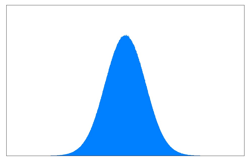
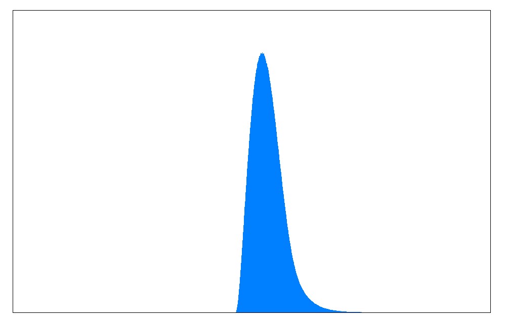
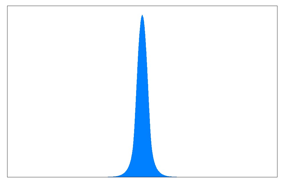
Figure 1. Distributions of normalized $L$-polynomial coefficients $a_{1},a_{2},a_{3}$ for $y^{2}=x^{7}-x+1$ over primes $p\leq 2^{30}$.

We also used our algorithm to compute Sato–Tate statistics for several other hyperelliptic curves of genus 3, including the curve

$$y^{2}=x^{7}+3x^{6}+2x^{5}+6x^{4}+4x^{3}+12x^{2}+8x,$$

which has an unusual Sato–Tate distribution as can be seen in Figure 2. This curve was found in a large search of genus 3 hyperelliptic curves with small coefficients. This curve has a non-hyperelliptic involution $[x:y:z]\mapsto[z:y/4:x/2]$, which implies that its Jacobian has extra endomorphisms and its Sato–Tate group must be a proper subgroup of $\mathrm{USp}(6)$ (the exact group has yet to be determined).

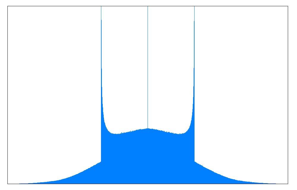
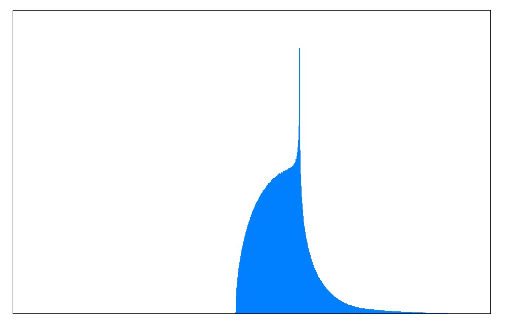
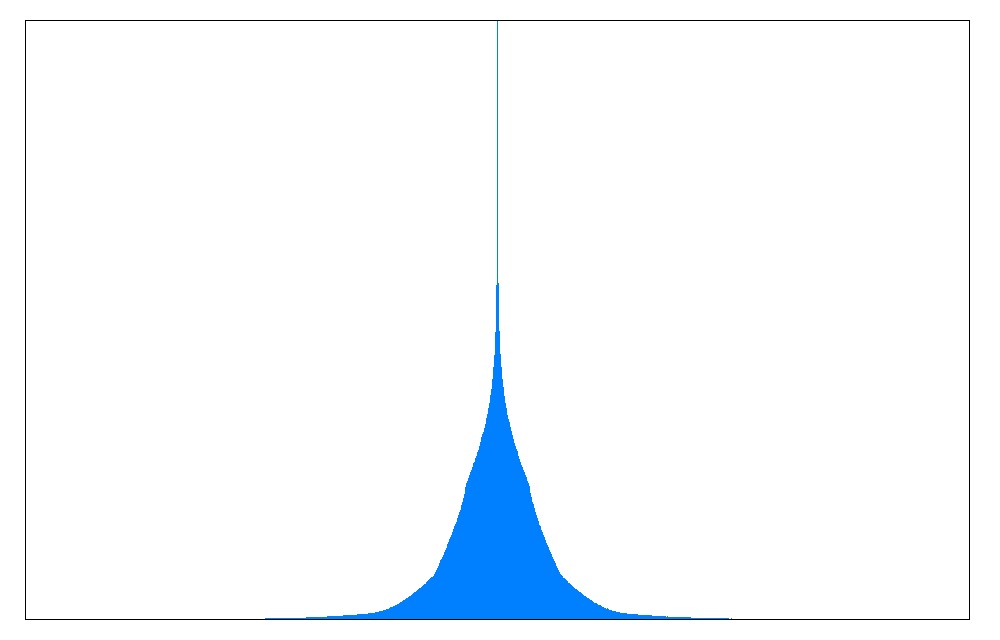
Figure 2. Distributions of normalized $L$-polynomial coefficients $a_{1},a_{2},a_{3}$ for $y^{2}=x^{7}+3x^{6}+2x^{5}+6x^{4}+4x^{3}+12x^{2}+8x$ over good primes $p\leq 2^{30}$.

More examples can be found at http://math.mit.edu/~drew.

References

• [1] Alin Bostan, Pierrick Gaudry, and Éric Schost, Linear recurrences with polynomial coefficients and application to integer factorization and Cartier-Manin operator, SIAM J. Comput. 36 (2007), no. 6, 1777–1806. MR 2299425 (2008a:11156)
• [2] A. Eisinberg and G. Fedele, On the inversion of the Vandermonde matrix, Appl. Math. Comput. 174 (2006), no. 2, 1384–1397. MR 2220623
• [3] Francesc Fité, Kiran S. Kedlaya, Víctor Rotger, and Andrew V. Sutherland, Sato-Tate distributions and Galois endomorphism modules in genus $2$, Compos. Math. 148 (2012), no. 5, 1390–1442. MR 2982436
• [4] M. Fürer, Faster integer multiplication, SIAM J. Comput. 39 (2009), no. 3, 979–1005.
• [5] David Harvey, hypellfrob software library, version 2.1.1 available at http://web.maths.unsw.edu.au/~davidharvey/code/hypellfrob/hypellfrob-2.1.1.tar.gz, 2008.
• [6] by same author, Kedlaya’s algorithm in larger characteristic, Int. Math. Res. Not. IMRN (2007), no. 22, Art. ID rnm095, 29. MR 2376210 (2009d:11096)
• [7] by same author, Computing zeta functions of arithmetic schemes, preprint http://arxiv.org/pdf/1402.3439.pdf, 2014.
• [8] by same author, Counting points on hyperelliptic curves in average polynomial time, Ann. of Math. (2) 179 (2014), no. 2, 783–803.
• [9] David Harvey, Grégoire Lecerf, and Joris van der Hoeven, Even faster integer multiplication, preprint http://arxiv.org/abs/1407.3360, 2014.
• [10] David Harvey and Andrew V. Sutherland, Computing Hasse–Witt matrices of hyperelliptic curves in average polynomial time, Algorithmic Number Theory Eleventh International Symposium (ANTS XI), vol. 17, London Mathematical Society Journal of Computation and Mathematics, 2014, pp. 257–273.
• [11] David Harvey and Joris van der Hoeven, On the complexity of integer matrix multiplication, preprint http://hal.archives-ouvertes.fr/hal-01071191, 2014.
• [12] Kiran S. Kedlaya, Counting points on hyperelliptic curves using Monsky-Washnitzer cohomology, J. Ramanujan Math. Soc. 16 (2001), no. 4, 323–338. MR 1877805 (2002m:14019)
• [13] Kiran S. Kedlaya and Andrew V. Sutherland, Computing $L$-series of hyperelliptic curves, Algorithmic Number Theory Eighth International Symposium (ANTS VIII), Lecture Notes in Comput. Sci., vol. 5011, Springer, Berlin, 2008, pp. 312–326. MR 2467855 (2010d:11070)
• [14] Ju. I. Manin, The Hasse-Witt matrix of an algebraic curve, AMS Translations, Series 2 45 (1965), 245–264, (originally published in Izv. Akad. Nauk SSSR Ser. Mat. 25 (1961) 153–172). MR 0124324 (23 #A1638)
• [15] L. J. Mordell, The congruence $(p-1/2)!\equiv\pm 1$ $({\rm mod}$ $p)$, Amer. Math. Monthly 68 (1961), 145–146. MR 0123512 (23 #A837)
• [16] J. Pila, Frobenius maps of abelian varieties and finding roots of unity in finite fields, Math. Comp. 55 (1990), no. 192, 745–763. MR 1035941 (91a:11071)
• [17] A. Schönhage and V. Strassen, Schnelle Multiplikation grosser Zahlen, Computing (Arch. Elektron. Rechnen) 7 (1971), 281–292. MR 0292344 (45 #1431)
• [18] René Schoof, Elliptic curves over finite fields and the computation of square roots mod $p$, Math. Comp. 44 (1985), no. 170, 483–494. MR 777280 (86e:11122)
• [19] Jean-Pierre Serre, Lectures on $N_{X}(p)$, Chapman & Hall/CRC Research Notes in Mathematics, vol. 11, CRC Press, Boca Raton, FL, 2012. MR 2920749
• [20] Henning Stichtenoth, Algebraic function fields and codes, Universitext, Springer-Verlag, Berlin, 1993. MR 1251961 (94k:14016)
• [21] Andrew V. Sutherland, smalljac software library, version 4.0.23 available at http://math.mit.edu/~drew/smalljac_v4.0.23.tar, 2013.
• [22] Joachim von zur Gathen and Jürgen Gerhard, Modern computer algebra, third ed., Cambridge University Press, Cambridge, 2013. MR 3087522
• [23] Noriko Yui, On the Jacobian varieties of hyperelliptic curves over fields of characteristic $p>2$, J. Algebra 52 (1978), no. 2, 378–410. MR 0491717 (58 #10920)
• [24] Yuri G. Zarhin, Hyperelliptic Jacobians without complex multiplication, Math. Res. Lett. 7 (2000), no. 1, 123–132. MR 1748293 (2001a:11097)