Finding Near-optimal Solutions in Multi-robot Path Planning

Abstract

We deal with the problem of planning collision-free trajectories for robots operating in a shared space. Given the start and destination position for each of the robots, the task is to find trajectories for all robots that reach their destinations with minimum total cost such that the robots will not collide when following the found trajectories. Our approach starts from individually optimal trajectory for each robot, which are then penalized for being in collision with other robots. The penalty is gradually increased and the individual trajectories are iteratively replanned to account for the increased penalty until a collision-free solution is found. Using extensive experimental evaluation, we find that such a penalty method constructs trajectories with near-optimal cost on the instances where the optimum is known and otherwise with 4-10 % lower cost than the trajectories generated by prioritized planning and up to 40 % cheaper than trajectories generated by local collision avoidance techniques, such as ORCA.

I Introduction

Thanks to recent advances in robotics, teams of autonomous robotic systems start to pervade not only industrial settings, but also our private spaces. Apart from numerous deployments in military settings [12], autonomously navigating robots are more and more found in warehouses and manufacturing plants [18], many private households make use of autonomous cleaning robots, and transport systems consisting of large numbers of unmanned areal vehicles (UAVs) are considered for delivering medium sized packages to the consumers.

One of the important problems in multi-robotics is simultaneous operation of multiple autonomous vehicles in shared spaces and their mutual collision avoidance. That is, given a number of vehicles, together with their starting and destination positions, we are interested in finding a set of individual trajectories so that the do not collide with each other, while at the same time the overall costs (e.g., sum of trajectory lengths) is minimized.

The problem of finding such trajectories has been studied under different names since at least 1980s. It is known that even the simple variant of the problem involving rectangular-shaped vehicles in a bounded 2-d space is PSPACE-hard [7]. While the problem is relatively straightforward to formulate as a planning problem in the Cartesian product of the state spaces of the individual robots, the solutions are difficult to find using standard search techniques because the joint state-space grows exponentially with the number of robots. The complexity can be partly mitigated using independence detection techniques such as ID [13] and M* [17] which detect independent conflict clusters and solve the resulting lower-dimensional problems separately. However, each such sub-conflict can be still prohibitively large to solve.

Prioritized planning [5, 3] is a heuristic approach based on the idea of sequential planning for the individual robots in the order of their priorities, where each robot considers the trajectories of higher-priority robots as moving obstacles and plans its trajectory to avoid them. While fast, prioritized planning is incomplete and often fails to find a solution even if one exists. Moreover, due to its greedy nature, the resulting trajectories are typically noticeably suboptimal.

Reactive approaches based on the velocity obstacle paradigm such as DRCA [9] or ORCA [15] are also popular in practice thanks to their computational efficiency. However, they resolve conflicts only locally and thus they cannot guarantee that the resulting motion will be deadlock-free.

Efficient guaranteed algorithms such as Push&Rotate [4] and Bibox [14] exist for a specific formulation of the problem, where the robots move on a graph, and each robot occupies exactly one vertex. A collision occurs only if two robots occupy the same vertex or travel on the same edge. Hence, these techniques are not suitable for fine-grained planning of robot’s motion, where the collision is defined in terms of the separation distance between the robots.

The techniques of mathematical optimization have been also studied in the context trajectory generation. In particular, the penalty-based approaches [10] have been tried for single-robot trajectory generation [11] and for the rendezvous multi-robot planning problem [2].

We explore the penalty-based approach in the context of multi-robot path finding for collision avoidance and introduce the k-step penalty method that can be seen as a generalization of prioritized planning approach. The approach solves the multi-robot path planning problem by performing a series of single-robot path planning queries in a dynamic environment in which trajectories that get close to trajectories of other robots are penalized. That is, starting from trajectories that disregard collisions with other robots, the conflicts between robots’ trajectories are gradually being penalized with increasing severity so as to finally, in a limit, the trajectories of individual robots are forced out of conflict regions as the penalties tend to infinity. Using extensive experiments, we demonstrate that this heuristic approach tends to generate near-optimal trajectories that are of significantly lower cost than the trajectories generated by currently used techniques for collision avoidance prioritized planning and ORCA [15].

After a brief problem statement in the following section, Section III introduces the kPM algorithm. Subsequently, Section IV provides an extensive experimental evaluation and analysis of the algorithm’s performance and compares it with the relevant state-of-the-art algorithms in terms of success rate, solution quality and runtime. Finally, Section V concludes the paper with a discussion of its contributions.

II Multi-robot Path Planning

Consider a team of circular mobile robots indexed $1,\ldots,n$, each with a radius $r_{i}>0$ operating in a shared 2-d workspace with static obstacles. Each robot has a task to move from its start position $s_{i}$ to some goal position $g_{i}$. A trajectory of robot $\pi_{i}$ is a mapping $\pi_{i}(t):\,\left[0,\infty\right)\rightarrow\mathbb{R}^{2}$ representing the position of the center of the robot at each future time point. A trajectory of each robot is required to start at the robot’s starting position $s_{i}$ and finish at its goal position $g_{i}$. Further, each such trajectory $\pi_{i}$ bears a cost, denoted $c(\pi_{i})$. For simplicity, we will identify the cost of a trajectory with the time the robot spends outside its destination position.

We say that two trajectories $\pi_{i},\pi_{j}$ are conflict-free iff the bodies of the two robots never intersect during the execution of their trajectories. More formally, for robots $i$ and $j$ we require that for each time-point $t\in\left[0,\infty\right)$, the distance of the corresponding robots’ positions is greater than the sum of their radii, formally:

$$\forall t\in\left[0,\infty\right):\>\left|\pi_{i}(t),\pi_{j}(t)\right|>r_{i}+r_{j},$$

where $\left|\cdot,\cdot\right|$ is the Euclidean distance between two points.

Given the assumptions above, the multi-robot path planning problem is to find a set of trajectories $\pi_{1}^{*},\ldots,\pi_{n}^{*}$ corresponding to the individual robots $1,\ldots,n$, such that i) each pair of trajectories $\pi_{i},\pi_{j}$ with $i\neq j$ is conflict-free, and ii) the sum of trajectory costs $\sum_{i=1}^{n}c(\pi_{i})$ is minimal.

To solve the problem, we could consider all robots in the system as one composite robot with many degrees of freedom and use some path planning algorithm to find a joint path for all the robots. However, the size of such a joint configuration space grows exponentially with the number of robots and thus this approach quickly becomes impractical if one wants to plan for more than a few robots.

A pragmatic approach that is often useful even for large multi-robot teams is prioritized planning. The idea has been first articulated by Erdman and Lozano-Pérez in [5]. In prioritized planning each robot is assigned a unique priority. The trajectories for individual robots are then planned sequentially from the highest priority robot to the lowest priority one. For each robot a trajectory is planned so that it avoids both the static obstacles in the environment as well as the higher-priority robots moving along the trajectories planned in the previous iterations. Works such as [16, 1] investigate heuristics for choosing a good priority sequence for the robots. Prioritized planning is more efficient than planning in the joint configuration space, but there are scenarios in which prioritized planning fails to provide a solution even if all possible priority sequences are tried (cf. Figure 1). Further, the solutions generated by prioritized planning are in most cases noticeably suboptimal, see Figure 2 for an example of such scenario.

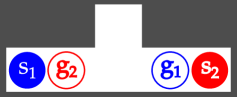
Figure 1: Corridor swap scenario: The picture shows two robots desiring to move from $s_{1}$ to $g_{1}$ ($s_{2}$ to $g_{2}$) in a corridor that is only slightly wider than a body of a single robot. Both robots move at identical maximum speeds. Irrespective of which robot starts planning first, its trajectory will be in conflict with all satisfying trajectories of the second robot.

(a) Optimal solution

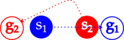
(b) Solution found by prioritized planing

Figure 2: Heads-on scenario: The picture shows two robots desiring to move from $s_{1}$ to $g_{1}$ ($s_{2}$ to $g_{2}$ resp.). The top picture illustrates how an optimal solution looks like. The bottom picture shows a solution generated by prioritized planning assuming that the robot $1$ has the higher priority: robot $1$ will follow a straight line path to its destination, without considering robot $2$, which will have to bear the full cost of avoiding the collision.

III Penalty-based Method

We propose an approach which can be seen as a generalization of prioritized planning that attempts to mitiagate the two mentioned drawbacks of the prioritized approach, but in the same time retain its tractability. We combine the idea of decoupled planning as used in prioritized planning with a process of iterative increasing of penalty, which is a popular approach for solving constrained optimization problems [10].

In the proposed approach, the requirement on minimal separation between two trajectories is modeled by a penalty function that assigns a penalty to each pair of trajectories based on how much do they violate the separation requirement. The solution to the multi-robot pathfinding problem is constructed by gradually increasing the penalty assigned when a robot passes through a collision region and by letting each robot replan its trajectory to account for the increased penalty.

Initially, the algorithm ignores interactions between the robots and finds an optimal trajectory for each robot. Then, the algorithms starts gradually increasing penalty. After each increase in weight, one of the robots is selected and a new optimal trajectory that reflects the increased penalty is found for the robot. The process is repeated until the penalties are large enough to start dominating the cost of trajectories, effectively forcing them out of the collision regions.

The minimal separation constraints between a pair of robots $i,j$ is approximated by a penalty function assigning penalty to each part of the trajectory of robot $i$ that gets closer to the trajectory of robot $j$ than the required separation distance $d_{ij}^{sep}=r_{i}+r_{j}$. The penalty function has the form

$$\Omega_{ij}(\pi_{i},\pi_{j})=\int_{0}^{\infty}\omega_{ij}(\left|\pi_{i}(t)-\pi_{j}(t)\right|)\,dt\,,$$

where $\omega_{ij}(d):\,\mathbb{R}_{\geq 0}\rightarrow\mathbb{R}_{\geq 0}$ is a continuous function assigning a time-point penalty for interaction of the trajectories $\pi_{i}$ and $\pi_{j}$ at a time-point $t$. In the case the trajectories do not violate the separation distance $d_{sep}$ at the timepoint $t$, the function assigns zero penalty. Generally, the function needs to satisfy the following conditions:

$$\forall d\enskip\begin{cases}\omega_{ij}(d)=0&\text{ if }d\geq d_{ij}^{sep}\\ \omega_{ij}(d)>0&\text{ if }d<d_{ij}^{sep}\end{cases}.$$

An example of a smooth function that satisfies these conditions is a bump function

$$\omega_{ij}(d)=\begin{cases}\frac{p_{\mathit{max}}}{e^{-s}}\cdot e^{-\frac{s}{1-(d/d_{ij}^{\mathit{sep}})^{2}})}&\textrm{for }d<d_{ij}^{\mathit{sep}}\\ 0&\mathrm{\textrm{otherwise}}\end{cases}\>,$$

where $p_{\mathit{max}}$ is a constant that can be used to adjust the penalty at $d=0$ and $s$ is a constant that can be used to adjust the “steepness” of the function. The intuition is that the “more” the vehicles violate the separation constraint in a given time-point, that is, the closer they get, the higher penalty should be assigned to the violation in that time-point. Figure 3a depicts example plots of three bump functions having different values of the parameter $s$.

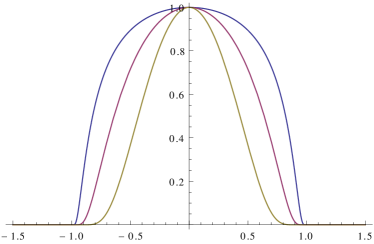
(a) Three bump functions with parameters $p_{\mathit{max}}=1$, $d_{ij}^{\mathit{sep}}=1$ and $s=1/3$ (blue), $s=1$ (purple) and $s=3$ (yellow)

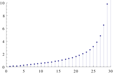
(b) Example 30 elements long weight sequence $w_{1},\ldots,w_{30}$

Figure 3: Penalty function and weight sequence function

1 Algorithm PM(k)

2      

3      for $i\leftarrow 1\ldots n$ do

4            

5            $\pi_{i}\leftarrow$Replan($i,0$);

6            

7      

8      for $i\leftarrow 1\ldots n(k-2)$ do

9            

10            $r\leftarrow i\mathrm{\>mod}\>n(k-2)$;

11            

12            $w_{i}\leftarrow\tan(\frac{i}{n(k-2)+1}\cdot\frac{\pi}{2})$;

13            

14            $\pi_{i}\leftarrow$Replan($i,w_{i}$);

15            

16      

17      for $i\leftarrow 1\ldots n$ do

18            

19            $\pi_{i}\leftarrow$Replan($i,\infty$);

20            

21      

22      if $\forall_{ij}\>\Omega_{ij}(\pi_{i},\pi_{j})=0$ then

23            

24            return $\left\langle\pi_{1},\ldots,\pi_{n}\right\rangle$;

25            

26      else

27            

28            report failure;

29            

30      

31

32Function Replan($r,w$)

33      

34      return trajectory $\pi$ for robot $r$ that minimizes $c(\pi)+\underset{j\neq r}{w\sum\,}\Omega_{rj}(\pi,\pi_{j})$ ;

35      

36

Algorithm 1 k-step Penalty Method

Algorithm 1 exposes the k-step Penalty Method (kPM) algorithm that replans the trajectory of each robot exactly $k$-times. The algorithm starts by finding a cost-optimal trajectory for each robot using $w=0$, i.e., while ignoring interactions with other robots. Then, it gradually increases the weight $w$ and thus the penalties start to be taken into account. After each increase of the weight coefficient, one of the robots is selected and its trajectory is replanned to account for the increased penalty. After the iterative phase finishes, the trajectories of all robots are replanned for the last time with the weight coefficient set to infinity. If the final set of trajectories is conflict-free, the algorithm returns the trajectories as a valid solution, otherwise it reports failure.

Since each robot replans once in the beginning (line 1) and once at the end (line 1) of the algorithm, the robot is left with $k-2$ opportunities for replanning in the iterative phase of the algorithm. Hence, it performs $n(k-2)$ iterations in the iterative stage with all the robots taking turns in a round-robin fashion (line 1).

During the iterative phase, the weights are increased in a sequence $w_{1},\ldots,w_{l}$, with $l=n(k-2)$. To model the gradual hardening of the separation constraints ultimately to the hard separation constraint, the sequence needs to converge to infinity. One way of generating such a sequence is using functions of the following form $w_{i}=\tan(\frac{i}{l+1}\cdot\frac{\pi}{2})$ for $i=1,\ldots,l$. Figure 3b shows an example plot of such a sequence.

In each iteration of the algorithm, a selected robot can generally respond in two ways to a weight increase. On the one hand side, it can accept the increase and simply leave its trajectory unchanged. On the other hand side, in can find a higher-cost trajectory that avoids the penalized region. The optimal trajectory for the robot, however, often lies in between these two extremes and avoids the penalty region only partially such that the increased cost of the trajectory with decreased received penalty are optimally traded off. This corresponds to finding a optimal trajectory subject to a spatio-temporal cost function. To find such a trajectory we discretize the free space in form of a grid-like graph and add a discretized time dimension. An optimal discrete solution is then obtained by running the A* algorithm on such a space-time graph.

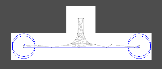
(a) The graph used for trajectory planning (in gray).

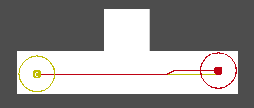
(b) Initial trajectories

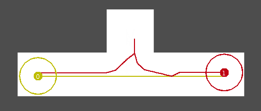
(c) Trajectories at iteration 3

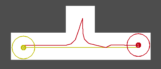
(d) Trajectories at iteration 9. Final.

Figure 4: Corridor swap scenario: two robot have to swap their positions in the depicted narrow corridor. The frames show intermediate solutions generated by PM(k=10). A video showing the resolution process and simulated execution of the solution can be watched at http://youtu.be/HartJqN5HXM.

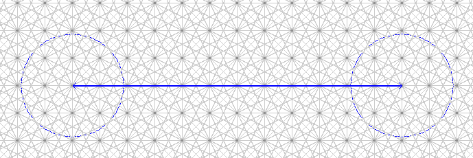
(a) The graph used for trajectory planning (in gray).

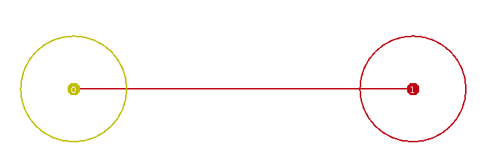
(b) Initial trajectories.

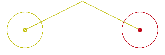
(c) Trajectories at iteration 19.

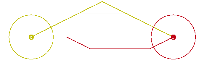
(d) Trajectories at iteration 20.

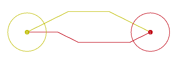
(e) Trajectories at iteration 21.

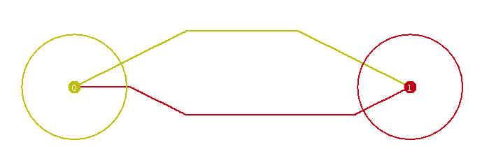
(f) Trajectories at iteration 23.

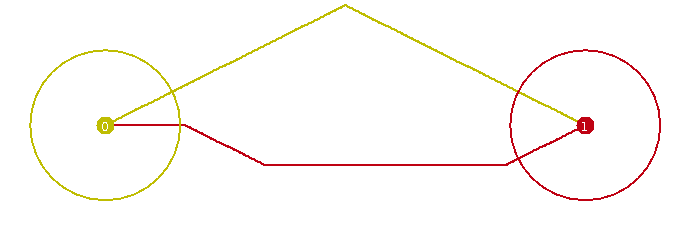
(g) Trajectories at iteration 30. Final. (Cost: 21.84)

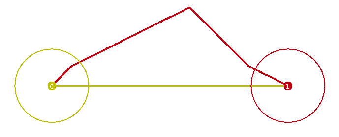
(h) Solution found by prioritized planning. (Cost: 22.68)

Figure 5: Heads-on scenario: the two robots need to swap their position in empty space. The frames show intermediate solutions generated by PM(k=20). A video showing the resolution process and simulated execution of the solution can be watched at http://youtu.be/E7LFPIi3zhQ.

Illustration of benefits

The penalty method has two benefits over prioritized planning. First, the penalty method can solve instances that are out of reach of prioritized planning. For example, the corridor swap scenario (introduced in Figure 1) can be resolved by the penalty method in $k=10$ iterations. Figure 4 illustrates how penalty method resolves the corridor swap problem. Second, for many problem instances, the penalty method can find cheaper solutions than prioritized planning. For instance, if the penalty method is applied to the heads-on scenario (introduced in Figure 2), the algorithm constructs a solution in which both robots slightly divert theirs trajectories and divide the cost of collision avoidance. This solution is cheaper then the solution returned by prioritized planning in which one of the robots takes all the cost. Figure 5 illustrates how penalty method resolves the heads-on problem.

IV Experimental Evaluation

In this section we compare the performance of our k-step penalty method (abbreviated as PM or PM(k=$\ldots$)) against prioritized planning (PP) and a state-of-the-art optimal algorithm called operator decomposition (OD) on a range of dense multi-robot path planning instances. Specifically, we focus on small and dense collision situations in which all robots are involved in a single conflict cluster. These situations usually represent bottlenecks in solving multi-robot pathfinding problems since sparser scenarios can be in most cases decomposed into a number of independent conflict clusters and solved separately.

Since reactive techniques based on the velocity obstacle paradigm [6] are often used as a practical approach for collision avoidance between robots in multi-robot teams, we also compare our method with optimal reciprocal collision avoidance (ORCA), one of the most popular algorithms belonging to this family.

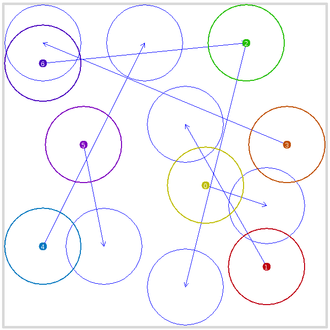
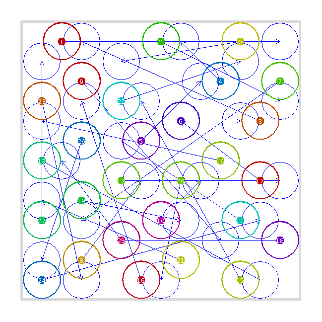
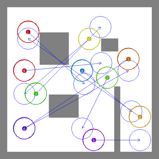
example instance, 7 robots	example instance, 25 robots	example instance, 10 robots
(a) Scenario A	(b) Scenario B	(c) Scenario C

Figure 6: Experimental environments

Experiment setup

The experimental comparison is done in three environments depicted in Figure 6. The robots are modeled as 2-d discs that move on a 16-connected grid graph depicted in Figure 7. The start and goal position for each robot is chosen randomly. When generating start and destination for each robot we ensure that a) robots do not overlap at start position, b) robots do not overlap at goal position, and c) when adding a robot, its individually optimal trajectory must be in conflict with the trajectory of some previously added robot, i.e. the robots form a single conflict cluster. In Scenario A and B, the start and destination for each robot is chosen from the area depicted by the gray rectangle, however, the robots are allowed to leave the rectangle when resolving the conflict. In Scenario C, the robots cannot leave the free space when resolving the conflict. All robots can move at the same maximum speed.

We generated 25 random problem instances for different numbers of robots in each environment. On each instance we run all the algorithms and record the solution quality of the returned solution and the runtime. The bars in the graphs indicate standard error of the average. Experiment runs were executed on 1 core of Intel Xeon E5-2665 2.40GHz, 4 GB RAM. A bundle that includes implementation of all the algorithms together with the problem instances can be downloaded at http://agents.fel.cvut.cz/~cap/kpm.

Algorithms used in the comparison

Penalty Method (PM)

The penalty-based method described in Section III was tried for different values of parameters $k$ ranging from $k=3$ to $k=100$.

Prioritized Planning (PP)

In prioritized planning (PP) we use a fixed random priority ordering over the robots. The ordering used in PP identical to the ordering used in the penalty method.

Operator Decomposition (OD)

Operator Decomposition [13] is a complete and optimal forward-search algorithm for multi-robot path planning on a graph representing a discretization of the joint state space of a number of robots. The joint state space is searched using the operator decomposition technique that decomposes joint-actions to trees of single-robot moves, which allows more efficient pruning and better utilization of a heuristic estimate during the search process. We use OD algorithm to find provably optimal solutions.

Optimal Reciprocal Collision Avoidance (ORCA)

The reactive technique ORCA [15] is typically used as a closed-loop controller that at each time instant selects collision-avoiding velocity vector from the continuous space of robot’s velocities that is the closest to the robot’s desired velocity. In our implementation, at each time instant the algorithm computes a shortest path from the robots current position to its goal on the same graph that is used by other methods. The desired velocity vector then points at the this shortest path at the maximum speed. When using ORCA, we often witnessed dead-lock situations during which the robots either moved at extremely slow velocity or stopped completely. If a prolonged deadlock situation was detected, we considered the run as failed.

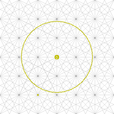
(a) Discretization used in Scenario A

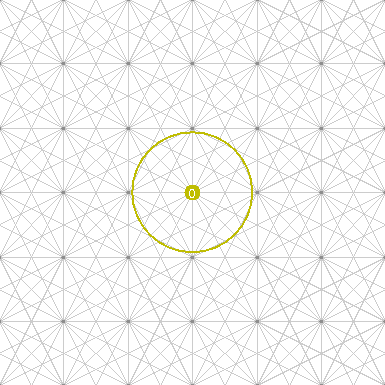
(b) Discretization used in Scenario B and C

Figure 7: Discretization used for trajectory planning

Results

Success rate

The comparison of success rate of the tested algorithms is in Figure  8. The plots shows the ratio of successfully solved instances for each algorithm in each test environment. Since the runtime of OD grows exponentially, we limited the runtime of OD to 1 hour. The simulation of ORCA was terminated with failure if a deadlock was detected.

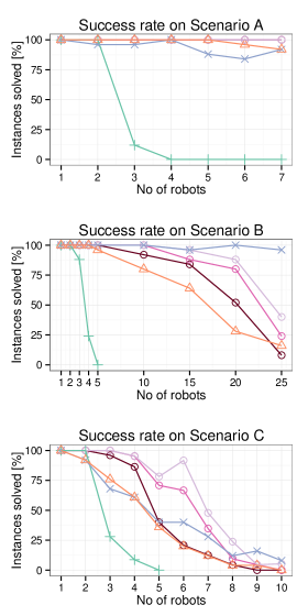
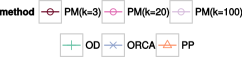
Figure 8: Success rate. The plot shows the percentage of instances successfully solved by PM, PP, ORCA and OD in each environment. From PM, three different values of $k$ parameter are considered: $k=3$, $k=20$, and $k=100$.

Sub-optimality

Figure 9 shows average sub-optimality of solutions returned by the PM algorithm for different values of $k$ parameter in each environment. The average suboptimality of solutions returned by PP algorithm is also shown for each environment. The sub-optimality of a solution on a particular instance is computed as $-(c-c^{*})/c^{*}$, where $c$ is the cost of the solution returned by the measured algorithm and $c^{*}$is the cost of optimal solution computed using OD algorithm. The averages are computed only from the subset of instances that were successfully resolved by all tested algorithms and for which we were able to compute the optimum.

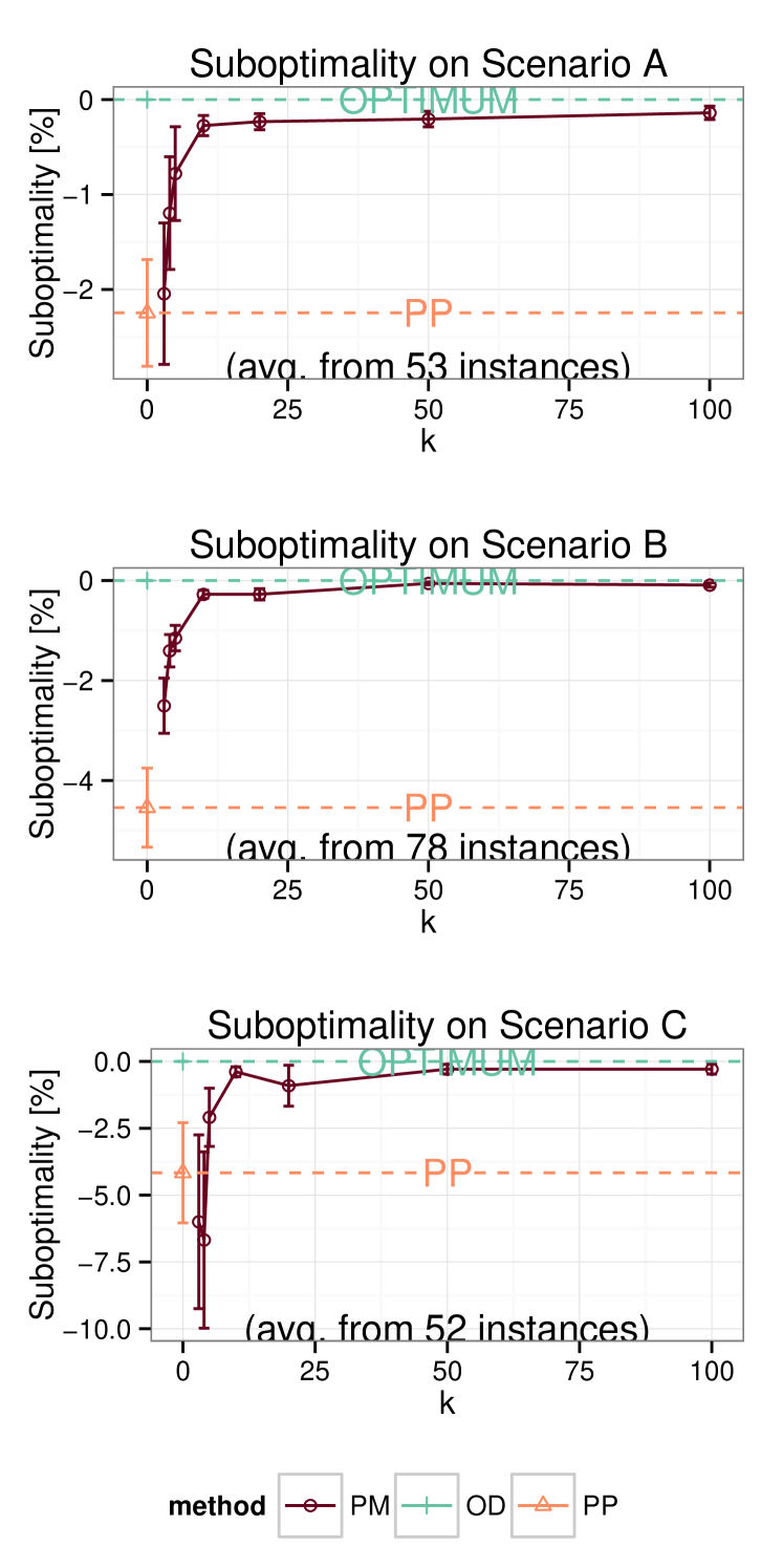
Figure 9: Optimality of penalty method. The plot shows average suboptimality of solutions returned by PM for different values of $k$ parameter ranging from $k=3$ to $k=100$. The averages are computed on instances for which we were able to compute the optimum using the OD algorithm.

Time spent outside goal

Figure 10 shows the average time spent outside goal position when the robots execute the solutions found by PM, PP and ORCA in all instances in Scenario B that involve 10 robots. The averages are computed on the subset of instances that were successfully resolved by all compared algorithms.

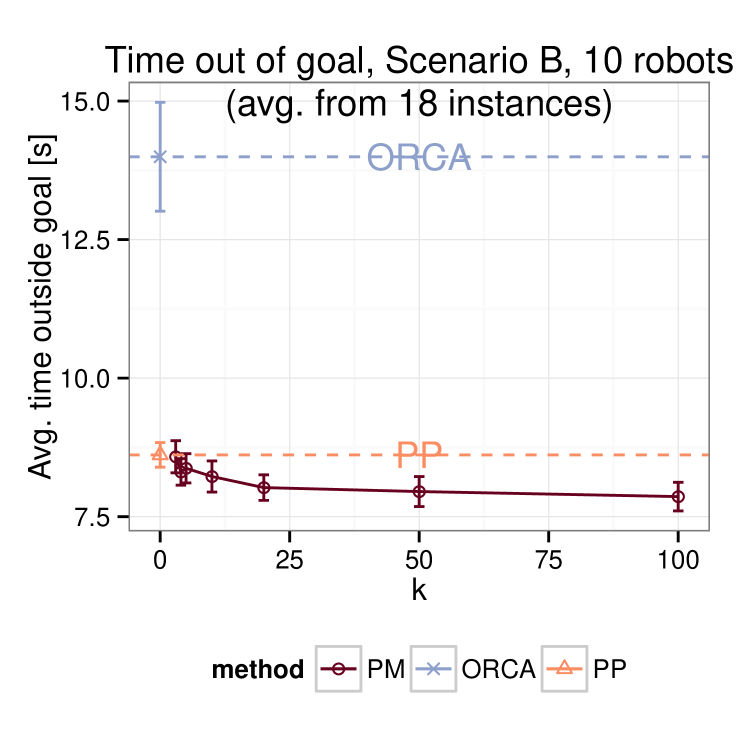
Figure 10: Average time spent outside goal (i.e. cost). The plot shows average time the robots spend outside the goal if they execute solutions found by PM, PP and ORCA. For PM, we consider values of $k$ ranging from $k=3$ to$k=100$. Measured on all instances with 10 robots in Scenario B that were successfully solved by all compared methods.

CPU runtime

Figure 11 shows average CPU runtime that PM and PP algorithms require to return a solution. The averages are computed only on the subset of instances that were successfully resolved by both PP and PM.

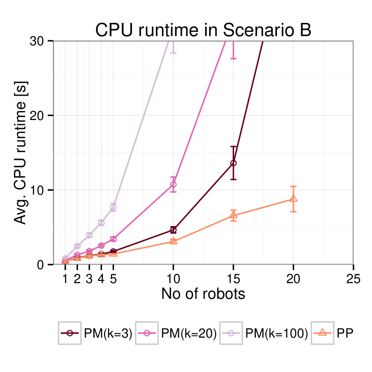
Figure 11: CPU runtime requirements. The plot shows average CPU runtime needed by PM and PP to return solution in instances involving different numbers of robots. From PM, three different values of $k$ parameter are considered: $k=3$, $k=20$, and $k=100$.

Results interpretation

Our results show that the optimal algorithm OD is practical only for instances that contain three or fewer robots. Prioritized planning generally scales better than OD, but returns solutions that are on average 2-4 % suboptimal (cf. Figure 9). Although PM requires more time to provide a solution than PP (cf. Figure 11), it does not exhibit the exponential drop in ability to solve larger instances that OD suffers from. Yet, the cost of solutions returned by PM tend to converge to the vicinity of the optimal cost with increasing number of iterations $k$ for the instances where the optimum is known, (cf. Figure 9) and otherwise converges to solutions that are of significantly lower cost than the solutions returned by PP (cf. Figure 10). Further, besides the improved quality of the returned solutions, PM achieves higher success-rate on our instances (cf. Figure 8). E.g., in the empty environment with 20 robots (cf. Figure 8), PM(k=100) solves 88 % of the instances, where PP solves only 28 %.

Although ORCA exhibits high success rate on our instances in Scenario B, it should be noted that the trajectories resulting from this collision avoidance process are very costly. We have observed that in instances involving higher number of robots kPM returns trajectories that are more than 40 % faster than the trajectories returned by ORCA (cf. Figure 10).

Real-world maps

To demonstrate the applicability of our method, we have deployed the penalty method to coordinate trajectories of a number of simulated robots in two representative real-world environments. First, we tested the algorithm in an office corridor environment, which is based on the laser rangefinder log of Cartesium building at the University of Bremen. The environment and the roadmap used for trajectory planning in the environment together with the task of each robot are depicted in Figure 12a. We run PM(k=5) algorithm to coordinate the trajectories of 16 robots sharing the environment and after 19 seconds obtained the trajectories shown in Figure 12b. A video showing simulated execution of the found trajectories can be watched at http://youtu.be/VfiBuQBBIhM.

Second, we depolyed the algorithm in a logistic center environment. The tasks of the individual robots and the roadmap that the robots used for planning in this environment are shown in Figure 13a. We used PM(k=5) algorithm to coordinate the trajectories of the individual robots. After 55 seconds we obtained coordinated trajectories shown in Figure 13b. The simulated execution of the found trajectories can be watched at http://youtu.be/G3A3TYKu73Q.

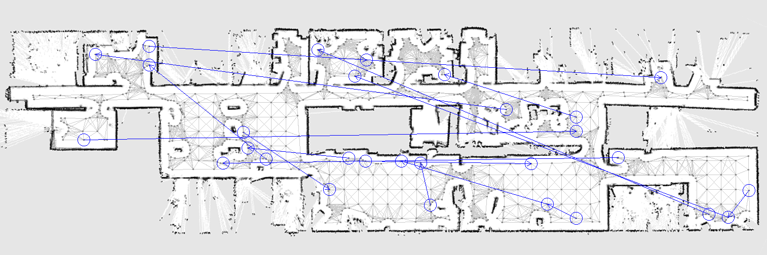
(a) Tasks of the robots and the roadmap used for planning.

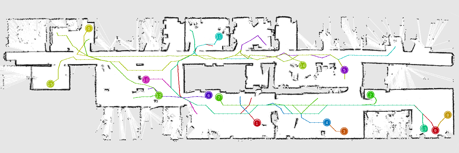
(b) Resulting coordinated trajectories.

Figure 12: Office corridor: Coordination of 16 robots in an office corridor.

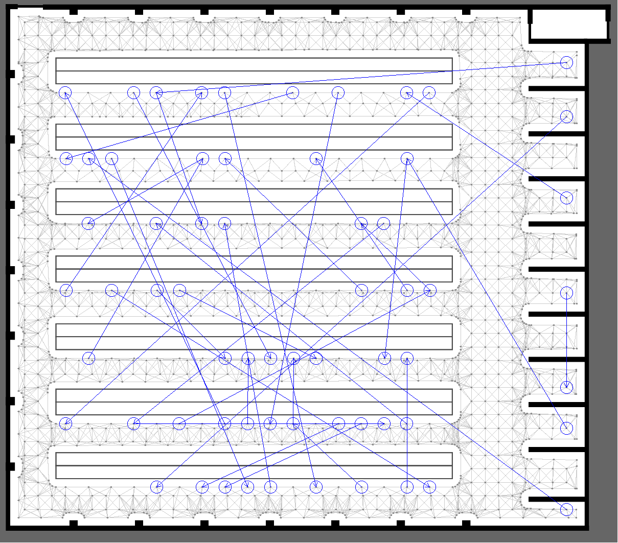
(a) Tasks of the robots and the roadmap used for planning.

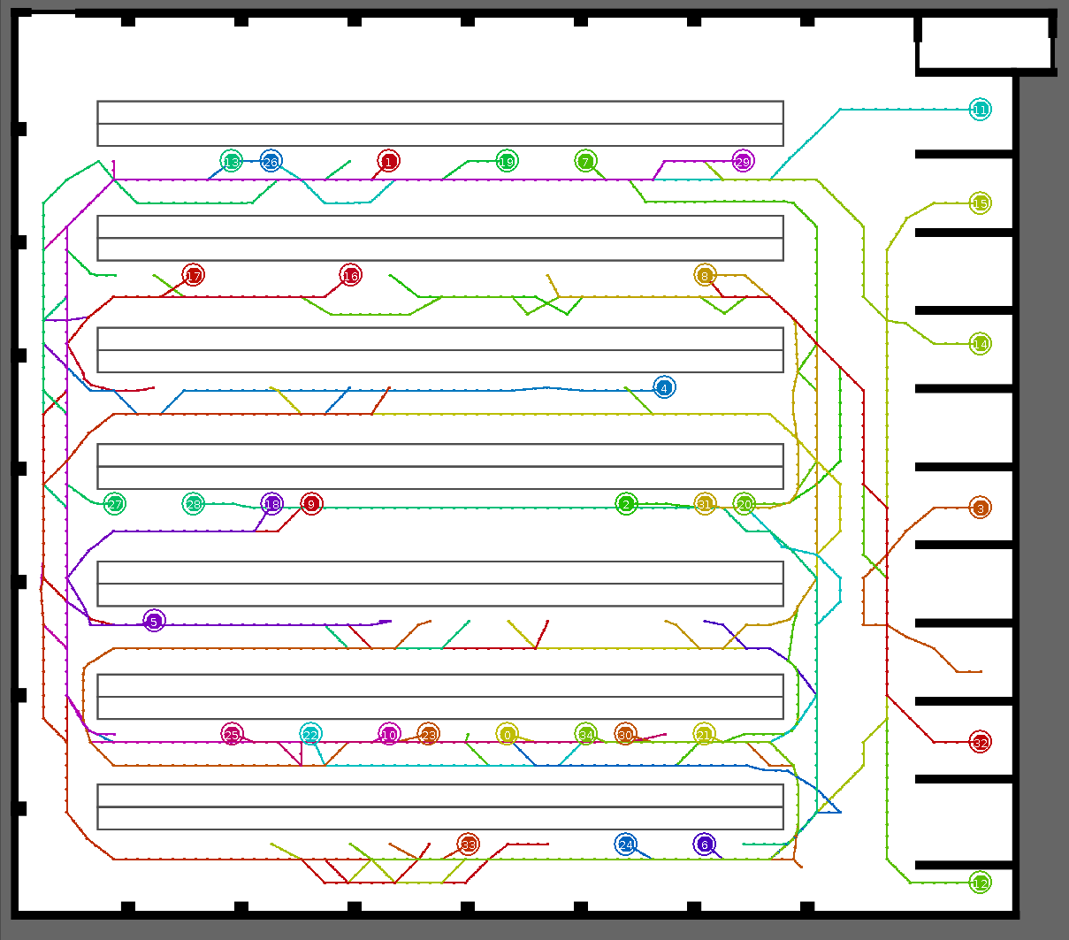
(b) Resulting coordinated trajectories.

Figure 13: Logistic center: Coordination of 35 robots in a logistic centers.

V Conclusion

In this work we have explored the applicability of penalty-based method to improve success rate and the quality of returned solution of prioritized planning. We have formulated a new penalty-based algorithm for finding collision-avoiding trajectories in multi-robot teams. The algorithm starts from an individually optimal trajectory for each robot. Then, the parts of the trajectories that lie in collision with other robots are penalized and the magnitude of the penalty is gradually increased towards infinity. After each such increase, the trajectory of one of the robots is replanned to account for the increased penalty. Using this process, the trajectories are gradually forced out of collisions.

We have compared our penalty-based method with a state-of-the-art optimal algorithm, prioritized planning and reactive technique ORCA on three benchmark scenarios. Our results show that with increasing number of iterations, the algorithm constructs solutions with near-optimal cost (on instances where the optimum was known). On the instances where the optimum was not known, our method consistently provided solutions that are 4-10 % cheaper than solutions provided by prioritized planning and up to 40 % cheaper than the solutions provided by a widely-used reactive technique ORCA.

References

- [1] M. Bennewitz, W. Burgard, and S. Thrun. Finding and optimizing solvable priority schemes for decoupled path planning techniques for teams of mobile robots. Robotics and Autonomous Systems, 41(2):89–99, 2002.
- [2] Subhrajit Bhattacharya, Vijay Kumar, and Maxim Likhachev. Distributed optimization with pairwise constraints and its application to multi-robot path planning. In Robotics: Science and Systems, 2010.
- [3] Michal Cap, Peter Novak, Jiri Vokrinek, and Michal Pechoucek. Asynchronous decentralized algorithm for space-time cooperative pathfinding. In Spatio-Temporal Dynamics Workshop (STeDy), SFB/TR 8 Spatial Cognition Center Report, No. 030-08/2012, 2012.
- [4] Boris de Wilde, Adriaan W ter Mors, and Cees Witteveen. Push and rotate: cooperative multi-agent path planning. In Proceedings of the 2013 international conference on Autonomous agents and multi-agent systems, pages 87–94. International Foundation for Autonomous Agents and Multiagent Systems, 2013.
- [5] Michael Erdmann and Tomas Lozano-Pérez. On multiple moving objects. Algorithmica, 2:1419–1424, 1987.
- [6] Paolo Fiorini and Zvi Shiller. Motion planning in dynamic environments using velocity obstacles. The International Journal of Robotics Research, 17(7):760–772, 1998.
- [7] J.E. Hopcroft, J.T. Schwartz, and M. Sharir. On the complexity of motion planning for multiple independent objects; pspace- hardness of the "warehouseman’s problem". The International Journal of Robotics Research, 3(4):76–88, December 1984.
- [8] Andrew Howard and Nicholas Roy. The robotics data set repository (radish), 2003.
- [9] E. Lalish. Distributed Reactive Collision Avoidance. BiblioBazaar, 2011.
- [10] Jorge Nocedal and Stephen J. Wright. Numerical optimization. Springer series in operations research and financial engineering. Springer, New York, NY, 2. ed. edition, 2006.
- [11] John Schulman, Jonathan Ho, Alex Lee, Ibrahim Awwal, Henry Bradlow, and Pieter Abbeel. Finding locally optimal, collision-free trajectories with sequential convex optimization. In Proceedings of Robotics: Science and Systems, Berlin, Germany, June 2013.
- [12] Martin Selecký, Antonín Komenda, Michal Štolba, Tomáš Meiser, Michal Čáp, Milan Rollo, Jiří Vokřínek, and Michal Pěchouček. Deployment of multi-agent algorithms for tactical operations on uav hardware (demonstration). In Proceedings of AAMAS 2013 (to appear), 2013.
- [13] Trevor Scott Standley. Finding optimal solutions to cooperative pathfinding problems. In Maria Fox and David Poole, editors, AAAI. AAAI Press, 2010.
- [14] Pavel Surynek. A novel approach to path planning for multiple robots in bi-connected graphs. In Proceedings of the 2009 IEEE international conference on Robotics and Automation, ICRA’09, pages 928–934, Piscataway, NJ, USA, 2009. IEEE Press.
- [15] Jur Van Den Berg, Stephen Guy, Ming Lin, and Dinesh Manocha. Reciprocal n-body collision avoidance. Robotics Research, pages 3–19, 2011.
- [16] Jur van den Berg and Mark Overmars. Prioritized motion planning for multiple robots. In IROS, pages 430–435, 2005.
- [17] Glenn Wagner and Howie Choset. M*: A complete multirobot path planning algorithm with performance bounds. In IROS, pages 3260–3267, 2011.
- [18] Peter R. Wurman, Raffaello D’Andrea, and Mick Mountz. Coordinating hundreds of cooperative, autonomous vehicles in warehouses. In Proceedings of the 19th National Conference on Innovative Applications of Artificial Intelligence - Volume 2, IAAI’07, pages 1752–1759. AAAI Press, 2007.