A classical and a relativistic law of motion for spherical supernovae

Abstract

In this paper we derive some first order differential equations which model the classical and the relativistic thin layer approximations. The circumstellar medium is assumed to follow a density profile of Plummer type, or of Lane–Emden ($n=5$) type, or a power law. The first order differential equations are solved analytically, or numerically, or by a series expansion, or by recursion. The initial conditions are chosen in order to model the temporal evolution of SN 1993J over ten years and a smaller chi-squared is obtained for the Plummer case with eta=6. The stellar mass ejected by the SN progenitor prior to the explosion, expressed in solar mass, is identified with the total mass associated with the selected density profile and varies from $0.217$ to $0.402$ when the central number density is $10^{7}$ particles per cubic centimeter. The Full width at half maximum of the three density profiles, which can be identified with the size of the Pre-SN 1993J envelope, varies from 0.0071 pc to 0.0092 pc.

1 Introduction

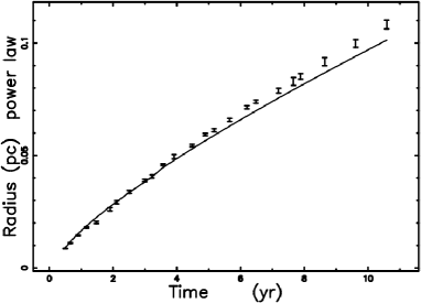
Figure 9: Theoretical radius for the power law case as obtained by the solution of the nonlinear equation connected with (30) (full line). Data as in Table 1. The astronomical data of SN 1993J are represented with vertical error bars.

The absorption features of supernovae (SN) allow the determination of their expansion velocity, $v$. We select, among others, some results. The spectropolarimetry (CA II IR triplet) of SN 2001el gives a maximum velocity of $\approx 26000\rm\,{kms^{-1}}$, see Wang et al. (2003). The same triplet when searched in seven SN of type Ia gives $10400\rm\,{kms^{-1}}\leq v\leq 17700\rm\,{kms^{-1}}$, see Table I in Mazzali et al. (2005). A time series of eight spectra in SN  2009ig allows asserting that the velocity at the CA II line, for example, decreases in 12 days from 32000 $\rm\,{kms^{-1}}$ to 21500$\rm\,{kms^{-1}}$, see Figure 9 in Marion et al. (2013). A recent analysis of 58 type Ia SN in Si II gives $9660\rm\,{kms^{-1}}\leq v\leq 14820\rm\,{kms^{-1}}$, see Table II in Childress et al. (2014). The previous analysis allow saying that the maximum velocity sofar observed for SN is $\frac{v}{c}\approx 0.1$, where $c$ is the speed of light; this observational fact points to a relativistic equation of motion.

We now briefly review the shocks and the Kompaneyets approximation in special relativity (SR). A similar solution for strong relativistic shocks in a circumstellar medium (CSM) which varies with the radius was found by Blandford & McKee (1976). Relativistic shocks are commonly used for gamma ray bursts (GRB) in order to explain the production of non-thermal electrons, see Baring (2011). The interactions between the shock and the ambient density fluctuations can produce turbulence with a significant component of magnetic energy, see Inoue et al. (2011). Relativistic radiation-mediated shocks can produce GRB with typical parameters similar to those observed, see Nakar & Sari (2012). Trans-relativistic shocks have been used to produce high-energy neutrino and gamma-ray in SN, see Kashiyama et al. (2013). The Kompaneyets approximation is usually developed in a Newtonian framework, see Kompaneyets (1960); Olano (2009), and has been derived in SR by Shapiro (1979); Lyutikov (2012). The temporal observations of SN such as SN 1993J establish a clear relation between the instantaneous radius of expansion $r$ and the time $t$, of the type $r\propto t^{0.82}$, see Marcaide et al. (2009) and therefore allows exploring variants of the thin layer approximation. The previous observational facts excludes a SN propagation in an CSM with constant density: two solutions of this type are the Sedov solution which scales as $r\propto t^{0.4}$, see Sedov (1959); McCray (1987), and the momentum conservation in a thin layer approximation, which scales as $r\propto t^{0.25}$, see Dyson, J. E. and Williams, D. A. (1997); Padmanabhan (2001). Previous efforts to model these observations in the framework of the thin layer approximation in an CSM governed by a power law, see Zaninetti (2011), or in the framework in which the CSM has a constant density but swept mass regulated by a parameter called porosity, see Zaninetti (2012), have been successfully explored. An important feature of the various models is based on the type of CSM which surrounds the expansion. As an example in the framework of classical shocks, Chevalier (1982a) and Chevalier (1982b) analyzed self-similar solutions with an CSM of the type $r^{-s}$, which means an inverse power law dependence. In the framework of the Kompaneyets equation, see Kompaneyets (1960), for the motion of a shock wave in different plane-parallel stratified media, Olano (2009) considered four types of CSM. It is therefore interesting to take into account an self-gravitating CSM, which gives a physical basis to the considered model. The relativistic treatment has been concentrated on the determination of the Lorentz factor, $\gamma$, for the ejecta in GRB; we report some research in this regard: Granot & Kumar (2006) found $30<\gamma<50$ for a significant number of GRBs, Pe’er et al. (2007) found $\gamma=305$ for GRB 970828 and $\gamma=384$ for GRB 990510, Zou & Piran (2010) found high values for the sample of the GRBs considered $30.5\gamma<900$, Aoi et al. (2010) in the framework of a high-energy spectral cutoff originating from the creation of electron–positron pairs found $\gamma\approx$ 600 for GRB 080916C, Muccino et al. (2013) found $\gamma\approx 6.7\times 10^{2}$ for GRB 090510. The last phase of stellar evolution predicts the production of ⁵⁶Ni, see Truran et al. (1967); Bodansky et al. (1968); Matz & Share (1990); Truran et al. (2012) and therefore this type of decay has been used to model the light curve of supernovae (SN), see among others Mazzali et al. (1997); Elmhamdi et al. (2003); Stritzinger et al. (2006); Magkotsios et al. (2010); Krisciunas et al. (2011); Okita et al. (2012); Chen et al. (2013) as well the reddening measurements of the supernova remnant (SNR) Cassiopeia A, see Eriksen et al. (2009). These theoretical and observational efforts give interest to the exploration of the modification of ⁵⁶Ni decay due to time dilation.

In this paper we review the standard two-phase model for the expansion of a SN, see Section 2, and three density profiles, see Section 3. In Section 4 we derive the differential equations which model the thin layer approximation for a SN in the presence of three types of medium. Section 4 also contains a model in which the center of the explosion does not coincide with the center of the polytrope. A relativistic treatment is carried out in Section 5. The application of the developed theory to SN 1993J is split into the classical case, see Section 6, and the relativistic case, see Section 7.

2 The standard model

A SN expands at a constant velocity until the surrounding mass is of the order of the solar mass. This time, $t_{M}$, is

$$t_{M}=186.45\,{\frac{\sqrt[3]{{\it M_{\sun}}}}{\sqrt[3]{{\it n_{0}}}{\it v_{10000}}}}\quad yr\quad,$$ (1)

where $M_{\sun}$ is the number of solar masses in the volume occupied by the SN, $n_{0}$ is the number density expressed in particles $\mathrm{cm}^{-3}$, and $v_{10000}$ is the initial velocity expressed in units of 10000 km/s, see McCray (1987). A first law of motion for the $SN$ is the Sedov solution

$$R(t)=({\frac{25}{4}}\,{\frac{{\it E}\,{t}^{2}}{\pi\,\rho}})^{1/5}\quad,$$ (2)

where $E$ is the energy injected into the process and $t$ is the time, see Sedov (1959); McCray (1987). Our astrophysical units are: time, ($t_{1}$), which is expressed in years; $E_{51}$, the energy in $10^{51}$ erg; $n_{0}$, the number density expressed in particles $\mathrm{cm}^{-3}$  (density $\rho=n_{0}m$, where $m=1.4m_{\mathrm{H}}$). In these units, Eq. (2) becomes

$$R(t)\approx 0.313\,\sqrt[5]{{\frac{{\it E_{51}}\,{{\it t_{1}}}^{2}}{{\it n_{0}}}}}~{}{pc}\quad.$$ (3)

The Sedov solution scales as $t^{0.4}$. We are now ready to couple the Sedov phase with the free expansion phase

$$R(t)=\{\begin{array}[]{ll}0.0157t\,\mbox{pc}&\mbox{if $t\leq 2.5$ yr }\\ 0.0273\,\sqrt[5]{t}^{2}\,\mbox{pc}&\mbox{if $t>2.5$ yr.}\end{array}$$

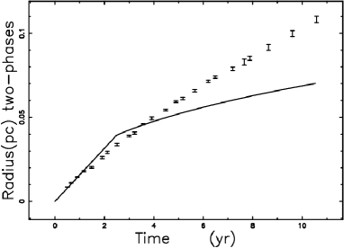
Figure 1: Theoretical radius as given by the two-phase solution (full line) and astronomical data of SN 1993J with vertical error bars.

This two-phase solution is obtained with the following parameters $M_{\sun}$ =1 , $n_{0}=1.127\times 10^{5}$, $E_{51}=0.567$ and Fig. 1 presents its temporal behavior as well as the data. A similar model is reported in Spitzer (1978) with the difference that the first phase ends at $t=60$ yr against our $t=2.5$ yr. A careful analysis of Fig. 1 reveals that the standard two-phase model does not fit the observed radius–time relation for SN 1993J .

3 Density profiles for the CSM

This section introduces three density profiles for the CSM: a Plummer-like profile, an self-gravitating profile of Lane–Emden type, and a power law profile .

3.1 The Plummer profile

The Plummer-like density profile, after Plummer (1911), is

$$\rho(r;R_{flat})=\rho_{c}({\frac{R_{flat}}{({R_{flat}^{2}+r^{2}})^{1/2}}})^{\eta}\quad$$

where $r$ is the distance from the center, $\rho$ is the density, $\rho_{c}$ is the density at the center, $R_{flat}$ is the distance before which the density is nearly constant, and $\eta$ is the power law exponent at large values of $r$, see Whitworth & Ward-Thompson (2001) for more details. The following transformation, $R_{flat}=\sqrt{3}b$, gives the Plummer-like profile, which can be compared with the Lane–Emden profile

$$\rho(r;b)=\rho_{c}\bigl{(}\frac{1}{1+\frac{1}{3}\,{\frac{{r}^{2}}{{b}^{2}}}}\bigr{)}^{\eta/2}\quad.\quad$$ (4)

At low values of $r$, the Taylor expansion of the Plummer-like profile can be taken:

$$\rho(r;b)\approx\rho_{{c}}(1-1/6\,{\frac{\eta\,{r}^{2}}{{b}^{2}}})\quad,$$

and at high values of $r$, the behavior of the Plummer-like profile is

$$\rho(r;b)\sim\rho_{c}(\sqrt{3}\,b)^{\eta}(\frac{1}{r})^{\eta}\quad.$$

The total mass $M(r;b)$ comprised between 0 and $r$ is

$$M(r;b)=\int_{0}^{r}4\pi r^{2}\rho(r;b)dr=\frac{PN}{PD}\quad,$$ (5)

where

$$PN=-\sqrt{3}b\rho_{{c}}\pi\,(4\,{\mbox{${}_{2}$F${}_{1}$}(\eta/2,-3/2+\eta/2;\,-1/2+\eta/2;\,-3\,{\frac{{b}^{2}}{{r}^{2}}})}\times$$

$$\times\Gamma(-\eta/2+5/2)\Gamma(\eta/2)\cos(1/2\,\pi\,\eta){r}^{3-\eta}{3}^{1/2+\eta/2}{b}^{\eta-1}$$

$$-9\,{\pi}^{3/2}{b}^{2}\eta+27\,{\pi}^{3/2}{b}^{2})$$

and

$$PD=3\,\cos(1/2\,\pi\,\eta)\Gamma(-\eta/2+5/2)(\eta-3)\Gamma(\eta/2)\quad,$$

where ${~{}_{2}F_{1}(a,b;\,c;\,z)}$ is the regularized hypergeometric function Abramowitz & Stegun (1965); Olver et al. (2010). The above expression simplifies when $\eta=6$ , $M(r;b)_{6}$,

$$M(r;b)_{6}={\frac{27\,\rho_{{c}}\pi\,{b}^{7}\sqrt{3}}{2\,(3\,{b}^{2}+{r}^{2})^{2}}\arctan(1/3\,{\frac{r\sqrt{3}}{b}})}+9\,{\frac{\rho_{{c}}\pi\,{b}^{5}\sqrt{3}{r}^{2}}{(3\,{b}^{2}+{r}^{2})^{2}}\arctan(1/3\,{\frac{r\sqrt{3}}{b}})}+$$

$$3/2\,{\frac{\rho_{{c}}\pi\,{b}^{3}\sqrt{3}{r}^{4}}{(3\,{b}^{2}+{r}^{2})^{2}}\arctan(1/3\,{\frac{r\sqrt{3}}{b}})}-{\frac{27\,\rho_{{c}}\pi\,{b}^{6}r}{2\,(3\,{b}^{2}+{r}^{2})^{2}}}+9/2\,{\frac{\rho_{{c}}\pi\,{b}^{4}{r}^{3}}{(3\,{b}^{2}+{r}^{2})^{2}}}\quad.$$

The astrophysical version of the total mass is

$$M(r_{pc};b_{pc})=\frac{PNA}{PDA}\,M_{\sun}\quad,$$

with

$$PNA=-2.47\,10^{-10}\,{b_{{{\it pc}}}}^{3}n_{{0}}[1.02\,10^{10}\,\arctan(1.73\,{\frac{b_{{{\it pc}}}}{r_{{{\it pc}}}}}){b_{{{\it pc}}}}^{4}$$

$$+6.8\,10^{9}\,\arctan(1.73\,{\frac{b_{{{\it pc}}}}{r_{{{\it pc}}}}}){b_{{{\it pc}}}}^{2}{r_{{{\it pc}}}}^{2}+1.13\,10^{9}\,\arctan(1.73\,{\frac{b_{{{\it pc}}}}{r_{{{\it pc}}}}}){r_{{{\it pc}}}}^{4}-1.6\,10^{10}\,{b_{{{\it pc}}}}^{4}$$

$$+5.89\,10^{9}\,{b_{{{\it pc}}}}^{3}r_{{{\it pc}}}-1.06\,10^{10}\,{b_{{{\it pc}}}}^{2}{r_{{{\it pc}}}}^{2}-1.96\,10^{9}\,b_{{{\it pc}}}{r_{{{\it pc}}}}^{3}-1.78\,10^{9}\,{r_{{{\it pc}}}}^{4}]$$

and

$$PDA=\left(3.0\,{b_{{{\it pc}}}}^{2}+{r_{{{\it pc}}}}^{2}\right)^{2}\quad,$$

where ${b_{{{\it pc}}}}$ is b expressed in pc, ${r_{{{\it pc}}}}$ is r expressed in pc and $n_{0}$ is the same of eqn.(3). The relationship between Full width at half maximum (FWHM) and ${b_{{{\it pc}}}}$ is

$$FWHM=1.766\,b_{{{\it pc}}}\quad.$$

3.2 The Lane–Emden profile

The self gravitating sphere of polytropic gas is governed by the Lane–Emden differential equation of the second order

$${\frac{d^{2}}{d{x}^{2}}}Y(x)+2\,{\frac{{\frac{d}{dx}}Y(x)}{x}}+(Y(x))^{n}=0\quad,$$

where $n$ is an integer, see Lane (1870); Emden (1907); Chandrasekhar (1967); Binney & Tremaine (2011); Zwillinger (1989).

The solution $Y(x)_{n}$ has the density profile

$$\rho=\rho_{c}Y(x)_{n}^{n}\quad,$$

where $\rho_{c}$ is the density at $x=0$. The pressure $P$ and temperature $T$ scale as

$$P=K\rho^{1+\frac{1}{n}}\quad,$$ (6)

$$T=K^{\prime}Y(x)\quad,$$ (7)

where K and K^′ are two constants, for more details, see Hansen & Kawaler (1994).

Analytical solutions exist for $n=0$, 1 and 5; that for $n$=0 is

$$Y(x)=\frac{sin(x)}{x}\quad,$$

and has therefore an oscillatory behavior. The analytical solution for $n$=5 is

$$Y(x)={\frac{1}{{(1+\frac{{x}^{2}}{3})^{1/2}}}}\quad,$$

and the density for $n$=5 is

$$\rho(x)=\rho_{c}{\frac{1}{{(1+\frac{{x}^{2}}{3})^{5/2}}}}\quad.$$ (8)

The variable $x$ is non-dimensional and we now introduce the new variable $x=r/b$

$$\rho(r;b)=\rho_{c}{\frac{1}{{(1+\frac{{r}^{2}}{3b^{2}})^{5/2}}}}\quad.$$

This profile is a particular case, $\eta=5$, of the Plummer-like profile as given by Eq. (4). At low values of $r$, the Taylor expansion of this profile is

$$\rho(r;b)\approx\rho_{{c}}(1-5/6\,{\frac{{r}^{2}}{{b}^{2}}})\quad,$$

and at high values of $r$, its behavior is

$$\rho(r;b)\sim 9\,{\frac{\rho_{{c}}\sqrt{3}{b}^{5}}{{r}^{5}}}\quad.$$ (9)

The FWHM is

$$FWHM=1.95\,b_{{{\it pc}}}\quad.$$

The gradient here is assumed to be local: it covers lengths smaller than 1 pc, and is not connected with the gradient which regulates the equilibrium of a galaxy that extends over a region of some kpc. The interaction of the progenitor star with the CSM, through stellar winds, creates a CSM. The dynamics of this medium can be far equilibrium. The main astrophysical assumption adopted here is that the density of the CSM decreases smoothly at low values of distance, as $\rho\approx A-B\,r^{2}$, due to previous stellar winds, and $rho\approx C\,r^{-5}$ in the far regions not contaminated by the previous activity; $A$, $B$, and $C$ being constants. In view of the behavior of this self-gravitating profile at high $r$, Section 3.3 will analyze a power law dependence for the CSM.

The total mass $M(r;b)$ comprised between 0 and $r$ is

$$M(r;b)=\int_{0}^{r}4\pi r^{2}\rho(r;b)dr=\frac{4\,{b}^{3}{r}^{3}\rho_{c}\,\pi\,\sqrt{3}}{(3\,{b}^{2}+{r}^{2})^{3/2}}\quad,$$ (10)

or in solar units

$$M(r_{pc};b_{pc})=\frac{{2.2\times 10^{55}}\,{b_{{{\it pc}}}}^{3}{r_{{{\it pc}}}}^{3}n_{{0}}}{\left({2.85\times 10^{37}}\,{b_{{{\it pc}}}}^{2}+{9.52\times 10^{36}}\,{r_{{{\it pc}}}}^{2}\right)^{3/2}}\,M_{\sun}\quad.$$

The total mass of the profile can be found calculating the limit for $r\to\infty$ of equation (10)

$$M(\infty;b)=\lim_{r\to\infty}M(r;b)=4\,{b}^{3}{\it\rho_{c}}\,\pi\,\sqrt{3}$$ (11)

Another interesting physical quantity deduced in the framework of the virial theorem is the mean square speed of the system, which according to formula (4.249a) in Binney & Tremaine (2011) is

$$<v^{2}>=\frac{GM}{r_{g}}\quad,$$ (12)

where $M$ is the total mass, $r_{g}$ is the gravitational radius as defined in equation (2.42) in Binney & Tremaine (2011) and G is the Newtonian gravitational constant. In the case of a Lane–Emden profile as given by equation (3.2) the gravitational radius is

$$r_{g}=\frac{32\,b\sqrt{3}}{3\,\pi}\quad.$$ (13)

The mean square speed of the system according to formulae (13) and (11) is

$$<v^{2}>=\frac{3\,G{b}^{2}\rho_{{c}}{\pi}^{2}}{8}\quad.$$ (14)

The relationship between gravitational radius, $r_{g}$, and half mass radius, $r_{h}$, is

$$\frac{r_{h}}{r_{g}}=0.16647\quad,$$ (15)

and this allows a more simple definition for the mean square speed

$$<v^{2}>=0.16647\,\frac{GM}{r_{h}}\quad.$$ (16)

The astrophysical version of the square root of the mean square speed as given by formula (14) is

$$\sqrt{<v^{2}>}=233.81\,\sqrt{{b_{{{\it pc}}}}^{2}n_{{7}}}\,\,\frac{km}{s}\quad,$$ (17)

where $b_{pc}$ is the scale parameter expressed in pc, $n_{7}$ represents the number density expressed in $10^{7}\mathrm{cm}^{-3}$ units and $G=6.67384\,m^{3}kg^{-1}s^{-2}$, see Mohr et al. (2012).

3.3 A power law for the CSM

We now assume that the CSM around the SN scales with the following piecewise dependence (which avoids a pole at $r=0$)

$$\rho(r;r_{0},d)=\{\begin{array}[]{ll}\rho_{c}&\mbox{if $r\leq r_{0}$ }\\ \rho_{c}(\frac{r_{0}}{r})^{d}&\mbox{if $r>r_{0}$.}\end{array}$$ (18)

The mass swept, $M_{0}$, in the interval [0,$r_{0}$] is

$$M_{0}=\frac{4}{3}\,\rho_{{0}}\pi\,{r_{{0}}}^{3}\quad.$$

The total mass swept, $M(r;r_{0},d)$, in the interval [0,r] is

$$M(r;r_{0},d)=-4\,{r}^{3}\rho_{{c}}\pi\,({\frac{r_{{0}}}{r}})^{d}(d-3)^{-1}$$

$$+4\,{\frac{\rho_{{c}}\pi\,{r_{{0}}}^{3}}{d-3}}+\frac{4}{3}\,\rho_{{c}}\pi\,{r_{{0}}}^{3}\quad.$$

or in solar units

$$M(r_{pc};{r_{{0,{\it pc}}}},d)=\frac{3.14\,n_{{0}}\left(0.137\,{r_{{{\it pc}}}}^{3}\left({\frac{r_{{0,{\it pc}}}}{r_{{{\it pc}}}}}\right)^{d}-0.0459\,{r_{{0,{\it pc}}}}^{3}d\right)}{3-d}\,M_{\sun}\quad,$$

where ${r_{{0,{\it pc}}}}$ is $r_{0}$ expressed in pc. The FWHM is

$$FWHM=\frac{2\,r_{{0,{\it pc}}}}{{{\rm e}^{-{\frac{\ln\left(2\right)}{d-2}}}}}\quad.$$

4 Classical conservation of momentum

This section reviews the standard equation of motion in the case of the thin layer approximation in the presence of an CSM with constant density and derives the equation of motion under the conditions of each of the three density profiles for the density of the CSM. A simple asymmetrical model is introduced.

4.1 Motion with constant density

In the case of a constant density of the CSM, $\rho_{c}$, the differential equation which models momentum conservation is

$$\frac{4}{3}\,\pi\,(r(t))^{3}\rho_{{c}}{\frac{d}{dt}}r(t)-\frac{4}{3}\,\pi\,{{\it r_{0}}}^{3}\rho_{{c}}v_{{0}}=0\quad,$$

where the initial conditions are $r=r_{0}$ and $v=v_{0}$ when $t=t_{0}$. The variables can be separated and the radius as a function of the time is

$$r(t)=\sqrt[4]{4\,{r_{{0}}}^{3}v_{{0}}(t-t_{{0}})+{r_{{0}}}^{4}}\quad,$$

and its behavior as $\quad t\rightarrow\infty$ is

$$r(t)=\sqrt{2}{r_{{0}}}^{3/4}\sqrt[4]{v_{{0}}}\sqrt[4]{t-t_{{0}}}+\frac{1}{16}\,{\frac{\sqrt{2}{r_{{0}}}^{7/4}}{{v_{{0}}}^{3/4}(t-t_{{0}})^{3/4}}}.$$

The velocity as a function of time is

$$v(t)=\frac{{r_{{0}}}^{3}v_{{0}}}{(4\,{r_{{0}}}^{3}v_{{0}}(t-t_{{0}})+{r_{{0}}}^{4})^{3/4}}\quad.$$

4.2 Motion with Plummer profile

The case of a Plummer-like profile for the CSM as given by (4) when $\eta=6$ produces the differential equation

$$\frac{d}{dt}r(t)=\frac{NDEP}{DNEP}\quad,$$ (19)

where

$$NDEP=(9\,\sqrt{3}\arctan(1/3\,{\frac{{\it r0}\,\sqrt{3}}{b}}){b}^{4}+6\,\sqrt{3}\arctan(1/3\,{\frac{{\it r0}\,\sqrt{3}}{b}}){b}^{2}{{\it r0}}^{2}+$$

$$+\sqrt{3}\arctan(1/3\,{\frac{{\it r0}\,\sqrt{3}}{b}}){{\it r0}}^{4}-9\,{b}^{3}{\it r0}+3\,b{{\it r0}}^{3}){\it v0}\,(3\,{b}^{2}+(r(t))^{2})^{2}\quad,$$

and

$$NDEP=(3\,{b}^{2}+{{\it r0}}^{2})^{2}(9\,\sqrt{3}\arctan(1/3\,{\frac{r(t)\sqrt{3}}{b}}){b}^{4}+6\,\sqrt{3}\arctan(1/3\,{\frac{r(t)\sqrt{3}}{b}}){b}^{2}(r(t))^{2}$$

$$+\sqrt{3}\arctan(1/3\,{\frac{r(t)\sqrt{3}}{b}})(r(t))^{4}-9\,{b}^{3}r(t)+3\,b(r(t))^{3})\quad.$$

There is no analytical solution to this differential equation, but the solution can be found numerically.

4.3 Motion with Lane–Emden profile

In the case of variable density for the CSM as given by the profile (8), the differential equation which models momentum conservation is

$$4\,{\frac{{b}^{3}(r(t))^{3}\rho_{{c}}\pi\,\sqrt{3}{\frac{d}{dt}}r(t)}{(3\,{b}^{2}+(r(t))^{2})^{3/2}}}-4\,{\frac{{b}^{3}{r_{{0}}}^{3}\rho_{{c}}\pi\,\sqrt{3}v_{{0}}}{(3\,{b}^{2}+{r_{{0}}}^{2})^{3/2}}}=0\quad.$$ (20)

The variables can be separated and the solution is

$$r(t;r_{0},v_{0},t_{0},b)=\frac{N}{D}\quad,$$ (21)

where

$$N=\sqrt{2}{r_{{0}}}^{3/4}\bigl{(}{r_{{0}}}^{13/2}+2\,{r_{{0}}}^{11/2}(t-t_{{0}})v_{{0}}$$

$$+{r_{{0}}}^{9/2}(t-t_{{0}})^{2}{v_{{0}}}^{2}+6\,{b}^{2}{r_{{0}}}^{9/2}$$

$$+18\,{b}^{2}{r_{{0}}}^{7/2}(t-t_{{0}})v_{{0}}+\sqrt{A}{r_{{0}}}^{4}+\sqrt{A}{r_{{0}}}^{3}(t-t_{{0}})v_{{0}}$$

$$+9\,{b}^{4}{r_{{0}}}^{5/2}+36\,{b}^{4}{r_{{0}}}^{3/2}v_{{0}}(t-t_{{0}})$$

$$+9\,\sqrt{A}{b}^{2}{r_{{0}}}^{2}+18\,\sqrt{A}{b}^{4}\bigr{)}^{1/2}$$

and

$$D=2\,(3\,{b}^{2}+{r_{{0}}}^{2})^{3/2}\quad,$$

with

$$A(t-t_{0})={r_{{0}}}^{3}(t-t_{{0}})^{2}{v_{{0}}}^{2}+36\,{b}^{4}(t-t_{{0}})v_{{0}}$$

$$+18\,{b}^{2}{r_{{0}}}^{2}(t-t_{{0}})v_{{0}}$$

$$+2\,{r_{{0}}}^{4}(t-t_{{0}})v_{{0}}+9\,{b}^{4}r_{{0}}+6\,{b}^{2}{r_{{0}}}^{3}+{r_{{0}}}^{5}\quad.$$

This is the first solution and has an analytical form. The analytical solution for the velocity can be found from the first derivative of the analytical solution as represented by Eq. (21),

$$v(t;r_{0},v_{0},t_{0},b)=\frac{d}{dt}r(t;r_{0},v_{0},t_{0},b)\quad.$$ (22)

The previous differential equation (20) can be organized as

$$\frac{d}{dt}r(t)=f(r;r_{0},v_{0},t_{0},b)\quad,$$ (23)

and we seek a power series solution of the form

$$r(t)=a_{0}+a_{1}(t-t_{0})+a_{2}(t-t_{0})^{2}+a_{3}(t-t_{0})^{3}+\dots\quad,$$ (24)

see Tenenbaum & Pollard (1963); Ince (2012). The Taylor expansion of Eq. (23) gives

$$f(r;r_{0},v_{0},t_{0},b)=$$

$$b_{0}+b_{1}(t-t_{0})+b_{2}(t-t_{0})^{2}+b_{3}(t-t_{0})^{3}+\dots\quad,$$

where the values of $b_{n}$ are

$$b_{0}= f(r_{0};r_{0},v_{0},t_{0},b)$$

$$b_{1}= \frac{\partial}{\partial t}f(r_{0};r_{0},v_{0},t_{0},b)$$

$$b_{2}= \frac{1}{2!}\frac{\partial^{2}}{\partial t^{2}}f(r_{0};r_{0},v_{0},t_{0},b)$$ (25)

$$b_{3}= \frac{1}{3!}\frac{\partial^{3}}{\partial t^{3}}f(r_{0};r_{0},v_{0},t_{0},b)$$

$$\ldots \dots\dots$$

The relation between the coefficients $a_{n}$ and $b_{n}$ is

$$a_{1}= b_{0}$$

$$a_{2}= \frac{b_{1}}{2}$$

$$a_{3}= \frac{b_{2}}{3}$$

$$\ldots \dots\dots$$

The higher-order derivatives plus the initial conditions give

$$a_{0}= r_{0}$$

$$a_{1}= v_{0}$$

$$a_{2}= -\frac{9\,{{\it v_{0}}}^{2}{b}^{2}}{2\,(3\,{b}^{2}+{{\it r_{0}}}^{2}){\it r_{0}}}$$

$$a_{3}= \frac{9\,{{\it v_{0}}}^{3}{b}^{2}(7\,{b}^{2}+{{\it r_{0}}}^{2})}{2\,{{\it r_{0}}}^{2}(3\,{b}^{2}+{{\it r_{0}}}^{2})^{2}}$$ (26)

$$\ldots \dots\dots$$

These are the coefficient of the second solution, which is a power series.

A third solution can be represented by a difference equation which has the following type of recurrence relation

$$r_{n+1}= r_{n}+v_{n}\Delta t$$

$$v_{n+1}= \frac{{r_{{n}}}^{3}v_{{n}}(3\,{b}^{2}+{r_{{n+1}}}^{2})^{3/2}}{(3\,{b}^{2}+{r_{{n}}}^{2})^{3/2}{r_{{n+1}}}^{3}}\quad,$$ (27)

where $r_{n}$, $v_{n}$, and $\Delta t$ are the temporary radius, the velocity, and the interval of time.

The physical units have not yet been specified: pc for length and yr for time are the units most commonly used by astronomers. With these units, the initial velocity $v_{{0}}$ is expressed in $\mathrm{pc\,yr^{-1}}$, 1 yr = 365.25 days, and should be converted into km s^-1; this means that $v_{{0}}=1.02\times 10^{-6}v_{{1}}$ where $v_{{1}}$ is the initial velocity expressed in km s^-1. In these units, the speed of light is $c=0.306$  pc  yr^-1. The previous analysis covers the case of a symmetrical expansion. In the framework of the spherical coordinates ($r,\theta,\varphi$) where $r$ is the radius ($r=0$ refers to the center of the expansion), $\theta$ is the polar angle with range $[0-\pi]$, and $\varphi$ is the azimuthal angle with range $[0-2\pi]$, the symmetrical expansion is characterized by the independence of the advancing radius from $\theta$ and $\varphi$. We now cover the case of an asymmetrical expansion in which the center of the explosion is at $r=0$ in spherical coordinates but does not coincide with the center of the polytrope, which is at the distance $z_{asymm}$. The density profile of the polytrope, which has now a shifted origin, depends now on the direction of the radius vector. So, the supernova’s shell would evolve in non-spherical forms. We align the polar axis with the line $0-z_{asymm}$. The symmetry is now around the $z$-axis and the expansion will be independent of the azimuthal angle $\varphi$. The advancing radius will conversely depend on the polar angle $\theta$. The case of an expansion that starts from a given distance, $z_{asymm}$, from the center of the polytrope cannot be modeled by the differential equation (20), which is derived for a symmetrical expansion. It is not possible to find $R$ analytically and a numerical method should be implemented. The advancing expansion is computed in a 3D Cartesian coordinate system ($x,y,z$) with the center of the explosion at (0,0,0). The degree of asymmetry is evaluated introducing $R_{eq}$, $R_{up}$ and $R_{down}$ which are the momentari radii in the equatorial plane, in the polar direction up and in the polar direction down. The asymmetry in percentual is defined by the two ratios

$$a_{up}=\mid\frac{R_{up}-R_{eq}}{R_{eq}}\mid*100\quad,$$ (28)

and

$$a_{down}=\mid\frac{R_{down}-R_{eq}}{R_{eq}}\mid*100\quad.$$ (29)

As a reference the measured asymmetry of SN 1993J is under $2\%$, see Marcaide et al. (2009).

4.4 Motion with a power law profile

The differential equation which models momentum conservation in the presence of a power law behavior of the density, as given by (18), is

$$(-4\,{\frac{(r(t))^{3}\rho_{{c}}\pi}{d-3}({\frac{r_{{0}}}{r(t)}})^{d}}+4\,{\frac{\rho_{{c}}\pi\,{r_{{0}}}^{3}}{d-3}}+4/3\,\rho_{{c}}\pi\,{r_{{0}}}^{3}){\frac{\rm d}{{\rm d}t}}r(t)$$

$$-4/3\,\rho_{{c}}\pi\,{r_{{0}}}^{3}{\it v_{0}}=0\quad.$$ (30)

A first solution can be found numerically, see Zaninetti (2011) for more details. A second solution is a truncated series about the ordinary point $t=t_{0}$ which to fourth order has coefficients

$$a_{0}= r_{0}$$

$$a_{1}= v_{0}$$

$$a_{2}= \frac{-3\,{{\it v0}}^{2}}{2\,{\it r_{0}}}$$

$$a_{3}= \frac{(d+7){{\it v_{0}}}^{3}}{2\,{{\it r_{0}}}^{2}}\quad.$$ (31)

A third approximate solution can be found assuming that $3r_{0}^{d}r^{4-d}$ $\gg$ $-(4r_{0}^{3}d-r_{0}^{3}d^{2})r$

$$r(t)=({r_{{0}}}^{4-d}-\frac{1}{3}d{r_{{0}}}^{4-d}(4-d)$$

$$+\frac{1}{3}(4-d)v_{{0}}{r_{{0}}}^{3-d}(3-d)(t-t_{{0}}))^{\frac{1}{4-d}}\quad.$$

This is an important approximate result because, given the astronomical relation $r(t)\propto t^{\alpha}$, we have $d=4-\frac{1}{\alpha}$.

5 Conservation of the relativistic momentum

The thin layer approximation assumes that all the swept mass during the travel from the initial time, $t_{0}$, to the time $t$, resides in a thin shell of radius $r(t)$ with velocity $v(t)$. On assuming a Lane–Emden dependence ($n=5$), the total mass $M(r;b)$ comprised between 0 and $r$ is given by Eq. (10). The relativistic conservation of momentum, see French, A.P. (1968); Zhang (1997); Guéry-Odelin & Lahaye (2010), is formulated as

$$M(r_{0};b)\gamma_{0}\beta_{0}=M(r;b)\gamma\beta\quad,$$

where

$$\gamma_{0}=\frac{1}{\sqrt{1-\beta_{0}^{2}}}\quad;\qquad\gamma=\frac{1}{\sqrt{1-\beta^{2}}}\quad,$$

and

$$\beta_{0}=\frac{v_{0}}{c}\quad;\qquad\beta=\frac{v}{c}.$$

The relativistic conservation of momentum is easily solved for $\beta$ as a function of the radius:

$$\beta=\frac{\sqrt{A(3\,{b}^{2}+{r}^{2})}(3\,{b}^{2}+{r}^{2}){r_{{0}}}^{3}\beta_{{0}}}{A}\quad,$$

with

$$A=-27\,{b}^{6}{r}^{6}{\beta_{{0}}}^{2}+27\,{b}^{6}{\beta_{{0}}}^{2}{r_{{0}}}^{6}-27\,{b}^{4}{r}^{6}{\beta_{{0}}}^{2}{r_{{0}}}^{2}+27\,{b}^{4}{r}^{2}{\beta_{{0}}}^{2}{r_{{0}}}^{6}$$

$$-9\,{b}^{2}{r}^{6}{\beta_{{0}}}^{2}{r_{{0}}}^{4}+9\,{b}^{2}{r}^{4}{\beta_{{0}}}^{2}{r_{{0}}}^{6}+27\,{b}^{6}{r}^{6}+27\,{b}^{4}{r}^{6}{r_{{0}}}^{2}+9\,{b}^{2}{r}^{6}{r_{{0}}}^{4}+{r}^{6}{r_{{0}}}^{6}\quad.$$

Inserting

$$\beta=\frac{1}{c}{\frac{d}{dt}}r(t),$$

the relativistic conservation of momentum can be written as the differential equation

$$\frac{4\,{b}^{3}(r(t))^{3}\rho\,\pi\,\sqrt{3}{\frac{d}{dt}}r(t)}{(3\,{b}^{2}+(r(t))^{2})^{3/2}c\sqrt{-{\frac{({\frac{d}{dt}}r(t))^{2}}{{c}^{2}}}+1}}=\frac{4\,{b}^{3}{r_{{0}}}^{3}\rho\,\pi\,\sqrt{3}\beta_{{0}}}{(3\,{b}^{2}+{r_{{0}}}^{2})^{3/2}\sqrt{-{\beta_{{0}}}^{2}+1}}\quad.$$ (32)

This first order differential equation can be solved by separating the variables:

$$\int_{r_{0}}^{r}\frac{A}{\sqrt{A(3\,{b}^{2}+{r}^{2})}(3\,{b}^{2}+{r}^{2}){r_{{0}}}^{3}\beta_{{0}}}\,dr=c(t-t_{0})\quad.$$ (33)

The previous integral does not have an analytical solution and we treat the previous result as a non-linear equation to be solved numerically. The differential equation has a truncated series solution about the ordinary point $t=t_{0}$ which to fifth order is

$$r_{s}(t)=\sum_{n=0}^{4}a_{{n}}{(t-t_{0})}^{n}\quad.$$ (34)

The coefficients are

$$a_{0}= r_{0}$$

$$a_{1}= c\beta_{{0}}$$

$$a_{2}= \frac{9\,{b}^{2}{\beta_{{0}}}^{2}{c}^{2}({\beta_{{0}}}^{2}-1)}{2\,r_{{0}}(3\,{b}^{2}+{r_{{0}}}^{2})}$$ (35)

$$a_{3}= \frac{9\,{c}^{3}(\beta_{{0}}-1)(\beta_{{0}}+1)(12\,{b}^{2}{\beta_{{0}}}^{2}-7\,{b}^{2}-{r_{{0}}}^{2}){\beta_{{0}}}^{3}{b}^{2}}{2\,(3\,{b}^{2}+{r_{{0}}}^{2})^{2}{r_{{0}}}^{2}}$$

$$a_{4}= \frac{9\,{b}^{2}(\beta_{{0}}-1)(\beta_{{0}}+1)B{\beta_{{0}}}^{4}{c}^{4}}{8\,{r_{{0}}}^{3}(3\,{b}^{2}+{r_{{0}}}^{2})^{3}}$$

$$where~{}B= 756\,{b}^{4}{\beta_{{0}}}^{4}-927\,{b}^{4}{\beta_{{0}}}^{2}-117\,{b}^{2}{\beta_{{0}}}^{2}{r_{{0}}}^{2}+231\,{b}^{4}+69\,{b}^{2}{r_{{0}}}^{2}+4\,{r_{{0}}}^{4}$$

The velocity approximated to the fifth order is

$$v_{s}(t)=\sum_{n=1}^{4}{\frac{a_{{n}}{(t-t_{0})}^{n}n}{(t-t_{0})}}\quad.$$ (36)

The presence of an analytical expression for $\beta$ as given by Eq. (5) allows the recursive solution

$$r_{n+1}= r_{n}+c\beta_{n}\Delta t$$

$$\beta_{n+1}= \frac{\sqrt{A(3\,{b}^{2}+{r_{{n+1}}}^{2})}(3\,{b}^{2}+{r_{{n+1}}}^{2}){r_{{n}}}^{3}\beta_{{n}}}{A}$$ (37)

$$with~{}A= 27\,{b}^{6}{\beta_{{n}}}^{2}{r_{{n}}}^{6}-27\,{b}^{6}{\beta_{{n}}}^{2}{r_{{n+1}}}^{6}+27\,{b}^{4}{\beta_{{n}}}^{2}{r_{{n+1}}}^{2}{r_{{n}}}^{6}$$

$$-27\,{b}^{4}{\beta_{{n}}}^{2}{r_{{n+1}}}^{6}{r_{{n}}}^{2} +9\,{b}^{2}{\beta_{{n}}}^{2}{r_{{n+1}}}^{4}{r_{{n}}}^{6}-9\,{b}^{2}{\beta_{{n}}}^{2}{r_{{n+1}}}^{6}{r_{{n}}}^{4}+27\,{b}^{6}{r_{{n+1}}}^{6}$$

$$+27\,{b}^{4}{r_{{n+1}}}^{6}{r_{{n}}}^{2} +9\,{b}^{2}{r_{{n+1}}}^{6}{r_{{n}}}^{4}+{r_{{n+1}}}^{6}{r_{{n}}}^{6}\quad,$$

where $r_{n}$, $\beta_{n}$ and $\Delta t$ are the temporary radius, the relativistic $\beta$ factor, and the interval of time, respectively. Up to now we have taken the time interval $t-t_{0}$ to be that as seen by an observer on earth. For an observer which moves on the expanding shell, the proper time $\tau^{*}$ is

$$\tau^{*}=\int_{t_{0}}^{t}\frac{dt}{\gamma}=\int_{t_{0}}^{t}\sqrt{1-\beta^{2}}dt\quad,$$

see Larmor (1897); Lorentz (1904); Einstein (1905); Macrossan (1986). In the series solution framework, $\beta=\frac{v_{s}}{c}$, and $v_{s}$ is given by Eq. (36). A measure of the time dilation is given by

$$D=\frac{\tau^{*}}{t-t_{0}}\quad,$$

with $0<D<1$. It is interesting to point out that the time dilation here analyzed is not connected with the “cosmological time dilation in GRB” which, conversely, is related to the cosmological redshift, see Kocevski & Petrosian (2013); Zhang et al. (2013) for two diametrically opposed points of view. An application of the time dilation is the decay of a radioactive isotope as modeled by the following law for remnant particles in the laboratory framework

$$N(t)=N_{0}e^{-\frac{(t-t_{0})}{\tau}}\quad,$$

where $\tau$ is the proper lifetime, $N_{0}$ is the number of nuclei at $t=t_{0}$ and the half life is $T_{1/2}=ln(2)\;\tau$. In a frame that is moving with the shell, the decay law is

$$N(t)=N_{0}e^{-\frac{\tau^{*}}{\tau}}\quad.$$

This theory is used to explain the lifetime of the muons in cosmic rays: in that case, $\gamma\approx 8.4$ and $\tau=2.196\times 10^{-6}$ s, see Rossi & Hall (1941); Frisch & Smith (1963); Beringer et al. (2012). In SR, the total energy of a particle is

$$E=mc^{2}=m_{0}\gamma c^{2}\quad,$$

where $m_{0}$ is the rest mass. The relativistic kinetic energy is

$$KE=m_{0}c^{2}(\gamma-1)\quad,$$

where the rest energy has been subtracted from the total energy. In order to have a simple expression for the velocity as a function of time, we deduce a series expansion for the radius as a function of time limited to the third order. The relativistic kinetic energy is therefore

$$KE=m_{0}c^{2}({\frac{1}{\sqrt{1-(c\beta_{{0}}+9\,{\frac{{b}^{2}{\beta_{{0}}}^{2}{c}^{2}({\beta_{{0}}}^{2}-1)(t-t_{{0}})}{r_{{0}}(3\,{b}^{2}+{r_{{0}}}^{2})}})^{2}{c}^{-2}}}}-1)\quad.$$

6 Classical astrophysical applications

This section introduces: the SN chosen for testing purposes, the astrophysical environment connected with the selected SN, two types of fit commonly used to model the radius–time relation in SN, the application of the results obtained for the Lane–Emden density profile to the selected SN, the asymmetric explosion, and the case of CSM characterized by a power law.

6.1 The data

The data of SN 1993J , radius in pc and elapsed time in years, can be found in Table 1 of Marcaide et al. (2009). The instantaneous velocity of expansion can be deduced from the formula

$$v_{i}=\frac{r_{i+1}-r_{i}}{t_{i+1}-t_{i}}\quad,$$

where $r_{i}$ is the radius and $t_{i}$ is the time at the position $i$. The uncertainty in the instantaneous velocity is found by implementing the error propagation equation, see Bevington, P. R. and Robinson, D. K. (2003). A discussion of the thickness of the radio shell in SN 1993J in the framework of a reverse shock Chevalier (1982a, b) can be found in Bartel et al. (2007). The thickness of the radio shell can also be explained in the framework of the image theory, see Section 6.3 in Zaninetti (2011).

6.2 Astrophysical Scenario

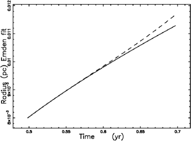
Figure 3: Theoretical radius as given by Eq. (21) (full line) and series solution as given by Eq. (24) (dashed line). Data as in Table 1.

The progenitor of SN 1993J was a K-supergiant star, see Aldering et al. (1994) and probably formed a binary system with an B-supergiant companion star, see Maund et al. (2004). These massive stars have strong stellar winds, and blow huge bubbles (of $\approx$ 20 to 40 pc in size) in their lives. From an analytic approximation Weaver et al. (1977) obtained a formula for the radius of the bubble, their eqn.(21), see too their Figure 3. The inner of the bubble has very low density, and the border of the bubble is the wall of a relatively dense shell which is in contact with the ISM. The circumstellar envelope of the Pre SN 1993J with which is interacting the SN shock front is a small structure within the big bubble created by the strong stellar winds of the SN progenitor (and probably of its binary companion) during its life. Therefore this envelope of the Pre SN 1993J would be the product of a recent event of stellar mass ejection suffered by the Pre SN 1993J . That is to say that the SN shock wave interacts with a CSM created by Pre supernova mass loss. In this respect, Schmidt et al. (1993) gave evidences that significant mass loss had taken place before the explosion, see also Smith (2008). In the scenario that the Pre SN 1993J formed an interacting binary system, this can be interpreted in terms of a process of mass transfer. It is possible that this type of supernova originates in interacting binary systems.

6.3 Two types of fit

The quality of the fits is measured by the merit function $\chi^{2}$

$$\chi^{2}=\sum_{j}\frac{(r_{th}-r_{obs})^{2}}{\sigma_{obs}^{2}}\quad,$$

where $r_{th}$, $r_{obs}$ and $\sigma_{obs}$ are the theoretical radius, the observed radius, and the observed uncertainty, respectively. A first fit can be done by assuming a power law dependence of the type

$$r(t)=r_{p}t^{\alpha_{p}}\quad,$$

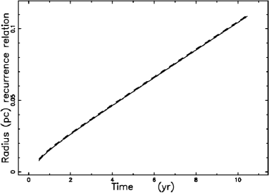
Figure 4: Theoretical radius as given by Eq. (21) (full line) and recursive solution as given by Eq. (27) when $\Delta t=0.05\mathrm{yr}$ (dashed line). Data as in Table 1.

where the two parameters $r_{p}$ and $\alpha_{p}$ as well their uncertainties can be found using the recipes suggested in Zaninetti (2011). A second fit can be done by assuming a piecewise function as in Fig. 4 of Marcaide et al. (2009)

$$r(t)=\{\begin{array}[]{ll}r_{br}(\frac{t}{t_{br}})^{\alpha_{1}}&\mbox{if $t\leq t_{br}$ }\\ r_{br}(\frac{t}{t_{br}})^{\alpha_{2}}&\mbox{if $t>t_{br}$. }\end{array}.$$

This type of fit requires the determination of four parameters: $t_{br}$ the break time, $r_{br}$ the radius of expansion at $t=t_{br}$, and the exponents $\alpha_{1}$ and $\alpha_{2}$ of the two phases. The parameters of these two fits as well the $\chi^{2}$ can be found in Table 1.

Table 1: Numerical values of the parameters of the fits and $\chi^{2}$; $N$ represents the number of free parameters.

$$\begin{array}[]{cccc}\hline\cr\hline\cr\vskip 3.0pt plus 1.0pt minus 1.0pt\cr N&values&\chi^{2}\\ \vskip 3.0pt plus 1.0pt minus 1.0pt\cr\hline\cr\vskip 3.0pt plus 1.0pt minus 1.0pt\cr&power~{}law~{}as~{}a~{}fit&&\\ \vskip 3.0pt plus 1.0pt minus 1.0pt\cr 2&\alpha_{p}=0.82\pm 0.0048&6364\\ \vskip 3.0pt plus 1.0pt minus 1.0pt\cr{}\hfil&r_{p}=(0.015\pm 0.00011)~{}{\mathrm{pc}}&\\ \vskip 3.0pt plus 1.0pt minus 1.0pt\cr\hline\cr&piecewise~{}fit&&\\ \vskip 3.0pt plus 1.0pt minus 1.0pt\cr 4&\alpha_{1}=0.83\pm 0.01&32\par\\ &\alpha_{2}=0.78\pm 0.0077;&{}\hfil\\ \vskip 3.0pt plus 1.0pt minus 1.0pt\cr{}\hfil&r_{br}=0.05~{}{\mathrm{pc}};t_{br}=4.10~{}{yr}&\\ \vskip 3.0pt plus 1.0pt minus 1.0pt\cr\hline\cr&Plummer~{}profile~{},\eta=6&&\\ \vskip 3.0pt plus 1.0pt minus 1.0pt\cr 2&b=0.0045~{}{\mathrm{pc}};r_{0}=0.008~{}{\mathrm{pc}};v_{0}=19500\frac{km}{s}&265\\ \vskip 3.0pt plus 1.0pt minus 1.0pt\cr\hline\cr&Lane--Emden~{}profile&&\\ \vskip 3.0pt plus 1.0pt minus 1.0pt\cr 2&b=0.00367~{}{\mathrm{pc}};r_{0}=0.008~{}{\mathrm{pc}};v_{0}=19500\frac{km}{s}&471\\ \vskip 3.0pt plus 1.0pt minus 1.0pt\cr\hline\cr&Power~{}law~{}profile&&\\ \vskip 3.0pt plus 1.0pt minus 1.0pt\cr 2&d=2.93;r_{0}=0.0022~{}{\mathrm{pc}};&276\\ \vskip 3.0pt plus 1.0pt minus 1.0pt\cr{}\hfil&t_{0}=0.249~{}{yr};v_{0}=100000\frac{km}{s}&{}\hfil\\ \vskip 3.0pt plus 1.0pt minus 1.0pt\cr\hline\cr\hline\cr\end{array}$$

6.4 The Lane–Emden case

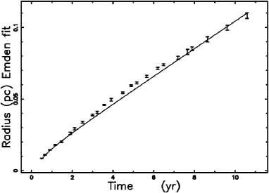
Figure 2: Theoretical radius as given by Eq. (21) (full line), with data as in Table 1. The astronomical data of SN 1993J are represented with vertical error bars.

The radius of SN 1993J which represents the momentum conservation in a Lane–Emden profile of density is reported in Fig. 2; $r_{0}$ and $t_{0}$ are fixed by the observations and the two free parameters are $b$ and $v_{0}$.

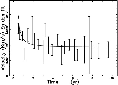
Figure 5: Instantaneous velocity of SN 1993J with uncertainty and theoretical velocity as given by Eq. (22) (full line). Data as in Table 1.

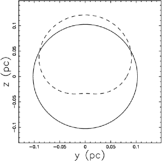
Figure 6: Sections of asymmetrical SN with the same initial parameters of SN 1993J in the plane which contains the center of the polytrope when $z_{asymm}=0$ pc (full line) and $z_{asymm}=-0.00367$ pc (dashed line). Data as in Table 1. In the asymmetrical case (dashed line) the degrees of asymmetry are $a_{up}=32\%$ and $a_{down}=32\%$, see formulae (28) and (29).

Fig. 3 compares the theoretical solution and the series expansion about the ordinary point $t_{0}$. The range of time in which the series solution approximates the analytical solution is limited. Fig. 4 compares the theoretical solution and the recursive solution as represented by Eq. 27. The recursive solution approximates the analytical solution over all the range of time considered and the error at $t=10$ yr is $\approx$ 0.6$\%$ when $\Delta t=0.05$ yr and $\approx$ 0.1$\%$ when $\Delta t=0.0083$ yr. The time evolution of the velocity is reported in Fig. 5. The asymmetrical case in which there is a distance, $z_{asymm}$, from the center of the polytrope and the center of the expansion is clearly outlined in Fig. 6. In this figure we have two sections of the expansion in the plane connecting $z_{asymm}$ with the center of the expansion with $z_{asymm}$ increasing from 0 (the circular section) to 0.00367 pc (the asymmetrical section).

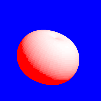
Figure 7: The 3D advancing surface of an asymmetrical SN with the same initial parameters of SN 1993J . The three Eulerian angles characterizing the point of view are $\Phi=70^{\circ}$, $\Theta=70^{\circ}$ and $\Psi=70^{\circ}$

Fig. 7 reports the complex structure of the 3D advancing surface. The point of view of the observer is parametrized by the Euler angles $(\Phi,\Theta,\Psi)$.

6.5 Plummer and power law cases

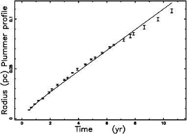
Figure 8: Theoretical radius for the Plummer-type profile as obtained by the solution of the nonlinear equation connected with (19) (full line). Data as in Table 1.

The numerical solution of the differential equation connected with the Plummer-like profile, $\eta=6$, is reported in Fig. 8 when the data of Table 1 are adopted.

A comparison with the power law behavior for the CSM is reported in Fig. 9 which is built from the data in Table 1. The series solution for the power law dependence of the CSM with coefficients as given by Eq. (31) is not reported because the range in time of reliability is limited to $t-t_{0}\approx 0.0003$ yr.

7 Relativistic astrophysical applications

We now apply the relativistic solutions derived so far to SN 1993J . The initial observed velocity, $v_{0}$, as deduced from radio observations, see Marcaide et al. (2009), is $v_{0}\approx 20000\,\rm\,{kms^{-1}}$ at $t_{0}\approx 0.5\,\mathrm{yr}$. We now reduce the initial time $t_{0}$ and we increase the velocity up to the relativistic regime, $t_{0}=10^{-4}\,\mathrm{yr}$, and $v_{0}=100000\,\rm\,{kms^{-1}}$. This choice of parameters allows fitting the observed radius–time relation that should be reproduced. The data used in the simulation are shown in Table 2.

Table 2: Numerical values of the parameters used in three relativistic solutions.

$$\begin{array}[]{c}\hline\cr\hline\cr\vskip 3.0pt plus 1.0pt minus 1.0pt\cr parameters\\ t_{0}=10^{-4}~{}\mathrm{yr}~{};r_{0}=0.0033~{}\mathrm{pc}~{};~{}\beta_{0}=0.3333~{};~{}b=0.004~{}\mathrm{pc}\\ \vskip 3.0pt plus 1.0pt minus 1.0pt\cr\hline\cr\end{array}$$

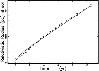
Figure 10: Theoretical relativistic radius as solution of the non-linear equation (33) (full line), with data as in Table 2.

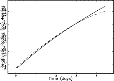
Figure 11: Theoretical relativistic radius as solution of the non-linear equation (33) (full line), and series solution as given by Eq. (34) (dashed line). Data as in Table 2. The time is expressed in days.

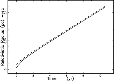
Figure 12: Theoretical relativistic radius as solution of the non-linear equation (33) (full line), and recursive solution as given by Eq. (5) when $\Delta t=0.053\mathrm{yr}$ (dashed line). Data as in Table 2.

The relativistic numerical solution of Eq. (33) is reported in Fig. 10, the relativistic series solution as given by (34) is reported in Fig. 11, and Fig. 12 contains the recursive solution as given by Eq. (5).

Fig. 13 reports a 2D map of the parameter $D$ which parametrizes the time dilation.

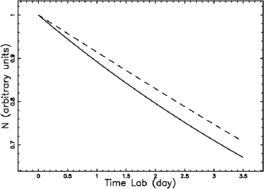
Figure 14: Number of nuclei of ⁵⁶Ni in the inertial frame of the laboratory (full line) and in the frame that is moving with the SN (dashed line). Data as in Table 2.

Fig. 14 reports the temporal evolution in the number of ⁵⁶Ni ($\tau$ = 8.757 d) in the laboratory frame at rest and in the frame which is moving with the SN. Fig. 15 reports the temporal evolution of the relativistic kinetic energy for a proton.

8 Conclusions

Classic Case: The thin layer approximation which models the expansion in an self-gravitating medium of the Lane–Emden type ($n=5$) can be modeled by a differential equation of the first order for the radius as a function of time. This differential equation has an analytical solution represented by Eq. (21). A power law series, see Eq. (24), can model the solution of the Lane–Emden type for a limited range of time, see Fig. 3. Conversely, a recursive solution for the first order differential equation, as represented by Eq. (27), approximates quite well the analytical solution of the Lane–Emden type and at the time of $t=10$ yr a precision of four digits is reached when $\Delta t=10^{-3}$ yr. The goodness of the results as given by the solutions of the three differential equations is evaluated in Table 1. The smallest $\chi^{2}$ is obtained by the Plummer-like ($\eta=6$) profile, followed by the power law profile and the Lane–Emden type ($n=5$) profile. The two-piece fit has the smallest $\chi^{2}$ but requires four parameters and does not have a physical basis. The disadvantages of the power law dependence in the CSM are: (i) there is a two-piece dependence at $r=r_{0}$ which was introduced in order to avoid a pole, (ii) there is no analytical solution, (iii) the series solution has a narrow range of reliability.

Auto-gravitating medium: The previous analysis raises a question: is the CSM around an SN really self-gravitating? In order to answer this question, the CSM should be carefully analyzed by astronomers in order to detect the presence of gradients in density or pressure or temperature. In the case of a Lane–Emden ($n=5$) CSM, the density of the medium around SN 1993J , see Eq. (8), decreases by a factor $\approx$ 21 going from $r_{0}=0.008$ pc to $r=0.1$ pc. Over the same distance, the pressure, see Eq. (6), decreases by a factor $\approx$ 40 and the temperature, see Eq. (7), by a factor $\approx$ 1.8. The presence or absence of a magnetic field should be also confirmed.

Nature of the CSM: The obtained total mass in the three models can be interpreted as the stellar mass ejected by the pre-SN right before the explosion or the stellar mass involved with the interaction of the binaries, see Table 3. The size of the pre-SN 1993J envelope, i.e. the FWHM, is an important data that could be related with the size of the Roche lobes of the hypothetical binary system, see Table 3.

Table 3: Numerical values of the swept total mass when $n_{0}=10^{7}\mathrm{cm}^{-3}$ and the FWHM. The parameter $n_{7}$ represents the number density expressed in $10^{7}\mathrm{cm}^{-3}$ units.

$$\begin{array}[]{ccc}\hline\cr\hline\cr\vskip 3.0pt plus 1.0pt minus 1.0pt\cr Model&Total~{}Mass&FWHM\\ \vskip 3.0pt plus 1.0pt minus 1.0pt\cr\hline\cr\vskip 3.0pt plus 1.0pt minus 1.0pt\cr Plummer~{}profile~{},\eta=6&M(0.1;0.0045)=0.402\,n_{7}\,M_{\sun}&0.0079~{}{\mathrm{pc}}\\ \vskip 3.0pt plus 1.0pt minus 1.0pt\cr Emden~{}profile&M(0.008;0.00367)=0.178\,n_{7}M_{\sun}&0.0071~{}{\mathrm{pc}}\\ \vskip 3.0pt plus 1.0pt minus 1.0pt\cr Emden~{}profile&M(0.1;0.00367)=0.368\,n_{7}M_{\sun}&0.0071~{}{\mathrm{pc}}\\ \vskip 3.0pt plus 1.0pt minus 1.0pt\cr Power~{}law~{}profile&M(0.1;0.0022,2.93)=0.217\,n_{7}M_{\sun}&0.0092~{}{\mathrm{pc}}\\ \vskip 3.0pt plus 1.0pt minus 1.0pt\cr\hline\cr\hline\cr\end{array}$$

Here we have chosen, in the three models, a central density of $n_{0}=10^{7}\mathrm{cm}^{-3}$. As a comparison Suzuki & Nomoto (1995), in order to model the X-ray observations, quotes a central density of $5.7\,10^{-4}g\mathrm{cm}^{-3}$ at a distance of $\approx 10^{-5}\mathrm{pc}$ which means $n_{0}=2.45\,10^{10}\mathrm{cm}^{-3}$. An astrophysical evaluation of $n_{7}$ can be done by imposing that the swept mass is a fraction $f$, $0<f<1$, of the mass of the progenitor which is $5\,M_{\sun}$, see Woosley et al. (1994); in the case of the Emden profile $n_{7}=13.57\,f$. With this evaluation the velocity dispersions to maintain the dynamic equilibrium, as given by formula (17), are of order $3.161\,\sqrt{f}\frac{km}{s}$. The previous table allows a fast evaluation of the final velocity, $v$, in the framework of the momentum conservation $v=v_{0}\frac{M(0.008;0.00367)}{M(0.1;0.00367)}=15437\frac{0.1778}{0.3686}\frac{km}{s}=7447\frac{km}{s}$.

Asymmetry: In the binary system scenario, both stars had probably a common envelope centered at the gravity center of the system. Hence, the SN exploded at a distance $\approx$ a/2 (assuming two stars of similar masses) with respect to the center of the density distribution of the CSM, where a is the distance between the stars of the binary system. In the case of SN 1993J the expansion shows a circular expansion over 10 years and the asymmetry is under $2\%$. This means, in the binary system scenario, that the distance, d, between initial point of the expansion and the center of the Lane–Emden ($n=5$) CSM should be $d\leq 0.037\,b$ or $d\leq 0.00013pc$. The distance a/2 is therefore equalized to our parameter d which means $a\leq 0.00026pc$.

Relativistic case: The temporal evolution of a SN in an self-gravitating medium of the Lane–Emden type can be found by applying the conservation of relativistic momentum in the thin layer approximation. This relativistic invariant is evaluated as a differential equation of the first order, see Eq. (32). Three different relativistic solutions for the radius as a function of time are derived: (i) a numerical solution, see Eq. (33) which covers the range $10^{-4}\mathrm{yr}<\,t<10\,\mathrm{yr}$ and fits the observed radius–time relation for SN 1993J ; (ii) a series solution, see Eq. (33), which has a limited range of validity, $10^{-4}\mathrm{yr}<\,t<1.2\times 10^{-2}\,\mathrm{yr}$; (iii) a recursive solution, see Eq. (5), in which the desired accuracy is reached by decreasing the time step $\Delta t$. The relativistic results here presented model SN 1993J and are obtained with an initial velocity of $v_{0}=100000\rm\,{kms^{-1}}$ or $\beta_{0}=0.333$ or $\gamma=1.06$. The time dilation is evaluated and then applied to the decay of ⁵⁶Ni, see Fig. 13. The relativistic kinetic energy of a proton is computed and the temporal evolution in Mev outlined, see Fig. 15.

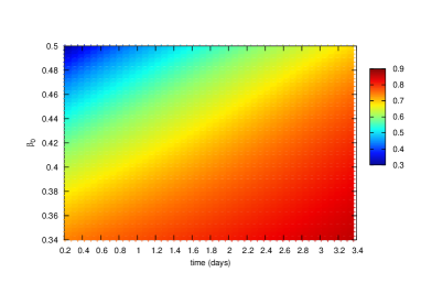
Figure 13: Map of time dilation as represented by $D$ as a function of time (in days) and $\beta_{0}$. Data as in Table 2.

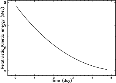
Figure 15: Relativistic kinetic energy of a proton in Mev as a function of time (in days). Data as in Table 2.

References

• Abramowitz & Stegun (1965) Abramowitz, M., & Stegun, I. A. 1965, Handbook of Mathematical Functions with Formulas, Graphs, and Mathematical Tables (New York: Dover)
• Aldering et al. (1994) Aldering, G., Humphreys, R. M., & Richmond, M. 1994, AJ , 107, 662
• Aoi et al. (2010) Aoi, J., Murase, K., Takahashi, K., Ioka, K., & Nagataki, S. 2010, ApJ  , 722, 440
• Baring (2011) Baring, M. G. 2011, Advances in Space Research, 47, 1427
• Bartel et al. (2007) Bartel, N., Bietenholz, M. F., Rupen, M. P., & Dwarkadas, V. V. 2007, ApJ  , 668, 924
• Beringer et al. (2012) Beringer, J., Arguin, J.-F., Barnett, R. M., & Copic, K. 2012, Phys. Rev. D , 86, 010001
• Bevington, P. R. and Robinson, D. K. (2003) Bevington, P. R. and Robinson, D. K. 2003, Data Reduction and Error analysis for the physical sciences (New York: McGraw-Hill)
• Binney & Tremaine (2011) Binney, J., & Tremaine, S. 2011, Galactic dynamics, Second Edition (Princeton, NJ: Princeton University Press)
• Blandford & McKee (1976) Blandford, R. D., & McKee, C. F. 1976, Physics of Fluids, 19, 1130
• Bodansky et al. (1968) Bodansky, D., Clayton, D. D., & Fowler, W. A. 1968, ApJS , 16, 299
• Chandrasekhar (1967) Chandrasekhar, S. 1967, An introduction to the study of stellar structure (New York)
• Chen et al. (2013) Chen, T.-W., Smartt, S. J., Bresolin, F., Pastorello, A., Kudritzki, R.-P., Kotak, R., McCrum, M., Fraser, M., & Valenti, S. 2013, ApJ  , 763, L28
• Chevalier (1982a) Chevalier, R. A. 1982a, ApJ  , 258, 790
• Chevalier (1982b) —. 1982b, ApJ  , 259, 302
• Childress et al. (2014) Childress, M. J., Filippenko, A. V., Ganeshalingam, M., & Schmidt, B. P. 2014, MNRAS  , 437, 338
• Dyson, J. E. and Williams, D. A. (1997) Dyson, J. E. and Williams, D. A. 1997, The physics of the interstellar medium (Bristol: Institute of Physics Publishing)
• Einstein (1905) Einstein, A. 1905, Annalen der Physik, 322, 891
• Elmhamdi et al. (2003) Elmhamdi, A., Chugai, N. N., & Danziger, I. J. 2003, A&A  , 404, 1077
• Emden (1907) Emden, R. 1907, Gaskugeln: anwendungen der mechanischen warmetheorie auf kosmologische und meteorologische probleme (Berlin: B. Teubner.)
• Eriksen et al. (2009) Eriksen, K. A., Arnett, D., McCarthy, D. W., & Young, P. 2009, ApJ  , 697, 29
• French, A.P. (1968) French, A.P. 1968, Special Relativity (New York: CRC)
• Frisch & Smith (1963) Frisch, D. H., & Smith, J. H. 1963, American Journal of Physics, 31, 342
• Granot & Kumar (2006) Granot, J., & Kumar, P. 2006, MNRAS  , 366, L13
• Guéry-Odelin & Lahaye (2010) Guéry-Odelin, D., & Lahaye, T. 2010, Classical Mechanics Illustrated by Modern Physics: 42 Problems with Solutions (London: Imperial College Press)
• Hansen & Kawaler (1994) Hansen, C. J., & Kawaler, S. D. 1994, Stellar Interiors. Physical Principles, Structure, and Evolution. (Berlin: Springer-Verlag)
• Ince (2012) Ince, E. L. 2012, Ordinary differential equations (New York: Courier Dover Publications)
• Inoue et al. (2011) Inoue, T., Asano, K., & Ioka, K. 2011, ApJ  , 734, 77
• Kashiyama et al. (2013) Kashiyama, K., Murase, K., Horiuchi, S., Gao, S., & Mészáros, P. 2013, ApJ  , 769, L6
• Kocevski & Petrosian (2013) Kocevski, D., & Petrosian, V. 2013, ApJ  , 765, 116
• Kompaneyets (1960) Kompaneyets, A. S. 1960, Soviet Phys. Dokl., 5, 46
• Krisciunas et al. (2011) Krisciunas, K., Li, W., Matheson, T., Howell, D. A., Stritzinger, M., Aldering, G., Berlind, P. L., Calkins, M., Challis, P., Chornock, R., Conley, A., Filippenko, A. V., Ganeshalingam, M., Germany, L., González, S., Gooding, S. D., Hsiao, E., Kasen, D., Kirshner, R. P., Howie Marion, G. H., Muena, C., Nugent, P. E., Phelps, M., Phillips, M. M., Qiu, Y., Quimby, R., Rines, K., Silverman, J. M., Suntzeff, N. B., Thomas, R. C., & Wang, L. 2011, AJ , 142, 74
• Lane (1870) Lane, H. J. 1870, American Journal of Science, 148, 57
• Larmor (1897) Larmor, J. 1897, Philos. Trans. R. Soc. Lond., Ser. A, Contain. Pap. Math. Phys. Character, 190, 205
• Lorentz (1904) Lorentz, H. A. 1904, in Proc. Acad. Sciences Amsterdam, Vol. 6, 809–830
• Lyutikov (2012) Lyutikov, M. 2012, MNRAS  , 421, 522
• Macrossan (1986) Macrossan, M. N. 1986, The British journal for the philosophy of science, 37, 232
• Magkotsios et al. (2010) Magkotsios, G., Timmes, F. X., Hungerford, A. L., Fryer, C. L., Young, P. A., & Wiescher, M. 2010, ApJS , 191, 66
• Marcaide et al. (2009) Marcaide, J. M., Martí-Vidal, I., Alberdi, A., & Pérez-Torres, M. A. 2009, A&A  , 505, 927
• Marion et al. (2013) Marion, G. H., Vinko, J., & Wheeler, J. C. 2013, ApJ  , 777, 40
• Matz & Share (1990) Matz, S. M., & Share, G. H. 1990, ApJ  , 362, 235
• Maund et al. (2004) Maund, J. R., Smartt, S. J., Kudritzki, R. P., Podsiadlowski, P., & Gilmore, G. F. 2004, Nature  , 427, 129
• Mazzali et al. (2005) Mazzali, P. A., Benetti, S., Altavilla, G., Blanc, G., & Cappellaro, E. 2005, ApJ  , 623, L37
• Mazzali et al. (1997) Mazzali, P. A., Chugai, N., Turatto, M., Lucy, L. B., Danziger, I. J., Cappellaro, E., della Valle, M., & Benetti, S. 1997, MNRAS  , 284, 151
• McCray (1987) McCray, R. A. 1987, in Spectroscopy of Astrophysical Plasmas, ed. A. Dalgarno & D. Layzer, 255–278
• Mohr et al. (2012) Mohr, P. J., Taylor, B. N., & Newell, D. B. 2012, Reviews of Modern Physics, 84, 1527
• Muccino et al. (2013) Muccino, M., Ruffini, R., Bianco, C. L., & Izzo, L. 2013, ApJ  , 772, 62
• Nakar & Sari (2012) Nakar, E., & Sari, R. 2012, ApJ  , 747, 88
• Okita et al. (2012) Okita, S., Umeda, H., & Yoshida, T. 2012, in American Institute of Physics Conference Series, Vol. 1484, American Institute of Physics Conference Series, ed. S. Kubono, T. Hayakawa, T. Kajino, H. Miyatake, T. Motobayashi, & K. Nomoto, 418–420
• Olano (2009) Olano, C. A. 2009, A&A  , 506, 1215
• Olver et al. (2010) Olver, F. W. J. e., Lozier, D. W. e., Boisvert, R. F. e., & Clark, C. W. e. 2010, NIST handbook of mathematical functions. (Cambridge: Cambridge University Press. )
• Padmanabhan (2001) Padmanabhan, P. 2001, Theoretical astrophysics. Vol. II: Stars and Stellar Systems (Cambridge, UK: Cambridge University Press)
• Pe’er et al. (2007) Pe’er, A., Ryde, F., Wijers, R. A. M. J., & Mészáros, P. 2007, ApJ  , 664, L1
• Plummer (1911) Plummer, H. C. 1911, MNRAS  , 71, 460
• Rossi & Hall (1941) Rossi, B., & Hall, D. B. 1941, Physical Review, 59, 223
• Schmidt et al. (1993) Schmidt, B. P., Kirshner, R. P., Eastman, R. G., Grashuis, R., dell’Antonio, I., Caldwell, N., Foltz, C., Huchra, J. P., & Milone, A. A. E. 1993, Nature  , 364, 600
• Sedov (1959) Sedov, L. I. 1959, Similarity and Dimensional Methods in Mechanics (New York: Academic Press)
• Shapiro (1979) Shapiro, P. R. 1979, ApJ  , 233, 831
• Smith (2008) Smith, N. 2008, in Revista Mexicana de Astronomia y Astrofisica Conference Series, Vol. 33, Revista Mexicana de Astronomia y Astrofisica Conference Series, 154–156
• Spitzer (1978) Spitzer, L. 1978, Physical processes in the interstellar medium (New-York: Wiley)
• Stritzinger et al. (2006) Stritzinger, M., Leibundgut, B., Walch, S., & Contardo, G. 2006, A&A  , 450, 241
• Suzuki & Nomoto (1995) Suzuki, T., & Nomoto, K. 1995, ApJ  , 455, 658
• Tenenbaum & Pollard (1963) Tenenbaum, M., & Pollard, H. 1963, Ordinary Differential Equations: An Elementary Textbook for Students of Mathematics, Engineering, and the Sciences (New York: Dover Publications)
• Truran et al. (1967) Truran, J. W., Arnett, W. D., & Cameron, A. G. W. 1967, Canadian Journal of Physics, 45, 2315
• Truran et al. (2012) Truran, J. W., Glasner, A. S., & Kim, Y. 2012, Journal of Physics Conference Series, 337, 012040
• Wang et al. (2003) Wang, L., Baade, D., Hoflich, P., Khokhlov, A., & Wheeler, J. C. 2003, ApJ  , 591, 1110
• Weaver et al. (1977) Weaver, R., McCray, R., Castor, J., Shapiro, P., & Moore, R. 1977, ApJ  , 218, 377
• Whitworth & Ward-Thompson (2001) Whitworth, A. P., & Ward-Thompson, D. 2001, ApJ  , 547, 317
• Woosley et al. (1994) Woosley, S. E., Eastman, R. G., Weaver, T. A., & Pinto, P. A. 1994, ApJ  , 429, 300
• Zaninetti (2011) Zaninetti, L. 2011, Astrophysics and Space Science , 333, 99
• Zaninetti (2012) Zaninetti, L. 2012, Central European Journal of Physics, 10, 32
• Zhang et al. (2013) Zhang, F.-W., Fan, Y.-Z., Shao, L., & Wei, D.-M. 2013, ApJ  , 778, L11
• Zhang (1997) Zhang, Y. 1997, Special Relativity and Its Experimental Foundations (Singapore: World Scientific)
• Zou & Piran (2010) Zou, Y.-C., & Piran, T. 2010, MNRAS  , 402, 1854
• Zwillinger (1989) Zwillinger, D. 1989, Handbook of differential equations (New York: Academic Press)
Refer to caption