Unification of SUSY breaking and GUT breaking

Abstract

We build explicit supersymmetric unification models where grand unified gauge symmetry breaking and supersymmetry (SUSY) breaking are caused by the same sector. Besides, the SM-charged particles are also predicted by the symmetry breaking sector, and they give the soft SUSY breaking terms through the so-called gauge mediation. We investigate the mass spectrums in an explicit model with $SU(5)$ and additional gauge groups, and discuss its phenomenological aspects. Especially, nonzero A-term and B-term are generated at one-loop level according to the mediation via the vector superfields, so that the electro-weak symmetry breaking and $125$ GeV Higgs mass may be achieved by the large B-term and A-term even if the stop mass is around $1$ TeV.

I Introduction

As well-known, the Standard Model (SM) is very successful in describing our nature, and it is firmly established by the Higgs discovery at the LHC Higgs . There are still some ambiguities in not only the signal strength of the Higgs particle but also the other observations such as flavor physics, but it would be getting more difficult to consider new-physics effects in any signals.

On the other hand, we are sure that the SM remains several mysteries about our nature: the origin of the fermion generations, the hyper-charge assignment, the Higgs mass, and so on. Many Beyond Standard Models (BSM) were proposed so far motivated by those mysteries, and some of them are expected to be found near future. One of the candidates is the supersymmetric grand unified theory (GUT), which reveals the origin of the Higgs mass and the fermion charges. There are some issues in Yukawa couplings, for instance, how to generate realistic Yukawa couplings and heavy colored Higgs, but it succeeds in the charge quantization ($|Q_{e}+Q_{p}|<10^{-21}$ PDG ) and naturally deriving the electro-weak (EW) scale, if the supersymmetry (SUSY) scale $(\Lambda_{SUSY})$ is close to the EW scale. The supersymmetric GUT scenario is constrained by the observation of the proton decay, the direct search of SUSY particles, and the SM measurements. Especially, the Higgs discovery around $125$ GeV may require high-scale SUSY $(\Lambda_{SUSY}\gg O(1){\rm TeV})$ Higgs1 , which may discard the strong motivation of SUSY, that is, the natural explanation of the EW scale. Furthermore, the gauge coupling unification of supersymmetric $SU(5)$ GUT might be lost in high-scale SUSY, depending on the mass spectrum of the SUSY particles. The supersymmetric models could have so many parameters in the bottom-up approach, so that we could have some solutions for the Higgs mass and the gauge coupling unification. However, it is very important to find how to derive such a specific SUSY mass spectrum.

In this paper, we propose an explicit supersymmetric GUT with $SU(5)_{F}\times SU(2)\times U(1)_{\phi}$ gauge groups. We discard the miracle of the gauge coupling unification in the Minimal Supersymmetric SM (MSSM), but SUSY breaking and GUT breaking sectors are unified. The SM-charged particles also appear after the symmetry breaking, so the messenger fields for the gauge mediation is also introduced by the breaking sector in our model. The SM fields are only charged under the $SU(5)_{F}$ gauge group, so that the charge quantization is realized.

The breaking sector consists of one $SU(5)_{F}$ adjoint plus singlet filed $(\Phi)$ and $SU(5)_{F}$ fundamental and anti-fundamental fields $(\phi,~{}\widetilde{\phi})$. The vector-like pairs $(\phi,~{}\widetilde{\phi})$ are also charged under $SU(2)\times U(1)_{\phi}$. As discussed in Ref. ISS , this type of gauge theory causes SUSY breaking along with the gauge symmetry breaking. In our model, $SU(5)_{F}\times SU(2)\times U(1)_{\phi}$ symmetry breaks down to the SM gauge groups, $SU(3)_{c}\times SU(2)_{L}\times U(1)_{Y}$, where $SU(3)_{c}$ is from the subgroup of $SU(5)_{F}$, and $SU(2)_{L}\times U(1)_{Y}$ are the linear combinations of the subgroup of $SU(5)_{F}$ and $SU(2)\times U(1)_{\phi}$. SUSY is broken by the F-component of the part of $\Phi$. After the symmetry breaking, SM-charged particles are generated by the fluctuation of $\Phi$ and $(\phi,~{}\widetilde{\phi})$ around the vacuum expectation values (VEVs). One interesting point is that the massive gauge boson of $SU(5)_{F}$ and the fermionic partners could mediate the SUSY breaking effect through the gauge coupling with $\Phi$, and play a crucial role in generating the non-zero A-term and B-term as discussed in Refs.Dermisek ; Matos . It is well-known that SUSY-scale A-term could shift the upper bound on the lightest Higgs mass in the MSSM, even if squark is light, and the SUSY-scale B-term is required to realize the EW symmetry breaking. Our A-term and B-term are given at one-loop level, so that they are the same order as the squark masses and gaugino masses. In fact, we will see that Higgs mass could be around $125$ GeV, even if $\Lambda_{SUSY}$ is less than $O(1)$ TeV, and the B-term could be consistent with the EW symmetry breaking.

In Sec. II, we introduce the SUSY and GUT breaking sector in generic $SU(N_{F})_{F}\times SU(N)\times U(1)_{\phi}$ gauge theory. There, we discuss not only the symmetry breaking, but also the behavior of the gauge couplings and soft SUSY breaking terms according to the gauge mediation with the mediators of the chiral superfields and the vector superfields. In Sec. III, we apply the breaking sector to the $SU(5)_{F}\times SU(2)\times U(1)_{\phi}$ gauge theory. As we mentioned above, an interesting aspect of this model is the improvement of the consistency with the EW symmetry breaking and Higgs mass in the case with low-scale SUSY. We investigate the soft SUSY breaking terms, and discuss how well it is achieved in our scenario. In Sec. IV, we give a comment on the possibility that the breaking sector is applied to other GUT models. Sec. V is devoted to the summary. In Appendix A, we give the mass spectrum in the SUSY breaking sector. In Appendix B, we show examples of mass spectrums in the MSSM sector.

II $SU(N)\times SU(N_{F})_{F}\times U(1)_{\phi}$ gauge theory

In this section, we introduce the model which causes SUSY breaking together with gauge symmetry breaking, based on Ref. ISS .

We consider $SU(N_{F})_{F}\times SU(N)\times U(1)_{\phi}$ gauge theory with $N_{F}>N$. The matter content is shown in Table 1: $\Phi$ is the $SU(N_{F})_{F}$ adjoint plus singlet field and $(\phi,\widetilde{\phi})$ pair is the vector-like under $SU(N_{F})_{F}\times SU(N)\times U(1)_{\phi}$ gauge group.

	$\phi$	$\widetilde{\phi}$	$\Phi$
$SU(N_{F})_{F}$	${\bf N_{F}}$	$\overline{{\bf N_{F}}}$	adj${}_{N_{F}}$+1
$SU(N)$	$\overline{{\bf N}}$	${\bf N}$	1
$U(1)_{\phi}$	$Q_{\phi}$	$-Q_{\phi}$	0

Table 1: Chiral superfields in $SU(N_{F})_{F}\times SU(N)\times U(1)_{\phi}$ gauge theory

The superpotential is given by

$$W_{R}=-hTr_{N}(\widetilde{\phi}\Phi\phi)+h\Lambda_{G}{\rm Tr}_{N_{F}}(\Phi),$$ (1)

assigning $U(1)_{R}$ symmetry: the R-charge of $\Phi$ is $2$ and the R-charge of $(\phi,\widetilde{\phi})$ is vanishing. However, there would be an issue about how to break R-symmetry and how to avoid the massless particle according the $U(1)_{R}$ symmetry breaking. Let us introduce explicit $U(1)_{R}$ breaking terms,

$$W_{\not{R}}=m_{\phi}Tr_{N}(\widetilde{\phi}\phi)+c,$$ (2)

and discuss the superpotential as $W_{SB}=W_{R}+W_{\not{R}}$. In Ref. ISS , $W_{R}$ is generated, considering the dual side of $SU(N_{F})_{F}\times SU(N+N_{F})$ gauge theory with the $N_{F}$ vector-like pairs $(q_{d},\widetilde{q}_{d})$ of $SU(N+N_{F})$ gauge group. $\Phi$ is interpreted as the composite operator as $\Phi\equiv\widetilde{q}_{d}q_{d}$, and $h\Lambda_{G}{\rm Tr}_{N_{F}}(\Phi)$ in $W_{R}$ corresponds to the mass term of the $(q_{d},\widetilde{q}_{d})$.

Some ideas to induce $W_{\not{R}}$ have been proposed in Ref. AKO1 , where the small wave-function factor of $\Phi$ suppresses $\Phi^{2}$ and $\Phi^{3}$ terms according to the strong dynamics or the profile in the extra dimension. In Ref.AKO2 , the effect of the explicit R-symmetry breaking terms is well studied. Here, we simply start the discussion from the superpotential $W_{SB}$ assuming that such a mechanism, as discussed in Ref. AKO1 , works in underlying theories above the GUT, and study the symmetry breaking. In the global SUSY with canonical Kähler potential, the scalar potential is given by $V=|\partial_{\Phi}W_{SB}|^{2}+|\partial_{\phi}W_{SB}|^{2}+|\partial_{\widetilde{\phi}}W_{SB}|^{2}$, and SUSY vacua satisfy $\partial_{\Phi}W_{SB}=\partial_{\phi}W_{SB}=\partial_{\widetilde{\phi}}W_{SB}=0$. In this model, $\partial_{\Phi}W_{SB}$ is given by

$$\partial_{\Phi_{ji}}W_{SB}=-h(\phi\widetilde{\phi})_{ij}+h\Lambda_{G}\delta_{ij},$$ (3)

and all elements cannot be vanishing, because $N_{F}\times N_{F}$ matrix $(\phi\widetilde{\phi})$ has the rank $N$ $(<N_{F})$. This means that SUSY is broken by the F-components of $(N_{F}-N)$ elements in $\Phi$ and $SU(N_{F})_{F}$ would be also broken.

Following Ref. ISS , we decompose $\Phi$ and $(\phi,\tilde{\phi})$ as

$$\Phi = \left(\begin{array}[]{cc}\left(v_{Y}\right){\bf 1}_{N}+\hat{Y}&\widetilde{Z}\\ Z&\left(v_{X}\right){\bf 1}_{\widetilde{N}}+\hat{X}\end{array}\right),$$ (6)

$$\phi = \left(\begin{array}[]{c}\left(v_{\chi}\right){\bf 1}_{N}+\hat{\chi}\\ \rho\end{array}\right),\widetilde{\phi}^{T}=\left(\begin{array}[]{cc}\left(v_{\chi}\right){\bf 1}_{N}+\hat{\widetilde{\chi}}^{T}\\ \widetilde{\rho}^{T}\end{array}\right),$$ (11)

where $\hat{Y}$, $\hat{\chi}$ and $\hat{\tilde{\chi}}$ are $N\times N$ matrices, $\hat{X}$ is an $\widetilde{N}\times\widetilde{N}$ matrix ($\widetilde{N}=N_{F}-N$), $Z$ and $\rho$ ($\widetilde{Z}$ and $\widetilde{\rho}$) are $N\times\widetilde{N}$ matrices ($\widetilde{N}\times N$ matrices). The VEVs, $v_{Y}$ and $v_{\chi}$, are fixed by the stationary conditions

$$v_{Y} = \frac{m_{\phi}}{h},$$ (12)

$$v_{\chi} = \Lambda_{G}.$$ (13)

This solution also satisfies the D-flat conditions. $v_{X}$ is a flat direction in global SUSY. If we consider gravity and one-loop corrections, it would be stabilized at the nonzero value ISS ; AHKO .

The nonzero VEVs break $SU(N)\times SU(N_{F})_{F}\times U(1)_{\phi}$ gauge symmetry to $SU(\widetilde{N})\times SU(N)_{D}\times U(1)_{Y}$. $SU(N)_{D}$ and $U(1)_{Y}$ are the linear combinations of the subgroups of $SU(N_{F})_{F}$ and $SU(N)\times U(1)_{\phi}$.

II.1 gauge bosons

After the symmetry breaking, massive gauge bosons appear according to the Higgs mechanism. Let us decompose the vector field $(V^{\mu}_{F})$ for $SU(N_{F})_{F}$ as

$$V^{\mu}_{F} = \begin{pmatrix}W^{\mu}_{F}-aB^{\prime\mu}&&\frac{1}{\sqrt{2}}(X^{\mu})^{\dagger}\\ \frac{1}{\sqrt{2}}X^{\mu}&&G^{\mu}+\frac{N}{\widetilde{N}}aB^{\prime\mu}\end{pmatrix},$$ (14)

where $a=\frac{\sqrt{\widetilde{N}}}{\sqrt{2N(N+\widetilde{N})}}$ is defined. $W^{\mu}_{F}$ and $G^{\mu}$ are the adjoint representations of the subgroups of $SU(N_{F})_{F}$: $SU(N)_{F}$ and $SU(\widetilde{N})$. $X_{\mu}$ is the anti-fundamental and fundamental representations of $SU(N)_{F}\times SU(\widetilde{N})$, and $B^{\prime}_{\mu}$ is the $U(1)_{F}$ vector field, where $U(1)_{F}$ is from $SU(N_{F})_{F}$.

The nonzero VEVs generate the following mass terms,

$${\cal L}_{g} = M^{2}_{X}X^{\dagger}_{\mu}X^{\mu}+\frac{1}{2}M^{2}_{W^{\prime}}W^{\prime A}_{\mu}W^{\prime A\mu}+\frac{1}{2}M^{2}_{Z^{\prime}}Z^{\prime}_{\mu}Z^{\prime\mu},$$ (15)

$$M^{2}_{X} = g^{2}_{F}(v^{2}_{\chi}+\Delta v^{2}),$$ (16)

$$M^{2}_{W^{\prime}} = 2(g^{2}_{F}+g^{\prime 2}_{N})v^{2}_{\chi},$$ (17)

$$M^{2}_{Z^{\prime}} = 4N(Q^{2}_{\phi}g^{2}_{\phi}+a^{2}g_{F}^{2})v^{2}_{\chi},$$ (18)

where $\Delta v=v_{X}-v_{Y}$ is defined. $W^{\prime A\mu}$ and $Z^{\prime\mu}$ are given by the linear combinations of $W^{A\mu}_{F}$ and $SU(N)$ gauge boson ($W^{A\mu}_{N}$), and $B^{\prime\mu}$ and $U(1)_{\phi}$ gauge boson ($A^{\mu}_{\phi}$) respectively:

$$\begin{pmatrix}B^{\prime\mu}\\ A^{\mu}_{\phi}\end{pmatrix} = \begin{pmatrix}\cos\theta_{Y}&&\sin\theta_{Y}\\ -\sin\theta_{Y}&&\cos\theta_{Y}\end{pmatrix}\begin{pmatrix}B^{\mu}\\ Z^{\prime\mu}\end{pmatrix},$$ (19)

$$\begin{pmatrix}W^{A\mu}_{F}\\ W^{A\mu}_{N}\end{pmatrix} = \begin{pmatrix}\cos\theta&&-\sin\theta\\ \sin\theta&&\cos\theta\end{pmatrix}\begin{pmatrix}W^{A\mu}\\ W^{\prime A\mu}\end{pmatrix},$$ (20)

where $\cos\theta_{Y}$ and $\cos\theta$ are defined as

$$\cos\theta_{Y}=\frac{Q_{\phi}g_{\phi}}{\sqrt{Q_{\phi}^{2}g_{\phi}^{2}+a^{2}g_{F}^{2}}},~{}\cos\theta=\frac{g^{\prime}_{N}}{\sqrt{g^{\prime 2}_{N}+g_{F}^{2}}}.$$ (21)

$G_{\mu}$, $W_{\mu}$, and $B_{\mu}$ are the gauge bosons for $SU(\widetilde{N})\times SU(N)_{D}\times U(1)_{Y}$ gauge symmetry, and their gauge couplings are given by

$$g_{N}=g_{F}\cos\theta,~{}g_{\widetilde{N}}=g_{F},~{}g^{\prime}_{1}=aNg_{1}=aNg_{F}\cos\theta_{Y}.$$ (22)

II.2 SM-charged fields from symmetry breaking sector

According to the decomposition in Eqs. (6) and (11), we introduce the charge assignment of $(Z,\widetilde{Z})$, $(\rho,\widetilde{\rho})$, $Y$, $(\chi,\widetilde{\chi})$, and $X$ in Table 2. $Y$, $(\chi,\widetilde{\chi})$, and $X$ are the adjoint parts of $\hat{Y}$, $(\hat{\chi},\hat{\widetilde{\chi}})$, and $\hat{X}$. The singlet parts are not charged under the SM, and they are not so relevant to our analysis. The mass matrices are studied in Appendix A.

	$Z$	$\widetilde{Z}$	$\rho$	$\widetilde{\rho}$	$Y$	$\chi$	$\widetilde{\chi}$	$X$
$SU(\widetilde{N})$	$\widetilde{{\bf N}}$	$\overline{\widetilde{{\bf N}}}$	$\widetilde{{\bf N}}$	$\overline{\widetilde{{\bf N}}}$	1	1	1	adj${}_{\widetilde{N}}$
$SU(N)_{D}$	$\overline{{\bf N}}$	${\bf N}$	$\overline{\bf N}$	${\bf N}$	adjN	adjN	adjN	1
$U(1)_{Y}$	$\frac{N+\widetilde{N}}{N\widetilde{N}}$	$\frac{-N-\widetilde{N}}{N\widetilde{N}}$	$\frac{N+\widetilde{N}}{N\widetilde{N}}$	$\frac{-N-\widetilde{N}}{N\widetilde{N}}$	0	0	0	0

Table 2: Extra Chiral superfields charged under the $SU(\widetilde{N})\times SU(N)_{D}\times U(1)_{Y}$.

These fields obtain masses according to the nonzero VEVs, $v_{\chi}$, $v_{Y}$ and $v_{X}$ as we see in the Appendix A. They decouple at some scales above the EW scale. In the next subsection, we investigate the RG flows of the gauge couplings including the threshold corrections and discuss the soft SUSY breaking terms mediated by the heavy fields.

II.3 RG flows of the gauge couplings

In this model, two kinds of symmetry breaking actually happen: one is $SU(N_{F})_{F}$ breaking, $SU(N_{F})_{F}\to SU(\widetilde{N})\times SU(N)_{F}\times U(1)_{F}$, and the other is $SU(N)_{F}\times U(1)_{F}\times SU(N)\times U(1)_{\phi}$ breaking: $SU(N)_{F}\times SU(N)\to SU(N)_{D}$ and $U(1)_{F}\times U(1)_{\phi}\to U(1)_{Y}$. The former is caused by $\Delta v$, and the later is by $v_{\chi}$. We consider a simple scenario assuming $\Delta v\gg v_{\chi}$.

As we see in Appendix A, there will be several intermediate scales, where heavy particles in the symmetry breaking sector are decoupled and the RG flow of gauge couplings is modify. According to the one-loop RG equations, the gauge couplings at the EW scale ($M_{Z}$) are evaluated as follows: $SU(N)_{F}$, $SU(N)$ and $SU(N)_{D}$ gauge couplings $(\alpha_{F_{N}},\alpha^{\prime}_{N},\alpha_{N})$ are

$$4\pi\alpha^{-1}_{N}(M_{Z}) = 4\pi\alpha^{-1}_{F_{N}}(T_{\chi_{N}})+4\pi\alpha^{\prime-1}_{N}(T_{\chi_{N}})+b_{N}\ln\left(\frac{M_{Z}^{2}}{T^{2}_{\chi_{N}}}\right)+\Delta b^{N}_{\rm ex}\left(\frac{T_{\rm ex}^{2}}{\Lambda^{2}}\right),$$ (23)

$$4\pi\alpha^{-1}_{F_{N}}(T_{\chi_{N}}) = 4\pi\alpha^{-1}_{G}(\Lambda)+\Delta b_{N}\ln\left(\frac{T_{N}^{2}}{\Lambda^{2}}\right)+(b_{N}-2N)\ln\left(\frac{T_{\chi_{N}}^{2}}{\Lambda^{2}}\right),$$ (24)

$$4\pi\alpha^{\prime-1}_{N}(T_{\chi_{N}}) = 4\pi\alpha^{\prime-1}_{N}(\Lambda)+\Delta b_{\rho_{N}}\ln\left(\frac{T_{\rho_{N}}^{2}}{\Lambda^{2}}\right)-N\ln\left(\frac{T_{\chi_{N}}^{2}}{\Lambda^{2}}\right).$$ (25)

$SU(\widetilde{N})$ gauge coupling $(\alpha_{\widetilde{N}})$ is

$$4\pi\alpha^{-1}_{\widetilde{N}}(M_{Z}) = 4\pi\alpha^{-1}_{G}(\Lambda)+b_{\widetilde{N}}\ln\left(\frac{M_{Z}^{2}}{\Lambda^{2}}\right)+\Delta b_{\widetilde{N}}\ln\left(\frac{T_{\widetilde{N}}^{2}}{\Lambda^{2}}\right)$$

$$+ \Delta b^{\widetilde{N}}_{\rm ex}\ln\left(\frac{T_{\rm ex}^{2}}{\Lambda^{2}}\right)+\Delta b_{\rho_{\widetilde{N}}}\ln\left(\frac{T_{\rho_{\widetilde{N}}}^{2}}{\Lambda^{2}}\right)+\Delta b_{X}\ln\left(\frac{T_{\chi_{\widetilde{N}}}^{2}}{\Lambda^{2}}\right).$$

$U(1)_{F}$, $U(1)_{\phi}$, and $U(1)_{Y}$ gauge couplings $(\alpha_{F_{1}},\alpha_{\phi},\alpha_{1})$ are

$$4\pi\alpha^{-1}_{1}(M_{Z}) = 4\pi\alpha^{-1}_{F_{1}}(T_{\chi_{1}})+\frac{4\pi a^{2}}{Q_{\phi}^{2}}\alpha^{-1}_{\phi}(T_{\chi_{1}})+b_{1}\ln\left(\frac{M_{Z}^{2}}{T^{2}_{\chi_{1}}}\right)+\Delta b^{1}_{\rm ex}\ln\left(\frac{T_{\rm ex}^{2}}{\Lambda^{2}}\right),$$ (27)

$$4\pi\alpha^{-1}_{F_{1}}(T_{\chi_{1}}) = 4\pi\alpha^{-1}_{G}(\Lambda)+\Delta b_{1}\ln\left(\frac{T_{1}^{2}}{\Lambda^{2}}\right)+\Delta b_{\rho_{1}}\ln\left(\frac{T_{\rho_{1}}^{2}}{\Lambda^{2}}\right)+(b_{1}+\Delta b_{\chi_{1}})\ln\left(\frac{T_{\chi_{1}}^{2}}{\Lambda^{2}}\right),$$ (28)

$$4\pi\alpha^{-1}_{\phi}(T_{\chi_{1}}) = 4\pi\alpha^{-1}_{\phi}(\Lambda)+\Delta b_{\rho_{\phi}}\ln\left(\frac{T_{\rho_{1}}^{2}}{\Lambda^{2}}\right)+\Delta b_{\chi_{\phi}}\ln\left(\frac{T_{\chi_{1}}^{2}}{\Lambda^{2}}\right).$$

$\Lambda$ is the cut-off scale and $T_{i}$, $T_{\chi_{i}}$ and $T_{\rho_{i}}$ $(i=N,\widetilde{N},1)$ are the intermediate scales where $X_{\mu}$, $\chi_{i}(\chi_{\widetilde{N}}\equiv X)$, and $\rho_{i}$ decouple respecitvely. According to the mass spectrums at each scale in Appendix A, $T_{i}$, $T_{\chi_{i}}$ and $T_{\rho_{i}}$ $(i=N,\widetilde{N},1)$ are estimated as

$$(T_{N},T_{\rho_{N}},T_{\chi_{N}}) = (M_{X},h\Delta v,\sqrt{h}M_{G^{\prime}}),$$ (30)

$$(T_{\widetilde{N}},T_{\rho_{\widetilde{N}}},T_{\chi_{\widetilde{N}}}) = (M_{X},h\Delta v,m_{X}),$$ (31)

$$(T_{1},T_{\rho_{1}},T_{\chi_{1}}) = (M_{X},h\Delta v,\sqrt{h}M_{Z^{\prime}}).$$ (32)

The factor in front of each intermediate scale describes the freedom of the particles decoupling at the scale:

$$(\Delta b_{N},\Delta b_{\rho_{N}}) = (2(N_{F}-N),-\widetilde{N}),$$ (33)

$$(\Delta b_{\widetilde{N}},\Delta b_{\rho_{\widetilde{N}}},\Delta b_{X}) = (2(N_{F}-\widetilde{N}),-N,-\widetilde{N}),$$ (34)

$$(\Delta b_{1},\Delta b_{\rho_{1}},\Delta b_{\chi_{1}}) = \left(2N_{F},-a^{2}N^{2}\frac{2N}{\widetilde{N}},-2a^{2}N^{2}\right),$$ (35)

$$(\Delta b_{\rho_{\phi}},\Delta b_{\chi_{\phi}}) = (-2N\widetilde{N}Q^{2}_{\phi},-2N^{2}Q^{2}_{\phi}).$$ (36)

We may also have to introduce additional particles charged under the gauge symmetry, in order to achieve realistic mass spectrums. For instance, colored Higgs would be necessary to derive the MSSM Higgs doublet at the low scale in Sec. III, and it is charged under $SU(\widetilde{N})\times U(1)_{F}$ in our explicit model. Such an extra intermediate scale and the coefficient is defined as $T_{\rm ex}$ and $\Delta b^{J}_{\rm ex}$ $(J=\widetilde{N},\,1)$.

We also study the soft SUSY breaking terms of sfermions in the next subsection. Let us also introduce the wave function renormalization factor $(Z_{q})$ for $SU(N)_{F}$-charged field $(q)$. The one-loop renormalization group for $Z_{q}$ can be integrated analytically, if the Yukawa coupling is negligible,

$$\ln Z_{q}(M_{Z}) = \ln Z_{q}(\Lambda)+\frac{2c^{q}_{G}}{b_{G}}\ln\left(\frac{\alpha_{G}(\Lambda)}{\alpha_{G}(T_{i})}\right)+\frac{2c^{q}_{i}}{b_{G}-\Delta b_{i}}\ln\left(\frac{\alpha_{F_{i}}(T_{i})}{\alpha_{F_{i}}(T_{\rm ex})}\right)$$ (37)

$$+ \frac{2c^{q}_{i}}{b_{G}-\Delta b_{i}-\Delta b^{i}_{\rm ex}}\ln\left(\frac{\alpha_{F_{i}}(T_{\rm ex})}{\alpha_{F_{i}}(T_{\rho_{i}})}\right)$$

$$+ \frac{2c^{q}_{i}}{b_{G}-\Delta b_{i}-\widetilde{\Delta b_{\rho_{i}}}-\Delta b^{i}_{\rm ex}}\ln\left(\frac{\alpha_{F_{i}}(T_{\rho_{i}})}{\alpha_{F_{i}}(T_{\chi_{i}})}\right)+\frac{2c^{q}_{i}}{b_{i}}\ln\left(\frac{\alpha_{i}(T_{\chi_{i}})}{\alpha_{i}(M_{Z})}\right),$$

where $(\widetilde{\Delta b_{\rho_{N}}},\widetilde{\Delta b_{\rho_{\widetilde{N}}}},\widetilde{\Delta b_{\rho_{1}}})=(0,\Delta b_{\rho_{\widetilde{N}}},\Delta b_{\rho_{1}})$ is defined and $T_{i}\geq T_{\rm ex}\geq T_{\rho_{i}}$ is assumed. $c^{q}_{G}$ and $c^{q}_{i}$ are the second Casimir of the field $q$, corresponding to the gauge groups. The masses squared of sfermions can be derived by the $v_{X}$-dependence in $Z_{q}$. $v_{X}$ appears in the gauge couplings, so that $v_{X}$-dependence on the gauge couplings is only relevant to the sfermion masses Giudice:1997ni .

II.4 Soft SUSY breaking terms

Based on the above results, we investigate soft SUSY breaking terms which relate to particles charged under the gauge symmetry. Soft SUSY breaking terms in $SU(\widetilde{N})\times SU(N)_{D}\times U(1)$ are calculated by substituting $v_{X}+\theta^{2}F_{X}$ for $v_{X}$ in the gauge couplings Giudice:1997ni . Compared to typical gauge mediation, where messengers are only chiral superfields, massive gauge bosons and the fermionic partners also work as the mediators to generate the soft SUSY breaking terms, in our models Hisano ; Intriligator:2010be ; Dermisek ; Matos .

In Eqs. (23) , (II.3), and (27), the only intermediate scales, $T_{i}$, $T_{\rho_{i}}$, and $T_{\rm ex}$ depend on $v_{X}$. This leads the masses $(M_{\widetilde{N}},M_{N},M_{1})$ of the gauginos, which are the superpartner of $SU(N)_{D}\times SU(\widetilde{N})\times U(1)$ gauge bosons, as follows:

$$M_{N}(\mu) = -(\Delta b_{N}+\Delta b_{\rho_{N}}+\Delta b_{\rm ex}^{N}\xi_{N})\frac{\alpha_{N}(\mu)}{4\pi}\frac{F_{X}}{|\Delta v|},$$ (38)

$$M_{\widetilde{N}}(\mu) = -(\Delta b_{\widetilde{N}}+\Delta b_{\rho_{\widetilde{N}}}+\Delta b_{\rm ex}^{\widetilde{N}}\xi_{\widetilde{N}})\frac{\alpha_{{\widetilde{N}}}(\mu)}{4\pi}\frac{F_{X}}{|\Delta v|},$$ (39)

$$M_{1}(\mu) = -\left(\Delta b_{1}+\Delta b_{\rho_{1}}+\frac{a^{2}}{Q^{2}_{\phi}}\Delta b_{\rho_{\phi}}+\Delta b_{\rm ex}^{1}\xi_{1}\right)\frac{\alpha_{1}(\mu)}{4\pi}\frac{F_{X}}{|\Delta v|}.$$ (40)

$\xi_{N}$, $\xi_{\widetilde{N}}$, and $\xi_{1}$ describe the $v_{X}$ dependence on the mass scale of extra particles, $T_{\rm ex}$. For example, the holomorphic mass of extra particles may be given by $m_{\rm ex}+\lambda_{\rm ex}(v_{X}+\theta^{2}F_{X})$, where $m_{\rm ex}$ and $\lambda_{\rm ex}$ are a supersymmetric mass term and Yukawa coupling involving the extra particles. That is, the gaugino mass contribution of $\ln(T_{\rm ex})$ would be proportional to $\lambda_{\rm ex}F_{X}/m_{\rm ex}$, if $m_{\rm ex}$ is larger than $\lambda_{\rm ex}v_{X}$. In this case, $\xi_{i}$ is approximately given by $\xi_{i}=\lambda_{\rm ex}|\Delta v|/m_{\rm ex}$.

Let us consider the soft SUSY breaking terms corresponding to the trilinear (A-term) and bilinear couplings (B-term) of the scalar components of the $SU(N_{F})_{F}$-charged fields ($q_{I}$). They are relevant to the $v_{X}$-dependence of the wave renormalization factor. For instance, the A-terms corresponding to the Yukawa couplings $y_{IJK}q_{I}q_{J}q_{K}$ in the superpotential are given by $A_{IJK}=A_{I}+A_{J}+A_{K}$, where $A_{I}=\frac{\partial\ln Z_{I}}{\partial\ln v_{X}}$ is defined and the trilinear coupling is described as $y_{IJK}A_{IJK}q_{I}q_{J}q_{K}$.

Eventually, $A_{I}$ is obtained from Eq. (37),

$$A_{I} = \Biggl{\{}2c^{I}_{G}\frac{\alpha_{G}(T_{i})}{4\pi}-\frac{2b_{G}c^{I}_{i}}{b_{G}-\Delta b_{i}}\frac{\alpha_{F_{i}}(T_{i})}{4\pi}$$ (41)

$$+ \left(\frac{2c^{I}_{i}}{b_{G}-\Delta b_{i}}-\frac{2c^{I}_{i}}{b_{G}-\Delta b_{i}-\Delta b^{i}_{\rm ex}}\right)(b_{G}\xi+\Delta b_{i}(1-\xi))\frac{\alpha_{F_{i}}(T_{\rm ex})}{4\pi}$$

$$+ \left(\frac{2c^{I}_{i}}{b_{G}-\Delta b_{i}-\Delta b^{i}_{\rm ex}}-\frac{2c^{I}_{i}}{b_{G}-\Delta b_{i}-\Delta b^{i}_{\rm ex}-\widetilde{\Delta b_{\rho_{i}}}}\right)(b_{G}-\Delta b^{i}_{\rm ex}(1-\xi))\frac{\alpha_{F_{i}}(T_{\rho_{i}})}{4\pi}$$

$$+ \left(\frac{2(\Delta b_{i}+\Delta b^{i}_{\rm ex}\xi+\widetilde{\Delta b_{\rho_{i}}})c^{I}_{i}}{b_{G}-\Delta b_{i}-\Delta b^{i}_{\rm ex}-\widetilde{\Delta b_{\rho_{i}}}}\right)\frac{\alpha_{F_{i}}(T_{\chi_{i}})}{4\pi}-\left(\frac{2(\Delta b_{i}+\Delta b^{i}_{\rm ex}\xi+\Delta b^{\prime}_{\rho_{i}})c^{I}_{i}}{b_{i}}\right)\frac{\alpha_{i}(T_{\chi_{i}})}{4\pi}$$

$$+ \left(\frac{2(\Delta b_{i}+\Delta b^{i}_{\rm ex}\xi+\Delta b^{\prime}_{\rho_{i}})c^{I}_{i}}{b_{i}}\right)\frac{\alpha_{i}(\mu)}{4\pi}\Biggl{\}}\frac{F_{X}}{|\Delta v|},$$

assuming $\xi_{N}=\xi_{\widetilde{N}}=\xi_{1}=\xi$. $\alpha_{F_{\widetilde{N}}}\equiv\alpha_{\widetilde{N}}$ is defined.

The masses squared ($m^{2}_{q}$) of $q$ could be also estimated by the Eq. (37), seeing the $|v_{X}|^{2}$-dependence of $Z_{q}$ Giudice:1997ni . As discussed in Ref. Intriligator:2010be , the gauge mediation with gauge messengers may contribute to the masses squared at the one-loop level, if the gauge symmetry breaking and SUSY breaking are caused by the VEVs and F-components of several fields. In our case, we simply assume $v_{\chi}\ll\Delta v$, so that the gauge symmetry breaking and SUSY breaking are caused by only $\Delta v$ and the F-component of $\Delta v$. The one-loop correction is strongly suppressed by $(v_{\chi}/\Delta v)^{2}$ according to Ref. Intriligator:2010be , so that we have to investigate the two-loop corrections, as discussed in Refs. Giudice:1997ni ; Dermisek .

Following Refs. Giudice:1997ni ; Dermisek , $m^{2}_{q}$ could be written as

$$m^{2}_{q}(\mu) = \Biggl{\{}2b_{G}c^{q}_{G}\frac{\alpha^{2}_{G}(T_{i})}{(4\pi)^{2}}-\frac{2b^{2}_{G}c^{q}_{i}}{b_{G}-\Delta b_{i}}\frac{\alpha^{2}_{F_{i}}(T_{i})}{(4\pi)^{2}}$$ (42)

$$+ \left(\frac{2c^{q}_{i}}{b_{G}-\Delta b_{i}}-\frac{2c^{q}_{i}}{b_{G}-\Delta b_{i}-\Delta b^{i}_{\rm ex}}\right)(b_{G}\xi+\Delta b_{i}(1-\xi))^{2}\frac{\alpha^{2}_{F_{i}}(T_{\rm ex})}{(4\pi)^{2}}$$

$$+ \left(\frac{2c^{q}_{i}}{b_{G}-\Delta b_{i}-\Delta b^{i}_{\rm ex}}-\frac{2c^{q}_{i}}{b_{G}-\Delta b_{i}-\Delta b^{i}_{\rm ex}-\widetilde{\Delta b_{\rho_{i}}}}\right)(b_{G}-\Delta b^{i}_{\rm ex}(1-\xi))^{2}\frac{\alpha^{2}_{F_{i}}(T_{\rho_{i}})}{(4\pi)^{2}}$$

$$+ \left(\frac{2(\Delta b_{i}+\Delta b^{i}_{\rm ex}\xi+\widetilde{\Delta b_{\rho_{i}}})^{2}c^{q}_{i}}{b_{G}-\Delta b_{i}-\Delta b^{i}_{\rm ex}-\widetilde{\Delta b_{\rho_{i}}}}\right)\frac{\alpha^{2}_{F_{i}}(T_{\chi_{i}})}{(4\pi)^{2}}-\left(\frac{2(\Delta b_{i}+\Delta b^{i}_{\rm ex}\xi+\Delta b^{\prime}_{\rho_{i}})^{2}c^{q}_{i}}{b_{i}}\right)\frac{\alpha^{2}_{i}(T_{\chi_{i}})}{(4\pi)^{2}}$$

$$+ \left(\frac{2(\Delta b_{i}+\Delta b^{i}_{\rm ex}\xi+\Delta b^{\prime}_{\rho_{i}})^{2}c^{q}_{i}}{b_{i}}\right)\frac{\alpha^{2}_{i}(\mu)}{(4\pi)^{2}}\Biggl{\}}\frac{F_{X}^{2}}{|\Delta v|^{2}},$$

where $\Delta b^{\prime}_{\rho_{i}}$ is $(\Delta b^{\prime}_{\rho_{3}},\Delta b^{\prime}_{\rho_{2}},\Delta b^{\prime}_{\rho_{1}})=(\Delta b_{\rho_{3}},\Delta b_{\rho_{2}},\Delta b_{\rho_{1}}+a^{2}\Delta b_{\rho_{\phi}}/{Q^{2}_{\phi}})$.

In the next section, we discuss one explicit model, where $SU(\widetilde{N})\times SU(N)_{D}\times U(1)_{Y}$ is the SM gauge groups corresponding to $(N_{F},N)=(5,2)$. In the explicit model, we see that a few parameters control all soft SUSY breaking terms according to this analysis. Then, $\Lambda_{SUSY}$ is roughly given by $(\alpha_{G}/(4\pi))\times(F_{X}/|\Delta v|)$, and A-term and B-term are of $O(\Lambda_{SUSY})$, which we could expect that are consistent with the condition for the EW symmetry breaking. We study the compatibility with the EW condition and the Higgs mass, in Sec. III.4.

III $SU(5)_{F}\times SU(2)\times U(1)_{\phi}$ gauge theory: $(N_{F},N)=(5,2)$

In this section, we consider a $SU(5)_{F}\times SU(2)\times U(1)_{\phi}$ gauge symmetric model, which correspond to the $(N_{F},N)=(5,2)$ case. We expect that the MSSM fields are embedded in to ${\bf 10}$ and $\overline{{\bf 5}}$ representation as in the Georgi-Glashow $SU(5)$ GUT. Involving ${\bf 5}$-representation Higgs $(H,\overline{H})$, the superpotential for the Yukawa couplings in the visible sector is

$$W_{vis}=\hat{y}^{u}_{kl}H{\bf 10}^{k}{\bf 10}^{l}+\hat{y}^{d}_{kl}\overline{H}\overline{{\bf 5}}^{k}{\bf 10}^{l},$$ (43)

where $\overline{{\bf 5}}^{k}$ and ${\bf 10}^{l}$ are defined as the matter fields. As well-known, $\hat{y}^{u}_{kl}$ and $\hat{y}^{d}_{kl}$ may require $\Phi$ and $(\phi,\widetilde{\phi})$ dependences in order to generate realistic mass matrices at the EW scale according to the higher-dimensional operators. Here, we simply assume that the contributions to the soft SUSY breaking terms are enough small.

One serious problem in the $SU(5)$ GUT is how to generate the mass splitting between the colored Higgs and the MSSM Higgs doublet. The mass of colored Higgs should be around the GUT scale to avoid the too short life time of proton: $m_{H_{c}}\gtrsim 10^{16}$GeV$\times(1{\rm TeV}/\Lambda_{\rm SUSY})$ coloredHiggs . In our $SU(5)_{F}\times SU(2)\times U(1)_{\phi}$ model, the relevant terms to the Higgs masses is written as

$$W_{H}=\mu\overline{H}H+\lambda_{H}\overline{H}\Phi H.$$ (44)

After the symmetry breaking, the colored Higgs mass and MSSM Higgs mass are given by $\mu+\lambda v_{X}$ and $\mu+\lambda_{H}v_{Y}$. If $v_{Y}=m_{\phi}/h$ is the GUT scale, $\mu$ should be also around the GUT scale and then the fine-tuning between $\mu$ and $\lambda v_{Y}$ is required: $\mu+\lambda_{H}v_{Y}\approx O(M_{Z})$. On the other hand, we could expect that the colored Higgs is enough heavy because of $\mu$, if there is no cancellation between $\mu$ and $\lambda_{H}v_{X}$. Let us also consider the case that $v_{X}$ is the GUT scale. In this case, the MSSM Higgs mass could be light if $\mu$ and $v_{Y}$ are around the weak scale, and the colored Higgs is heavy: $m_{H_{c}}\approx\lambda_{H}v_{X}$.

In both cases, the colored Higgs couples with $v_{X}+F_{X}\theta^{2}$, so it mediates the SUSY breaking effect to the soft SUSY breaking terms. The supersymmetric mass for $SU(2)_{L}$ Higgs doublet is $\mu_{2}=\mu+\lambda_{H}v_{Y}\approx O(M_{Z})$. On the other hand, the colored-Higgs mass is $m_{H_{c}}=\mu+\lambda_{H}v_{X}\approx\lambda_{H}(v_{Y}-v_{X})$, so that $\xi$ for the colored Higgs in soft SUSY breaking terms is approximately estimated as $\xi\approx sign(\lambda_{H})$. The one-loop correction of $H_{c}$ to $m^{2}_{q}$ would be suppressed, because the $m_{H_{c}}$-dependence appears in $Z_{q}$ as $\ln(|m_{H_{c}}+\lambda_{H}F_{X}\theta^{2}|^{2})$ according to the study in Ref. Giudice:1997ni . We could apply our analysis in Sec. II.4 to this scenario.

III.1 gauge couplings

In this model, $SU(5)_{F}\times SU(2)\times U(1)_{\phi}$ breaks down to the SM gauge group, $SU(3)_{c}\times SU(2)_{L}\times U(1)_{Y}$. $SU(3)_{c}$ is the subgroup of $SU(5)_{F}$ and $SU(2)_{L}\times U(1)_{Y}$ are the linear combination of $SU(2)_{F}\times U(1)_{F}$ and $SU(2)\times U(1)_{\phi}$.

On the other hand, there are several intermediate scales: $(T_{G},T_{\rho},T_{\chi},T_{X})$. $T_{G}$ is the GUT scale, where $X_{\mu}$ decouples, and $T_{\rho}$ is the messenger scale fixed by the parameter $h$ and the GUT scale. $T_{\chi}$ is interpreted as the SUSY breaking scale, because $T_{\chi}\approx\sqrt{F_{X}}=\sqrt{M_{p}m_{3/2}}$, so that it is almost fixed around $O(10^{10})$ GeV when $m_{3/2}=O(100)$ GeV. $T_{X}$ is fixed by the mass scale of $X$ ($m_{X}$), which is massless at the tree-level. $X$ could be expected to be $O(\Lambda_{SUSY})$, because the one-loop corrections shift the mass, but it may be difficult to clearly fix the masses of bosonic and fermonic $X$ in our model. Let us simply treat $m_{X}$ as the free parameter, and Fig. 1 shows the allowed region for $T_{X}$, which may not be far from $O(\Lambda_{SUSY})$. Fig. 2 shows the gauge couplings, $(\alpha_{F2},\alpha_{2},\alpha_{F1},\alpha_{\phi})$ at the SUSY breaking scale. Fig. 3 describes RG flows of the gauge couplings $(\alpha_{3},\alpha_{2}(\alpha_{F_{2}}),\alpha_{1}(\alpha_{F_{1}}))$, when $T_{X}=10^{7}$ GeV, $T_{\chi}=3.8\times 10^{10}$ GeV, $T_{\rho}=7.9\times 10^{11}$ GeV, and $T_{GUT}=2\times 10^{16}$ GeV.

Figure 1: Gravitino mass ($m_{3/2}$) and the scale $T_{X}$ with $10^{16}$ GeV $\leq T_{G}\leq M_{p}$. $T_{X}$ should be small to rase the GUT scale above $10^{16}$ GeV. $T_{\chi}$ is $T_{\chi}\approx\sqrt{M_{p}m_{3/2}}$. The constraints, $T_{\rho}>T_{\chi}$ and $T_{X}>m_{3/2}$, are also assigned. All gauge couplings and Yukawa couplings satisfy the perturbative bounds as $\alpha_{F_{i}}<4\pi.$

Figure 2: $\alpha_{F_{2}}$ vs. $\alpha^{\prime}_{2}$ and $\alpha_{F_{1}}$ vs. $\alpha_{\phi}$ at the symmetry breaking scale, $T_{\chi}$.

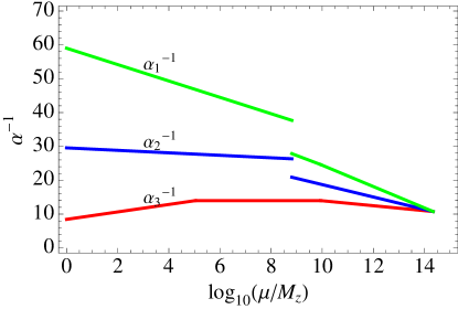
Figure 3: RG flows of the subgroups of $SU(5)_{F}$, with $T_{X}=10^{7}$ GeV, $T_{\chi}=3.8\times 10^{10}$ GeV, $T_{\rho}=7.9\times 10^{11}$ GeV, and $T_{GUT}=2\times 10^{16}$ GeV. The green, blue, and red lines correspond to the gauge couplings of $U(1)_{Y}\times SU(2)_{L}\times SU(3)_{c}$ below $T_{\chi}$ and $U(1)_{F}\times SU(2)_{F}\times SU(3)_{c}$ above $T_{\chi}$ respectively. The input parameters for the couplings are in Eq. (48).

III.2 soft SUSY breaking terms

We qualitatively evaluate the soft SUSY breaking terms in this scenario. According to the analysis in Sec. II.4, the gaugino masses at $\mu<T_{\chi}$ are written as

$$M_{2}(\mu) = -3\frac{\alpha_{2}(\mu)}{4\pi}\frac{F_{X}}{|\Delta v|},$$ (45)

$$M_{3}(\mu) = -(2-\xi)\frac{\alpha_{{3}}(\mu)}{4\pi}\frac{F_{X}}{|\Delta v|},$$ (46)

$$M_{1}(\mu) = -\left(\frac{37-2\xi}{5}\right)\frac{\alpha_{1}(\mu)}{4\pi}\frac{F_{X}}{|\Delta v|}.$$ (47)

Let us consider the case with $\xi=1$ and the gaugino masses at the EW scale. The gauge couplings at the EW scale are PDG

$$\alpha_{1}(M_{Z})\approx 0.01695,~{}\alpha_{2}(M_{Z})\approx 0.03382,~{}\alpha_{3}(M_{Z})\approx 0.1185,$$ (48)

so that we could derive the following mass relation:

$$\frac{M_{1}(M_{Z})}{M_{3}(M_{Z})}\approx 1.001,~{}\frac{M_{2}(M_{Z})}{M_{3}(M_{Z})}\approx 0.856.$$ (49)

The masses are almost degenerate, and this may be a specific feature of the gauge messenger model Dermisek ; Bae . If all intermediate scales are close to the GUT scale, the fine-tuning of $\mu$ term may be drastically reduced, as discussed in Ref. AKO3 . Fig. 2 tells us that the extra $SU(3)$-adjoint field reside in the low-scale, so that the condition for the small $\mu$-term would be modified. The one-loop running correction of $m^{2}_{H_{u}}$ with $T_{X}=10^{7}$ GeV from $T_{\chi}$ to $M_{Z}$ is estimated as

$$\Delta m^{2}_{H_{u}}\approx-0.276M_{3}(M_{Z})^{2}-0.047M_{2}(M_{Z})M_{3}(M_{Z})+0.221M_{2}(M_{Z})^{2}+\dots,$$ (50)

where the ellipsis denotes the terms including A-term and scalar masses and those are not important when they are comparable to the gluino mass. This leads that the condition to cancel the large contribution of gluino is $M_{2}/M_{3}(M_{Z})\approx 1.23$, which suggests the almost degenerate mass spectrum. However, we have a large A-term contribution to $\Delta m^{2}_{H_{u}}$ in our model, so that it may be difficult to avoid a certain fine-tuning even if the gaugino masses are degenerate.

According to Eqs. (42) and (41), the masses squared of superpartners and A-term are evaluated explicitly. Setting $T_{G}=T_{H_{c}}>T_{\rho}>T_{\chi}$ and $\xi=1$, stop masses at $T_{\chi}$ are given by

$$m_{Q}^{2}(T_{\chi}) \approx \left(8.83-6.67\frac{\alpha^{2}_{3}(T_{\rho})}{\alpha^{2}_{G}}-10.80\frac{\alpha^{2}_{F_{2}}(T_{\chi})}{\alpha^{2}_{G}}-0.33\frac{\alpha^{2}_{F_{1}}(T_{\chi})}{\alpha^{2}_{G}}\right)\Lambda^{2}_{SUSY},$$ (51)

$$m_{U}^{2}(T_{\chi}) \approx \left(8.60-6.67\frac{\alpha^{2}_{3}(T_{\rho})}{\alpha^{2}_{G}}-5.30\frac{\alpha^{2}_{F_{1}}(T_{\chi})}{\alpha^{2}_{G}}-0.01\frac{\alpha^{2}_{F_{1}}(T_{\rho})}{\alpha^{2}_{G}}\right)\Lambda^{2}_{SUSY}.$$ (52)

As we see, large stop masses are generated by the large second casimir $(c^{t}_{2}=18/5)$, but they might be driven to the tachyonic if $T_{\chi}$ and $T_{\rho}$ are close to the GUT scale. The SUSY scale $(\Lambda_{SUSY})$ from the gauge mediation is defined as

$$\Lambda_{SUSY}=\frac{\alpha_{G}}{(4\pi)}\frac{F_{X}}{|\Delta v|}\approx\frac{\alpha_{G}}{(4\pi)}\frac{M_{p}}{T_{G}}m_{3/2}.$$ (53)

$\alpha_{G}$ is of $O(0.1)$ when $T_{G}$ is around $10^{16}$ GeV, so that $\Lambda_{SUSY}$ might be compatible with $m_{3/2}$. If $T_{G}$ is smaller, the situation, $\Lambda_{SUSY}\gg m_{3/2}$, is achieved but suffers from the constraint from proton decay. The correction from the gravity mediation is naively estimated as $O(m_{3/2})$. It is almost the same order as the one from the gauge mediation in our model, and it may make it difficult to control flavors. In fact, the gauge-mediation contributions are typically at least $5$ times as large as the gravitino mass in our model, as we see in Table 4. In this case, we could expect the gravity-mediation effect is sub-dominant, and the SUSY scale is governed by the gauge-mediation. However, the gravity-mediation contribution should be $O(10^{-2})$ times suppressed, if it contributes to the sparticles masses squared flavor-universally Gabbiani:1996hi . In order to realize such a suppression and control flavor in the MSSM, we have to consider flavor symmetry or some dynamics above the GUT scale, as discussed in Refs. conformal . Indeed, explicit contributions on soft masses through the gravity mediation depend on the UV completion of our model. In this letter, one of our main motivations is to achieve $125$ GeV Higgs mass and realistic EW symmetry breaking, which may be independent of this issue about the constraint from flavor physics, so that we will discuss our SUSY mass spectrums assuming that the gauge-mediation is dominant. The underlying theory above the GUT scale will be studied in Ref. progress .

$A_{t}$, which is the trilinear coupling of stops ($\widetilde{t}$) as $y_{t}A_{t}\widetilde{t}_{L}H_{u}\widetilde{t}_{R}$ is given by

$$A_{t}(T_{\chi})\approx\left(22.57-8.00\frac{\alpha_{3}(T_{\rho})}{\alpha_{G}}-3.6\frac{\alpha_{F_{2}}(T_{\chi})}{\alpha_{G}}-0.98\frac{\alpha_{F_{1}}(T_{\chi})}{\alpha_{G}}+0.01\frac{\alpha_{F_{1}}(T_{\rho})}{\alpha_{G}}\right)\Lambda_{SUSY},$$ (54)

and the B-term, which is the bilinear coupling of two Higgs $\mu BH_{u}H_{d}$, is estimated as

$$B(T_{\chi})\approx\left(10.27-3.60\frac{\alpha_{F_{2}}(T_{\chi})}{\alpha_{G}}-0.68\frac{\alpha_{F_{1}}(T_{\chi})}{\alpha_{G}}+0.01\frac{\alpha_{F_{1}}(T_{\rho})}{\alpha_{G}}\right)\Lambda_{SUSY}.$$ (55)

As we see, the A-term and B-term might be large as $O(10)\Lambda_{SUSY}$. This may be good to achieve the EW symmetry breaking, but too large A-term makes the stop masses tachyonic because of the running correction such as

$$\Delta m^{2}_{U}(M_{Z})\approx-0.08A_{t}(T_{\chi})^{2}+1.54M_{3}(T_{\chi})^{2}-0.15A_{t}(T_{\chi})M_{3}(T_{\chi}).$$ (56)

In our model, the gluino mass $M_{3}$ is relatively small as wee see in Eq. (46), so $\Delta m^{2}_{U}(M_{Z})$ becomes easily negative and stop mass becomes tachyonic even if the positive $m^{2}_{U}$ is generated at the SUSY breaking scale $T_{\chi}$. In order to avoid the tachyonic stop masses, we add an extra contribution to the gluino mass, as we see below.

III.3 Shift of the gluino mass

We consider an extra term, which contributes to the gluino mass,

$$W=\frac{1}{\Lambda_{0}}Tr_{5}(\Phi W_{5}W_{5}).$$ (57)

There are several ways to introduce this term, such as gravity effect. Here, we simply assume that $N_{\rm extra}$ extra heavy $SU(5)$ vector-like pairs ($\psi,\overline{\psi}$) with the masses $\overline{\psi}(\Lambda_{0}+\lambda_{X}\Phi)\psi$ induce this term, integrating out them at the scale $\Lambda_{0}$. After the $SU(5)$ breaking, the gauge coupling would have the extra $v_{X}$ dependence as

$$\alpha^{-1}_{3}\to\alpha^{-1}_{3}-\frac{N_{\rm extra}}{4\pi}\ln\left(\frac{(|\Lambda_{0}+\lambda_{X}(v_{X}+F_{X}\theta^{2})|^{2})}{\Lambda^{2}}\right).$$ (58)

This additional coupling could shift the gluino mass as

$$M_{3}\to M_{3}-\frac{\alpha_{3}N_{eff}}{4\pi}\frac{F_{X}}{|\Delta v|},$$ (59)

where $N_{eff}$ may not be $N_{\rm extra}$ because of the scale difference between $\Lambda_{0}$ and the GUT scale. Including $N_{eff}$, the gluino mass becomes

$$M_{3}(\mu)=-(1-N_{eff})\frac{\alpha_{{3}}(\mu)}{4\pi}\frac{F_{X}}{|\Delta v|},$$ (60)

so $N_{eff}$ should be bigger than $2$ in order to shift $M_{3}$. In fact, we discuss large $N_{eff}$ cases and find that $N_{eff}$ enables us to evade the negative squared masses and achieve the large SM Higgs mass.

III.4 Consistency with the Higgs mass and the EW symmetry breaking

One issue in supersymmetric models is how to realize the $\mu$ and $B$ terms which are consistent with the EW scale. Especially, $\mu$ relates to the lightest Higgs mass, because of the upper bound in MSSM, so that the recent Higgs discovery with the mass $125$ GeV may impose unnatural SUSY scenarios on us. In fact, $125$ GeV Higgs mass may require $\Lambda_{SUSY}\gtrsim O(10)$ TeV in the simple scenarios as discussed in Ref. Higgs1 . $O(10)$-TeV SUSY scale would require $0.01\%$ fine-tuning against $\mu$ without any cancellation in $m^{2}_{H_{u}}$. As pointed out in Refs. Higgs2 ; Higgs3 , it is known that a special relation between $A_{t}$ and squark mass relaxes the fine-tuning, maximizing the loop corrections in the Higgs mass in the MSSM. This relation is so-called “maximal mixing” and described as $X_{t}/m_{stop}=\sqrt{6}$, where $X_{t}=A_{t}-\mu/\tan\beta$ and $m_{stop}^{2}=\sqrt{m_{Q}^{2}m_{U}^{2}}$ are defined. If this relation is satisfied, the $125$ GeV Higgs mass could be achieved even if the stop is light. We can see our prediction on $X_{t}$ and the upper bound on the Higgs mass in the case with $0\leq N_{eff}\leq 6$ (light blue), $6\leq N_{eff}\leq 8$ (light red) in Fig. 4. On the all regions, all masses squared of the superpartners are positive and $(T_{G},T_{X})$ are fixed at $(2\times 10^{16}{\rm GeV},$ $10^{7}{\rm GeV})$. We find that our A-term is too large to realize $X_{t}/m_{stop}=\sqrt{6}$, but the maximal mixing could be achieved, if we allow large $N_{eff}$, and enhance the Higgs mass, even if $m_{stop}$ is around $1$ TeV.

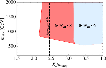
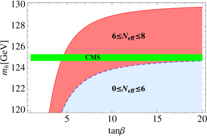
Figure 4: $X_{t}/m_{stop}$ vs. $m_{stop}$ and $\tan\beta$ vs. the lightest Higgs mass in the case with $(T_{\rm GUT},T_{X})=(2\times 10^{16}{\rm GeV},$ $10^{7}{\rm GeV})$ and $0\leq N_{eff}\leq 6$ (light blue), $6\leq N_{eff}\leq 8$ (light red). The dashed line corresponds to $X_{t}/m_{stop}=\sqrt{6}$. In the right figure, $m_{h}$ is calculated at the two-loop level using $m_{t}=172.9$ GeV, and $m_{stop}$ is lighter than $2$ TeV. The green band is the CMS result on Higgs mass from $h\to\gamma\gamma$, $ZZ$ channels Higgs-CMS .

On the other hand, we notice that there is no special cancellation in $m^{2}_{H_{u}}$ and $m^{2}_{H_{d}}$, as we see in Fig. 5. Large $m_{stop}$ corresponds to large $\mu$, so that $1$-TeV squark mass requires $1\%$ fine-tuning against $\mu$. The right figure in Fig. 5 shows that small $\tan\beta$ is consistent with the EW symmetry breaking. $B_{\rm EW}$ is the value to realize the EW symmetry breaking,

$$B_{\rm EW}\equiv-\frac{1}{2\mu}\{(m^{2}_{H_{d}}-m^{2}_{H_{u}})\tan 2\beta+M_{Z}^{2}\sin 2\beta\},$$ (61)

and $B$ is our prediction via the gauge mediation. It seems that $2\lesssim\tan\beta\lesssim 6$ is necessary to achieve $125$ GeV Higgs mass. The $\tan\beta$ region may be inconsistent with the one required by $125$ GeV Higgs ($\tan\beta\gtrsim 4$) with $m_{stop}\leq 2$ TeV. Table 4 in Appendix B shows the parameter sets in our model, which satisfy $m_{h}\approx 125$ GeV and $|B_{\rm EW}/B|\approx 1$. There, $m_{stop}$ and $|\mu|$ are around $3$ TeV, and $O(0.1)$ % fine-tuning is required against $\mu$ term.

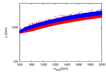
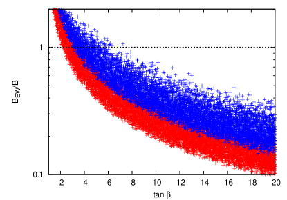
Figure 5: $m_{stop}$ vs. $\mu$ and $\tan\beta$ vs. B-term in the case with $(T_{\rm GUT},T_{X})=(2\times 10^{16}{\rm GeV},$ $10^{7}{\rm GeV})$ and $0\leq N_{eff}\leq$ (blue), $6\leq N_{eff}\leq 8$ (red). In the right figure, $m_{stop}$ is lighter than $2$ TeV. The dashed line is consistent with the condition for the EW symmetry breaking.

IV $SU(5)_{F}\times SU(3)\times U(1)_{\phi}$ gauge theory: $(N_{F},N)=(5,3)$

Our symmetry breaking model could be embed into other type GUT model. One simple example would be the $SU(5)_{F}\times SU(3)\times U(1)_{\phi}$ gauge symmetric model, and we could consider the same setup as in the $SU(5)_{F}\times SU(2)\times U(1)_{\phi}$ gauge theory. The visible sector is given by Eq. (43). However, the modification of the Higgs sector may be required because $\lambda\overline{H}\Phi H$ term gives the very large B-term, $\lambda F_{X}H_{u}H_{d}$. There may be a solution to realize the EW symmetry breaking, but the serious fine-tuning may be required. Here, we consider another solution to shift the colored Higgs mass which maybe favor high-scale SUSY.

We introduce $SU(3)$ vector-like fields $(H_{3},\overline{H}_{3})$ and assign $Z_{3}$ symmetry to the fields as in Table 3. $Z_{3}$ symmetry is broken by the VEV of $S$. The superpotential for the Higgs sector is given by

$$W_{H}=\lambda_{S}S\overline{H}H+\lambda_{\phi}\overline{H}\overline{H}_{3}\phi+\lambda_{\widetilde{\phi}}\widetilde{\phi}H_{3}H+\frac{\lambda_{3}}{3}S^{3}.$$ (62)

	$\overline{\bf 5}_{i}$	${\bf 10}_{i}$	$H$	$\overline{H}$	$H_{3}$	$\overline{H}_{3}$	$S$	$\phi$	$\widetilde{\phi}$	$\Phi$
$SU(5)_{F}$	$\overline{\bf 5}$	10	5	$\overline{{\bf 5}}$	1	1	1	5	$\overline{{\bf 5}}$	adj5+1
$SU(3)$	1	1	1	1	3	$\overline{\bf 3}$	1	3	$\overline{\bf 3}$	1
$U(1)_{\phi}$	0	0	0	0	$Q_{\phi}$	$-Q_{\phi}$	0	$Q_{\phi}$	$-Q_{\phi}$	0
$Z_{3}$	${\bf\omega}$	${\bf\omega}$	${\bf\omega}$	${\bf\omega}$	${\bf\omega}^{2}$	${\bf\omega}^{2}$	${\bf\omega}$	1	1	1

Table 3: Chiral superfields in $SU(5)_{F}\times SU(3)\times U(1)$ gauge theory

After the GUT symmetry breaking, $(H,\overline{H})$ are decomposed as $((H_{u},H^{\prime}_{3}),(H_{d},\overline{H}^{\prime}_{3}))$ and the mass terms for $(H_{3},\overline{H}^{\prime}_{3})$ and $(H^{\prime}_{3},\overline{H}_{3})$ pairs appear as

$$W^{eff}_{H}=\lambda_{\phi}v_{\chi}\overline{H}^{\prime}_{3}\overline{H}_{3}+\lambda_{\widetilde{\phi}}v_{\chi}H_{3}H^{\prime}_{3}.$$ (63)

$H_{u}$ and $H_{d}$ correspond to the Higgs $SU(2)_{L}$ doublets in MSSM, and they could get the supersymmetric mass term according to the nonzero VEV of $S$. In Refs. productGUT , we can see not only the $SU(5)_{F}\times SU(2)\times U(1)_{\phi}$-type but also this type of product-GUT.

In order to avoid the bound from the proton decay caused by the five dimensional operators, $v_{\chi}$ should be large as

$$v_{\chi}\gtrsim 10^{16}{\rm GeV}\times\left(\frac{1{\rm TeV}}{\Lambda_{\rm SUSY}}\right).$$ (64)

$F_{X}$ is given by $-hv^{2}_{\chi}$, so that very tiny $h$ is necessary to achieve the low-scale SUSY. When $v_{\chi}\approx 10^{16}$ GeV and $\Lambda_{\rm SUSY}=1$ TeV are set, $h$ should be around $O(10^{-10})$, because of

$$h=\frac{4\pi}{\alpha_{G}}\frac{\Delta v}{v^{2}_{\chi}}\Lambda_{\rm SUSY}\approx 10^{-10}\times\left(\frac{10^{16}\rm GeV}{v_{\chi}}\right)^{2}\left(\frac{\Lambda_{\rm SUSY}}{1\rm TeV}\right)\lesssim 10^{-10}\times\left(\frac{\Lambda_{\rm SUSY}}{1\rm TeV}\right)^{3}.$$ (65)

We conclude that high-scale SUSY is favored to avoid such an extremely small $h$.

We can consider the applications of our symmetry breaking models to the other BSMs, such as

• $SU(3)_{c}\times SU(2)_{L}\times SU(2)_{R}\times U(1)_{B-L}\rightarrow SU(3)_{c}\times SU(2)_{L}\times U(1)_{Y},$

• $SU(4)\times SU(2)_{L}\times U(1)\rightarrow SU(3)_{c}\times SU(2)_{L}\times U(1)_{Y}.$

We would study such patterns elsewhere progress . In these models, all of chiral superfields appear as adjoint representations and bi-fundamental representations. Such models can be constructed in D-brane models, e.g. intersecting/magnetized D-brane models (see for a review Blumenhagen:2006ci ; Ibanez and references therein). Thus, the above models are interesting from the viewpoint of superstring theory.

V Summary

The MSSM is one of the attractive BSMs to solve the hierarchy problem in the SM and it may be expected to be found near future. One big issue in the MSSM is how to control the SUSY breaking parameters, so that many ideas and works on spontaneous SUSY breaking and mediation mechanisms of the SUSY breaking effects have been discussed so far. In this paper, we proposed an explicit and simple supersymmetric model, where the spontaneous SUSY breaking and GUT breaking are achieved by the same sector. The origin of the hyper-charge assignment in the MSSM is also explained by the analogy with the Georgi-Glashow $SU(5)$ GUT. The SM-charged particles are also introduced by the breaking sector, so that we could also predict the soft SUSY breaking terms via the gauge mediation with the gauge and chiral messenger superfields. The crucial role of the gauge-messenger mediation is to induce large A-terms and B-terms at the one-loop level. We investigated the scenario with light superpartners that such a large A-term realizes the maximal mixing and shift the lightest Higgs mass. In fact, we have to introduce additional contribution to the gluino mass, but $125$ GeV Higgs mass could be achieved, even if stop is light. $m_{stop}$ should be as light as possible to relax the fine-tuning of $\mu$ parameter. On the other hand, the one-loop B-term could be also consistent with the EW symmetry breaking, if $\tan\beta$ is within $2\lesssim\tan\beta\lesssim 6$. Such small $\tan\beta$ may require large stop mass, as we see in Figs. 4 and 5. In fact, we see that about $3$ TeV $m_{stop}$ can achieve $125$ GeV Higgs mass and the EW symmetry breaking in Table 4.

Our light SUSY particles are wino, bino, and gravitino, and the mass difference is not so big. The lightest particle is bino, and wino is heavier than bino. The mass difference is $O(0.1)\times m_{3/2}$ GeV. This might be one specific feature of the gauge messenger scenario in $SU(5)$ GUT, as discussed in Ref. Bae .

Appendix A mass spectrums of the particles in the symmetry breaking sector

We investigate the mass matrices for the remnant fields in the symmetry breaking sector. First, let us discuss $(Z,\widetilde{Z})$ and $(\rho,\widetilde{\rho})$ components. We define $Z_{\pm}$ and $\rho_{\pm}$ as

$$Z_{\pm}=\frac{\widetilde{Z}\pm Z^{\dagger}}{\sqrt{2}},~{}\rho_{\pm}=\frac{\rho\pm\widetilde{\rho}^{\dagger}}{\sqrt{2}}.$$ (66)

The fermion masses are given by

$${\cal L}_{f} = -\begin{pmatrix}\overline{\lambda_{-}}&\overline{Z_{+}}&\overline{\rho_{+}}\end{pmatrix}M^{f}_{+}\begin{pmatrix}\lambda_{-}\\ Z_{+}\\ \rho_{+}\end{pmatrix}-\begin{pmatrix}\overline{\lambda_{+}}&\overline{Z_{-}}&\overline{\rho_{-}}\end{pmatrix}M^{f}_{-}\begin{pmatrix}\lambda_{+}\\ Z_{-}\\ \rho_{-}\end{pmatrix},$$ (67)

where the mass matrices $(M^{f}_{\pm})$ are

$$M^{f}_{+}=\begin{pmatrix}0&-g\Delta v&gv_{\chi}\\ -g\Delta v&0&-hv_{\chi}\\ gv_{\chi}&-hv_{\chi}&-h\Delta v\end{pmatrix},~{}M^{f}_{-}=\begin{pmatrix}0&-g\Delta v&gv_{\chi}\\ -g\Delta v&0&hv_{\chi}\\ gv_{\chi}&hv_{\chi}&h\Delta v\end{pmatrix},$$ (68)

and $\lambda_{\pm}$ are the linear combinations of the gauginos $(X_{(+)})$ which are the suparpartners of $X_{\mu}$,

$$\lambda_{\pm}=\frac{X_{+}\pm\overline{X}}{\sqrt{2}}.$$ (69)

The masses for the bosonic superpartners are

$${\cal L}_{B} = -\begin{pmatrix}Z^{\dagger}_{+}&\rho^{\dagger}_{+}\end{pmatrix}M^{2}_{+}\begin{pmatrix}Z_{+}\\ \rho_{+}\end{pmatrix}-\begin{pmatrix}Z^{\dagger}_{-}&\rho^{\dagger}_{-}\end{pmatrix}M^{2}_{-}\begin{pmatrix}Z_{-}\\ \rho_{-}\end{pmatrix},$$ (70)

where the mass matrices $(M^{2}_{\pm})$ are given by

$$M^{2}_{+} = \begin{pmatrix}h^{2}v_{\chi}^{2}&-h^{2}v_{\chi}\Delta v\\ -h^{2}v_{\chi}\Delta v&h^{2}(v_{\chi}^{2}+\Delta v^{2})+F_{X}\end{pmatrix},$$ (71)

$$M^{2}_{-} = \begin{pmatrix}h^{2}v_{\chi}^{2}+g^{2}\Delta v^{2}&-(h^{2}+g^{2})\Delta vv_{\chi}\\ -(h^{2}+g^{2})\Delta vv_{\chi}&h^{2}(v_{\chi}^{2}+\Delta v^{2})+g^{2}v_{\chi}^{2}-F_{X}\end{pmatrix}.$$ (72)

The F-term $F_{X}$ is $F_{X}=-h^{2}v^{2}_{\chi},$ so that $M^{2}_{+}$ includes the Goldstone mode.

The fermion masses for the other particles are also generated by the VEVs:

$${\cal L}_{Y} = -\frac{1}{2}\begin{pmatrix}\widetilde{W}^{A}&Y^{A}\end{pmatrix}M_{Y}\begin{pmatrix}\chi^{A}\\ \widetilde{\chi}^{A}\end{pmatrix}-\frac{1}{2}\begin{pmatrix}\chi^{A}&\widetilde{\chi}^{A}\end{pmatrix}M^{T}_{Y}\begin{pmatrix}\widetilde{W}^{A}\\ Y^{A}\end{pmatrix}+h.c.,$$ (73)

where $\widetilde{W}$ is the superpartner of $W^{\prime}$ and $M_{Y}$ are defined as

$$M_{Y} = \left(\begin{array}[]{cc}-\frac{1}{\sqrt{2}}M_{W^{\prime}}&\frac{1}{\sqrt{2}}M_{W^{\prime}}\\ -hv_{\chi}&-hv_{\chi}\\ \end{array}\right).$$ (76)

The eigenvalues are $M_{W^{\prime}},~{}M_{W^{\prime}},~{}\sqrt{2}hv_{\chi},~{}\sqrt{2}hv_{\chi}$ and the bosonic masses are given by the same mass spectrum. The imaginary part of $\chi-\widetilde{\chi}$ corresponds to the Goldstone boson, and the real part has the mass, $M_{W^{\prime}}$, according to the D-term. The other masses, $\sqrt{2}hv_{\chi}$, correspond to the ones of $\chi+\widetilde{\chi}$ and $Y$.

The singlet components $(Y_{0},\chi_{0},\widetilde{\chi}_{0})$ of $\hat{Y}$ and $(\hat{\chi},\hat{\widetilde{\chi}})$ also get masses, according to the nonzero $v_{\chi}$. The fermionic mass matrix is

$${\cal L}_{Y_{0}} = -\frac{1}{2}\begin{pmatrix}\widetilde{Z^{\prime}}&Y_{0}\end{pmatrix}M_{Y_{0}}\begin{pmatrix}\chi_{0}\\ \widetilde{\chi_{0}}\end{pmatrix}-\frac{1}{2}\begin{pmatrix}\chi_{0}&\widetilde{\chi_{0}}\end{pmatrix}M^{T}_{Y_{0}}\begin{pmatrix}\widetilde{Z^{\prime}}\\ Y_{0}\end{pmatrix}+h.c.,$$ (77)

where $M_{Y_{0}}$ are defined as

$$M_{Y_{0}} = \left(\begin{array}[]{cc}-\frac{1}{\sqrt{2}}M_{Z^{\prime}}&\frac{1}{\sqrt{2}}M_{Z^{\prime}}\\ -hv_{\chi}&-hv_{\chi}\\ \end{array}\right).$$ (80)

The mass spectrums are given, relplacing $M_{W^{\prime}}$ with $M_{Z^{\prime}}$.

Appendix B Concrete parameter set

The parameter sets which predict $m_{h}\approx 125$ GeV are in Table 4. The Higgs mass is calculated by FeynHiggs Higgs3 ; FeynHiggs . $m_{\widetilde{t}_{1,2}}$ are the stop masses in the mass eigenstate. $m^{2}_{\widetilde{Q}_{L}}$, $m^{2}_{\widetilde{d}_{R}}$, $m^{2}_{\widetilde{l}_{L}}$ and $m^{2}_{\widetilde{e}_{R}}$ are the soft SUSY breaking terms of the squarks $(\widetilde{Q}_{L},\widetilde{d}_{R})$ and sleptons $(\widetilde{l}_{L},\widetilde{e}_{R})$.

	$N_{eff}=6$	$N_{eff}=6$	$N_{eff}=6.97$	$N_{eff}=7.83$
$m_{3/2}$	$588.84$ GeV	$741.31$ GeV	$495.79$ GeV	$245.02$ GeV
$T_{\rho}$	$2.39\times 10^{11}$ GeV	$5.76\times 10^{12}$ GeV	$5.66\times 10^{12}$ GeV	$2.74\times 10^{10}$ GeV
$T_{X}$	$1.00\times 10^{7}$ GeV	$1.00\times 10^{7}$ GeV	$1.00\times 10^{7}$ GeV	$1.00\times 10^{7}$ GeV
$\tan\beta$	$3.69$	$3.93$	$3.43$	$4.04$
$m_{h}$	$126.20$ GeV	$125.89$ GeV	$124.65$ GeV	$124.03$ GeV
$m_{stop}$	$3.05$ TeV	$3.61$ TeV	$2.93$ TeV	$1.90$ TeV
$X_{t}$	$3.43\times$ $m_{stop}$	$3.41\times$ $m_{stop}$	$2.98\times$ $m_{stop}$	$2.39\times$ $m_{stop}$
$|\mu|$	$3.72$ TeV	$4.38$ TeV	$3.27$ TeV	$1.93$ TeV
$|B|$	$4.21$ TeV	$4.72$ TeV	$3.22$ TeV	$1.97$ TeV
$|B_{\rm{EW}}/B|$	$0.92$	$1.00$	$0.91$	$0.5$
$|M_{3}|$	$5.73\times m_{3/2}$	$5.73\times m_{3/2}$	$6.85\times m_{3/2}$	$7.83\times m_{3/2}$
$|M_{2}|$	$0.98\times m_{3/2}$	$0.98\times m_{3/2}$	$0.98\times m_{3/2}$	$0.98\times m_{3/2}$
$|M_{1}|$	$0.75\times m_{3/2}$	$0.75\times m_{3/2}$	$0.69\times m_{3/2}$	$0.64\times m_{3/2}$
$m_{\widetilde{t}_{1}}$	$3.52$ TeV	$4.12$ TeV	$3.31$ TeV	$2.15$ TeV
$m_{\widetilde{t}_{2}}$	$2.62$ TeV	$3.17$ TeV	$2.57$ TeV	$1.65$ TeV
$m^{2}_{\widetilde{Q}_{L}}$	$11.72$ TeV2	$16.56$ TeV2	$10.36$ TeV2	$4.24$ TeV2
$m^{2}_{\widetilde{d}_{R}}$	$15.97$ TeV2	$22.52$ TeV2	$13.60$ TeV2	$5.40$ TeV2
$m^{2}_{\widetilde{l}_{L}}$	$0.78$ TeV2	$0.93$ TeV2	$0.44$ TeV2	$0.18$ TeV2
$m^{2}_{\widetilde{e}_{R}}$	$1.42$ TeV2	$1.75$ TeV2	$0.81$ TeV2	$0.31$ TeV2

Table 4: SUSY mass spectrums and parameters with $\Lambda_{GUT}=2\times 10^{16}$ GeV. Higgs mass is calculated by FeynHiggs Higgs3 ; FeynHiggs .

References

- (1) S. Chatrchyan et al. [CMS Collaboration], Phys. Lett. B 716, 30 (2012) [arXiv:1207.7235 [hep-ex]]; G. Aad et al. [ATLAS Collaboration], Phys. Lett. B 716, 1 (2012) [arXiv:1207.7214 [hep-ex]].
- (2) K.A. Olive et al. (Particle Data Group), Chin. Phys. C, 38, 090001 (2014).
- (3) G. F. Giudice and A. Strumia, Nucl. Phys. B 858, 63 (2012) [arXiv:1108.6077 [hep-ph]]; G. Degrassi, S. Di Vita, J. Elias-Miro, J. R. Espinosa, G. F. Giudice, G. Isidori and A. Strumia, JHEP 1208, 098 (2012) [arXiv:1205.6497 [hep-ph]].
- (4) T. Hirayama, N. Ishimura and N. Maekawa, Prog. Theor. Phys. 101, 1343 (1999) [hep-ph/9805457]; K. Agashe, Phys. Lett. B 444, 61 (1998) [hep-ph/9809421]; K. Agashe, Nucl. Phys. B 588, 39 (2000) [hep-ph/0003236].
- (5) B. Bajc and G. Senjanovic, Phys. Lett. B 648, 365 (2007) [hep-ph/0611308]; B. Bajc and A. Melfo, JHEP 0804, 062 (2008) [arXiv:0801.4349 [hep-ph]]; B. Bajc, S. Lavignac and T. Mede, JHEP 1207, 185 (2012) [arXiv:1202.2845 [hep-ph]].
- (6) N. Arkani-Hamed, J. March-Russell and H. Murayama, Nucl. Phys. B 509, 3 (1998) [hep-ph/9701286]; E. Poppitz and S. P. Trivedi, Phys. Rev. D 55, 5508 (1997) [hep-ph/9609529]; N. Haba, N. Maru and T. Matsuoka, Phys. Rev. D 56, 4207 (1997) [hep-ph/9703250]; H. Murayama, Phys. Rev. Lett. 79, 18 (1997) [hep-ph/9705271]; M. A. Luty and J. Terning, Phys. Rev. D 57, 6799 (1998) [hep-ph/9709306]; K. Agashe, Phys. Lett. B 435, 83 (1998) [hep-ph/9804450]; R. Kitano, H. Ooguri and Y. Ookouchi, Phys. Rev. D 75, 045022 (2007) [hep-ph/0612139]; H. Murayama and Y. Nomura, Phys. Rev. Lett. 98, 151803 (2007) [hep-ph/0612186]; C. Csaki, Y. Shirman and J. Terning, JHEP 0705, 099 (2007) [hep-ph/0612241]; N. Haba and N. Maru, Phys. Rev. D 76, 115019 (2007) [arXiv:0709.2945 [hep-ph]]; S. A. Abel, C. Durnford, J. Jaeckel and V. V. Khoze, JHEP 0802, 074 (2008) [arXiv:0712.1812 [hep-ph]].
- (7) K. Intriligator, N. Seiberg and D. Shih, JHEP 0604, 021 (2006) [arXiv:hep-th/0602239].
- (8) R. Dermisek, H. D. Kim and I. W. Kim, JHEP 0610, 001 (2006) [hep-ph/0607169].
- (9) L. Matos, JHEP 1012, 042 (2010) [arXiv:1007.3616 [hep-ph]].
- (10) H. Abe, T. Kobayashi and Y. Omura, Phys. Rev. D 77, 065001 (2008) [arXiv:0712.2519 [hep-ph]].
- (11) H. Abe, T. Kobayashi and Y. Omura, JHEP 0711, 044 (2007) [arXiv:0708.3148 [hep-th]].
- (12) H. Abe, T. Higaki, T. Kobayashi and Y. Omura, Phys. Rev. D 75, 025019 (2007) [hep-th/0611024].
- (13) G. F. Giudice and R. Rattazzi, Nucl. Phys. B 511, 25 (1998) [hep-ph/9706540].
- (14) K. Intriligator and M. Sudano, JHEP 1006, 047 (2010) [arXiv:1001.5443 [hep-ph]].
- (15) J. Hisano, H. Murayama and T. Goto, Phys. Rev. D 49, 1446 (1994).
- (16) T. Goto and T. Nihei, Phys. Rev. D 59, 115009 (1999) [hep-ph/9808255]; H. Murayama and A. Pierce, Phys. Rev. D 65, 055009 (2002) [hep-ph/0108104].
- (17) K. J. Bae, R. Dermisek, H. D. Kim and I. W. Kim, JCAP 0708, 014 (2007) [hep-ph/0702041 [HEP-PH]].
- (18) K. Choi, K. S. Jeong, T. Kobayashi and K. i. Okumura, Phys. Lett. B 633, 355 (2006) [hep-ph/0508029].
- (19) H. Abe, T. Kobayashi and Y. Omura, Phys. Rev. D 76, 015002 (2007) [hep-ph/0703044].
- (20) F. Gabbiani, E. Gabrielli, A. Masiero and L. Silvestrini, Nucl. Phys. B 477, 321 (1996) [hep-ph/9604387].
- (21) M. A. Luty and R. Sundrum, Phys. Rev. D 65, 066004 (2002) [hep-th/0105137]; M. Luty and R. Sundrum, Phys. Rev. D 67, 045007 (2003) [hep-th/0111231]; R. Sundrum, Phys. Rev. D 71, 085003 (2005) [hep-th/0406012]; M. Ibe, K.-I. Izawa, Y. Nakayama, Y. Shinbara and T. Yanagida, Phys. Rev. D 73, 015004 (2006) [hep-ph/0506023]; M. Ibe, K.-I. Izawa, Y. Nakayama, Y. Shinbara and T. Yanagida, Phys. Rev. D 73, 035012 (2006) [hep-ph/0509229]; M. Schmaltz and R. Sundrum, JHEP 0611, 011 (2006) [hep-th/0608051]; H. Murayama, Y. Nomura and D. Poland, Phys. Rev. D 77, 015005 (2008) [arXiv:0709.0775 [hep-ph]].
- (22) M. S. Carena, M. Quiros and C. E. M. Wagner, Nucl. Phys. B 461, 407 (1996) [hep-ph/9508343].
- (23) T. Hahn, S. Heinemeyer, W. Hollik, H. Rzehak and G. Weiglein, Phys. Rev. Lett. 112, 141801 (2014) [arXiv:1312.4937 [hep-ph]].
- (24) CMS Collaboration, CMS-PAS-HIG-14-009, CERN, Geneva Switzerland (2014).
- (25) T. Yanagida, Phys. Lett. B 344, 211 (1995) [hep-ph/9409329]; J. Hisano and T. Yanagida, Mod. Phys. Lett. A 10, 3097 (1995) [hep-ph/9510277]; K. I. Izawa and T. Yanagida, Prog. Theor. Phys. 97, 913 (1997) [hep-ph/9703350]; T. Watari and T. Yanagida, hep-ph/0208107; M. Ibe and T. Watari, Phys. Rev. D 67, 114021 (2003) [hep-ph/0303123]; T. Watari and T. Yanagida, Phys. Rev. D 70, 036009 (2004) [hep-ph/0402160]; F. Brümmer, M. Ibe and T. T. Yanagida, Phys. Lett. B 726, 364 (2013) [arXiv:1303.1622 [hep-ph]].
- (26) Work in progress.
- (27) R. Blumenhagen, B. Kors, D. Lust and S. Stieberger, Phys. Rept. 445, 1 (2007) [hep-th/0610327].
- (28) L. E. Ibanez and A. M. Uranga, “String theory and particle physics: An introduction to string phenomenology,” Cambridge University Press (2012).
- (29) S. Heinemeyer, W. Hollik and G. Weiglein, Comput. Phys. Commun. 124, 76 (2000) [hep-ph/9812320]; S. Heinemeyer, W. Hollik and G. Weiglein, Eur. Phys. J. C 9, 343 (1999) [hep-ph/9812472]; G. Degrassi, S. Heinemeyer, W. Hollik, P. Slavich and G. Weiglein, Eur. Phys. J. C 28, 133 (2003) [hep-ph/0212020]; M. Frank, T. Hahn, S. Heinemeyer, W. Hollik, H. Rzehak and G. Weiglein, JHEP 0702, 047 (2007) [hep-ph/0611326].