Test of Independence for High-dimensional Random Vectors Based on Block Correlation Matrices

In this paper, we are concerned with the independence test for $k$ high-dimensional sub-vectors of a normal vector, with fixed positive integer $k$. A natural high-dimensional extension of the classical sample correlation matrix, namely block correlation matrix, is raised for this purpose. We then construct the so-called Schott type statistic as our test statistic, which turns out to be a particular linear spectral statistic of the block correlation matrix. Interestingly, the limiting behavior of the Schott type statistic can be figured out with the aid of the Free Probability Theory and the Random Matrix Theory. Specifically, we will bring the so-called real second order freeness for Haar distributed orthogonal matrices, derived in Mingo and Popa (2013), into the framework of this high-dimensional testing problem. Our test does not require the sample size to be larger than the total or any partial sum of the dimensions of the $k$ sub-vectors. Simulated results show the effect of the Schott type statistic, in contrast to those of the statistics proposed in Jiang and Yang (2013) and Jiang, Bai and Zheng (2013), is satisfactory. Real data analysis is also used to illustrate our method.

Keywords: Block correlation matrix; Independence test; High dimensional data; Schott type statistic; Second order freeness; Haar distributed orthogonal matrices; Central limit theorem; Random matrices.

1 Introduction

Test of independence for random variables is a very classical hypothesis testing problem, which dates back to the seminal work by Pearson (1900), followed by a huge literature regarding this topic and its variants. One frequently recurring variant is the test of independence for $k$ random vectors, where $k\geq 2$ is an integer. Comprehensive overview and detailed references on this problem can be found in most of the textbooks on multivariate statistical analysis. For instance, here we recommend the masterpieces by Muirhead (1982) and by Anderson (2003) for more details, in the low-dimensional case. However, due to the increasing demand in the analysis of big data springing up in various fields nowadays, such as genomics, signal processing, microarray, proteomics and finance, the investigation on a high-dimensional extension of this testing problem is much needed, which motivates us to propose a feasible way for it in this work.

Let us take a review more specifically on some representative existing results in the literature, after necessary notation is introduced. For simplicity, henceforth, we will use the notation $\llbracket m\rrbracket$ to denote the set $\{1,2,\ldots,m\}$ for any positive integer $m$. Assume that $\mathbf{x}=(\mathbf{x}_{1}^{\prime},\ldots,\mathbf{x}_{k}^{\prime})^{\prime}$ is a $p$-dimensional normal vector, in which $\mathbf{x}_{i}$ possesses dimension $p_{i}$ for $i\in\llbracket k\rrbracket$, such that $p_{1}+\cdots+p_{k}=p$. Denote by $\bm{\mu}_{i}$ the mean vector of the $i$th sub-vector $\mathbf{x}_{i}$ and by $\Sigma_{ij}$ the cross covariance matrix of $\mathbf{x}_{i}$ and $\mathbf{x}_{j}$ for all $i,j\in\llbracket k\rrbracket$. Then $\bm{\mu}:=(\bm{\mu}_{1}^{\prime},\ldots,\bm{\mu}_{k}^{\prime})^{\prime}$ and $\Sigma:=(\Sigma_{ij})_{k,k}$ are the mean vector and covariance matrix of $\mathbf{x}$ respectively. In this work, we consider the following hypothesis testing

$$(\mathbf{T1})\hskip 43.05542pt\mathbf{H}_{0}:\Sigma_{ij}=0,\quad i\neq j\hskip 21.52771pt\text{v.s.}\hskip 21.52771pt\mathbf{H}_{1}:\text{ not }\mathbf{H}_{0}.$$

To this end, we draw $n$ observations of $\mathbf{x}$, namely $\mathbf{x}(1),\ldots,\mathbf{x}(n)$. In addition, the $i$th sub-vector of $\mathbf{x}(j)$ will be denoted by $\mathbf{x}_{i}(j)$ for all $i\in\llbracket k\rrbracket$ and $j\in\llbracket n\rrbracket$. Hence, $\mathbf{x}_{i}(j),j\in\llbracket n\rrbracket$ are $n$ independent observations of $\mathbf{x}_{i}$. Conventionally, the corresponding sample means will be written as $\bar{\mathbf{x}}=n^{-1}\sum_{j=1}^{n}\mathbf{x}(j)$ and $\bar{\mathbf{x}}_{i}=n^{-1}\sum_{j=1}^{n}\mathbf{x}_{i}(j)$. With the observations at hand, we can construct the sample covariance matrix as usual. Set

$$\mathbf{X}:=[\mathbf{x}(1)-\bar{\mathbf{x}},\cdots,\mathbf{x}(n)-\bar{\mathbf{x}}],\quad\mathbf{X}_{i}:=[\mathbf{x}_{i}(1)-\bar{\mathbf{x}}_{i},\cdots,\mathbf{x}_{i}(n)-\bar{\mathbf{x}}_{i}],\quad i\in\llbracket k\rrbracket.$$ (1)

The sample covariance matrix of $\mathbf{x}$ and the cross sample covariance matrix of $\mathbf{x}_{m}$ and $\mathbf{x}_{\ell}$ will be denoted by $\hat{\Sigma}$ and $\hat{\Sigma}_{m\ell}$ respectively, to wit,

$$\hat{\Sigma}:=\frac{1}{n-1}\mathbf{X}\mathbf{X}^{\prime},\hskip 34.44434pt\hat{\Sigma}_{m\ell}:=\frac{1}{n-1}\mathbf{X}_{m}\mathbf{X}_{\ell}^{\prime}.$$

In the classical large $n$ and fixed $p$ case, the likelihood ratio statistic $\Lambda_{n}:=W_{n}^{n/2}$ with

$$W_{n}:=\frac{|\hat{\Sigma}|}{\prod_{i=1}^{k}|\hat{\Sigma}_{ii}|}$$

is a favorable one aiming at the testing problem (T1). A celebrated limiting law on $\Lambda_{n}$ under $\mathbf{H}_{0}$ is

$$-2\kappa\log\Lambda_{n}\Longrightarrow\chi_{\rho}^{2},\quad\text{as }n\to\infty$$ (2)

where

$$\kappa=1-\frac{2(p^{3}-\sum_{i=1}^{k}p_{i}^{3})+9(p^{2}-\sum_{i=1}^{k}p_{i}^{2})}{6n(p^{2}-\sum_{i=1}^{k}p_{i}^{2})},\quad\rho=\frac{1}{2}(p^{2}-\sum_{i=1}^{k}p_{i}^{2}).$$

One can refer to Wilks (1935) or Theorem 11.2.5 of Muirhead (1982), for instance. The left hand side of (2) is known as the Wilks statistic.

Now, we turn to the high-dimensional setting of interest. A commonly used assumption on dimensionality and sample size in the Random Matrix Theory (RMT) is that $p$ is proportionally large as $n$, i.e.

$$p:=p(n),\quad\frac{p}{n}\to y\in(0,\infty),\text{ as }n\to\infty.$$

To employ the existing RMT apparatus in the sequel, hereafter, we will always work with the above large $n$ and proportionally large $p$ setting. This time, resorting to the likelihood ratio statistic in (2) directly is obviously infeasible, since the limiting law (2) is invalid when $p$ tends to infinity along with $n$. Actually, under this setting, the likelihood ratio statistic can still be employed if an appropriate renormalization is performed priori. In Jiang and Yang (2013), the authors renormalized the likelihood ratio statistic, and derived its limiting law under $\mathbf{H}_{0}$ as a central limit theorem (CLT), under the restriction of

$$n>p+1,\quad p_{i}/n\to y_{i}\in(0,1),i\in\llbracket k\rrbracket,\text{ as }n\to\infty.$$ (3)

One can refer to Theorem 2 in Jiang and Yang (2013) for the details of the normalization and the CLT. One similar result was also obtained in Jiang, Bai and Zheng (2013), see Theorem 4.1 therein. However, the condition (3) is indispensable for the likelihood ratio statistic which will inevitably hit the wall when $p$ is even larger than $n$, owing to the fact that $\log|\hat{\Sigma}|$ is not well-defined in this situation. In addition, in Jiang, Bai and Zheng (2013), another test statistic constructed from the traces of F-matrices, the so-called trace criterion test, was proposed. Under $\mathbf{H}_{0}$, a CLT was derived for this statistic under the following restrictions

$$\frac{p_{i}}{p_{1}+\cdots+p_{i-1}}\to r_{1}^{(i)}\in(0,\infty),\quad\frac{p_{i}}{n-1-(p_{1}+\cdots+p_{i-1})}\to r_{2}^{(i)}\in(0,1),$$ (4)

for all $i\in\llbracket k\rrbracket$, together with $p-p_{1}<n$. We stress here, condition (4) is obviously much stronger than $p_{i}/n\to y_{i}\in(0,1)$ for all $i\in\llbracket k\rrbracket$.

Roughly speaking, our aim in this paper is to raise a new statistic with both statistical visualizability and mathematical tractability, whose limiting behavior can be derived with the following restriction on the dimensionality and the sample size

$$p_{i}:=p_{i}(n),\quad p_{i}/n\to y_{i}\in(0,1),\quad i\in\llbracket k\rrbracket,\quad\text{ as }n\to\infty.$$ (5)

Especially, $n$ is not required to be larger than $p$ or any partial sum of $p_{i}$. More precisely, our multi-facet target consists of the following:

• Introducing a new matrix model tailored to (T1), namely block correlation matrix, which can be viewed as a natural high-dimensional extension of the sample correlation matrix.

• Constructing the so-called Schott type statistic from the block correlation matrix, which can be regarded as an extension of Schott’s statistic for complete independence test in Schott (2005).

• Deriving the limiting distribution of the Schott type statistic with the aid of tools from the Free Probability Theory (FPT). Specifically, we will channel the so-called real second order freeness for Haar distributed orthogonal matrices from Mingo and Popa (2013) into the framework.

• Employing this limiting law to test independence of $k$ sub-vectors under (5) and assessing the statistic via simulations and a real data set, which comes from the daily returns of 258 stocks issued by the companies from S&P 500.

It will be seen that for (T1), it is quite natural and reasonable to put forward the concept of block correlation matrix. Just like that the sample correlation matrix is designed to bypass the unknown mean values and variances of entries, the block correlation matrix can also be employed, without knowing the population mean vectors $\bm{\mu}_{i}$ and covariance matrices $\Sigma_{ii}$, $i\in\llbracket k\rrbracket$. Also interestingly, it turns out that, the statistical meaning of the Schott type statistic is rooted in the idea of testing independence based on the Canonical Correlation Analysis (CCA). Meanwhile, theoretically, the Schott type statistic is a special type of linear spectral statistic from the perspective of RMT. Then methodologies from RMT and FPT can take over the derivation of the limiting behavior of the proposed statistic. As far as we know, the application of FPT in high-dimensional statistical inference is still in its infancy. We also hope this work can evoke more applications of FPT in statistical inference in the future. One may refer to Rao et al. (2008) for another application of FPT, in the context of statistics.

Our paper is organized as follows. In Section 2, we will construct the block correlation matrix. Then we will present the definition of the Schott type statistic and its limiting law in Section 3. Meanwhile, we will discuss the statistical rationality of this test statistic, especially the relationship with CCA. In Section 4, we will detect the utility of our statistic by simulation, and an example about stock prices will be analyzed in Section 5. Finally, Section 6 will be devoted to the illustration of how RMT and FPT machinery can help to establish the limiting behavior of our statistic, and some calculations will be presented in the Appendix.

Throughout the paper, $\text{tr}\mathbf{A}$ represents the trace of a square matrix $\mathbf{A}$. If $\mathbf{A}$ is $N\times N$, we will use $\lambda_{1}(\mathbf{A}),\ldots,\lambda_{N}(\mathbf{A})$ to denote its $N$ eigenvalues. Moreover, $|\mathbf{A}|$ means the determinant of $\mathbf{A}$. In addition, $\mathbf{0}_{M\times N}$ will be used to denote the $M\times N$ null matrix, and be abbreviated to $\mathbf{0}$ when there is no confusion on the dimension. Moreover, for random objects $\xi$ and $\eta$, we use $\xi\stackrel{{\scriptstyle d}}{{=}}\eta$ to represent that $\xi$ and $\eta$ share the same distribution.

2 Block correlation matrix

An elementary property of the sample correlation matrix is that it is invariant under translation and scaling of variables. Such an advantage allows us to discuss the limiting behavior of statistics constructed from the sample correlation matrix without knowing the means and variances of the involved variables, thus makes it a favorable choice in dealing with the real data. Now we are in a similar situation, without knowing explicit information of the population mean vectors $\bm{\mu}_{i}$ and covariance matrices $\Sigma_{ii}$, we want to construct a test statistic which is independent of these unknown parameters, in a similar vein. The first step is to propose a high-dimensional extension of sample correlation matrix, namely the block correlation matrix. For simplicity, we use the notation

$$\text{diag}(\mathbf{A}_{i})_{i=1}^{k}=\left(\begin{array}[]{ccc}\mathbf{A}_{1}&{}\hfil&{}\hfil\\ {}\hfil&\ddots&{}\hfil\\ {}\hfil&{}\hfil&\mathbf{A}_{k}\end{array}\right)$$

to denote the diagonal block matrix with blocks $\mathbf{A}_{i},i\in\llbracket k\rrbracket$, i.e. all off-diagonal blocks are $\mathbf{0}$.

Definition 1 ((Block correlation matrix)).

With the aid of the notation in (1), the block correlation matrix $\mathbf{B}:=\mathbf{B}(\mathbf{X}_{1},\cdots,\mathbf{X}_{k})$ is defined as follows

$$\mathbf{B} := \text{diag}((\mathbf{X}_{i}\mathbf{X}^{\prime}_{i})^{-\frac{1}{2}})_{i=1}^{k}\cdot\mathbf{X}\mathbf{X}^{\prime}\cdot\text{diag}((\mathbf{X}_{i}\mathbf{X}^{\prime}_{i})^{-\frac{1}{2}})_{i=1}^{k}$$

$$= \left((\mathbf{X}_{i}\mathbf{X}^{\prime}_{i})^{-1/2}\mathbf{X}_{i}\mathbf{X}^{\prime}_{j}(\mathbf{X}_{j}\mathbf{X}^{\prime}_{j})^{-1/2}\right)_{i,j=1}^{k}.$$

Remark 1.

Note that when $p_{i}=1$ for all $i\in\llbracket k\rrbracket$, $\mathbf{B}$ is reduced to the classical sample correlation matrix of $n$ observations of a $k$-dimensional random vector. In this sense, we can regard $\mathbf{B}$ as a natural high-dimensional extension of the sample correlation matrix.

Remark 2.

If we take determinant of $\mathbf{B}$, we can get the likelihood ratio statistic. However, since one needs to further take logarithm on the determinant, the assumption $n>p+2$ is indispensable, in light of Jiang and Yang (2013).

In the sequel, we perform a very standard and well known transformation for $\mathbf{X}$ to eliminate the inconvenience caused by subtracting the sample mean. Set the orthogonal matrix

$$A=\left(\begin{array}[]{cccccc}\frac{1}{\sqrt{n}}&\frac{1}{\sqrt{n}}&\frac{1}{\sqrt{n}}&\cdots&\frac{1}{\sqrt{n}}\\ \frac{1}{\sqrt{2}}&-\frac{1}{\sqrt{2}}&0&\cdots&0\\ \frac{1}{\sqrt{3\cdot 2}}&\frac{1}{\sqrt{3\cdot 2}}&-\frac{2}{\sqrt{3\cdot 2}}&\cdots&0\\ \cdots&\cdots&\cdots&\cdots&\cdots\\ \frac{1}{\sqrt{n(n-1)}}&\frac{1}{\sqrt{n(n-1)}}&\frac{1}{\sqrt{n(n-1)}}&\cdots&-\frac{n-1}{\sqrt{n(n-1)}}\end{array}\right).$$

Then we can find that there exist i.i.d. $\mathbf{z}(j)\sim N(0,\Sigma),j\in\llbracket n-1\rrbracket$, such that

$$\mathbf{X}A^{\prime}:=(\mathbf{0},\mathbf{z}(1),\cdots,\mathbf{z}(n-1)),$$

Analogously, we denote

$$\mathbf{X}_{i}A^{\prime}:=(\mathbf{0},\mathbf{z}_{i}(1),\cdots,\mathbf{z}_{i}(n-1)),\quad i\in\llbracket k\rrbracket.$$

Obviously, $\mathbf{z}(j)=(\mathbf{z}_{1}^{\prime}(j),\cdots,\mathbf{z}_{k}^{\prime}(j))^{\prime}$. To abbreviate, we further set the matrices

$$\mathbf{Z}=(\mathbf{z}(1),\cdots,\mathbf{z}(n-1)),\quad\mathbf{Z}_{i}=(\mathbf{z}_{i}(1),\cdots,\mathbf{z}_{i}(n-1)),\quad i\in\llbracket k\rrbracket.$$

Apparently, we have $\mathbf{Z}\mathbf{Z}^{\prime}=\mathbf{X}\mathbf{X}^{\prime}$ and $\mathbf{Z}_{i}\mathbf{Z}_{i}^{\prime}=\mathbf{X}_{i}\mathbf{X}^{\prime}_{i}$. Consequently, we can also write

$$\mathbf{B} = \text{diag}(\mathbf{Z}_{i}\mathbf{Z}_{i}^{\prime})^{-\frac{1}{2}})_{i=1}^{k}\cdot\mathbf{Z}\mathbf{Z}^{\prime}\cdot\text{diag}(\mathbf{Z}_{i}\mathbf{Z}_{i}^{\prime})^{-\frac{1}{2}})_{i=1}^{k}$$

$$= \left((\mathbf{Z}_{i}\mathbf{Z}_{i}^{\prime})^{-1/2}\mathbf{Z}_{i}\mathbf{Z}_{j}^{\prime}(\mathbf{Z}_{j}\mathbf{Z}_{j}^{\prime})^{-1/2}\right)_{i,j=1}^{k}.$$

An advantage of $\mathbf{Z}_{i}$ over $\mathbf{X}_{i}$ is that its entries are i.i.d.

3 Schott type statistic and main result

With the block correlation matrix at hand, we can propose our test statistic for ($\mathbf{T1}$), namely the Schott type statistic. Such a nomenclature is motivated by Schott (2005) on another classical independence test problem, the so-called complete independence test, which can be described as follows. Given a random vector $\mathbf{w}=(w_{1},\ldots,w_{p})^{\prime}$, we consider the following hypothesis testing:

$$(\mathbf{T2})\hskip 21.52771pt\tilde{\mathbf{H}}_{0}:w_{1},\cdots,w_{p}\text{ are completely independent}\hskip 21.52771pt\text{v.s.}\hskip 21.52771pt\tilde{\mathbf{H}}_{1}:\text{ not }\tilde{\mathbf{H}}_{0}.$$

When $\mathbf{w}$ is multivariate normal, the above test problem is equivalent to the so-called test of sphericity of population correlation matrix, i.e. under the null hypothesis, the population correlation matrix of $\mathbf{w}$ is $\mathbf{I}_{p}$. There is a long list of references devoted to testing complete independence for a random vector under the high-dimensional setting. See, for example, Johnstone (2001), Ledoit and Wolf (2002), Srivastava (2005), Cai and Jiang (2011), Bai et al. (2009) and Schott (2005). Especially, in Schott (2005), the author constructed a statistic from the sample correlation matrix. To be specific, denote the sample correlation matrix of $n$ i.i.d. observations of $\mathbf{w}$ by $\mathbf{R}=\mathbf{R}(n,p):=(r_{ij})_{p\times p}$. Schott’s statistic for ($\mathbf{T2}$) is then defined as follows

$$\bm{s}(\mathbf{R}):=\sum_{i=2}^{p}\sum_{j=1}^{i-1}r_{ij}^{2}=\frac{1}{2}(\sum_{i,j=1}^{p}r_{ij}^{2}-p)=\frac{1}{2}\text{tr}\mathbf{R}^{2}-\frac{p}{2}.$$

Note that under the null hypothesis, all off-diagonal entries of the population correlation matrix should be $0$. Hence, it is quite natural to use the summation of squares of all off-diagonal entries to measure the difference between the population correlation matrix and $I$. Then Schott’s statistic $\mathbf{s}(\mathbf{R})$ is just the sample counterpart of such a measurement. Now in a similar vein, we define the Schott type statistic for the block correlation matrix as follows.

Definition 2 ((Schott type statistic)).

We define the Schott type statistic of the block correlation matrix $\mathbf{B}$ by

$$\bm{s}(\mathbf{B}):=\frac{1}{2}\text{tr}\mathbf{B}^{2}-\frac{p}{2}=\frac{1}{2}\sum_{\ell=1}^{p}\lambda_{\ell}^{2}(\mathbf{B})-\frac{p}{2}.$$

For simplicity, we introduce the matrix

$$\mathbf{C}(i,j):=(\mathbf{X}_{i}\mathbf{X}^{\prime}_{i})^{-1/2}\mathbf{X}_{i}\mathbf{X}^{\prime}_{j}(\mathbf{X}_{j}\mathbf{X}^{\prime}_{j})^{-1}\mathbf{X}_{j}\mathbf{X}_{i}^{\prime}(\mathbf{X}_{i}\mathbf{X}^{\prime}_{i})^{-1/2}.$$

Stemming from the definition of $\mathbf{B}$, we can easily get

$$\bm{s}(\mathbf{B})=\frac{1}{2}\sum_{i,j=1}^{k}\text{tr}\mathbf{C}(i,j)-\frac{p}{2}=\sum_{i=2}^{p}\sum_{j=1}^{i-1}\text{tr}\mathbf{C}(i,j).$$

The matrix $\mathbf{C}(i,j)$ is frequently used in CCA towards random vectors $\mathbf{x}_{i}$ and $\mathbf{x}_{j}$, known as the canonical correlation matrix. A well known fact is that the eigenvalues of $\mathbf{C}(i,j)$ provide meaningful measures of the correlation between these two random vectors. Actually, its singular values (square root of eigenvalues) are the well-known canonical correlations between $\mathbf{x}_{i}$ and $\mathbf{x}_{j}$. Thus the summation of all eigenvalues, $\text{tr}\mathbf{C}(i,j)$, also known as Pillai’s test statistic, can obviously measure the correlation between $\mathbf{x}_{i}$ and $\mathbf{x}_{j}$. Summing up these measurements over all $(i,j)$ pairs (subject to $j<i$) yields our Schott type statistic, which can capture the overall correlation among $k$ parts of $\mathbf{x}$. Thus from the perspective of CCA, the Schott type statistic possesses a theoretical validity for the testing problem (T1).

Our main result is the following CLT under $\mathbf{H}_{0}$.

Theorem 1.

Assume that $p_{i}:=p_{i}(n)$ and $p_{i}/n\to y_{i}\in(0,1)$ for all $i\in\llbracket k\rrbracket$, we have

$$\frac{\bm{s}(\mathbf{B})-a_{n}}{\sqrt{b_{n}}}\Longrightarrow N(0,1),\quad\text{as}\quad n\to\infty,$$

where

$$a_{n}=\frac{1}{2}\sum_{\begin{subarray}{c}i,j,i\neq j\end{subarray}}\frac{p_{i}p_{j}}{n-1},\qquad b_{n}=\sum_{\begin{subarray}{c}i,j,i\neq j\end{subarray}}\frac{p_{i}p_{j}(n-1-p_{i})(n-1-p_{j})}{(n-1)^{4}}.$$

Remark 3.

Note that by assumption, $a_{n}$ is of order $O(n)$ and $b_{n}$ is of order $O(1)$.

4 Numerical studies

In this section we compare the performance of the statistics proposed in Jiang and Yang (2013), Jiang, Bai and Zheng (2013) and our Schott type statistic, under various settings of sample size and dimensionality. For simplicity, we will focus on the case of $k=3$. The Wilks’ statistic in (2) without any renormalization has been shown to perform badly for ($\mathbf{T1}$) in Jiang and Yang (2013) and Jiang, Bai and Zheng (2013), thus will not be considered in this section. Under the null hypothesis $\mathbf{H}_{0}$, the samples are drawn from the following two distributions:

(I) $\bm{\mu}_{i}=\mathbf{0}_{p_{i}\times 1}$, $\Sigma_{ii}=\mathbf{I}_{p_{i}}$;

(II) $\bm{\mu}_{i}=(\mu_{i1},\dots,\mu_{ip_{i}})^{\prime}$, $\Sigma_{ii}=\text{diag}(d_{i1},\dots,d_{ip_{i}})$, where $\mu_{ij}\thicksim U(-1,1)$ and $d_{ij}\thicksim\chi^{2}_{8}$.
Here $U(-1,1)$ denotes the uniform distribution with the support $(-1,1)$ and $\chi^{2}_{8}$ denotes the chi-squared distribution with eight degrees of freedom. Under the alternative hypothesis $\mathbf{H}_{1}$, we adopt two distributions introduced in Jiang and Yang (2013) and Jiang, Bai and Zheng (2013) respectively:

(III) $\bm{\mu}=\mathbf{0}_{p\times 1}$, $\Sigma=0.15\mathbf{1}_{p\times p}+0.85\mathbf{I}_{p}$;

(IV) $\bm{\mu}_{i}=\mathbf{0}_{p_{i}\times 1}$, $\Sigma_{ii}=26/25\mathbf{I}_{p_{i}}$, $\Sigma_{12}=1/25\mathds{I}_{12}$, $\Sigma_{13}=6/25\mathds{I}_{13}$ and $\Sigma_{23}=6/25\mathds{I}_{23}$.
Here $\mathbf{1}_{p\times p}$ stands for the matrix whose entries are all equal to 1 and $\mathds{I}_{ij}$ stands for the rectangular matrix whose main diagonal entries are equal to 1 and the others are equal to 0. The empirical sizes and powers are obtained based on 100,000 replications. In the tables, $T_{0}$ denotes the proposed Schott type test, $T_{1}$ denotes the renormalized likelihood ratio test of Jiang and Yang (2013) and $T_{2}$ denotes the trace criterion test of Jiang, Bai and Zheng (2013).

Table 1 reports the empirical sizes of three tests at the $5\%$ significance level for scenario I and scenario II. It shows that the proposed Schott type test $T_{0}$ performs quite robust with respect to these two distributions. Even when $p_{1}=2,p_{2}=2,p_{3}=3$ and $n=4$ the attained significance levels are also less than $8\%$. It is obvious that the empirical size of $T_{0}$ is good enough in the inapplicable cases of $T_{1}$ and $T_{2}$. Furthermore, in addition to these inapplicable cases, the test $T_{0}$ also performs better than $T_{1}$ in terms of size and has similar empirical sizes with $T_{2}$.

The empirical powers of three tests for scenarios III and IV are presented in Table 2. The most gratifying thing is that $T_{0}$ performs much better than $T_{1}$ and $T_{2}$ in both scenarios. It is worthy to notice that when the sample size $n$ is large, the renormalized likelihood ratio test $T_{1}$ is also satisfactory. But the performance of $T_{2}$ is not so good.

$(p_{1},p_{2},p_{3})$	$n$	Scenario I			Scenario II
		$T_{0}$	$T_{1}$	$T_{2}$	$T_{0}$	$T_{1}$	$T_{2}$
$(2,2,3)$	$4$	0.07796	N.A.	N.A.	0.07747	N.A.	N.A.
	$6$	0.04787	N.A.	0.04305	0.04963	N.A.	0.04439
	$10$	0.05314	0.07448	0.04577	0.05296	0.07430	0.04696
	$16$	0.05659	0.07222	0.05340	0.05685	0.06968	0.05301
	$30$	0.06027	0.06815	0.05931	0.06118	0.06806	0.05943
	$50$	0.06070	0.06496	0.06016	0.06309	0.06667	0.06187
$(10,10,15)$	$20$	0.04824	N.A.	N.A.	0.04900	N.A.	N.A.
	$30$	0.04942	N.A.	0.04852	0.04874	N.A.	0.04767
	$40$	0.04873	0.05998	0.04771	0.05030	0.06072	0.04881
	$50$	0.05117	0.05781	0.05034	0.05019	0.05649	0.04857
	$100$	0.05257	0.05473	0.05113	0.05186	0.05556	0.05236
	$150$	0.05257	0.05445	0.05232	0.05240	0.05448	0.05201
$(30,30,45)$	$60$	0.04978	N.A.	N.A.	0.04856	N.A.	N.A.
	$90$	0.04924	N.A.	0.04914	0.04975	N.A.	0.04949
	$110$	0.04913	0.05653	0.04868	0.05059	0.05668	0.04948
	$130$	0.04982	0.05293	0.04999	0.05067	0.05396	0.05057
	$150$	0.05034	0.05210	0.04963	0.05244	0.05323	0.05152
	$180$	0.04993	0.05196	0.04924	0.05084	0.05215	0.04936
$(50,50,75)$	$100$	0.04980	N.A.	N.A.	0.04847	N.A.	N.A.
	$150$	0.04963	N.A.	0.05001	0.04946	N.A.	0.04926
	$180$	0.05182	0.05554	0.05126	0.04970	0.05383	0.04971
	$210$	0.04897	0.05229	0.04966	0.05041	0.05386	0.05021
	$250$	0.04838	0.05059	0.04913	0.04970	0.05126	0.04958
	$300$	0.05033	0.05133	0.04991	0.05002	0.05103	0.05037

Table 1: Empirical sizes of tests $T_{0}$, $T_{1}$ and $T_{2}$ at the $5\%$ significance level for scenario I and scenario II

$(p_{1},p_{2},p_{3})$	$n$	Scenario III			Scenario IV
		$T_{0}$	$T_{1}$	$T_{2}$	$T_{0}$	$T_{1}$	$T_{2}$
$(2,2,3)$	$4$	0.08219	N.A.	N.A.	0.07720	N.A.	N.A.
	$6$	0.06070	N.A.	0.05122	0.05868	N.A.	0.04795
	$10$	0.09727	0.10294	0.07617	0.08600	0.10186	0.06695
	$16$	0.15997	0.15084	0.12610	0.13575	0.14768	0.11424
	$30$	0.32599	0.28965	0.26751	0.27091	0.27946	0.24789
	$50$	0.55628	0.50614	0.48825	0.49040	0.49669	0.47230
$(10,10,15)$	$20$	0.09288	N.A.	N.A.	0.07375	N.A.	N.A.
	$30$	0.19754	N.A.	0.13685	0.14449	N.A.	0.09356
	$40$	0.35574	0.22503	0.22320	0.25350	0.18131	0.17422
	$50$	0.54114	0.42118	0.34155	0.38352	0.31902	0.28675
	$100$	0.98802	0.97426	0.90124	0.92197	0.90747	0.88459
	$150$	0.99997	0.99992	0.99828	0.99813	0.99792	0.99713
$(30,30,45)$	$60$	0.15294	N.A.	N.A.	0.17557	N.A.	N.A.
	$90$	0.40723	N.A.	0.24709	0.59527	N.A.	0.30862
	$110$	0.61546	0.39853	0.37262	0.84084	0.46911	0.60497
	$130$	0.79664	0.76933	0.51235	0.95858	0.85025	0.84310
	$150$	0.91131	0.93370	0.65023	0.99305	0.97156	0.96005
	$180$	0.98457	0.99439	0.82161	0.99974	0.99890	0.99765
$(50,50,75)$	$100$	0.17700	N.A.	N.A.	0.32881	N.A.	N.A.
	$150$	0.48045	N.A.	0.28762	0.93635	N.A.	0.62012
	$180$	0.68780	0.49147	0.42095	0.99589	0.76337	0.92511
	$210$	0.85001	0.89883	0.56308	0.99991	0.99495	0.99500
	$250$	0.95905	0.99340	0.73447	1.00000	0.99999	0.99997
	$300$	0.99567	0.99993	0.88908	1.00000	1.00000	1.00000

Table 2: Empirical powers of tests $T_{0}$, $T_{1}$ and $T_{2}$ at the $5\%$ significance level for scenario III and scenario IV

5 An example

For illustration, we apply the proposed test statistic to the daily returns of 258 stocks issued by the companies from S&P 500. The original data are the closing prices or the bid/ask average of these stocks for the trading days of the last quarter in 2013, i.e., from 1 October 2013 to 31 December 2013, with total 64 days. This dataset is derived from the Center for Research in Security Prices Daily Stock in Wharton Research Data Services. According to The North American Industry Classification System (NAICS), which is used by business and government to classify business establishments, the 258 stocks are separated into 11 sectors. Numbers of stocks in each sector are shown in Table 3. A common interest here is to test whether the daily returns for the investigated 11 sectors are independent.

Sector	1	2	3	4	5	6	7	8	9	10	11
Number of stocks	30	32	14	32	12	33	55	14	16	10	10

Table 3: Number of stocks in each NAICS Sectors. Sector 1 describes mining, quarrying, and oil and gas extraction; Sector 2 describes utilities; Sector 3 describes wholesale trade; Sector 4 describes retail trade; Sector 5 describes transportation and warehousing; Sector 6 describes information; Sector 7 describes finance and insurance; Sector 8 describes real estate and rental and leasing; Sector 9 describes professional, scientific, and technical services; Sector 10 describes administrative and support and waste management and remediation services; Sector 11 describes arts, entertainment, and recreation.

The testing model is established as follows: Denote $p_{i}$ as the number of stocks in the $i$th sector, $u_{il}(j)$ as the price for the $l$th stock in the $i$th sector at day $j$. Here $j\in\llbracket 64\rrbracket$. Correspondingly we have $p=\sum_{i=1}^{11}p_{i}=258$. In order to satisfy the condition of the proposed test statistic, the original data $u_{il}(j)$ need to be transformed as follows: (i) logarithmic difference: Let $x_{il}(j)=\ln(u_{il}(j+1)/u_{il}(j))$. Notice that $j\in\llbracket 63\rrbracket$. So we denote $n=63$. Logarithmic difference is a very commonly used procedure in finance. There are a number of theoretical and practical advantages of using logarithmic returns, especially we shall assume that the sequence of logarithmic returns are independent of each other for big time scales (e.g. $\geq$ 1 day, see Rama (2001)). (ii) power transform: It is well known that if a security price follows geometric Brownian motion, then the logarithmic returns of the security are normally distributed. However in most cases, the normalized logarithmic returns $x_{il}(j)$ are considered to have sharper peaks and heavier tails than the standard normal distribution. Thus we first transform $x_{il}(j)$ to $\hat{x}_{il}(j)$ by Box-Cox transformation, and then suppose the transformed data follows a standard normal distribution, that is

$$\tilde{x}_{il}(j)=\left(\frac{\hat{x}_{il}(j)-\bar{x}_{il}}{\hat{\sigma}_{il}}\right)^{\beta_{il}}\sim N(0,1).$$

Here $\beta_{il}$ is an unknown parameter, $\bar{x}_{il}$ and $\hat{\sigma}_{il}$ are the sample mean and sample standard deviation of $\hat{x}_{il}(j),j\in\llbracket n\rrbracket$. $\beta_{il}$ can be estimated by

$$\frac{1}{n}\sum_{j=1}^{n}\tilde{x}_{il}^{4}(j)\approx\int_{a_{il}}^{b_{il}}t^{4}d\Phi(t),$$

where ${a_{il}}=\min_{j\in\llbracket n\rrbracket}\tilde{x}_{il}(j)$, ${b_{il}}=\max_{j\in\llbracket n\rrbracket}\tilde{x}_{il}(j)$ and $\Phi(t)$ is the standard normal distribution function. (iii) normality test : we use the Kolmogorov-Smirnov test to test whether the transformed prices of each stock are drawn from the standard normal distribution. By calculation, we get 258 $p$-values. Among them the minimum is 0.1473. And 91.86% of $p$-values are bigger than 0.5. For illustration, we present the smoothed empirical densities of the transformed data $\tilde{x}_{il}(j)$ for the first four stocks of each sector in Figure 1.

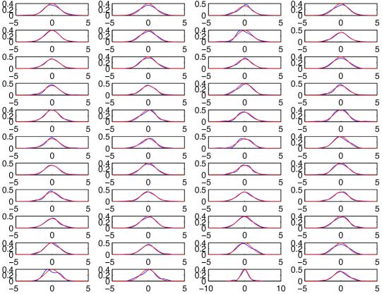
Figure 1: Graphs of the empirical density function of the transformed data versus the standard normal distribution. These graphs contain the empirical density functions of the transformed data for the first four stocks of each sector used in our study. The blue curve is the smoothed density function of the transformed data for one stock and the red curve is standard normal density function.

From these graphs, we can also see that the transformed data fit the normal density curve well. Thus from the above arguments, we can assume that the transformed data $\tilde{x}_{il}(j)$ satisfy the conditions in Theorem 1.

Now we apply $\bm{s}(\mathbf{B})$ to test the independence of every two sectors. The $p$-values are shown in Table 4. We find in the total 55 pairs of sectors, there are 23 pairs with $p$-values bigger than 0.05 and 18 pairs with $p$-values bigger than 0.1. Interestingly, according to these results, if we set the significance level as 5% we find that there are seven sectors which are independent of Sector 7, the finance and insurance sector, which seems to be most independent of other sectors. On the other hand, Sector 11 (the arts, entertainment, and recreation sector) is dependent on all other sectors except Sector 1 (the mining, quarrying, and oil and gas extraction sector). We also investigate the mutual independence of every three sectors. Applying Theorem 1, we find that there are 11 groups with $p$-values bigger than 0.05. In addtion, we find that there is only one group containing four sectors which are mutually independent. The results are shown in Table 5. Thus we have strong evidence to believe that every five sectors are dependent.

Sector	1	2	3	4	5	6	7	8	9	10
2	0.0405
3	0.0487	0.2735
4	0.0604	0	0.0002
5	0.0012	0.1041	0.0027	0.1639
6	0.0073	0.0048	0.0008	0.4285	0.0444
7	0.2299	0.4830	0.0451	0.1053	0.7080	0.6843
8	0.3558	0.0208	0.2458	0.3547	0.0013	0.0645	0.1127
9	0.1411	0.0833	0	0.0005	0.2403	0.0124	0.4521	0.0048
10	0.0418	0.3075	0.0004	0.0847	0.0746	0.0026	0.0036	0.0109	0
11	0.8689	0.0048	0	0.0470	0.0167	0.0004	0.0490	0	0.0003	0.0003

Table 4: The $p$-values obtained by the proposed test under $\mathbf{H}_{0}$ with $k=2$. Notice that the results are rounded up to the fourth decimal point.

Sectors	(1,4,8)	(1,7,8)	(1,7,9)	(2,5,7)	(2,7,9)	(4,5,7)
$p$-value	0.0804	0.1135	0.1120	0.2541	0.1413	0.1263
Sectors	(4,6,7)	(4,6,8)	(4,7,8)	(5,7,9)	(6,7,8)	(4,6,7,8)
$p$-value	0.3088	0.1277	0.0686	0.3913	0.0855	0.0650

Table 5: The $p$-values obtained by the proposed test under $\mathbf{H}_{0}$ with $k=3$ and $k=4$. Notice that the results are rounded up to the fourth decimal point.

6 Linear spectral statistics and second order freeness

In this section, we will introduce some RMT and FPT apparatus with which Theorem 1 can be proved. We will just summarize the main ideas on how these tools fit into the framework of the limiting behavior of our proposed statistic, but leave the details of the reasoning and calculation to the Appendix. We start from the following elementary fact. To wit, for two matrices $\mathbf{S}$ and $\mathbf{T}$, we know that $\mathbf{S}\mathbf{T}$ and $\mathbf{T}\mathbf{S}$ share the same non-zero eigenvalues, as long as both $\mathbf{S}\mathbf{T}$ and $\mathbf{T}\mathbf{S}$ are square. Therefore, to study the eigenvalues of $\mathbf{B}$, it is equivalent to study the eigenvalues of the $(n-1)\times(n-1)$ matrix

$$\mathbf{\underline{B}}:=\mathbf{Z}^{\prime}\text{diag}[(\mathbf{Z}_{i}\mathbf{Z}^{\prime}_{i})^{-1}]_{i=1}^{k}\mathbf{Z}=\sum_{i=1}^{k}\mathbf{Z}^{\prime}_{i}(\mathbf{Z}_{i}\mathbf{Z}^{\prime}_{i})^{-1}\mathbf{Z}_{i}.$$

Setting

$$\bm{s}(\mathbf{\underline{B}})=\frac{1}{2}\sum_{\ell=1}^{n-1}\lambda_{\ell}^{2}(\mathbf{\underline{B}})-\frac{p}{2},$$

by the above discussion we can assert

$$\bm{s}(\mathbf{\underline{B}})=\bm{s}(\mathbf{B}).$$

A main advantage of $\mathbf{\underline{B}}$ is embodied in the following proposition, which will be a starting point of the proof of Theorem 1.

Proposition 1.

Assume that $\mathbf{O}_{1},\ldots,\mathbf{O}_{k}$ are i.i.d. $(n-1)$-dimensional random orthogonal matrices possessing Haar distribution on the orthogonal group $O(n-1)$. Let $\mathbf{P}_{i}=\mathbf{I}_{p_{i}}\oplus\mathbf{0}_{n-1-p_{i}}$ be a diagonal projection matrix with rank $p_{i}$, for each $i\in\llbracket k\rrbracket$. Here we denote by $\mathbf{0}_{m}$ the $m\times m$ null matrix. Then under $\mathbf{H}_{0}$, we have

$$\underline{\mathbf{B}}\stackrel{{\scriptstyle d}}{{=}}\sum_{i=1}^{k}\mathbf{O}_{i}^{\prime}\mathbf{P}_{i}\mathbf{O}_{i}.$$

Proof.

We perform the singular value decomposition as $\mathbf{Z}_{i}:=\mathbf{U}_{i}^{\prime}\mathbf{D}_{i}\mathbf{O}_{i}$, where $\mathbf{U}_{i}$ and $\mathbf{O}_{i}$ are $p_{i}$-dimensional and $(n-1)$-dimensional orthogonal matrices respectively, and $\mathbf{D}_{i}$ is a $p_{i}\times(n-1)$ rectangular matrix whose main diagonal entries are nonzero while the others are all zero. It is well known that when $\mathbf{Z}_{i}$ has i.i.d. normal entries, both $\mathbf{U}_{i}$ and $\mathbf{O}_{i}$ are Haar distributed. Then an elementary calculation leads to Proposition 1. ∎

Note that Proposition 1 allows us to study the eigenvalues of a summation of $k$ independent random projections instead. Moreover, it is obvious that under $\mathbf{H}_{0}$, this summation of random matrices does not depend on the unknown population mean vectors and covariance matrices of $\mathbf{x}_{i}$, $i\in\llbracket k\rrbracket$.

To compress notation, we set

$$\mathbf{Q}:=\sum_{i=1}^{k}\mathbf{O}_{i}^{\prime}\mathbf{P}_{i}\mathbf{O}_{i},\quad\mathbf{Q}\stackrel{{\scriptstyle d}}{{=}}\underline{\mathbf{B}}.$$ (8)

According to the discussion in the last section, we know that our Schott type statistic can be expressed (in distribution) in terms of the eigenvalues of $\mathbf{Q}$, since

$$\text{tr}\mathbf{B}^{2}\stackrel{{\scriptstyle d}}{{=}}\text{tr}\mathbf{Q}^{2}=\sum_{\ell=1}^{n-1}\lambda_{\ell}^{2}(\mathbf{Q}).$$

In RMT, given an $N\times N$ random matrix $\mathbf{A}$ and some test function $f:\mathbb{C}\to\mathbb{C}$, one usually calls the quantity

$$\mathcal{L}_{N}[f]:=\sum_{\ell=1}^{N}f(\lambda_{\ell}(\mathbf{A}))$$

a linear spectral statistic of $\mathbf{A}$ with test function $f$. For some classical random matrix models such as Wigner matrices and sample covariance matrices, linear spectral statistics have been widely studied. Not trying to be comprehensive, one can refer to Bai and Silverstein (2004), Johansson (1998), Lytova and Pastur (2009), Sinai and Soshnikov (1998) and Shcherbina (2011) for instance. A notable feature in this type of CLTs is that usually the variance of the linear spectral statistic is of order $O(1)$ when the test function $f$ is smooth enough, mainly due to the strong correlations among eigenvalues, thus is significantly different from the case of i.i.d variables. Now, in a similar vein, with the random matrix $\mathbf{Q}$ at hand, we want to study the fluctuation of its linear spectral statistics, focusing on the test function $f(x)=x^{2}$.

In the past few decades, the main stream of RMT has focused on the spectral behavior of single random matrix models such as Wigner matrix, sample covariance matrix and non-Hermitian matrix with i.i.d. variables. However, with the rapid development in RMT and its related fields, the study of general polynomials with classical single random matrices as its variables is in increasing demand. A favorable idea is to derive the spectral properties of the matrix polynomial from the information of the spectrums of its variables (single matrices). Specifically, the question can be described as

Given the eigenvalues of $\mathbf{A}$ and $\mathbf{B}$, what can one say about the eigenvalues of $h(\mathbf{A},\mathbf{B})$?

Here $h(\cdot,\cdot)$ is a bivariate polynomial. Usually, for deterministic matrices $\mathbf{A}$ and $\mathbf{B}$, only with their eigenvalues given, it is impossible to write down the eigenvalues of $h(\mathbf{A},\mathbf{B})$. However, for some independent high-dimensional random matrices $\mathbf{A}$ and $\mathbf{B}$, deriving the limiting spectral properties of $h(\mathbf{A},\mathbf{B})$ via those of $\mathbf{A}$ and $\mathbf{B}$ is possible. To answer this kind of question, the right machinery to employ is FTP. In the breakthrough work by Voiculescu (1991), the author proved that if $(\mathbf{A}_{n})_{n\in\mathbb{N}}$ and $(\mathbf{B}_{n})_{n\in\mathbb{N}}$ are two independent sequences of random Hermitian matrices and at least one of them is orthogonally invariant (in distribution), then they satisfy the property of asymptotic freeness, which allows one to derive the limit of $\frac{1}{n}\mathbb{E}\text{tr}h(\mathbf{A}_{n},\mathbf{B}_{n})$ from the limits of $(\frac{1}{n}\mathbb{E}\text{tr}\mathbf{A}_{n}^{m})_{m\in\mathbb{N}}$ and $(\frac{1}{n}\mathbb{E}\text{tr}\mathbf{B}_{n}^{m})_{m\in\mathbb{N}}$ directly. Sometimes we also call the asymptotic freeness of two random matrix sequences as first order freeness.

Our aim in this paper, however, is not to derive the limit of the normalized trace of some polynomial in random matrices, but to take a step further to study the fluctuation of the trace. To this end, we need to adopt the concept of second order freeness, which was recently raised and developed in the series of work: Mingo and Speicher (2006); Mingo, Śniady and Speicher (2007); Collins et al. (2007); Mingo and Popa (2013), also see Redelmeier (2013). In contrast, the second order freeness aims at answering how to derive the fluctuation property of $\text{tr}h(\mathbf{A}_{n},\mathbf{B}_{n})$ from the limiting spectral properties of $\mathbf{A}_{n}$ and $\mathbf{B}_{n}$.

Especially, in Mingo and Popa (2013), the authors established the so-called real second order freeness for orthogonal matrices, which is specialized in solving the fluctuation of the linear spectral statistics of polynomials in Haar distributed orthogonal matrices and deterministic matrices. For our purpose, we need to employ Proposition 52 in Mingo and Popa (2013), an ad hoc and simplified version of which can be heuristically sketched as follows. Assume that $\{\mathbf{A}_{n}\}_{n\in\mathbb{N}}$ and $\{\mathbf{B}_{n}\}_{n\in\mathbb{N}}$ are two independent sequences of random matrices (may be deterministic), where $\mathbf{A}_{n}$ and $\mathbf{B}_{n}$ are $n$ by $n$, and the limits of $n^{-1}\mathbb{E}\text{tr}h_{1}(\mathbf{A}_{n})$ and $n^{-1}\mathbb{E}\text{tr}h_{2}(\mathbf{B}_{n})$ exist for any given polynomials $h_{1}$ and $h_{2}$, as $n\to\infty$. Moreover, $\text{tr}h_{1}(\mathbf{A}_{n})$ and $\text{tr}h_{2}(\mathbf{B}_{n})$ possess Gaussian fluctuations (may be degenerate) asymptotically for any given polynomials $h_{1}$ and $h_{2}$. Then $\text{tr}q(\mathbf{O}^{\prime}\mathbf{A}_{n}\mathbf{O},\mathbf{B}_{n})$ also possesses Gaussian fluctuation asymptotically for any given bivariate polynomial $q(\cdot,\cdot)$, where $\mathbf{O}$ is supposed to be an $n\times n$ Haar orthogonal matrix independent of $\mathbf{A}_{n}$ and $\mathbf{B}_{n}$.

Now as for $\mathbf{Q}$, we can start from the case of $k=2$, which fits the above framework quite well. To wit, we can regard $\mathbf{O}_{1}^{\prime}\mathbf{P}_{1}\mathbf{O}_{1}$ as $\mathbf{B}_{n-1}$ and $\mathbf{P}_{2}$ as $\mathbf{A}_{n-1}$, using Proposition 52 of Mingo and Popa (2013) leads to the fact that $\text{tr}h(\mathbf{O}_{1}^{\prime}\mathbf{P}_{1}\mathbf{O}_{1}+\mathbf{O}_{2}^{\prime}\mathbf{P}_{2}\mathbf{O}_{2})$ is asymptotically Gaussian after an appropriate normalization, for any given polynomial $h$. Then we take $\mathbf{O}_{1}^{\prime}\mathbf{P}_{1}\mathbf{O}_{1}+\mathbf{O}_{2}^{\prime}\mathbf{P}_{2}\mathbf{O}_{2}$ as $\mathbf{B}_{n-1}$ and regard $\mathbf{P}_{3}$ as $\mathbf{A}_{n-1}$ and repeat the above discussion. By using Proposition 52 in Mingo and Popa (2013) recursively, we can get our CLT for $\mathbf{Q}$ finally. A formal result which can be derived from Proposition 52 in Mingo and Popa (2013) is as follows, whose proof will be presented in the Appendix.

Theorem 2.

For our matrix $\mathbf{Q}$ defined in (8), and any deterministic polynomial sequence $h_{1},h_{2},$ $h_{3},\cdots$, we have

$$\text{Cov}(\text{tr }h_{1}(\mathbf{Q}),\text{tr }h_{2}(\mathbf{Q}))=O(1)$$

and

$$\lim_{n\to\infty}\kappa_{r}(\text{tr }h_{1}(\mathbf{Q}),\ldots,\text{tr }h_{r}(\mathbf{Q}))=0,\quad\text{if }r\geq 3$$

where $\kappa_{r}(\xi_{1},\ldots,\xi_{r})$ represents the joint cumulant of the random variables $\xi_{1},\ldots,\xi_{r}$.

Now if we set $h_{i}(x)=x^{2}$ for all $i\in\mathbb{N}$, we can obtain Theorem 1 by proving the following lemma.

Lemma 1.

Under the above notation, we have

$$\mathbb{E}\text{tr}\mathbf{Q}^{2}=p+\sum_{\begin{subarray}{c}i,j,i\neq j\end{subarray}}\frac{p_{i}p_{j}}{n-1},$$ (9)

and

$$\text{Var}(\text{tr}\mathbf{Q}^{2})=4\sum_{\begin{subarray}{c}i,j,i\neq j\end{subarray}}\frac{p_{i}p_{j}(n-1-p_{i})(n-1-p_{j})}{(n-1)^{4}}+O(\frac{1}{n}).$$ (10)

The proof of Lemma 1 will also be stated in the Appendix. In the sequel, we prove Theorem 1 with Lemma 1 granted.

Proof of Theorem 1. Setting $h_{i}(x)=x^{2}$ for all $i\in\mathbb{N}$ in Theorem 2, we see that all $r$th cumulants of $\text{tr}\mathbf{Q}^{2}$ tend to $0$ if $r\geq 3$ when $n\to\infty$, which together with Lemma 1 implies that

$$\frac{\text{tr}\mathbf{Q}^{2}-\mathbb{E}\text{tr}\mathbf{Q}^{2}}{\sqrt{\text{Var}(\text{tr}\mathbf{Q}^{2})}}\Longrightarrow N(0,1).$$

Then Theorem 1 follows from the definition of $\mathbf{s}(\mathbf{B})$ directly. ∎

Appendix

In this Appendix, we provide the proofs of Theorem 2 and Lemma 1.

Proof of Theorem 2. In Proposition 52 of Mingo and Popa (2013), the authors state that if $\{\mathbf{A}_{n}\}_{n\in\mathbb{N}}$ and $\{\mathbf{B}_{n}\}_{n\in\mathbb{N}}$ are two independent sequences of random matrices (may be deterministic), where $\mathbf{A}_{n}$ and $\mathbf{B}_{n}$ are $n\times n$, each having a real second order limit distribution, and $\mathbf{O}$ is supposed to be an $n\times n$ Haar orthogonal matrix independent of $\mathbf{A}_{n}$ and $\mathbf{B}_{n}$, then $\mathbf{B}_{n}$ and $\mathbf{O}^{\prime}\mathbf{A}_{n}\mathbf{O}$ are asymptotically real second order free. By Definition 30 of Mingo and Popa (2013), we see that for a single random matrix sequence $\{\mathbf{A}_{n}\}_{n\in\mathbb{N}}$, the existence of the so-called real second order limit distribution means that the following three statements hold simultaneously for any given sequence of polynomials $h_{1},h_{2},h_{3},\ldots$ when $n\to\infty$:

1. $n^{-1}\mathbb{E}\text{tr}h_{1}(\mathbf{A}_{n})$ converges;

2. $\text{Cov}(\text{tr}h_{1}(\mathbf{A}_{n}),\text{tr}h_{2}(\mathbf{A}_{n}))$ converges (the limit can be $0$);

3. $\kappa_{r}(\text{tr}h_{1}(\mathbf{A}_{n}),\ldots,\text{tr}h_{r}(\mathbf{A}_{n}))=o(1)$ for all $r\geq 3$.

We stress here, the original definition in Mingo and Popa (2013) is given with a language of non-commutative probability theory. To avoid introducing too many additional notions, we just modify it to be the above 1)-3). Then by the Definition 33 and Proposition 52 of Mingo and Popa (2013)), one see that if both $\{\mathbf{A}_{n}\}_{n\in\mathbb{N}}$ and $\{\mathbf{B}_{n}\}_{n\in\mathbb{N}}$ have real second order limit distributions, we have the following three facts for any given sequences of bivariate polynomials $q_{1},q_{2},q_{3},\ldots$ when $n\to\infty$:

1. $n^{-1}\mathbb{E}\text{tr}q_{1}(\mathbf{B}_{n},\mathbf{O}^{\prime}\mathbf{A}_{n}\mathbf{O})$ converges;

2. $\text{Cov}(\text{tr}q_{1}(\mathbf{B}_{n},\mathbf{O}^{\prime}\mathbf{A}_{n}\mathbf{O}),\text{tr}q_{2}(\mathbf{B}_{n},\mathbf{O}^{\prime}\mathbf{A}_{n}\mathbf{O}))$ converges;

3. $\kappa_{r}(\text{tr}q_{1}(\mathbf{B}_{n},\mathbf{O}^{\prime}\mathbf{A}_{n}\mathbf{O}),\ldots,\text{tr}q_{r}(\mathbf{B}_{n},\mathbf{O}^{\prime}\mathbf{A}_{n}\mathbf{O}))=o(1)$ for all $r\geq 3$.

Here 1’) and 2’) can be implied by the definitions of the first and second order freeness in Mingo and Popa (2013) respectively, and 3’) can be found in the proof of Proposition 52 of Mingo and Popa (2013), where the authors claim that the proof of Theorem 41 therein is also applicable under the setting of Proposition 52. Note that in Mingo and Popa (2013), a more concrete rule to determine the limit of $\text{Cov}(\text{tr}q_{1}(\mathbf{B}_{n},\mathbf{O}^{\prime}\mathbf{A}_{n}\mathbf{O}),\text{tr}q_{2}(\mathbf{B}_{n},\mathbf{O}^{\prime}\mathbf{A}_{n}\mathbf{O}))$ is given, which can be viewed as the core of the concept of real second order freeness. However, here we do not need such a concrete rule, thus do not introduce it.

Now we are at the stage of employing Proposition 52 of Mingo and Popa (2013) to prove Theorem 2. Recall our objective $\mathbf{Q}$ defined in (8). We start from the case of $k=2$, to wit, we are considering the linear spectral statistics of the random matrix $\mathbf{O}_{1}^{\prime}\mathbf{P}_{1}\mathbf{O}_{1}+\mathbf{O}_{2}^{\prime}\mathbf{P}_{2}\mathbf{O}_{2}$. Now, we regard $\mathbf{O}_{1}^{\prime}\mathbf{P}_{1}\mathbf{O}_{1}$ as $\mathbf{B}_{n-1}$ and $\mathbf{P}_{2}$ as $\mathbf{A}_{n-1}$, then obviously they both satisfy 1)-3) in the definition of the existence of the real second order limit distribution, since the spectrums of $\mathbf{A}_{n-1}$ and $\mathbf{B}_{n-1}$ are both deterministic, noticing they are projection matrices with known ranks. Then 1’)-3’) immediately imply that $\mathbf{O}_{1}^{\prime}\mathbf{P}_{1}\mathbf{O}_{1}+\mathbf{O}_{2}^{\prime}\mathbf{P}_{2}\mathbf{O}_{2}$ also has a real second order limit distribution. Next, adding $\mathbf{O}_{3}^{\prime}\mathbf{P}_{3}\mathbf{O}_{3}$ to $\mathbf{O}_{1}^{\prime}\mathbf{P}_{1}\mathbf{O}_{1}+\mathbf{O}_{2}^{\prime}\mathbf{P}_{2}\mathbf{O}_{2}$, and regarding the latter as $\mathbf{B}_{n-1}$ and $\mathbf{P}_{3}$ as $\mathbf{A}_{n-1}$, we can use the above discussion again to conclude that $\mathbf{O}_{1}^{\prime}\mathbf{P}_{1}\mathbf{O}_{1}+\mathbf{O}_{2}^{\prime}\mathbf{P}_{2}\mathbf{O}_{2}+\mathbf{O}_{3}^{\prime}\mathbf{P}_{3}\mathbf{O}_{3}$ also possesses a real second order limit distribution. Recursively, we can finally get that $\mathbf{Q}$ has a real second order limit distribution, which implies Theorem 2. So we conclude the proof. ∎

It remains to prove Lemma 1. Before commencing the proof, we briefly introduce some technical inputs. Since the trace of a product of matrices can always be expressed in terms of some products of their entries, it is expected that we will need to calculate the quantities of the form

$$\mathbb{E}\mathbf{O}_{i_{1}j_{1}}\cdots\mathbf{O}_{i_{m}j_{m}},$$ (11)

where $\mathbf{O}$ is assumed to be an $N$-dimensional Haar distributed orthogonal matrix, and $\mathbf{O}_{ij}$ is its $(i,j)$th entry. A powerful tool handling this kind of expectation is the so-called Weingarten calculus on orthogonal group, we refer to the seminal paper of Collins and Śniady (2006), formula (21) therein. To avoid introducing too many combinatorics notions for Weingarten calculus, we just list some consequence of it for our purpose, taking into account the fact that we will only need to handle the case of $m\leq 4$ in (11) in the sequel. Specifically, we have the following lemma.

Lemma 2.

Under the above notation, we have the following facts for (11), assuming $m\leq 4$ and $\mathbf{i}=(i_{1},\ldots,i_{m})$ and $\mathbf{j}=(j_{1},\ldots,j_{m})$.

1): When $m=2$, $i_{1}=i_{2}$, and $j_{1}=j_{2}$, we have $(\ref{052701})=N^{-1}$,

2): When $m=4$, we have the following results for four sub-cases.

1. If $i_{1}=i_{2}=i_{3}=i_{4}$, $j_{1}=j_{2}=j_{3}=j_{4}$, we have $(\ref{052701})=3/(N(N+2))$;
   

2. If $i_{1}=i_{2}=i_{3}=i_{4}$, $j_{1}=j_{2}\neq j_{3}=j_{4}$, we have $(\ref{052701})=1/(N(N+2))$;
   

3. If $i_{1}=i_{2}\neq i_{3}=i_{4}$, $j_{1}=j_{2}\neq j_{3}=j_{4}$, we have $(\ref{052701})=(N+1)/(N(N-1)(N+2))$;
   

4. If $i_{1}=i_{3}\neq i_{2}=i_{4}$, $j_{1}=j_{2}\neq j_{3}=j_{4}$, we have $(\ref{052701})=-1/(N(N-1)(N+2))$.

3): Replacing $\mathbf{O}$ by $\mathbf{O}^{\prime}$, we can obviously switch the roles of $\mathbf{i}$ and $\mathbf{j}$ in 1) and 2). Moreover, any permutation on the indices $\{1,\ldots,m\}$ will not change (11). Any other triple $(m,\mathbf{i},\mathbf{j})$, which can not be transformed into any case in 1) or 2) via switching the roles of $\mathbf{i}$ and $\mathbf{j}$ or performing permutations on the indices $\{1,\ldots,m\}$, will drives (11) to be $0$.

With Lemma 2 at hand, we can prove Lemma 1 in the sequel.

Proof of Lemma 1. At first, we verify (9). Note that by definition,

$$\mathbb{E}\text{tr}\mathbf{Q}^{2} = \sum_{i=1}^{k}\mathbb{E}\text{tr}(\mathbf{O}_{i}^{\prime}\mathbf{P}_{i}\mathbf{O}_{i})^{2}+\sum_{\begin{subarray}{c}i,j,i\neq j\end{subarray}}\mathbb{E}\text{tr}(\mathbf{O}_{i}^{\prime}\mathbf{P}_{i}\mathbf{O}_{i}\cdot\mathbf{O}_{j}^{\prime}\mathbf{P}_{j}\mathbf{O}_{j})$$

$$= p+\sum_{\begin{subarray}{c}i,j,i\neq j\end{subarray}}\mathbb{E}\text{tr}(\mathbf{O}_{i}^{\prime}\mathbf{P}_{i}\mathbf{O}_{i}\cdot\mathbf{O}_{j}^{\prime}\mathbf{P}_{j}\mathbf{O}_{j}).$$

Let $\mathbf{u}_{i}(\ell)$ be the $\ell$th column of $\mathbf{O}_{i}^{\prime}$ and $\mathbf{u}_{i}(\ell,s)$ be the $s$th coefficient of $\mathbf{u}_{i}(\ell)$, i.e. the $(\ell,s)$th entry of $\mathbf{O}_{i}$, for all $i\in\llbracket k\rrbracket$. Then for $i\neq j$ we have

$$\mathbb{E}\text{tr}(\mathbf{O}_{i}^{\prime}\mathbf{P}_{i}\mathbf{O}_{i}\cdot\mathbf{O}_{j}^{\prime}\mathbf{P}_{j}\mathbf{O}_{j}) = \mathbb{E}\sum_{m=1}^{p_{i}}\sum_{\ell=1}^{p_{j}}\text{tr}\mathbf{u}_{i}(m)\mathbf{u}_{i}^{\prime}(m)\mathbf{u}_{j}(\ell)\mathbf{u}_{j}^{\prime}(\ell)$$ (12)

$$= \sum_{m=1}^{p_{i}}\sum_{\ell=1}^{p_{j}}\sum_{s}\sum_{t}\mathbb{E}\mathbf{u}_{i}(m,s)\mathbf{u}_{i}(m,t)\cdot\mathbb{E}\mathbf{u}_{j}(\ell,s)\mathbf{u}_{j}(\ell,t)$$

$$= \sum_{m=1}^{p_{i}}\sum_{\ell=1}^{p_{j}}\sum_{s}\mathbb{E}(\mathbf{u}_{i}(m,s))^{2}\mathbb{E}(\mathbf{u}_{j}(\ell,s))^{2}=\frac{p_{i}p_{j}}{n-1}.$$

Here, in the third step above we used 3) of Lemma 2 to discard the terms with $s\neq t$, while in the last step we used 1) of Lemma 2. Therefore, we have

$$\mathbb{E}\text{tr}(\sum_{i=1}^{k}\mathbf{O}_{i}^{\prime}\mathbf{P}_{i}\mathbf{O}_{i})^{2}=p+\sum_{\begin{subarray}{c}i,j,i\neq j\end{subarray}}\frac{p_{i}p_{j}}{n-1},$$ (13)

Now we calculate $\text{Var}(\text{tr}\mathbf{Q}^{2})$ as follows. Note that we have

$$\text{Var}(\text{tr}\mathbf{Q}^{2}) = \mathbb{E}(\text{tr}(\sum_{i=1}^{k}\mathbf{O}_{i}^{\prime}\mathbf{P}_{i}\mathbf{O}_{i})^{2})^{2}-(\mathbb{E}\text{tr}(\sum_{i=1}^{k}\mathbf{O}_{i}^{\prime}\mathbf{P}_{i}\mathbf{O}_{i})^{2})^{2}$$

$$= \mathbb{E}\bigg{(}\sum_{\begin{subarray}{c}i,j,i\neq j\end{subarray}}\text{tr}(\mathbf{O}_{i}^{\prime}\mathbf{P}_{i}\mathbf{O}_{i}\cdot\mathbf{O}_{j}^{\prime}\mathbf{P}_{j}\mathbf{O}_{j})\bigg{)}^{2}-\bigg{(}\mathbb{E}\sum_{\begin{subarray}{c}i,j,i\neq j\end{subarray}}\text{tr}(\mathbf{O}_{i}^{\prime}\mathbf{P}_{i}\mathbf{O}_{i}\cdot\mathbf{O}_{j}^{\prime}\mathbf{P}_{j}\mathbf{O}_{j})\bigg{)}^{2}$$

$$= \sum_{\begin{subarray}{c}i,j,i\neq j\end{subarray}}\sum_{\begin{subarray}{c}m,\ell,m\neq\ell\end{subarray}}\text{Cov}(\text{tr}(\mathbf{O}_{i}^{\prime}\mathbf{P}_{i}\mathbf{O}_{i}\cdot\mathbf{O}_{j}^{\prime}\mathbf{P}_{j}\mathbf{O}_{j}),\text{tr}(\mathbf{O}_{m}^{\prime}\mathbf{P}_{m}\mathbf{O}_{m}\cdot\mathbf{O}_{\ell}^{\prime}\mathbf{P}_{\ell}\mathbf{O}_{\ell}))$$

$$= \sum_{\begin{subarray}{c}i,j,m,\ell\\ i\neq j,m\neq\ell\\ \{i,j\}\cap\{m,\ell\}\neq\emptyset\end{subarray}}\text{Cov}(\text{tr}(\mathbf{O}_{i}^{\prime}\mathbf{P}_{i}\mathbf{O}_{i}\cdot\mathbf{O}_{j}^{\prime}\mathbf{P}_{j}\mathbf{O}_{j}),\text{tr}(\mathbf{O}_{m}^{\prime}\mathbf{P}_{m}\mathbf{O}_{m}\cdot\mathbf{O}_{\ell}^{\prime}\mathbf{P}_{\ell}\mathbf{O}_{\ell})).$$

In the sequel, we briefly write

$$\text{Cov}((i,j),(m,\ell)):=\text{Cov}(\text{tr}(\mathbf{O}_{i}^{\prime}\mathbf{P}_{i}\mathbf{O}_{i}\cdot\mathbf{O}_{j}^{\prime}\mathbf{P}_{j}\mathbf{O}_{j}),\text{tr}(\mathbf{O}_{m}^{\prime}\mathbf{P}_{m}\mathbf{O}_{m}\cdot\mathbf{O}_{\ell}^{\prime}\mathbf{P}_{\ell}\mathbf{O}_{\ell}))$$

Note that the summation in the last step above can be decomposed into the following six cases.

$$1:m=i,\quad\ell=j;\qquad\hskip 8.61108pt2:m=j,\quad\ell=i;$$

$$3:m=i,\quad\ell\neq i,j;\qquad 4:\ell=i,\quad m\neq i,j;$$

$$5:m=j,\quad\ell\neq i,j;\qquad 6:\ell=j,\quad m\neq i,j.$$

Now given $i,j$, we decompose the summation over $m,\ell$ according to the above $6$ cases and denote the sum restricted on these cases by $\sum_{\alpha(i,j)},\alpha(i,j)=1,\ldots,6$ respectively. Therefore,

$$\text{Var}(\text{tr}\mathbf{Q}^{2})=\sum_{\begin{subarray}{c}i,j,i\neq j\end{subarray}}\sum_{\alpha(i,j)=1}^{6}\sum\nolimits_{\alpha(i,j)}\text{Cov}((i,j),(m,\ell))$$ (14)

Now by definition we have

$$\sum_{\begin{subarray}{c}i,j,i\neq j\end{subarray}}\sum\nolimits_{\alpha(i,j)}\text{Cov}((i,j),(m,\ell))=\sum_{i}\sum_{j\neq i}\text{Cov}((i,j),(i,j)),\qquad\hskip 4.30554pt\alpha=1,2,$$

$$\sum_{\begin{subarray}{c}i,j,i\neq j\end{subarray}}\sum\nolimits_{\alpha(i,j)}\text{Cov}((i,j),(m,\ell))=\sum_{i}\sum_{j\neq i}\sum_{\ell\neq i,j}\text{Cov}((i,j),(i,\ell)),\quad\alpha=3,4,$$

$$\sum_{\begin{subarray}{c}i,j,i\neq j\end{subarray}}\sum\nolimits_{\alpha(i,j)}\text{Cov}((i,j),(m,\ell))=\sum_{i}\sum_{j\neq i}\sum_{\ell\neq i,j}\text{Cov}((i,j),(j,\ell)),\quad\alpha=5,6.$$

Now note that for $i\neq j$

$$\text{Cov}((i,j),(i,j)) = \mathbb{E}(\text{tr}(\mathbf{O}_{i}^{\prime}\mathbf{P}_{i}\mathbf{O}_{i}\cdot\mathbf{O}_{j}^{\prime}\mathbf{P}_{j}\mathbf{O}_{j}))^{2}-(\mathbb{E}\text{tr}(\mathbf{O}_{i}^{\prime}\mathbf{P}_{i}\mathbf{O}_{i}\cdot\mathbf{O}_{j}^{\prime}\mathbf{P}_{j}\mathbf{O}_{j}))^{2}$$

$$= \mathbb{E}(\text{tr}(\mathbf{O}_{i}^{\prime}\mathbf{P}_{i}\mathbf{O}_{i}\cdot\mathbf{O}_{j}^{\prime}\mathbf{P}_{j}\mathbf{O}_{j}))^{2}-(\frac{p_{i}p_{j}}{n-1})^{2},$$

where the last step follows from (12). Moreover, we have

$$\mathbb{E}(\text{tr}(\mathbf{O}_{i}^{\prime}\mathbf{P}_{i}\mathbf{O}_{i}\cdot\mathbf{O}_{j}^{\prime}\mathbf{P}_{j}\mathbf{O}_{j}))^{2}$$

$$=\sum_{m_{1},m_{2}=1}^{p_{i}}\sum_{\ell_{1},l_{2}=1}^{p_{j}}\mathbb{E}\mathbf{u}_{i}^{\prime}(m_{1})\mathbf{u}_{j}(\ell_{1})\mathbf{u}_{j}^{\prime}(\ell_{1})\mathbf{u}_{i}(m_{1})\mathbf{u}_{i}^{\prime}(m_{2})\mathbf{u}_{j}(\ell_{2})\mathbf{u}_{j}^{\prime}(\ell_{2})\mathbf{u}_{i}(m_{2})$$

$$=\sum_{s_{1},s_{2},t_{1},t_{2}}\bigg{[}\sum_{m_{1},m_{2}=1}^{p_{i}}\mathbb{E}\mathbf{u}_{i}(m_{1},s_{1})\mathbf{u}_{i}(m_{1},t_{1})\mathbf{u}_{i}(m_{2},s_{2})\mathbf{u}_{i}(m_{2},t_{2})\bigg{]}$$

$$\hskip 64.58313pt\times\bigg{[}\sum_{\ell_{1},\ell_{2}=1}^{p_{j}}\mathbb{E}\mathbf{u}_{j}(\ell_{1},s_{1})\mathbf{u}_{j}(\ell_{1},t_{1})\mathbf{u}_{j}(\ell_{2},s_{2})\mathbf{u}_{j}(\ell_{2},t_{2})\bigg{]}.$$

To calculate the above expectation, we need to use Lemma 2 again. In light of 3) of Lemma 2, it suffices to consider the following four cases

$$1:s_{1}=s_{2}=t_{1}=t_{2},\quad 2:s_{1}=s_{2}\neq t_{1}=t_{2}$$

$$3:s_{1}=t_{1}\neq s_{2}=t_{2},\quad 4:s_{1}=t_{2}\neq s_{2}=t_{1}.$$

Through detailed but elementary calculation, with the aid of Lemma 2, we can finally obtain that for $i\neq j$,

$$\text{Cov}((i,j),(i,j))=\frac{2p_{i}p_{j}(n-1-p_{i})(n-1-p_{j})}{(n-1)^{4}}+O(\frac{1}{n}).$$

Moreover, analogously, when $i,j,\ell$ are mutually distinct, we can get

$$\text{Cov}((i,j),(i,\ell))=\text{Cov}((i,j),(j,\ell))=O(\frac{1}{n})$$

by using Lemma 2. Here we just omit the details of the calculation. Consequently, by (14) one has

$$\text{Var}(\text{tr}\mathbf{Q}^{2})=\sum_{\begin{subarray}{c}i,j,i\neq j\end{subarray}}\frac{4p_{i}p_{j}(n-1-p_{i})(n-1-p_{j})}{(n-1)^{4}}+O(\frac{1}{n}).$$ (15)

Thus we conclude the proof. ∎

References

• Anderson (2003) Anderson, T. (2003). An introduction to multivariate statistical analysis. Third Edition. Wiley New York.
• Bai et al. (2009) Bai, Z. D., Jiang, D. D., Yao, J. F. and Zheng, S. R. (2009). Corrections to LRT on large-dimensional covariance matrix by RMT. Ann. Statist.37(6B), 3822-3840.
• Bai and Silverstein (2004) Bai, Z. D., Silverstein, J. W. (2004). CLT for linear spectral statistics of large-dimensional sample covariance matrices. Ann. Probab., 32(1A), 553-605.
• Cai and Jiang (2011) Cai, T. T. and Jiang, T. F.(2011). Limiting laws of coherence of random matrices with applications to testing covariance structure and construction of compressed sensing matrices. Ann. Statist. 39(3), 1496-1525.
• Collins et al. (2007) Collins, B., Mingo, J. A., ลšniady, P. and Speicher, R.(2007). Second order freeness and fluctuations of Random Matrices: III. Higher order freeness and free cumulants, Doc. Math., 12, 1-70.
• Collins and ลšniady (2006) Collins, B. and ลšniady, P. (2006). Integration with respect to the Haar measure on unitary, orthogonal and symplectic group. Commun. Math. Phys. 264, 773-795.
• Jiang, Bai and Zheng (2013) Jiang D. D., Bai Z. D., Zheng S. R. (2013). Testing the independence of sets of large-dimensional variables. Science China Mathematics, 56(1), 135-147.
• Jiang and Yang (2013) Jiang T. F. and Yang F. (2013). Central limit theorems for classical likelihood ratio tests for high-dimensional normal distributions. Ann. Statist., 41(4),2029-2074.
• Johansson (1998) Johansson, K. (1998). On fluctuations of eigenvalues of random Hermitian matrices. Duke Math. J., 91, 151-204.
• Mingo and Popa (2013) Mingo J. A., Popa M. (2013). Real second order freeness and Haar orthogonal matrices. J. Math. Phys., 54(5), 051701.
• Mingo and Speicher (2006) Mingo, J. A., Speicher, R. (2006). Second order freeness and fluctuations of random matrices: I. Gaussian and Wishart matrices and cyclic Fock spaces. Journal of Functional Analysis, 235(1), 226-270.
• Mingo, ลšniady and Speicher (2007) Mingo, J. A., ลšniady, P. and Speicher. R. (2007). Second order freeness and fluctuations of random matrices: II. Unitary random matrices. Advances in Mathematics, 209(1), 212-240.
• Muirhead (1982) Muirhead, R. J. (1982). Aspects of Multivariate Statistical Theory. Wiley, New York.
• Johnstone (2001) Johnstone, I. M.(2001). On the distribution of the largest eigenvalue in principal components analysis. Ann. Statist. 29, 295-327.
• Ledoit and Wolf (2002) Ledoit, O. and Wolf, M.(2002). Some hypothesis tests for the covariance matrix when the dimension is large compared to the sample size. Ann. Statist. 30, 1081-1102.
• Lytova and Pastur (2009) Lytova, A., Pastur, L.. Central limit theorem for linear eigenvalue statistics of random matrices with independent entries. Ann. Probab., 37(5), 1778-1840.
• Pearson (1900) Pearson, Karl (1900). On the criterion that a given system of deviations from the probable in the case of a correlated system of variables is such that it can be reasonably supposed to have arisen from random sampling. Philosophical Magazine Series 5 50(302), 157-175.
• Rama (2001) Rama, C. (2001). Empirical properties of asset returns: stylized facts and statistical issues. Quant. Finance 1, 223-236.
• Rao et al. (2008) Rao, N. R., Mingo, J. A., Speicher, R. and Edelman, A. (2008). Statistical eigen-inference from large Wishart matrices. Ann. Statist., 2850-2885.
• Redelmeier (2013) Redelmeier, E. (2013). Real Second-Order Freeness and the Asymptotic Real Second-Order Freeness of Several Real Matrix Models. Int. Math. Res. Notices, doi: 10.1093/imrn/rnt043
• Schott (2005) Schott, J. R.(2005). Testing for complete independence in high dimensions. Biometrika 92, 951-956.
• Shcherbina (2011) Shcherbina, M.(2011). Central limit theorem for linear eigenvalue statistics of the Wigner and sample covariance random matrices. Math. Phys. Anal. Geom., 7(2), 176-192.
• Srivastava (2005) Srivastava, M. S. (2005) Some Tests Concerning the Covariance Matrix in High Dimensional Data. Journal of the Japan Statistical Society, 35(2):251โ€“272.
• Sinai and Soshnikov (1998) Sinai, Y., Soshnikov, A. (1998). Central limit theorem for traces of large random symmetric matrices with independent matrix elements. Bol. Soc. Brasil. Mat.29(1), 1-24.
• Voiculescu (1991) Voiculescu, D. (1991). Limit laws for random matrices and free products. Invent. Math., 104(1), 201-220.
• Wilks (1935) Wilks, S. S. (1935). On the independence of k sets of normally distributed statistical variables. Econometrica 3, 309-326.