Diffraction Patterns of Layered Close-packed Structures
from Hidden Markov Models

Abstract

We recently derived analytical expressions for the pairwise (auto)correlation functions (CFs) between modular layers (MLs) in close-packed structures (CPSs) for the wide class of stacking processes describable as hidden Markov models (HMMs) [Riechers et al., (2014), Acta Crystallogr. A, XX 000-000]. We now use these results to calculate diffraction patterns (DPs) directly from HMMs, discovering that the relationship between the HMMs and DPs is both simple and fundamental in nature. We show that in the limit of large crystals, the DP is a function of parameters that specify the HMM. We give three elementary but important examples that demonstrate this result, deriving expressions for the DP of CPSs stacked (i) independently, (ii) as infinite-Markov-order randomly faulted 2H and 3C stacking structures over the entire range of growth and deformation faulting probabilities, and (iii) as a HMM that models Shockley-Frank stacking faults in 6H-SiC. While applied here to planar faulting in CPSs, extending the methods and results to planar disorder in other layered materials is straightforward. In this way, we effectively solve the broad problem of calculating a DP—either analytically or numerically—for any stacking structure—ordered or disordered—where the stacking process can be expressed as a HMM.

I Introduction

Increasingly, materials scientists appreciate the sometimes unexpected role that disorder and crystal defects play in material properties. Crystal defects have, of course, been known and studied for some time, Hirth and Lothe (1968) but in the past they have often been viewed as a nuisance or feature to be minimized or eliminated. Caroff et al. (2011) However, as material scientists acquired the ability to engineer the composition and structure of materials at the nanoscale level, Geim and Grigorieva (2013) they have concomitantly discovered that disorder, far from being unwelcome, can result in specimens with desirable material properties. For example, the introduction of defects into graphene nanosheets improves their performance in batteries, Pan et al. (2009) and so-called ‘defect engineering’ in semiconductors is attracting wide attention. Seebauer and Noh (2010)

The growing technological import of disordered materials then challenges the crystallographic community to develop a theoretical framework capable of discovering, describing, and quantifying the noncrystallinity so often present in condensed matter systems. While concepts such as the Bravais lattice and point and space groups have allowed for the classification and codification of perfectly ordered materials, a new formalism—founded on concepts and mathematical constructs that intrinsically treat nonzero entropy systems—is needed. A. L. Mackay (1986); Cartwright and Mackay (2012) For quasi-one-dimensional materials, this formalism has been identified: chaotic crystallography (ChC). Varn and Crutchfield (2014)

ChC is the use of information- and computation-theoretic methods to discover, describe, and categorize material structure. Specifically, it adapts and applies computational mechanics Crutchfield (2012); Shalizi and Crutchfield (2001) to the problem of disorder in materials. Drawing from concepts developed in information theory, Cover and Thomas (2006) theoretical computer science Paz (1971); Hopcroft and Ullman (1979) and nonlinear dynamics, Strogatz (2001); Feldman (2012) computational mechanics has been successfully applied to a number of physical systems. Palmer et al. (2000); Clarke et al. (2003); Kelly et al. (2012)

While many kinds of disorder may be present in materials, here we restrict our attention to the disorder that results from shifting or displacing an entire plane of atoms. We assume that the three-dimensional material is built up from the stacking of identical, crystalline, two-dimensional layers, which here we refer to as modular layers (MLs). Price (1983); Ferraris et al. (2008) There are usually constraints on the allowed alignment between adjacent MLs, effectively restricting to a small set the number of possible ML orientations. Thus, a complete description of a quasi-one-dimensional disordered specimen reduces to a one-dimensional list of the successive orientations of the MLs encountered as one moves along the stacking direction, called the stacking sequence. Varn et al. (2002) The effective stochastic process induced by scanning the stacking sequence is referred to as the stacking process. Varn et al. (2002)

For specimens containing many MLs, listing the entire stacking sequence can be cumbersome, as well as unnecessary. Since many properties of disordered materials depend not on the specific stacking sequence, but rather on the statistics of the stacking sequence—i.e., the stacking process—ChC conveniently specifies material structure in terms the hidden Markov model (HMM) that describes the stacking process. We contend that any quantity depending on the statistics of the stacking process should be amenable to direct calculation from the process’s HMM. Indeed, it has recently been shown Riechers et al. (2014) that the pairwise (auto)correlation functions between MLs are directly calculable from the HMM. However, until now, several quantities, such as the diffraction pattern (DP), have defied exact calculation from a general HMM. Of course, the difficulty of estimating DPs from models of disordered stackings predates the use of HMMs. In fact, there is a considerable literature devoted to deriving expressions for the DP for faulted specimens or special cases of disorder. Hendricks and Teller (1942); Wilson (1942); Kakinoki and Komura (1965); Holloway and Klamkin (1969); Holloway (1969); Pandey et al. (1980a, b, c); Sebastian and Krishna (1994); Gosk (2001); Kopp et al. (2012) Finite-order Markov processes have a formal solution in the work following Hendricks and Teller Hendricks and Teller (1942) and Kakinoki and Komura Kakinoki and Komura (1965), but even simple examples with two coexisting faulting mechanisms transcend the limitations of these methods. Researchers typically work out the consequences for particular models, but a general theory has been elusive.

To circumvent the often tedious algebra innate to these analytical techniques, Berliner and Werner Berliner and Werner (1986) demonstrated that CFs and thereby the DP could be explicitly calculated by taking a sample stacking sequence derived from a particular model of disorder. Though now in common usage, this approach is not altogether satisfactory. The first difficulty lies in the statistical fluctuations inherent from considering any finite-size sample. It is known that these statistical fluctuations lead to fluctuations in the power spectrum that are on the order of the magnitude of the power spectrum itself. Kantz and Schreiber (2004) This difficulty can be ameliorated by taking many samples and averaging Nikolin and Babkevich (1989) or by using a smoothing procedure. Varn (2001); Varn et al. (2013a) The second challenge may seem perhaps more ascetic, but the objection is firmly grounded in the difficulty that arises when using the approach to compare experimentally obtained DPs with calculated ones; as is necessary in many estimation algorithms, such as reverse Monte Carlo modeling, Keen and McGreevy (1990) and differential evolution and genetic algorithms. Michels-Clark et al. (2013)

There are additional advantages to expressing the DP as an analytical function of the HMM. For example, if analytical expressions for the DP of an arbitrary HMM become available, then a systematic search of all HMM architectures up to a given number of states becomes feasible. Johnson et al. (2010); Strelioff and Crutchfield (2014) This makes it possible to infer long-range structures in the so-called strictly sofic processes Paz (1971); Badii and Politi (1997) directly from X-ray diffraction studies. Simulation studies suggest that the sofic stacking processes, which possess a kind of infinite memory and hence cannot be represented by any finite-order Markov model, may be important in solid-state transformations. Varn and Crutchfield (2004) More broadly, we expect that exploring analytical methods will lead to expressions for material properties, such as electrical conductivities and band structures, in terms of HMM parameters. This then opens the way to efficiently and methodically surveying the range of possible (disordered) stacking processes for those that may result in materials with novel, technologically useful properties.

In the following, we offer a general, analytical solution to calculating the DP for stacking processes in CPSs describable as a HMM, thus avoiding the difficulties inherent in considering sample sequences of a finite length. Although we specialize to the CPS case, generalizing to other ML geometries and stacking constraints is straightforward. For our starting point, we assume that a statistical model of the stacking process is available and given in the form of a HMM and, from this HMM, we derive analytical expressions for the DPs. These expressions are valid for any kind and amount of disorder present and, thus, they encompass virtually all models of disorder in layered CPSs that have been studied to date. As such, they represent a quite general solution to the problem. There are, however, processes that are too sophisticated to be represented by a finite-state HMM, such as the Thue-Morse sequence and the Fibonacci sequence, Baake and Grimm (2012) and they are excluded from this treatment.

Our development is organized as follows: §II introduces nomenclature and definitions; §III derives a general expression for the DP of layered CPSs in terms of the HMM; §IV considers several examples, namely (i) an independently distributed process that can model 3C or random stacking structures, (ii) an infinite-Markov-order stacking process that represents any amount of random growth and deformation faults in 3C and 2H structures, and (iii) a stacking process inspired by recent experiments in 6H-SiC; and §V gives our conclusions and outline directions for future work.

II Definitions and Notations

Let us make the following assumptions concerning the stacking of MLs in CPSs:

• The MLs themselves are undefected and free of any distortions;

• the spacing between MLs does not depend on the local stacking arrangement;

• each ML has the same scattering power; and

• the faults extend laterally completely across the crystal.

Additionally, we assume that the unconditioned probability of finding a given stacking sequence remains constant through the crystal. (In statistics parlance, we assume that the stacking process is weak-sense stationary. Physically, the process is spatial-translation invariant.)

II.1 Correlation Functions and Stacking Notation

In CPSs, each ML may assume one of three possible orientations, usually labeled $A$, $B$, and $C$. Ashcroft and Mermin (1976) We say that two MLs in a sequence are cyclically related if the ML further along in the sequence can be obtained from the earlier ML via a cyclic permutation (i.e., $A\to B\to C\to A$), and anticyclically related if it can be obtained via an anticyclic permutation (i.e., $A\to C\to B\to A$). It is convenient to introduce three statistical quantities, Varn et al. (2013a) ${Q_{\rm{c}}(n)},{Q_{\rm{a}}(n)}$, and ${Q_{\rm{s}}(n)}$: the pairwise (auto)correlation functions (CFs) between MLs that are the probability any two MLs at separation $n$ are related cyclically (c), anticyclically (a), or have the same orientation (s), respectively. It is also useful to introduce a family of cyclic-relation functions Riechers et al. (2014) ${{\hat{\xi}}}({x})\in\{{\hat{{\rm{c}}}}({x}),{\hat{{\rm{a}}}}({x}),{\hat{{\rm{s}}}}({x})\}$, where, for example:

$${\hat{{\rm{c}}}}({x})=\left\{\begin{array}[]{l l}B&\quad\textrm{if }{x}=A\\ C&\quad\textrm{if }{x}=B\\ A&\quad\textrm{if }{x}=C\\ \end{array}\right..$$ (1)

The other two operators, ${\hat{{\rm{a}}}}({x})$ and ${\hat{{\rm{s}}}}({x})$, are defined in an obviously analogous fashion.

It is sometimes advantageous to exploit the constraint that no two adjacent MLs may occupy the same orientation in CPSs. Thus, we sometimes use the Hägg-notation, where cyclic transitions between adjacent MLs are denoted with ‘+’, and anticyclic ones with ‘-’. (Ortiz et al. Ortiz et al. (2013) give an excellent treatment of the various notations used to describe CPSs.) Often it is more convenient to substitute ‘1’ for ‘+’ and ‘0’ for ‘-’ and make this substitution throughout. The two notations, the Hägg-notation and the $ABC$-notation, carry an equivalent message (up to an overall rotation of the specimen about the stacking direction), albeit in different tongues.

II.2 The Stacking Process as a HMM

Previously, it was shown that the stacking process for many cases of practical interest can be written as a discrete-step, discrete-state HMM, Riechers et al. (2014) and we review notations and conventions now.

We assume that the statistics of the stacking process are known and can be expressed as a HMM in the form of an ordered tuple ${\Gamma}=({\mathcal{A}},{\mathbb{S}},\mu_{0},{\mathcal{\mathbf{T}}})$, where ${\mathcal{A}}$ is a set of symbols output by the process and often called an alphabet, ${\mathbb{S}}$ is a finite set of $M$ internal (and possibly hidden) states, $\mu_{0}$ is an initial state probability distribution, and ${\mathcal{\mathbf{T}}}$ is a set of $|{\mathcal{A}}|$ $M$-by-$M$ transition matrices (TMs) that give the transition probabilities between states on emission of one of the symbols in ${\mathcal{A}}$.

For the CPSs, the output symbols are just ML orientations and, thus, this alphabet can either be written in the Hägg-notation or the $ABC$-notation. Since the latter is more convenient for our purposes, we take ${\mathcal{A}}={{\mathcal{A}}_{\rm P}}\equiv\{A,B,C\}$. ${\mathbb{S}}$ is the set of $M$ states that comprise the process; i.e., ${\mathbb{S}}=\{{{\mathcal{S}}}_{1},{{\mathcal{S}}}_{2},\ldots,{{\mathcal{S}}}_{M}\}$. Lastly, there is one $M\times M$ TM for each output symbol, so that ${\mathcal{\mathbf{T}}}=\{{\mathcal{T}}^{[A]},{\mathcal{T}}^{[B]},{\mathcal{T}}^{[C]}\}$. These emission-labeled transition probability matrices are of the form:

$${\mathcal{T}}^{[{x}]}=\begin{bmatrix}\Pr({x},{{\mathcal{S}}}_{1}|{{\mathcal{S}}}_{1})\!&\!\Pr({x},{{\mathcal{S}}}_{2}|{{\mathcal{S}}}_{1})\!&\!\cdots\!&\!\Pr({x},{{\mathcal{S}}}_{M}|{{\mathcal{S}}}_{1})\\ \Pr({x},{{\mathcal{S}}}_{1}|{{\mathcal{S}}}_{2})\!&\!\Pr({x},{{\mathcal{S}}}_{2}|{{\mathcal{S}}}_{2})\!&\!\cdots\!&\!\Pr({x},{{\mathcal{S}}}_{M}|{{\mathcal{S}}}_{2})\\ \vdots\!&\!\vdots\!&\!\ddots\!&\!\vdots\\ \Pr({x},{{\mathcal{S}}}_{1}|{{\mathcal{S}}}_{M})\!&\!\Pr({x},{{\mathcal{S}}}_{2}|{{\mathcal{S}}}_{M})\!&\!\cdots\!&\!\Pr({x},{{\mathcal{S}}}_{M}|{{\mathcal{S}}}_{M})\\ \end{bmatrix},$$

where ${x}\in{{\mathcal{A}}_{\rm P}}$ and ${{\mathcal{S}}}_{1},{{\mathcal{S}}}_{2},\dots,{{\mathcal{S}}}_{M}\in{\mathbb{S}}$.

It is often useful to have the total state-to-state TM, whose components are the probability of transitions independent of the output symbol, and it is given by the row-stochastic matrix ${\mathcal{T}}={\mathcal{T}}^{[A]}+{\mathcal{T}}^{[B]}+{\mathcal{T}}^{[C]}$. There also exists a stationary distribution $\mathbf{{\boldsymbol{\pi}}}=\big{(}\Pr({{\mathcal{S}}}_{1}),\ldots,\Pr({{\mathcal{S}}}_{M})\big{)}$ over the hidden states, such that $\bra{{\boldsymbol{\pi}}}=\bra{{\boldsymbol{\pi}}}{\mathcal{T}}$. We make limited use of a bra-ket notation throughout the following, where bras $\bra{\cdot}$ represent row vectors and kets $\ket{\cdot}$ represent column vectors. Bra-ket closures, $\braket{\cdot}$ or $\braket{\cdot}{\cdot}$, are scalars and commute as a unit with anything.

In the Hägg representation, the state-to-state transition matrix is ${\sf{T}}={\sf{T}}^{[0]}+{\sf{T}}^{[1]}$. In that case the stationary distribution ${\boldsymbol{\pi}}_{\textrm{H}}$ can be obtained from $\bra{{\boldsymbol{\pi}}_{\textrm{H}}}=\bra{{\boldsymbol{\pi}}_{\textrm{H}}}{\sf{T}}$.

HMMs are often depicted as labeled directed graphs called probabilistic finite-state automata (FSA). Hopcroft and Ullman (1979); Paz (1971) When written using the $ABC$-notation, we refer to such an automaton as the $ABC$-machine and, similarly, when written in terms of the Hägg-notation, such an automaton is referred to as the Hägg-machine. It is a straightforward task to translate a Hägg-machine into an $ABC$-machine. Riechers et al. (2014) For completeness, we reproduce the minimal algorithm in the appendix.

We note that while Hägg-notation and Hägg-machines are useful shorthand, the primary mathematical object for the development here is the $ABC$-machine, since this describes the stacking process in the natural language of the $\{{Q_{\xi}(n)}\}$. It is, however, often easier to give just the Hägg-machine since the expansion procedure is straightforward. Fundamentally, however, it is the $ABC$ sequences that directly relate to structure factors for the specimen. And, this practical consideration is the principle reason for using the $ABC$-notation and $ABC$-machines.

II.3 Mixing and Nonmixing Machines

When expanding the Hägg-machine into an $ABC$-machine, two important cases emerge: mixing and nonmixing Hägg-machines. Which of these two cases we are considering has implications for the resultant DP, and so it is important to distinguish them. Riechers et al. (2014)

In the expansion process, the number of states is tripled to account for the possible degeneracy of the $ABC$-notation. That is, we require that the $ABC$-machine keep track of not only the relative orientation between adjacent MLs (as the Hägg-machine does), but also the absolute $A$, $B$, or $C$ orientation. In doing so, we allow a state architecture that can accommodate this increased representation requirement. For mixing machines, the resultant FSA is strongly connected, such that any state is accessible to any other state in a finite number of transitions. We find that this is by far the more common case. For nonmixing machines, the resultant graph is not strongly connected, but instead breaks into three unconnected graphs, each retaining the state structure of the original Hägg-machine. Only one of these graphs is physically realized in any given specimen, and we may arbitrarily choose to treat just one of them. The deciding factor on whether a machine is mixing or nonmixing depends on its architecture: if there exists at least one closed, nonself-intersecting state path that corresponds to an overall rotation of the specimen, then the machine is mixing. The closed path is called a simple state cycle (SSC) on a FSA or a causal state cycle (CSC) if the FSA is also an $\epsilon$-machine. All of the examples we consider here are mixing machines over most of their parameter range.

II.4 Power Spectra

Since we are considering only finite-state HMMs, ${\mathcal{T}}$ is a finite-dimensional square matrix, and so its spectrum is just its set of eigenvalues:

$$\Lambda_{{\mathcal{T}}}=\{\lambda\in\mathbb{C}:\text{det}(\lambda{\mathbb{I}}-{\mathcal{T}})=0\}~{},$$ (2)

where ${\mathbb{I}}$ is the $M\times M$ identity matrix. Since ${\mathcal{T}}$ is row-stochastic (i.e., all rows sum to one), all of its eigenvalues live on or within the unit circle in the complex plane. The connection between the operator’s spectrum and the diffraction spectrum will become clear shortly. In brief, though, eigenvalues along the unit circle lead to Bragg peaks; eigenvalues within the unit circle are responsible for diffuse peaks associated with disorder—the diffuse DP is the shadow that these eigen-contributions cast along the unit circle.

In the limit of infinite-length sequences, power spectra generally can be thought of as having three different contributions; namely, pure point ($pp$), absolutely continuous ($ac$), and singular continuous ($sc$). Thus, a typical power spectrum ${\mathcal{P}}(\omega)$ can be decomposed into:Badii and Politi (1997)

$${\mathcal{P}}(\omega) ={\mathcal{P}}_{pp}(\omega)+{\mathcal{P}}_{ac}(\omega)+{\mathcal{P}}_{sc}(\omega)~{}.$$ (3)

Pure point spectra are physically realized as Bragg reflections in DPs, and diffuse or broadband scattering is associated with the absolutely continuous part. Singular continuous spectra are not often observed in DPs from quasi-one-dimensional crystals, although specimens can be engineered to have a singular continuous portion in the DP, as for example layered GaAs-AlAs heterostructures stacked according to the Thue-Morse process. Axel and Terauchi (1991) Since these more exotic processes are not expressible as finite-state HMMs, we do not consider them further for now.

It might be thought that the more pedestrian forms of disorder in layered materials—such as growth, deformation, or layer-displacement faults—always destroy the long-range periodicity along the stacking direction and, thus, ‘true’ Bragg reflections need not be treated. (This is in contrast to those cases where there is little disorder and the integrity of the Bragg reflections is largely preserved.) In fact, there are occasions, such as solid-state transformations in materials with competing interactions between MLs Kabra and Pandey (1988); Sebastian and Krishna (1994) or those with disordered and degenerate ground states Yi and Canright (1996); Varn and Canright (2001) that do maintain long-range correlations. Hence, it is not possible to exclude the existence of Bragg reflections a priori. Thus, we generally consider both Bragg reflections (${\mathrm{B}}$) and diffuse scattering (${\mathrm{D}}$) here and write the DP ${\sf{I}}(\ell)$ as having two contributions:

$${\sf{I}}(\ell) ={\sf{I}}_{{\mathrm{B}}}(\ell)+{\sf{I}}_{{\mathrm{D}}}(\ell)~{},$$ (4)

where $\ell\in\mathbb{R}$ is a continuous variable that indexes the magnitude of the perpendicular component of the diffracted wave: $k=\omega/c=2\pi\ell/c$ with $c$ being the distance between adjacent MLs of the crystal.

Fortunately, knowledge of the HMM allows us to select beforehand those values of $\ell$ potentially contributing Bragg reflections. Let $\Lambda_{\rho({\mathcal{T}})}\equiv\{\lambda\in\Lambda_{{\mathcal{T}}}:\left|\lambda\right|=1\}$. The values of $\ell$ for which ${\mathrm{e}}^{i2\pi\ell}\in\Lambda_{\rho({\mathcal{T}})}$ are the only ones where there may possibly exist Bragg reflections. It is immediately apparent, then, that the total number of Bragg reflections within a unit interval of $\ell$ in the DP cannot be more than the number $M$ of HMM states. Conversely, the total number of Bragg reflections sets a minimum on $M$.

III Diffraction Patterns from HMMS

With definitions and notations in place, we now derive our main results: analytical expressions for the DP in terms of the parameters that define a given HMM. We split our treatment into two steps: (i) we first treat the diffuse part of the spectrum and, then, (ii) we treat those $z$-values ($z\equiv{\mathrm{e}}^{i\omega}={\mathrm{e}}^{i2\pi\ell}$) corresponding to eigenvalues of the TM along the unit circle.

III.1 Diffuse Scattering

The corrected DP  for CPSs along a row defined by $h_{0}-k_{0}=1\pmod{3}$, where $h_{0},k_{0}$ are components of the reciprocal lattices vectors in the plane of the MLs, can be written as: Yi and Canright (1996); Estevez-Rams et al. (2003); Varn et al. (2013a)

$${\sf{I}}^{({N})}(\ell) =\frac{\sin^{2}({N}\pi\ell)}{{N}\sin^{2}(\pi\ell)}-\frac{2\sqrt{3}}{{N}}\sum_{n=1}^{{N}}({N}-n)\Bigl{[}{Q_{\rm{c}}(n)}\cos\left(2\pi n\ell+\tfrac{\pi}{6}\right)+{Q_{\rm{a}}(n)}\cos\left(2\pi n\ell-\tfrac{\pi}{6}\right)\Bigr{]}$$ (5)

$$=\frac{\sin^{2}({N}\pi\ell)}{{N}\sin^{2}(\pi\ell)}-\frac{2\sqrt{3}}{{N}}\,{\mbox{\, \large{$\Re$}}}\left\{\sum_{n=1}^{{N}}({N}-n)\left[{Q_{\rm{c}}(n)}\,{\mathrm{e}}^{-i2\pi n\ell}{\mathrm{e}}^{-i\pi/6}+{Q_{\rm{a}}(n)}\,{\mathrm{e}}^{-i2\pi n\ell}{\mathrm{e}}^{i\pi/6}\right]\right\}~{}.$$ (6)

${Q_{\rm{c}}(n)}$ and ${Q_{\rm{a}}(n)}$ are the previously defined CFs and ${N}$ is the total number of MLs in the specimen.  The superscript ${N}$ on ${\sf{I}}^{({N})}(\ell)$ reminds us that this expression for the diffuse DP depends on the number of MLs. The first term in Eq. (5) is the Fejér kernel. As the number of MLs becomes infinite, this term will tend to a $\delta$-function at integer values of $\ell$, which may be altered or eliminated by $\delta$-function contributions from the summation: an issue we address shortly. It is only the second term, the summation, that results in diffuse scattering even as $N\to\infty$. It has previously been shown Riechers et al. (2014) that the CFs, in turn, can be written in terms of the labeled and unlabeled TMs of the underlying stacking process as:

$${Q_{\xi}(n)} =\sum_{{x}\in{{\mathcal{A}}_{\rm P}}}\bra{{\boldsymbol{\pi}}}{\mathcal{T}}^{[{x}]}{\mathcal{T}}^{n-1}{\mathcal{T}}^{[{\hat{\xi}}({x})]}\ket{{\boldsymbol{1}}}~{},$$ (7)

where we denote the asymptotic probability distribution over the HMM states as the length-$M$ row vector $\bra{{\boldsymbol{\pi}}}$ and a length-$M$ column vector of 1s as $\ket{{\boldsymbol{1}}}$. For mixing processes, Eq. (7) simplifies to the more restricted set of equations:

$${Q_{\xi}(n)}=3\bra{{\boldsymbol{\pi}}}{\mathcal{T}}^{[{x}]}{\mathcal{T}}^{n-1}{\mathcal{T}}^{[{\hat{\xi}}({x})]}\ket{{\boldsymbol{1}}},\text{ where }{x}\in{{\mathcal{A}}_{\rm P}}~{}.$$ (8)

Thus, we can rewrite the DP directly in terms of the TMs of the underlying stacking process as:

$${\sf{I}}^{({N})}(\ell)= \frac{\sin^{2}({N}\pi\ell)}{{N}\sin^{2}(\pi\ell)}-\frac{2\sqrt{3}}{{N}}\,{\mbox{\, \large{$\Re$}}}\left\{\sum_{{x}\in{{\mathcal{A}}_{\rm P}}}\bra{{\boldsymbol{\pi}}}{\mathcal{T}}^{[{x}]}\left(\sum_{n=1}^{N}\left({N}-n\right)z^{-n}{\mathcal{T}}^{n-1}\right)\left({\mathrm{e}}^{-i\pi/6}{\mathcal{T}}^{[{\hat{{\rm{c}}}}({x})]}+{\mathrm{e}}^{i\pi/6}{\mathcal{T}}^{[{\hat{{\rm{a}}}}({x})]}\right)\ket{{\boldsymbol{1}}}\right\}~{},$$ (9)

where we have introduced the $\ell$-dependent variable $z\equiv{\mathrm{e}}^{i2\pi\ell}$. Furthermore, we can evaluate the summation over $n$ in Eq. (9) analytically. First, we note that the summation can be re-indexed and split up as:

$$\sum_{n=1}^{N}\left({N}-n\right)z^{-n}{\mathcal{T}}^{n-1} =z^{-1}\sum_{\eta=0}^{{N}-1}\left({N}-1-\eta\right)\left({\mathcal{T}}/z\right)^{\eta}$$ (10)

$$=z^{-1}\left\{({N}-1)\left[\sum_{\eta=0}^{{N}-1}\left({\mathcal{T}}/z\right)^{\eta}\right]-\left[\sum_{\eta=0}^{{N}-1}\eta\left({\mathcal{T}}/z\right)^{\eta}\right]\right\}~{}.$$ (11)

For finite positive integer $N$, it is always true that:

$$(z{\mathbb{I}}-{\mathcal{T}})\sum_{\eta=0}^{{N}-1}\left({\mathcal{T}}/z\right)^{\eta}=z\left[{\mathbb{I}}-({\mathcal{T}}/z)^{{N}}\right]$$ (12)

and

$$(z{\mathbb{I}}-{\mathcal{T}})\sum_{\eta=0}^{{N}-1}\eta\left({\mathcal{T}}/z\right)^{\eta}=z\left\{\left[\sum_{\eta=0}^{{N}-1}\left({\mathcal{T}}/z\right)^{\eta}\right]-N({\mathcal{T}}/z)^{{N}}-\left[{\mathbb{I}}-({\mathcal{T}}/z)^{{N}}\right]\right\}~{}.$$ (13)

Hence, for $z\notin\Lambda_{{\mathcal{T}}}$, $z{\mathbb{I}}-{\mathcal{T}}$ is invertible and we have:

$$\sum_{n=1}^{{N}}\left({{N}}-n\right)z^{-n}{\mathcal{T}}^{n-1} =(z{\mathbb{I}}-{\mathcal{T}})^{-1}\left\{{N}{\mathbb{I}}-z(z{\mathbb{I}}-{\mathcal{T}})^{-1}\left[{\mathbb{I}}-({\mathcal{T}}/z)^{{N}}\right]\right\}`.$$ (14)

Putting this all together, we find the expected value of the finite-$N$ DP for all $z={\mathrm{e}}^{i2\pi\ell}\notin\Lambda_{{\mathcal{T}}}$:

$${\sf{I}}^{({N})} (\ell)=\frac{\sin^{2}({N}\pi\ell)}{{N}\sin^{2}(\pi\ell)}$$

$$-2\sqrt{3}\,{\mbox{\, \large{$\Re$}}}\left\{\sum_{{x}\in{{\mathcal{A}}_{\rm P}}}\bra{{\boldsymbol{\pi}}}{\mathcal{T}}^{[{x}]}(z{\mathbb{I}}-{\mathcal{T}})^{-1}\left\{{\mathbb{I}}-\frac{z}{{N}}(z{\mathbb{I}}-{\mathcal{T}})^{-1}\left[{\mathbb{I}}-({\mathcal{T}}/z)^{{N}}\right]\right\}\left({\mathrm{e}}^{-i\pi/6}{\mathcal{T}}^{[{\hat{{\rm{c}}}}({x})]}+{\mathrm{e}}^{i\pi/6}{\mathcal{T}}^{[{\hat{{\rm{a}}}}({x})]}\right)\ket{{\boldsymbol{1}}}\right\},$$ (15)

with $z\equiv e^{i2\pi\ell}$. This gives the most general relationship between the DP and the TMs of the underlying stacking process. We see that the effects of finite crystal size come into the diffuse DP via a $1/{N}$-decaying term containing the ${N}^{th}$ power of both $z^{-1}$ and the unlabeled TM. This powerful result directly links the stacking process rules to the observed DP and, additionally, already includes the effects of finite specimen size.

For many cases of practical interest, the specimen can be treated as effectively infinite along the stacking direction. (In follow-on work, we explore the effects of finite specimen size.) In this limiting case, the relationship between the diffuse DP and the TMs becomes especially simple. In particular, as ${N}\to\infty$ the DP’s diffuse part becomes:

$${\sf{I}}_{{\mathrm{D}}}(\ell) =\lim_{{N}\to\infty}{\sf{I}}^{({N})}(\ell)=-2\sqrt{3}{\mbox{\, \large{$\Re$}}}\left\{\sum_{{x}\in{{\mathcal{A}}_{\rm P}}}\bra{{\boldsymbol{\pi}}}{\mathcal{T}}^{[{x}]}\left(z{\mathbb{I}}-{\mathcal{T}}\right)^{-1}\left({\mathrm{e}}^{-i\pi/6}{\mathcal{T}}^{[{\hat{{\rm{c}}}}({x})]}+{\mathrm{e}}^{i\pi/6}{\mathcal{T}}^{[{\hat{{\rm{a}}}}({x})]}\right)\ket{{\boldsymbol{1}}}\right\}~{},$$ (16)

for all $z={\mathrm{e}}^{i2\pi\ell}\notin\Lambda_{{\mathcal{T}}}$. For mixing processes, this reduces to:

$${\sf{I}}_{{\mathrm{D}}}(\ell) =-6\sqrt{3}{\mbox{\, \large{$\Re$}}}\left\{\bra{{\boldsymbol{\pi}}}{\mathcal{T}}^{[{x}]}\left(z{\mathbb{I}}-{\mathcal{T}}\right)^{-1}\left({\mathrm{e}}^{-i\pi/6}{\mathcal{T}}^{[{\hat{{\rm{c}}}}({x})]}+{\mathrm{e}}^{i\pi/6}{\mathcal{T}}^{[{\hat{{\rm{a}}}}({x})]}\right)\ket{{\boldsymbol{1}}}\right\}~{},$$ (17)

for any ${x}\in{{\mathcal{A}}_{\rm P}}$. Note that there are no powers of the TM that need to be calculated in either of these cases. Rather, the DP is a direct fingerprint of the noniterated TMs. The simple elegance of Eq. (16) relating the DP and TMs suggests that there is a link of fundamental conceptual importance between them. The examples to follow draw out this connection.

The important role that ${\mathcal{T}}$’s eigenvalues $\Lambda_{{\mathcal{T}}}$ play in the DP should now be clear: they are the poles of the resolvent matrix $(\zeta{\mathbb{I}}-{\mathcal{T}})^{-1}$ with $\zeta\in\mathbb{C}$. Since the DP is a simple function of the resolvent evaluated along the unit circle, $\Lambda_{{\mathcal{T}}}$ plays a critical organizational role in the DP’s structure. Any peaks in the DP are shadows of the poles of the resolvent filtered through the appropriate row and column vectors and cast out radially onto the unit circle. Peaks in the DP become more diffuse as the corresponding eigenvalues withdraw towards the origin of the complex plane. They approach $\delta$-functions as the corresponding eigenvalues approach the unit circle. §IV’s examples demonstrate this graphically.

III.2 Bragg Reflections

The eigenvalues $\Lambda_{\rho({\mathcal{T}})}\subset\Lambda_{{\mathcal{T}}}$ along the unit circle are responsible for Bragg peaks, and we treat this case now. For finite-$N$, the eigenvalues along the unit circle give rise to Dirichlet kernels. As $N\to\infty$, the analysis becomes somewhat simpler since the Dirichlet kernel and Fejér kernel both tend to $\delta$-functions.

In the limit of ${N}\to\infty$, the summation over $n$ in Eq. (9) divided by the total number of modular layers becomes:

$$\lim_{{N}\to\infty}\sum_{n=1}^{N}\frac{{N}-n}{{N}}z^{-n}{\mathcal{T}}^{n-1} =z^{-1}\sum_{\eta=0}^{\infty}\left({\mathcal{T}}/z\right)^{\eta}~{}.$$ (18)

At this point, it is pertinent to use the spectral decomposition of ${\mathcal{T}}^{L}$, developed by us. Riechers and Crutchfield (2014) With the allowance that $0^{L-m}=\delta_{L-m,0}$ for the case that $0\in\Lambda_{{\mathcal{T}}}$, this is:

$${\mathcal{T}}^{L} =\sum_{\lambda\in\Lambda_{{\mathcal{T}}}}\sum_{m=0}^{\nu_{\lambda}-1}\lambda^{L-m}\binom{L}{m}{\mathcal{T}}_{\lambda}\left({\mathcal{T}}-\lambda{\mathbb{I}}\right)^{m}~{},$$ (19)

where (i) ${\mathcal{T}}_{\lambda}$ is the projection operator associated with the eigenvalue $\lambda$ given by the elementwise residue of the resolvent $\left(z{\mathbb{I}}-{\mathcal{T}}\right)^{-1}$ at $z\to\lambda$, (ii) the index $\nu_{\lambda}$ of the eigenvalue $\lambda$ is the size of the largest Jordan block associated with $\lambda$, and (iii) $\binom{L}{m}=\frac{1}{m!}\prod_{n=1}^{m}(L-n+1)$ is the generalized binomial coefficient. In terms of elementwise counter-clockwise contour integration, we have:

$${\mathcal{T}}_{\lambda}=\frac{1}{2\pi i}\oint_{C_{\lambda}}\left(z{\mathbb{I}}-{\mathcal{T}}\right)^{-1}\,dz~{},$$ (20)

where $C_{\lambda}$ is any contour in the complex plane enclosing the point $z_{0}=\lambda$—which may or may not be a singularity depending on the particular element of the resolvent matrix—but encloses no other singularities. Usefully, the projection operators are a mutually orthogonal set such that for $\zeta,\lambda\in\Lambda_{{\mathcal{T}}}$, we have:

$${\mathcal{T}}_{\zeta}{\mathcal{T}}_{\lambda}=\delta_{\zeta,\lambda}{\mathcal{T}}_{\lambda}~{}.$$

The Perron–Frobenius theorem guarantees that all eigenvalues of the stochastic TM ${\mathcal{T}}$ lie on or within the unit circle. Moreover—and very important to our discussion on Bragg reflections—the eigenvalues on the unit circle are guaranteed to have an index of one. The indices of all other eigenvalues must be less than or equal to one more than the difference between their algebraic $a_{\lambda}$ and geometric $g_{\lambda}$ multiplicities. Specifically:

$$\nu_{\lambda}-1\leq a_{\lambda}-g_{\lambda}\leq a_{\lambda}-1$$

and

$$\nu_{\lambda}=1\,\text{ if }|\lambda|=1~{}.$$

Taking advantage of the index-one nature of the eigenvalues on the unit circle, we can define:

$$\Xi\equiv\sum_{\zeta\in\Lambda_{\rho({\mathcal{T}})}}\zeta{\mathcal{T}}_{\zeta}$$

and

$$F\equiv{\mathcal{T}}-\Xi~{}.$$

Then, the summation on the right-hand side of Eq. (18) becomes:

$$\sum_{\eta=0}^{\infty}\left({\mathcal{T}}/z\right)^{\eta} =\left[\sum_{\eta=0}^{\infty}\left(F/z\right)^{\eta}\right]+\left[\sum_{\eta=0}^{\infty}\left(\Xi/z\right)^{\eta}\right]~{}.$$ (21)

In the above, only the summation involving $\Xi$ is capable of contributing $\delta$-functions. And so, expanding this summation, yields:

$$\sum_{\eta=0}^{\infty}\left(\Xi/z\right)^{\eta} =\sum_{\lambda\in\Lambda_{\rho({\mathcal{T}})}}{\mathcal{T}}_{\lambda}\sum_{\eta=0}^{\infty}\left(\lambda/z\right)^{\eta}$$ (22)

$$=\sum_{\lambda\in\Lambda_{\rho({\mathcal{T}})}}{\mathcal{T}}_{\lambda}\sum_{\eta=0}^{\infty}{\mathrm{e}}^{i2\pi\left(\ell_{\lambda}-\ell\right)\eta}~{},$$ (23)

where $\ell_{\lambda}$ is related to $\lambda$ by $\lambda={\mathrm{e}}^{i2\pi\ell_{\lambda}}$ over some appropriate length-one $\ell$-interval.

Using properties of the discrete-time Fourier transform (DTFT), Oppenheim and Schafer (1975) we can finally pull the $\delta$-functions out of Eq. (23). In particular:

$$\sum_{\eta=0}^{\infty} {\mathrm{e}}^{i2\pi\left(\ell_{\lambda}-\ell\right)\eta}$$

$$=\frac{1}{1-{\mathrm{e}}^{i2\pi(\ell_{\lambda}-\ell)}}+\sum_{k=-\infty}^{\infty}\tfrac{1}{2}\delta(\ell-\ell_{\lambda}+k)~{}.$$ (24)

Identifying the context of Eq. (24) within Eq. (9) shows that the potential $\delta$-function at $\ell_{\lambda}$ (and at its integer-offset values) has magnitude:

$$\Delta_{\lambda} \equiv\lim_{\epsilon\to 0}\int_{\ell_{\lambda}-\epsilon}^{\ell_{\lambda}+\epsilon}{\sf{I}}(\ell)\,d\ell$$

$$=-\sqrt{3}\,{\mbox{\, \large{$\Re$}}}\left\{\lambda^{-1}\left[\Braket{{\mathcal{T}}_{\lambda}^{{\hat{{\rm{c}}}}({\mathcal{A}})}}{\mathrm{e}}^{-i\pi/6}+\Braket{{\mathcal{T}}_{\lambda}^{{\hat{{\rm{a}}}}({\mathcal{A}})}}{\mathrm{e}}^{i\pi/6}\right]\right\}$$ (25)

contributed via the summation of Eq. (9), where:

$$\Braket{{\mathcal{T}}_{\lambda}^{{\hat{\xi}}({\mathcal{A}})}}\equiv\sum_{{x}_{0}\in{{\mathcal{A}}_{\rm P}}}\bra{{\boldsymbol{\pi}}}{\mathcal{T}}^{[{x}_{0}]}{\mathcal{T}}_{\lambda}{\mathcal{T}}^{[{\hat{\xi}}({x}_{0})]}\ket{{\boldsymbol{1}}}~{}.$$ (26)

Finally, considering Eq. (25) together with the contribution of the persistent Fejér kernel, the discrete part of the DP is given by:

$${\sf{I}}_{{\mathrm{B}}}(\ell) =\sum_{k=-\infty}^{\infty}\sum_{\lambda\in\Lambda_{\rho({\mathcal{T}})}}\left(\delta_{\lambda,1}+\Delta_{\lambda}\right)\delta(\ell-\ell_{\lambda}+k)~{},$$ (27)

where $\delta_{\lambda,1}$ is a Kronecker delta and $\delta(\ell-\ell_{\lambda}+k)$ is a Dirac $\delta$-function.

In particular, the presence of the Bragg reflection at integer $\ell$ (zero frequency) depends strongly on whether the stacking process is mixing. In any case, the magnitude of these $\delta$-functions at integer $\ell$ is $1+\Delta_{1}$. For an ergodic process ${\mathcal{T}}_{1}=\ket{{\boldsymbol{1}}}\bra{{\boldsymbol{\pi}}}$, so we have:

$$\Braket{{\mathcal{T}}_{1}^{{\hat{\xi}}({\mathcal{A}})}} =\sum_{{x}_{0}\in{{\mathcal{A}}_{\rm P}}}\bra{{\boldsymbol{\pi}}}{\mathcal{T}}^{[{x}_{0}]}\ket{{\boldsymbol{1}}}\bra{{\boldsymbol{\pi}}}{\mathcal{T}}^{[{\hat{\xi}}({x}_{0})]}\ket{{\boldsymbol{1}}}~{}.$$ (28)

For mixing $ABC$-machines, $\bra{{\boldsymbol{\pi}}}{\mathcal{T}}^{[{x}]}\ket{{\boldsymbol{1}}}=\Pr({x})=1/3$ for all ${x}\in{{\mathcal{A}}_{\rm P}}$, giving $\Braket{{\mathcal{T}}_{1}^{\xi({\mathcal{A}})}}=1/3$. Hence:

$$\Delta_{1} =-\frac{\sqrt{3}}{3}\,{\mbox{\, \large{$\Re$}}}\left\{{\mathrm{e}}^{-i\pi/6}+{\mathrm{e}}^{i\pi/6}\right\}$$

$$=-\frac{2\sqrt{3}}{3}\cos(\pi/6)$$

$$=-1~{},$$ (29)

and the integer-$\ell$ $\delta$-functions are extinguished for all mixing processes.

For nonmixing processes, the probability of each ML is not necessarily the same, and the magnitude of the $\delta$-function at integer-$\ell$ will reflect the heterogeneity of the single-symbol statistics.

III.3 Full Spectral Treatment of the Diffuse Spectrum

From Eq. (16), it is clear that the diffuse part of the DP is directly related to the resolvent $\left(z{\mathbb{I}}-{\mathcal{T}}\right)^{-1}$ of the state-to-state TM evaluated along the unit circle. According to Riechers and Crutchfield Riechers and Crutchfield (2014) the resolvent can be expressed in terms of the projection operators:

$$\left(z{\mathbb{I}}-{\mathcal{T}}\right)^{-1} =\sum_{\lambda\in\Lambda_{{\mathcal{T}}}}\sum_{m=0}^{\nu_{\lambda}-1}\tfrac{1}{(z-\lambda)^{m+1}}{\mathcal{T}}_{\lambda}({\mathcal{T}}-\lambda{\mathbb{I}})^{m}~{}.$$ (30)

Hence, Eq. (16) can be expressed as:

$${\sf{I}}_{{\mathrm{D}}}(\ell) =-2\sqrt{3}\,{\mbox{\, \large{$\Re$}}}\left\{\sum_{\lambda\in\Lambda_{{\mathcal{T}}}}\sum_{m=0}^{\nu_{\lambda}-1}\frac{1}{(z-\lambda)^{m+1}}\left[\Braket{{\mathcal{T}}_{\lambda,m}^{{\hat{{\rm{c}}}}({\mathcal{A}})}}{\mathrm{e}}^{-i\pi/6}+\Braket{{\mathcal{T}}_{\lambda,m}^{{\hat{{\rm{a}}}}({\mathcal{A}})}}{\mathrm{e}}^{i\pi/6}\right]\right\}~{},$$ (31)

where $\Braket{{\mathcal{T}}_{\lambda,m}^{{\hat{\xi}}({\mathcal{A}})}}$ is a complex-valued scalar:

$$\Braket{{\mathcal{T}}_{\lambda,m}^{{\hat{\xi}}({\mathcal{A}})}}\equiv\sum_{{x}_{0}\in{{\mathcal{A}}_{\rm P}}}\bra{{\boldsymbol{\pi}}}{\mathcal{T}}^{[{x}_{0}]}{\mathcal{T}}_{\lambda}\left({\mathcal{T}}-\lambda{\mathbb{I}}\right)^{m}{\mathcal{T}}^{[{\hat{\xi}}({x}_{0})]}\ket{{\boldsymbol{1}}}~{}.$$ (32)

Moreover, if $\Braket{{\mathcal{T}}_{\lambda,m}^{{\hat{{\rm{c}}}}({\mathcal{A}})}}=\Braket{{\mathcal{T}}_{\lambda,m}^{{\hat{{\rm{a}}}}({\mathcal{A}})}}$ for all $\lambda$ and all $m$, then Eq. (31) simplifies to:

$${\sf{I}}_{{\mathrm{D}}}(\ell) =-6{\mbox{\, \large{$\Re$}}}\left\{\sum_{\lambda\in\Lambda_{{\mathcal{T}}}}\sum_{m=0}^{\nu_{\lambda}-1}\frac{\Braket{{\mathcal{T}}_{\lambda,m}^{{\hat{{\rm{c}}}}({\mathcal{A}})}}}{(z-\lambda)^{m+1}}\right\}~{}.$$ (33)

IV Examples

To illustrate the theory, we treat in some detail three examples for which we previously Riechers et al. (2014) estimated the CFs directly from the HMM. Throughout the examples, we find it particularly revealing to plot the DP and TM eigenvalues via, what we call, the coronal spectrogram. This takes advantage of the fact that the DP is periodic in $\ell$ with period one and that the TM’s eigenvalues lie on or within the unit circle in the complex plane. Thus, a coronal spectrogram is any frequency-dependent graph emanating radially from the unit circle, while the unit circle and its interior are concurrently used for its portion of the complex plane to plot the poles of the resolvent of the underlying process’s transition dynamic. (Here, the poles of the resolvent are simply the eigenvalues $\Lambda_{\mathcal{T}}$ of ${\mathcal{T}}$, since ${\mathcal{T}}$ is finite dimensional.)

Coronal spectrograms plot the DP as a function of the polar angle $\omega=2\pi\ell$. The radial extent of the corona is normalized to have the same maximal value for each figure here. With our particular interest in the DP of CPSs, we plot all eigenvalues in $\Lambda_{\mathcal{T}}$ as (red, online) dots and also plot all eigenvalues in $\Lambda_{\sf{T}}$ as (black) $\times$s. Note that $\Lambda_{\sf{T}}\subset\Lambda_{\mathcal{T}}$. In all of our examples, it appears that only the eigenvalues introduced in generating the $ABC$-machine from the Hägg-machine (dots without $\times$s through them) are capable of producing DP peaks. For nonmixing processes this is not true, since the Hägg-machine and $ABC$-machine share the same topology and the same set of eigenvalues.

IV.1 3C Polytypes and Random ML Stacking: IID Process

The independent and identically distributed Hägg process is the simplest ML stacking process in a CPS that one can consider. Although we work out this example largely as a pedagogical exercise, in limiting cases it can be thought of as random deformation faulting in face-center cubic (FCC) (aka 3C) crystals.

We define the independent and identically distributed (IID) stacking process as such: when transitioning between adjacent MLs, a ML will be cyclically related to the previous ML with probability $q\in[0,1]$. Due to stacking constraints, the ML will otherwise be anticyclically related to its predecessor with probability $\bar{q}\equiv 1-q$. The Hägg-machine and $ABC$-machine for the IID Process are given in Fig. 1.

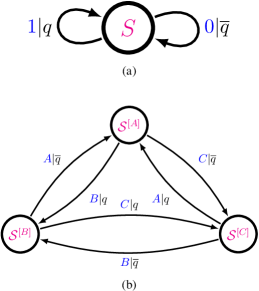
Figure 1: The (a) Hägg-machine and the (b) $ABC$-machine for the IID Process, $q\in[0,1]$. When $q=1$, the IID process generates a string of $1$s, which is physically the 3C⁺ stacking structure. Conversely, for $q=0$, the structure corresponds to the 3C^- structure. For $q=0.5$, the MLs are stacked as randomly as possible. Notice that the single state of the Hägg-machine has split into a three-state $ABC$-machine. This trebling of states is a generic feature of expanding mixing Hägg-machines into $ABC$-machines. (From Riechers et al., (2014), used with permission.)

It is useful to consider limiting cases for $q$. When $q=0.5$, the stacking is completely random, subject only to the stacking constraints preventing two adjacent MLs from having the same orientation. As $q\to 1$, adjacent MLs are almost always cyclically related, and the specimen can be thought of as a 3C⁺ crystal with randomly distributed deformation faults Warren (1969) with probability $\bar{q}$. As $q\to 0$, it is also a 3C crystal with randomly distributed deformation faults, except that the MLs are anticyclically related, which we denote as 3C^-. This is summarized in Table 1.

Table 1: The limiting material structures for the IID Process. Key: DF - deformation fault; Ran - completely random stacking.

$q=0$	$q\approx 0$	$q=\bar{q}=\frac{1}{2}$	$\bar{q}\approx 0$	$\bar{q}=0$
3C-	3C-/DF	Ran	3C+/DF	3C+

The TMs in $ABC$-notation are:

$$\begin{array}[]{r@{\mskip\thickmuskip}l}{\mathcal{T}}^{[A]}=\begin{bmatrix}0&0&0\\ \overline{q}&0&0\\ q&0&0\end{bmatrix},\mskip 5.0mu plus 5.0mu\end{array}\begin{array}[]{r@{\mskip\thickmuskip}l}{\mathcal{T}}^{[B]}=\begin{bmatrix}0&q&0\\ 0&0&0\\ 0&\overline{q}&0\end{bmatrix}\mskip 5.0mu plus 5.0mu\end{array}$$

and

$${\mathcal{T}}^{[C]}=\begin{bmatrix}0&0&\overline{q}\\ 0&0&q\\ 0&0&0\end{bmatrix}.$$

The internal state TM then is their sum:

$${\mathcal{T}}=\begin{bmatrix}0&q&\overline{q}\\ \overline{q}&0&q\\ q&\overline{q}&0\end{bmatrix}~{}.$$

The eigenvalues of the $ABC$ TM are

$$\Lambda_{{\mathcal{T}}}=\{1,\,\Omega,\,\Omega^{*}\}~{},$$

where:

$$\Omega\equiv-\frac{1}{2}+i\frac{\sqrt{3}}{2}(4q^{2}-4q+1)^{1/2}$$

and $\Omega^{*}$ is its complex conjugate.

Furthermore, the stationary distribution over states of the $ABC$-machine can be found from $\bra{{\boldsymbol{\pi}}}=\bra{{\boldsymbol{\pi}}}{\mathcal{T}}$ to be:

$$\bra{{\boldsymbol{\pi}}}=\begin{bmatrix}\tfrac{1}{3}&\tfrac{1}{3}&\frac{1}{3}\end{bmatrix}~{}.$$

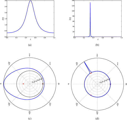
Figure 2: IID Process diffraction patterns for (a) $q=0.5$ and (b) $q=0.99$, as calculated from Eq. (35). Notice that as $q\to 1$, the DP approaches that of a 3C⁺ crystal. For values of $q$ close to but less than 1, the specimen is 3C⁺ with randomly distributed deformation faults. (c) The coronal spectrogram corresponding to $q=0.5$. The enhanced scattering at $\ell=0.5$ in (a) is replaced with the bulge at $\omega=\pi$. There are three eigenvalues for the IID Process, one at $z=1$ and a degenerate pair at $z=-0.5$. (d) The coronal spectrogram corresponding to $q=0.99$. The Bragg-like peak at $\ell=0.33$ in (b) is now represented as a Bragg-like peak at $\omega=2\pi/3.$ Notice how the degenerate eigenvalues in (c) have split and migrated away from the real axis. As they approach the boundary of the unit circle, their presence makes possible Bragg-like reflections in the DP. However, eigenvalues near the unit circle are a necessary, but not sufficient condition for Bragg-like reflections. This is seen in the eigenvalue in the third quadrant that is not accompanied by a Bragg-like reflection.

For $q\in(0,1)$, none of the eigenvalues in $\Lambda_{{\mathcal{T}}}$ besides unity lie on the unit circle of the complex plane, and so there is no possibility of Bragg reflections at non-integer $\ell$. Moreover, since the process is mixing, the Bragg peak at integer $\ell$ is also absent. Thus we need only find the diffuse DP. To calculate the ${\sf{I}}_{{\mathrm{D}}}(\ell)$ as given in Eq. (16), we are only missing $\left(z{\mathbb{I}}-{\mathcal{T}}\right)^{-1}$, which is given by:

$$\left(z{\mathbb{I}}-{\mathcal{T}}\right)^{-1}=\frac{1}{(z-1)(z-\Omega)(z-\Omega^{*})}\times\begin{bmatrix}z^{2}-q\bar{q}&qz+\bar{q}^{2}&\bar{q}z+q^{2}\\ \bar{q}z+q^{2}&z^{2}-q\bar{q}&qz+\bar{q}^{2}\\ qz+\bar{q}^{2}&\bar{q}z+q^{2}&z^{2}-q\bar{q}\end{bmatrix}~{}.$$

Then, with:

$$\bra{{\boldsymbol{\pi}}}{\mathcal{T}}^{[A]}=\begin{bmatrix}\tfrac{1}{3}&0&0\end{bmatrix},$$

we can write

$$\bra{{\boldsymbol{\pi}}}{\mathcal{T}}^{[A]}\left(z{\mathbb{I}}-{\mathcal{T}}\right)^{-1}=\frac{1}{3}\frac{1}{(z-1)(z-\Omega)(z-\Omega^{*})} \times\begin{bmatrix}z^{2}-q\bar{q}&qz+\bar{q}^{2}&\bar{q}z+q^{2}\end{bmatrix},$$

where:

$${\mathcal{T}}^{[{\hat{{\rm{c}}}}(A)]}\ket{{\boldsymbol{1}}}={\mathcal{T}}^{[B]}\ket{{\boldsymbol{1}}}=\begin{bmatrix}q\\ 0\\ \bar{q}\\ \end{bmatrix}$$

and

$${\mathcal{T}}^{[{\hat{{\rm{a}}}}(A)]}\ket{{\boldsymbol{1}}}={\mathcal{T}}^{[C]}\ket{{\boldsymbol{1}}}=\begin{bmatrix}\bar{q}\\ q\\ 0\end{bmatrix}~{}.$$

From Eq. (17), the DP becomes:

$${\sf{I}}_{{\mathrm{D}}}(\ell) =-\frac{6\sqrt{3}}{2}{\mbox{\, \large{$\Re$}}}\left\{\frac{e^{i\pi/6}z\left(q^{2}+\bar{q}z\right)+e^{-i\pi/6}z\left(\bar{q}^{2}+qz\right)}{(z-1)(z-\Omega)(z-\Omega^{*})}\right\}$$ (34)

$$=-2\sqrt{3}{\mbox{\, \large{$\Re$}}}\left\{z\,\frac{e^{i\pi/6}\left(q^{2}+\bar{q}z\right)+e^{-i\pi/6}\left(\bar{q}^{2}+qz\right)}{(z-1)(z^{2}+z+1-3q\bar{q})}\right\}.$$ (35)

For the case of the most random possible stacking in CPSs, where $q=\bar{q}=\frac{1}{2}$, this simplifies to:

$${\sf{I}}_{{\mathrm{D}}}(\ell) =\frac{3/4}{5/4+\cos(2\pi\ell)}.$$ (36)

This result was obtained previously by more elementary means. The results are in agreement. Guinier (1963)

Figure 2 shows DPs and coronal spectrograms for $q=0.5$ and $q=0.99$. Figure 2(a) gives the DP for a maximally disordered stacking process. The spectrum is entirely diffuse with broadband enhancement near $\ell=0.5$. In contrast, the DP for $q=0.99$ in Fig. 2(b) shows a strong Bragg-like reflection at $\ell=0.33$, which we recognize as just the 3C⁺ stacking structure, with a small amount of (as it turns out in this case) deformation faulting. The other two panels in Fig. 2, (c) and (d), are coronal spectrograms giving DPs for these two cases as the radially emanating curve outside the unit circle, but now the three eigenvalues of the total TM are plotted interior to the unit circle. As always, there is a single eigenvalue at $z=1$. In panel (c), the other two degenerate eigenvalues occur at $z=-0.5$, ‘casting a shadow’ on the unit circle in the form of enhanced power at $\omega=\pi$. In panel (d), these eigenvalues split and move away from the real axis closer to the unit circle. In doing so, one casts a more focused shadow in the form of a Bragg-like reflection at $\omega=2\pi/3$. For $q=1$, this eigenvalue finally comes to rest on the unit circle, and the Bragg-like reflection becomes a true Bragg peak, as explored shortly. Note that the other eigenvalue does not give rise to enhanced scattering. We find that having an eigenvalue near the unit circle is necessary to produce enhanced scattering, but the presence of such an eigenvalue does not necessarily guarantee Bragg-like reflections.

IV.1.1 Bragg Peaks from 3C

For the case of $q\in\{0,1\}$, we recover perfect crystalline structure. Although the presence, placement, and magnitude of Bragg peaks are well known from other methods, we show the comprehensive consistency of our method via the example of $q=1$ ($\bar{q}=0$). In this case: $\Lambda_{{\mathcal{T}}}=\{1,\,\Omega,\,\Omega^{*}\}$ with $\Omega=-\frac{1}{2}+i\frac{\sqrt{3}}{2}={\mathrm{e}}^{i2\pi/3}$, so that $\ell_{\Omega}=1/3$ and $\ell_{\Omega^{*}}=2/3$, and the two relevant projection operators reduce to:

$${\mathcal{T}}_{\Omega}=\frac{1}{(\Omega-1)(\Omega-\Omega^{*})}\begin{bmatrix}\Omega^{2}&\Omega&1\\ 1&\Omega^{2}&\Omega\\ \Omega&1&\Omega^{2}\end{bmatrix}$$

and

$${\mathcal{T}}_{\Omega^{*}}=\frac{1}{(\Omega^{*}-1)(\Omega^{*}-\Omega)}\begin{bmatrix}\Omega^{*2}&\Omega^{*}&1\\ 1&\Omega^{*2}&\Omega^{*}\\ \Omega^{*}&1&\Omega^{*2}\end{bmatrix}~{}.$$

From Eq. (26), we have:

$$\Braket{{\mathcal{T}}_{\Omega}^{{\hat{{\rm{c}}}}({\mathcal{A}})}} =\frac{\Omega^{2}}{(\Omega-1)(\Omega-\Omega^{*})}~{},$$

$$\Braket{{\mathcal{T}}_{\Omega}^{{\hat{{\rm{a}}}}({\mathcal{A}})}} =\frac{\Omega}{(\Omega-1)(\Omega-\Omega^{*})}~{},$$

$$\Braket{{\mathcal{T}}_{\Omega^{*}}^{{\hat{{\rm{c}}}}({\mathcal{A}})}} =\frac{\Omega^{*2}}{(\Omega^{*}-1)(\Omega^{*}-\Omega)}~{},$$

and

$$\Braket{{\mathcal{T}}_{\Omega^{*}}^{{\hat{{\rm{a}}}}({\mathcal{A}})}} =\frac{\Omega^{*}}{(\Omega^{*}-1)(\Omega^{*}-\Omega)}~{},$$

which from Eq. (25) yields:

$$\begin{array}[]{r@{\mskip\thickmuskip}l}\Delta_{\Omega}\mskip 5.0mu plus 5.0mu&=1\end{array}\>\>\>{\rm{and}}\>\>\>\begin{array}[]{r@{\mskip\thickmuskip}l}\Delta_{\Omega^{*}}\mskip 5.0mu plus 5.0mu&=0~{}.\end{array}$$

Then, using Eq. (27), the DP’s discrete part becomes:

$${\sf{I}}_{{\mathrm{B}}}(\ell) =\sum_{k=-\infty}^{\infty}\delta(\ell-\tfrac{1}{3}+k)~{},$$

as it ought to be for 3C⁺.

IV.2 Random Growth and Deformation Faults in Layered 3C and 2H CPSs: The RGDF Process

As a simple model of faulting in CPSs, combined random growth and deformation faults are often assumed if the faulting probabilities are believed to be small. However, until now there has not been an analytical expression available for the DP for all values of the faulting parameters, and we derive such an expression here.

The HMM for the Random Growth and Deformation Faults (RGDF) process was first proposed by Estevez-Rams et al. (2008) and the Hägg-machine is shown in Fig. 3. The process has two parameters, $\alpha\in[0,1]$ and $\beta\in[0,1]$, that (at least for small values) are interpreted as the probability of deformation and growth faults, respectively. The stacking process, however, is described best on its own terms—in terms of the HMM, which captures the causal architecture of the stacking for all parameter values.

Figure 3: Hägg-machine for the RGDF Process as proposed by Estevez et al. (2008). This two-state machine has two parameters, $\alpha\in[0,1]$ and $\beta\in[0,1]$, the probability of deformation and growth faults in CPSs, respectively. (From Riechers et al. (2014), used with permission.)

It is instructive to consider limiting values of $\alpha$ and $\beta$. For $\alpha=\beta=0$, the stacking structure is simply 3C. The machine splits into two distinct machines: each machine has one state with a single self-state transition, corresponding to the 3C⁺ stacking structure and the other to 3C^- stacking structure. The 2H stacking structure occurs when $\alpha=\bar{\beta}=0$. Typically growth faults are introduced as $\beta$ strays from these limiting values, and deformation faults appear when $\alpha$ becomes small but nonvanishing. When $\alpha=1/2$, the stacking becomes completely random, regardless of the value of $\beta$. This is summarized in Table 2.

Table 2: The limiting material structures for the RGDF Process. Key: GF - growth fault; DF - deformation fault; Ran - completely random stacking.

	$\beta=0$	$\beta\approx 0$	$\beta=\bar{\beta}=1/2$	$\bar{\beta}\approx 0$	$\bar{\beta}=0$
$\alpha=0$	3C	3C/GF	Ran	2H/GF	2H
$\alpha\approx 0$	3C/DF	3C/DF,GF	Ran	2H/DF,GF	2H/DF
$\alpha=\frac{1}{2}$	Ran	Ran	Ran	Ran	Ran

The RGDF Hägg-machine’s TMs are:

$$\begin{array}[]{r@{\mskip\thickmuskip}l}{\sf{T}}^{[0]}\mskip 5.0mu plus 5.0mu&=\begin{bmatrix}\alpha\overline{\beta}&\overline{\alpha}\beta\\ \alpha\beta&\overline{\alpha}\overline{\beta}\end{bmatrix}\end{array}{\rm{and}}\begin{array}[]{r@{\mskip\thickmuskip}l}{\sf{T}}^{[1]}\mskip 5.0mu plus 5.0mu&=\begin{bmatrix}\overline{\alpha}\overline{\beta}&\alpha\beta\\ \overline{\alpha}\beta&\alpha\overline{\beta}\end{bmatrix}.\end{array}$$

The Hägg-machine is nonmixing only for the parameter settings $\beta=1$ and $\alpha\in\{0,1\}$, giving rise to 2H crystal structure.

From the Hägg-machine, we obtain the corresponding TMs of the $ABC$-machine for $\alpha,\beta\in(0,1)$: Riechers et al. (2014)

$${\mathcal{T}}^{[A]} =\begin{bmatrix}0&0&0&0&0&0\\ \alpha\overline{\beta}&0&0&\overline{\alpha}\beta&0&0\\ \overline{\alpha}\overline{\beta}&0&0&\alpha\beta&0&0\\ 0&0&0&0&0&0\\ \alpha\beta&0&0&\overline{\alpha}\overline{\beta}&0&0\\ \overline{\alpha}\beta&0&0&\alpha\overline{\beta}&0&0\\ \end{bmatrix},$$

$$\vspace{.05in}{\mathcal{T}}^{[B]} =\begin{bmatrix}0&\overline{\alpha}\overline{\beta}&0&0&\alpha\beta&0\\ 0&0&0&0&0&0\\ 0&\alpha\overline{\beta}&0&0&\overline{\alpha}\beta&0\\ 0&\overline{\alpha}\beta&0&0&\alpha\overline{\beta}&0\\ 0&0&0&0&0&0\\ 0&\alpha\beta&0&0&\overline{\alpha}\overline{\beta}&0\\ \end{bmatrix},$$

and

$${\mathcal{T}}^{[C]} =\begin{bmatrix}0&0&\alpha\overline{\beta}&0&0&\overline{\alpha}\beta\\ 0&0&\overline{\alpha}\overline{\beta}&0&0&\alpha\beta\\ 0&0&0&0&0&0\\ 0&0&\alpha\beta&0&0&\overline{\alpha}\overline{\beta}\\ 0&0&\overline{\alpha}\beta&0&0&\alpha\overline{\beta}\\ 0&0&0&0&0&0\\ \end{bmatrix},$$

and the orientation-agnostic state-to-state TM:

$${\mathcal{T}} ={\mathcal{T}}^{[A]}+{\mathcal{T}}^{[B]}+{\mathcal{T}}^{[C]}.$$

Explicitly, we have:

$${\mathcal{T}} =\begin{bmatrix}0&\overline{\alpha}\overline{\beta}&\alpha\overline{\beta}&0&\alpha\beta&\overline{\alpha}\beta\\ \alpha\overline{\beta}&0&\overline{\alpha}\overline{\beta}&\overline{\alpha}\beta&0&\alpha\beta\\ \overline{\alpha}\overline{\beta}&\alpha\overline{\beta}&0&\alpha\beta&\overline{\alpha}\beta&0\\ 0&\overline{\alpha}\beta&\alpha\beta&0&\alpha\overline{\beta}&\overline{\alpha}\overline{\beta}\\ \alpha\beta&0&\overline{\alpha}\beta&\overline{\alpha}\overline{\beta}&0&\alpha\overline{\beta}\\ \overline{\alpha}\beta&\alpha\beta&0&\alpha\overline{\beta}&\overline{\alpha}\overline{\beta}&0\\ \end{bmatrix}.$$

${\mathcal{T}}$’s eigenvalues satisfy det$({\mathcal{T}}-\lambda{\mathbb{I}})=0$, from which we obtain the eigenvalues: Riechers et al. (2014)

$$\Lambda_{{\mathcal{T}}} =\left\{1,\,1-2\beta,\,-\tfrac{1}{2}(1-\beta)\pm\tfrac{1}{2}\sqrt{\sigma}\right\},$$ (37)

with

$$\sigma \equiv 4\beta^{2}-3\overline{\beta}^{2}+12\alpha\overline{\alpha}(\overline{\beta}-\beta)$$ (38)

$$=-3+12\alpha+6\beta-12\alpha^{2}+\beta^{2}-24\alpha\beta+24\alpha^{2}\beta.$$ (39)

Except for measure-zero submanifolds along which the eigenvalues become extra degenerate, throughout the parameter range the eigenvalues’ algebraic multiplicities are: $a_{1}=1$, $a_{1-2\beta}=1$, $a_{-\tfrac{1}{2}(1-\beta+\sqrt{\sigma})}=2$, and $a_{-\tfrac{1}{2}(1-\beta-\sqrt{\sigma})}=2$. Moreover, the index of all eigenvalues is 1 except along $\sigma=0$. Hence, due to their qualitative difference, we treat the cases of $\sigma=0$ and $\sigma\neq 0$ separately.

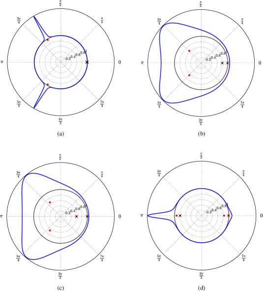
Figure 4: Coronal spectrograms showing the DP and eigenvalues for the RGDF Process: (a) $\alpha=0.01$, $\beta=0.01$; (b) $\alpha=0.2$, $\beta=0.1$; (c) $\alpha=0.1$, $\beta=0.2$; and (d) $\alpha=0.01$, $\beta=0.9$. Note how the eigenvalues organize the DP: as the eigenvalues approach the unit circle, the DP becomes enhanced. Also, note that nowhere is there enhanced scattering without an underlying eigenvalue of the TM driving it.

IV.2.1 $\sigma=0$:

Riechers et al. Riechers et al. (2014) found that:

$$\Braket{{\mathcal{T}}_{1}^{{\hat{{\rm{c}}}}({\mathcal{A}})}}=\Braket{{\mathcal{T}}_{1}^{{\hat{{\rm{a}}}}({\mathcal{A}})}} =\tfrac{1}{3}~{},$$

$$\Braket{{\mathcal{T}}_{1-2\beta}^{{\hat{{\rm{c}}}}({\mathcal{A}})}}=\Braket{{\mathcal{T}}_{1-2\beta}^{{\hat{{\rm{a}}}}({\mathcal{A}})}} =0~{},$$

$$\Braket{{\mathcal{T}}_{-\overline{\beta}/2}^{{\hat{{\rm{c}}}}({\mathcal{A}})}}=\Braket{{\mathcal{T}}_{-\overline{\beta}/2}^{{\hat{{\rm{a}}}}({\mathcal{A}})}} =\tfrac{1}{6}~{},$$

and

$$\Braket{{\mathcal{T}}_{-\overline{\beta}/2,1}^{{\hat{{\rm{c}}}}({\mathcal{A}})}}=\Braket{{\mathcal{T}}_{-\overline{\beta}/2,1}^{{\hat{{\rm{a}}}}({\mathcal{A}})}} =-\tfrac{1}{12}\beta\overline{\beta}~{},$$

for the case of $\sigma=0$. According to Eq. (33), the DP for $\sigma=0$ is thus:

$${\sf{I}}_{{\mathrm{D}}}(\ell) =-6{\mbox{\, \large{$\Re$}}}\left\{\sum_{\lambda\in\Lambda_{{\mathcal{T}}}}\sum_{m=0}^{\nu_{\lambda}-1}\frac{\Braket{{\mathcal{T}}_{\lambda,m}^{{\hat{{\rm{c}}}}({\mathcal{A}})}}}{(z-\lambda)^{m+1}}\right\}$$

$$=-6{\mbox{\, \large{$\Re$}}}\left\{\frac{\Braket{{\mathcal{T}}_{1}^{{\hat{{\rm{c}}}}({\mathcal{A}})}}}{z-1}+\frac{\Braket{{\mathcal{T}}_{-\bar{\beta}/2}^{{\hat{{\rm{c}}}}({\mathcal{A}})}}}{z+\bar{\beta}/2}+\frac{\Braket{{\mathcal{T}}_{-\bar{\beta}/2,1}^{{\hat{{\rm{c}}}}({\mathcal{A}})}}}{\left(z+\bar{\beta}/2\right)^{2}}\right\}$$

$$={\mbox{\, \large{$\Re$}}}\left\{-\frac{2}{z-1}-\frac{1}{z+\bar{\beta}/2}+\frac{\beta\bar{\beta}/2}{\left(z+\bar{\beta}/2\right)^{2}}\right\}$$

$$=1-{\mbox{\, \large{$\Re$}}}\left\{\frac{z+\bar{\beta}^{2}/2}{\left(z+\bar{\beta}/2\right)^{2}}\right\}~{}.$$ (40)

IV.2.2 $\sigma\neq 0$:

Riechers et al. Riechers et al. (2014) also found that:

$$\Braket{{\mathcal{T}}_{1}^{{\hat{{\rm{c}}}}({\mathcal{A}})}} =\Braket{{\mathcal{T}}_{1}^{{\hat{{\rm{a}}}}({\mathcal{A}})}}=\tfrac{1}{3}~{},$$

$$\Braket{{\mathcal{T}}_{1-2\beta}^{{\hat{{\rm{c}}}}({\mathcal{A}})}} =\Braket{{\mathcal{T}}_{1-2\beta}^{{\hat{{\rm{a}}}}({\mathcal{A}})}}=0~{},$$

$$\Braket{T_{\frac{-\overline{\beta}+\sqrt{\sigma}}{2}}^{{\hat{{\rm{c}}}}({\mathcal{A}})}} =\Braket{T_{\frac{-\overline{\beta}+\sqrt{\sigma}}{2}}^{{\hat{{\rm{a}}}}({\mathcal{A}})}}$$

$$=-\tfrac{1}{12}\left(1-\frac{\beta}{\sqrt{\sigma}}\right)\left(\sqrt{\sigma}-\overline{\beta}\right)~{},$$

and

$$\Braket{T_{\frac{-\overline{\beta}-\sqrt{\sigma}}{2}}^{{\hat{{\rm{c}}}}({\mathcal{A}})}} =\Braket{T_{\frac{-\overline{\beta}-\sqrt{\sigma}}{2}}^{{\hat{{\rm{a}}}}({\mathcal{A}})}}$$

$$=\tfrac{1}{12}\left(1+\frac{\beta}{\sqrt{\sigma}}\right)\left(\sqrt{\sigma}+\overline{\beta}\right)~{},$$

for $\sigma\neq 0$. According to Eq. (33), the DP for $\sigma\neq 0$ is:

$${\sf{I}}_{{\mathrm{D}}}(\ell) =-6{\mbox{\, \large{$\Re$}}}\left\{\sum_{\lambda\in\Lambda_{{\mathcal{T}}}}\frac{\Braket{{\mathcal{T}}_{\lambda}^{{\hat{{\rm{c}}}}({\mathcal{A}})}}}{z-\lambda}\right\}$$

$$=-6{\mbox{\, \large{$\Re$}}}\left\{\frac{\Braket{{\mathcal{T}}_{1}^{{\hat{{\rm{c}}}}({\mathcal{A}})}}}{z-1}+\frac{\Braket{{\mathcal{T}}_{\frac{-\overline{\beta}+\sqrt{\sigma}}{2}}^{{\hat{{\rm{c}}}}({\mathcal{A}})}}}{z-\frac{\sqrt{\sigma}-\overline{\beta}}{2}}+\frac{\Braket{{\mathcal{T}}_{\frac{-\overline{\beta}-\sqrt{\sigma}}{2}}^{{\hat{{\rm{c}}}}({\mathcal{A}})}}}{z+\frac{\sqrt{\sigma}+\overline{\beta}}{2}}\right\}$$

$$=1+\tfrac{1}{2}{\mbox{\, \large{$\Re$}}}\left\{\frac{1-\beta/\sqrt{\sigma}}{\frac{z}{\sqrt{\sigma}-\bar{\beta}}-\frac{1}{2}}-\frac{1+\beta/\sqrt{\sigma}}{\frac{z}{\sqrt{\sigma}+\bar{\beta}}+\frac{1}{2}}\right\}~{}.$$ (41)

Figure 4 gives several coronal spectrograms for various values of the parameters $\alpha$ and $\beta$. It is instructive to examine the influence of the TM’s eigenvalues on the placement and intensity of the Bragg-like reflections. In panel (a) there are two strong reflections, one each at $\omega=2\pi/3$ and $4\pi/3$, signaling a twinned 3C structure, when the faulting parameters are set to $\alpha=\beta=0.01$. Each is accompanied by an eigenvalue close to the surface of the unit circle. As the disorder is increased, see panels (b) and (c), TM eigenvalues retreat toward the center of the unit circle and the two strong reflections become diffuse. However, in the final panel (d), the faulting parameters ($\alpha=0.01$, $\beta=0.9$) are set such that the material has apparently undergone a phase transition from prominently 3C stacking structure to prominently 2H stacking structure. Indeed, the eigenvalues have coalesced through the critical point of $\sigma=0$ (as $\sigma$ changes from negative to positive) and emerge on the other side of the phase transition mutually scattered along the real axis and approaching the edge of the unit circle, giving rise to the 2H-like protrusions in the DP. This demonstrates again how the eigenvalues orchestrate the placement and intensity of the Bragg-like peaks.

IV.3 Shockley–Frank Stacking Faults in 6H-SiC: The SFSF Process

SiC has been the intense focus of both experimental and theoretical investigations for some time due to its promise as a material suitable for next-generation electronic devices. However, it is known that SiC can have many different stacking configurations—some ordered and some disorderedSebastian and Krishna (1994)—and these different stacking configurations can profoundly affect material properties. Despite considerable effort to grow commercial SiC wafers that are purely crystalline—i.e., that have no stacking defects—reliable techniques have not yet been developed. It is therefore important to better understand and characterize the nature of the defects in order to better control them.

Recently, Sun et al. Sun et al. (2012) reported experiments on 6H-SiC that used a combination of low temperature photoluminescence and high resolution transmission electron microscopy (HRTEM). One of the more common crystalline forms of SiC, the 6H stacking structure is simply the sequence …ABCACBA …, or in terms of the Hägg-notation, …111000 …. The most common stacking fault in 6H-SiC identified by HRTEM can be explained as the result of one extrinsic Frank stacking fault coupled with one Shockley stacking fault. Hirth and Lothe (1968) Physically, the resultant stacking structure corresponds to the insertion of an additional SiC ML so that one has instead …$11000\underline{0}111000$ …, where the underlined spin is the inserted ML.

Inspired by these findings, we suggest a simple HMM for the Shockley–Frank stacking fault (SFSF) process that replicates this structure, and this is shown in Fig. 5. Our motivation here is largely pedagogical, and certainly more detailed experiments are required to confidently propose a structure, but this HMM reproduces at least qualitatively the observed structure. The model has a single parameter $\gamma\in[0,1]$. As before, it is instructive to consider limiting cases of $\gamma$. For $\gamma=0$, we have the pure 6H structure and, for small $\gamma$, Shockley–Frank defects are introduced into this stacking structure. As $\gamma\to 1$, the structure transitions into a twinned 3C crystal. However, unlike the previous example, this twinning is not random. Instead, the architecture of the machine requires that at least three 0s or 1s must be seen before there is a possibility of reversing the chirality, i.e., before there is twinning. These limiting cases are summarized in Table 3.

Table 3: Limiting material structures for the SFSF Process. Key: SF - Shockley–Frank fault; NGF - nonrandom growth fault.

$\gamma=0$	$\gamma\approx 0$	$\bar{\gamma}\approx 0$	$\bar{\gamma}=0$
6H	6H/SF	3C/NGF	3C

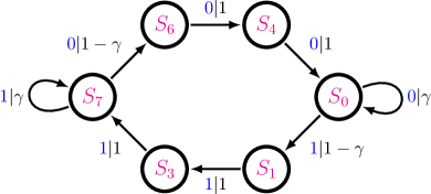
Figure 5: Hägg-machine for the SFSF Process. There is one faulting parameter $\gamma\in[0,1]$ and three SSCs or, equivalently, three CSCs, as this machine is also an $\epsilon$-machine. The three SSCs are [$\sf{S}_{7}$], [$\sf{S}_{0}]$ and [$\sf{S}_{7}\sf{S}_{6}\sf{S}_{4}\sf{S}_{0}\sf{S}_{1}\sf{S}_{3}$]. The latter we recognize as the 6H structure if $\gamma=0$. For large values of $\gamma$—i.e., as $\gamma\to 1$—this process approaches a twinned 3C structure, although the faulting is not random. The causal-state architecture prevents the occurrence of domains of size-three or less. (From Riechers et al. Riechers et al. (2014) Used with permission.)

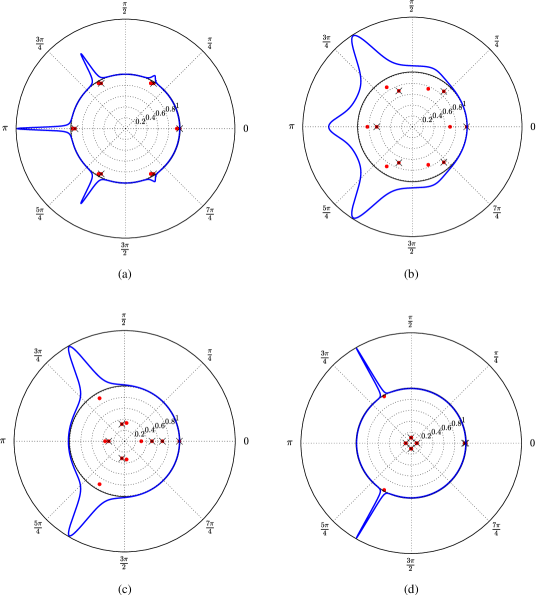
Figure 6: Coronal spectrograms showing the evolution of the DP and its eigenvalues for the SFSF Process. (a) $\gamma=0.1$, (b) $\gamma=0.5$, (c) $\gamma=0.9$, and (d) $\gamma=0.99$. In (a) the faulting is weak and the DP has the six degraded Bragg-like reflections characteristic of the 6H stacking structure. In (b), the faulting is more severe, with the concomitant erosion of the Bragg-like reflections, especially for $\omega=\pi$. In panel (c) the 6H character has been eliminated, and the Bragg-like peaks at $\omega=2\pi/3$ and $4\pi/3$ are now associated with a twinned 3C stacking structure. In panel (d), the Bragg-like reflections sharpen as the probability of short 3C sequences stacking sequences decreases.

For $\gamma\in(0,1)$ the Hägg-machine is mixing and we proceed with this case. By inspection, we write down the two 6-by-6 TMs of the Hägg-machine as:

$${\sf{T}}^{[0]} =\begin{bmatrix}\gamma&0&0&0&0&0\\ 0&0&0&0&0&0\\ 0&0&0&0&0&0\\ 0&0&0&0&\overline{\gamma}&0\\ 0&0&0&0&0&1\\ 1&0&0&0&0&0\\ \end{bmatrix}$$

and:

$${\sf{T}}^{[1]} =\begin{bmatrix}0&\overline{\gamma}&0&0&0&0\\ 0&0&1&0&0&0\\ 0&0&0&1&0&0\\ 0&0&0&\gamma&0&0\\ 0&0&0&0&0&0\\ 0&0&0&0&0&0\\ \end{bmatrix},$$

where the states are ordered $\sf{S}_{0}$, $\sf{S}_{1}$, $\sf{S}_{3}$, $\sf{S}_{7}$, $\sf{S}_{6}$, and $\sf{S}_{4}$. The internal state TM is their sum:

$${\sf{T}} =\begin{bmatrix}\gamma&\overline{\gamma}&0&0&0&0\\ 0&0&1&0&0&0\\ 0&0&0&1&0&0\\ 0&0&0&\gamma&\overline{\gamma}&0\\ 0&0&0&0&0&1\\ 1&0&0&0&0&0\\ \end{bmatrix}.$$

Since the six-state Hägg-machine generates an ($3\times 6=$) eighteen-state $ABC$-machine, we do not explicitly write out its TMs. Nevertheless, it is straightforward to expand the Hägg-machine to the $ABC$-machine via the rote expansion method. Riechers et al. (2014) It is also straightforward to apply Eq. (17) to obtain the DP as a function of the faulting parameter $\gamma$. To use Eq. (17), note that the stationary distribution over the $ABC$-machine can be obtained from Eq. (42) with:

$$\bra{{\boldsymbol{\pi}}_{\textrm{H}}} =\tfrac{1}{6-4\gamma}\begin{bmatrix}1&\overline{\gamma}&\overline{\gamma}&1&\overline{\gamma}&\overline{\gamma}\end{bmatrix}$$

as the stationary distribution over the Hägg-machine.

The eigenvalues of the Hägg TM can be obtained as the solutions of $\det({\sf{T}}-\lambda{\mathbb{I}})=(\lambda-\gamma)^{2}\lambda^{4}-\overline{\gamma}^{2}=0$. These include $1$, $-\tfrac{1}{2}\overline{\gamma}\pm\sqrt{\gamma^{2}+2\gamma-3}$, and three other eigenvalues involving cube roots.

The eigenvalues of the $ABC$ TM are obtained similarly as the solutions of $\det({\mathcal{T}}-\lambda{\mathbb{I}})=0$. Note that $\Lambda_{{\mathcal{T}}}$ inherits $\Lambda_{{\sf{T}}}$ as the backbone for its more complex structure, just as $\Lambda_{{\sf{T}}}\subseteq\Lambda_{{\mathcal{T}}}$ for all of our previous examples. The eigenvalues in $\Lambda_{{\mathcal{T}}}$ are, of course, those most directly responsible for the structure of the CFs. Since the $ABC$-machine has eighteen states, there are eighteen eigenvalues contributing to the behavior of the DP; although several eigenvalues are degenerate. Hence, the SFSF Process is capable of a richer DP than the previous two examples.

The coronal spectrograms for the SFSF Process are shown for several example values of $\gamma$ in Fig. 6. Over the range of $\gamma$ values the stacking structure changes from a nearly perfect 6H crystal through a disordered phase finally becoming a twinned 3C structure. Most notable in Fig. 6 is how the eigenvalues of the total TM dictate the placement of the Bragg-like reflections. Phrased alternatively, the Bragg-like reflections appear to literally track the movement of the eigenvalues as they evolve during transformation.

V Conclusions

We showed how the DP for an arbitrary HMM stacking process is calculated either analytically or to a high degree of numerical certainty directly without restriction to finite Markov order and without needing finite samples of the stacking sequence. Along the way, we uncovered a remarkably simple relationship between the DP and the HMM. The former is given by straightforward, standard matrix manipulations of the latter. Critically, in the case of an infinite number of MLs, this relationship does not involve powers of the TM.

The connection yields important insights. (i) The number of Bragg and Bragg-like reflections in the DP is limited by the size of the TMs that define the HMM. Thus, knowing only the number of machine states reveals the maximum possible number of Bragg and Bragg-like reflections. (ii) As a corollary, given a DP, the number of Bragg and Bragg-like reflections puts a minimum on the number of HMM states. For the problem of inferring the HMM from experimental DPs, this gives powerful clues about the HMM (and so internal mechanism) architecture. (iii) The eigenvalues within the unit circle organize the diffuse Bragg-like reflections. Only TM eigenvalues on the unit circle correspond to those $\ell$-values that potentially can result in true Bragg peaks. (iv) The expansion of the Hägg-machine into the $ABC$-machine, necessary for the appropriate matrix manipulations, showed that there are two kinds of machines and, hence, two kinds of stacking process important in CPSs: mixing and nonmixing processes. In addition to the calculational shortcuts given by the former, mixing machines ensure that there are no true Bragg reflections at integer-$\ell$. (v) Conversely, the presence of Bragg peaks at integer-$\ell$ is an unmistakable sign that a stacking process is nonmixing. Again, this puts important constraints on the HMM state architecture, useful for the problem of inverting the DP to find the HMM. (vi) For mixing processes, the ML probabilities must all be one-third, i.e., $\Pr(A)=\Pr(B)=\Pr(C)=1/3$.

New in the theory is the introduction of coronal spectrograms, a convenient way to visualize the interplay between a frequency-domain functional of a process and the eigenvalues of the process’s TMs. In our case, the frequency-domain functional was the DP: the power spectrum of the sequence of ML structure factors. In each of the examples, the movement of the eigenvalues (as the HMM parameters change) were echoed by movement of their ‘shadow’—the Bragg-like peaks in the power spectrum. While this technique was explored in the context of DPs from layered materials, this visualization tool is by no means confined to DPs or layered materials. We suspect that in other areas where power spectra and HMMs are studied, this technique will become a useful analysis tool.

There are several important research directions to follow in further refining and extending the theory and developing applications. (i) While specialized to CPSs here, the basic techniques extend to other stacking geometries and other materials, including the gamut of technologically cutting-edge heterostructures of stacked 2D materials. (ii) With the ability to analytically calculate DPs and CFs Riechers et al. (2014) from arbitrary HMMs, the number of physical and information- and computation-theoretic quantities amenable to such a treatment continues to expand. Statistical complexity, the Shannon entropy rate, and memory length have long been calculable from the $\epsilon$-machine, Crutchfield and Young (1989); Varn et al. (2007, 2013a, 2013b) but recently the excess entropy, transient information, and synchronization time have also been shown to be exactly calculable from the $\epsilon$-machine. Crutchfield et al. (2013); Riechers and Crutchfield (2014) This portends well that additional quantities, especially those of physical import such as band structure in chaotic crystals, may also be treatable with exact methods. (iii) Improved calculational techniques raise the possibility of improved inference methods, so that more kinds of stacking process may be discovered from DPs. An important research direction then is to incorporate these improved methods into more flexible, more sensitive inference algorithms.

Finally, the spectral methods pursued here increase the tools available to chaotic crystallography for the discovery, description, and categorization of both ordered and disordered (chaotic) crystals. With these tools in hand, we will more readily identify key features of the hidden structures responsible for novel physical properties of materials.

Appendix A Hägg-to-$ABC$ Machine Translation

If ${\sf M}_{\rm H}$ is the number of states in the Hägg-machine and $M$ is the number of states in the $ABC$-machine, then $M=3{\sf M}_{\rm H}$ for mixing Hägg-machines. Let the $i^{\rm{th}}$ state of the Hägg-machine split into the ${\left(3i-2\right)}^{\rm{th}}$ through the ${\left(3i\right)}^{\rm{th}}$ states of the corresponding $ABC$-machine. Then, each labeled-edge transition from the $i^{\rm{th}}$ to the $j^{\rm{th}}$ states of the Hägg-machine maps into a 3-by-3 submatrix for each of the three labeled TMs of the $ABC$-machine as:

$$\left\{{\sf{T}}_{ij}^{[0]}\right\}\xRightarrow{\text{H\"{a}gg\ to }ABC}\left\{{\mathcal{T}}_{3i-1,3j-2}^{[A]},\text{ }{\mathcal{T}}_{3i,3j-1}^{[B]},\text{ }{\mathcal{T}}_{3i-2,3j}^{[C]}\right\}$$

and

$$\left\{{\sf{T}}_{ij}^{[1]}\right\}\xRightarrow{\text{H\"{a}gg\ to }ABC}\left\{{\mathcal{T}}_{3i,3j-2}^{[A]},\text{ }{\mathcal{T}}_{3i-2,3j-1}^{[B]},\text{ }{\mathcal{T}}_{3i-1,3j}^{[C]}\right\}.$$

For nonmixing Hägg-machines, the above algorithm creates three disconnected $ABC$-machines, of which only one need be retained.

Furthermore, for mixing Hägg-machines, the probability from the stationary distribution over their states maps to a triplet of probabilities for the stationary distribution over the $ABC$-machine states:

$$\left\{{p_{i}^{\text{H}}}\right\}\xRightarrow{\text{H\"{a}gg\ to }ABC}\left\{3p_{3i-2},\text{ }3p_{3i-1},\text{ }3p_{3i}\right\}~{}.$$ (42)

A thorough exposition of these procedures is given by Riechers et al.. Riechers et al. (2014)

References

- Hirth and Lothe (1968) J. P. Hirth and J. Lothe, Theory of Dislocations, 2nd ed. (McGraw-Hill, New York, 1968).
- Caroff et al. (2011) P. Caroff, J. Bolinsson, and J. Johansson, IEEE Journal of Selected Topics in Quantum Electronics 17, 829 (2011).
- Geim and Grigorieva (2013) A. K. Geim and I. V. Grigorieva, Nature 499, 419 (2013).
- Pan et al. (2009) D. Pan, S. Wang, B. Zhao, M. Wu, H. Zhang, Y. Wang, and Z. Jiao, Chemistry of Materials 21, 3136 (2009).
- Seebauer and Noh (2010) E. G. Seebauer and K. W. Noh, Mater. Sci. Eng. R 70, 151 (2010).
- A. L. Mackay (1986) A. L. Mackay, Computers & Mathematics with Applications B12, 21 (1986).
- Cartwright and Mackay (2012) J. H. E. Cartwright and A. L. Mackay, Phil. Trans. R. Soc. A 370, 2807 (2012).
- Varn and Crutchfield (2014) D. P. Varn and J. P. Crutchfield, Santa Fe Institute Working Paper 14-09-036 (2014), arXiv:1409.5930 [cond-mat.stat-mech] .
- Crutchfield (2012) J. P. Crutchfield, Nature Physics 8, 17 (2012).
- Shalizi and Crutchfield (2001) C. R. Shalizi and J. P. Crutchfield, J. Stat. Phys. 104, 817 (2001).
- Cover and Thomas (2006) T. M. Cover and J. A. Thomas, Elements of Information Theory, 2nd ed. (John Wiley & Sons, Hoboken, 2006).
- Paz (1971) A. Paz, Introduction to Probabilistic Automata (Academic Press, New York, 1971).
- Hopcroft and Ullman (1979) J. E. Hopcroft and J. D. Ullman, Introduction to Automata Theory, Languages, and Computation (Addison-Wesley, Reading, 1979).
- Strogatz (2001) S. H. Strogatz, Nonlinear Dynamics and Chaos: With Applications to Physics, Biology, Chemistry, and Engineering (Westview Press, 2001).
- Feldman (2012) D. P. Feldman, Chaos and Fractals: An Elementary Introduction (Oxford University Press, Oxford, 2012).
- Palmer et al. (2000) A. J. Palmer, C. W. Fairall, and W. A. Brewer, IEEE Trans. Geosci. Remote Sens. 38, 2056 (2000).
- Clarke et al. (2003) R. W. Clarke, M. P. Freeman, and N. W. Watkins, Phys. Rev. E 67, 016203 (2003).
- Kelly et al. (2012) D. Kelly, M. Dillingham, A. Hudson, and K. Wiesner, Public Library of Science One 7, e29703 (2012).
- Price (1983) G. D. Price, Phys. Chem. Minerals 10, 77 (1983).
- Ferraris et al. (2008) G. Ferraris, E. Makovicky, and S. Merlino, Crystallography of Modular Materials, Vol. 15 (Oxford University Press, 2008).
- Varn et al. (2002) D. P. Varn, G. S. Canright, and J. P. Crutchfield, Phys. Rev. B 66, 174110 (2002).
- Riechers et al. (2014) P. M. Riechers, D. P. Varn, and J. P. Crutchfield, Santa Fe Institute Working Paper 2014-08-026 (2014), arXiv:1407.7159 [cond-mat.mtrl-sci] .
- Hendricks and Teller (1942) S. Hendricks and E. Teller, J. Chem. Phys. 10, 147 (1942).
- Wilson (1942) A. J. C. Wilson, Proc. R. Soc. Ser. A 180, 277 (1942).
- Kakinoki and Komura (1965) J. Kakinoki and Y. Komura, Acta Crystallogr. 19, 137 (1965).
- Holloway and Klamkin (1969) H. Holloway and M. S. Klamkin, J. Appl. Phys. 40, 1681 (1969).
- Holloway (1969) H. Holloway, J. Appl. Phys. 40, 4313 (1969).
- Pandey et al. (1980a) D. Pandey, S. Lele, and P. Krishna, Proc. R. Soc. London Ser. A 369, 435 (1980a).
- Pandey et al. (1980b) D. Pandey, S. Lele, and P. Krishna, Proc. R. Soc. London Ser. A 369, 451 (1980b).
- Pandey et al. (1980c) D. Pandey, S. Lele, and P. Krishna, Proc. R. Soc. London Ser. A 369, 463 (1980c).
- Sebastian and Krishna (1994) M. T. Sebastian and P. Krishna, Random, Non-Random and Periodic Faulting in Crystals (Gordon and Breach, The Netherlands, 1994).
- Gosk (2001) J. B. Gosk, Crys. Res. Tech. 36, 197 (2001).
- Kopp et al. (2012) V. S. Kopp, V. M. Kaganer, J. Schwarzkopf, F. Waidick, T. Remmele, A. Kwasniewski, and M. Schmidbauer, Acta Crystallogr. Sec. A 68, 148 (2012).
- Berliner and Werner (1986) R. Berliner and S. Werner, Phys. Rev. B 34, 3586 (1986).
- Kantz and Schreiber (2004) H. Kantz and T. Schreiber, Nonlinear Time Series Analysis, 2nd ed. (Cambridge University Press, Cambridge, 2004).
- Nikolin and Babkevich (1989) B. I. Nikolin and A. Y. Babkevich, Acta Crystallogr. Sec. A 45, 797 (1989).
- Varn (2001) D. P. Varn, Language Extraction from ZnS, Ph.D. thesis, University of Tennessee, Knoxville (2001).
- Varn et al. (2013a) D. P. Varn, G. S. Canright, and J. P. Crutchfield, Acta Crystallogr. Sec. A 69, 197 (2013a).
- Keen and McGreevy (1990) D. A. Keen and R. L. McGreevy, Nature 344, 423 (1990).
- Michels-Clark et al. (2013) T. M. Michels-Clark, V. E. Lynch, C. M. Hoffmann, J. Hauser, T. Weber, R. Harrison, and H. B. Bürgi, J. Appl. Crystallogr. 46, 1616 (2013).
- Johnson et al. (2010) B. D. Johnson, J. P. Crutchield, C. J. Ellison, and C. S. McTague, Santa Fe Institute Working Paper 10-11-027 (2010), arXiv:1011.0036v3 [cs.FL] .
- Strelioff and Crutchfield (2014) C. C. Strelioff and J. P. Crutchfield, Phys. Rev. E 89, 042119 (2014).
- Badii and Politi (1997) R. Badii and A. Politi, Complexity: Hierarchical Structures and Scaling in Physics, Cambridge Nonlinear Science Series, Vol. 6 (Cambridge University Press, 1997).
- Varn and Crutchfield (2004) D. P. Varn and J. P. Crutchfield, Phys. Lett. A 324, 299 (2004).
- Baake and Grimm (2012) M. Baake and U. Grimm, Chem. Soc. Rev 41, 6821–6843 (2012).
- Ashcroft and Mermin (1976) N. W. Ashcroft and N. D. Mermin, Solid State Physics (Saunders College Publishing, New York, 1976).
- Ortiz et al. (2013) A. L. Ortiz, F. Sánchez-Bajo, F. L. Cumbrera, and F. Guiberteau, J. Appl. Crystallogr. 46, 242 (2013).
- Note (1) For power spectra of finite-length sequences, there is no clear distinction among these features.
- Axel and Terauchi (1991) F. Axel and H. Terauchi, Phys. Rev. Lett. 66, 2223 (1991).
- Kabra and Pandey (1988) V. K. Kabra and D. Pandey, Phys. Rev. Lett. 61, 1493 (1988).
- Yi and Canright (1996) J. Yi and G. S. Canright, Phys. Rev. B 53, 5198 (1996).
- Varn and Canright (2001) D. P. Varn and G. S. Canright, Acta Crystallogr. Sec. A 57, 4 (2001).
- Note (2) As previously done, Varn et al. (2013a) we divide out those factors associated with experimental corrections to the observed DP, as well as the total number of MLs, so that has only those contributions arising from the stacking structure itself. Here and elsewhere, we refer to simply as the DP.
- Estevez-Rams et al. (2003) E. Estevez-Rams, B. Aragon-Fernandez, H. Fuess, and A. Penton-Madrigal, Phys. Rev. B 68, 064111 (2003).
- Note (3) It may seem that specializing to such a specific expression for the DP at this stage limits the applicability of the approach. While the development here is restricted to the case of CPS, under mild conditions, the Wiener-Khinchin theorem Badii and Politi (1997) guarantees that power spectra can be written in terms of pair autocorrelation functions, as is done here. This makes the spectral decomposition rather generic.
- Riechers and Crutchfield (2014) P. M. Riechers and J. P. Crutchfield, “Spectral decomposition of structural complexity: Meromorphic functional calculus of nondiagonalizable dynamics,” (2014), manuscript in preparation.
- Oppenheim and Schafer (1975) A. V. Oppenheim and R. W. Schafer, Digital Signal Processing (Prentice-Hall, Englewood Cliffs, 1975).
- Note (4) By magnitude, we mean the -integral over the -function. If integrating with respect to a related variable, then the magnitude of the -function changes accordingly. As a simple example, integrating over changes the magnitude of the -function by a factor of .
- Note (5) is constant with respect to the relative layer displacement . However, can be a function of a process’s parameters.
- Note (6) Here and in the following examples, we define a bar over a variable to mean one minus that variable: .
- Warren (1969) B. E. Warren, X-Ray Diffraction (Addison-Wesley, 1969).
- Guinier (1963) A. Guinier, X-Ray Diffraction in Crystals, Imperfect Crystals, and Amorphous Bodies (W. H. Freeman and Company, New York, 1963).
- Estevez-Rams et al. (2008) E. Estevez-Rams, U. Welzel, A. P. Madrigal, and E. J. Mittemeijer, Acta Crystallogr. Sec. A 64, 537 (2008).
- Sun et al. (2012) J. W. Sun, T. Robert, A. Andreadou, A. Mantzari, V. Jokubavicius, R. Yakimova, J. Camassel, S. Juillaguet, E. K. Polychroniadis, and M. Syväjärvi, J. Appl. Phys. 111, 113527 (2012).
- Crutchfield and Young (1989) J. P. Crutchfield and K. Young, Phys. Rev. Lett. 63, 105 (1989).
- Varn et al. (2007) D. P. Varn, G. S. Canright, and J. P. Crutchfield, Acta Crystallogr. Sec. B 63, 169 (2007).
- Varn et al. (2013b) D. P. Varn, G. S. Canright, and J. P. Crutchfield, Acta Crystallogr. Sec. A 69, 413 (2013b).
- Crutchfield et al. (2013) J. P. Crutchfield, C. J. Ellison, and P. M. Riechers, Santa Fe Institute Working Paper 2013-09-028 (2013), arXiv:1309.3792 [cond-mat.stat-mech] .