Near-Optimal Scheduling for LTL with Future Discounting

Abstract.

We study the search problem for optimal schedulers for the linear temporal logic (LTL) with future discounting. The logic, introduced by Almagor, Boker and Kupferman, is a quantitative variant of LTL in which an event in the far future has only discounted contribution to a truth value (that is a real number in the unit interval $[0,1]$). The precise problem we study—it naturally arises e.g. in search for a scheduler that recovers from an internal error state as soon as possible—is the following: given a Kripke frame, a formula and a number in $[0,1]$ called a margin, find a path of the Kripke frame that is optimal with respect to the formula up to the prescribed margin (a truly optimal path may not exist). We present an algorithm for the problem; it works even in the extended setting with propositional quality operators, a setting where (threshold) model-checking is known to be undecidable.

1. Introduction

In the field of formal methods where a mathematical approach is taken to modeling and verifying systems, the conventional theory is built around the Boolean notion of truth: if a given system satisfies a given specification, or not. This qualitative theory has produced an endless list of notable achievements from hardware design to communication protocols. Among many techniques, automata-based ones for verification and synthesis have been particularly successful in serving engineering needs, by offering a specification method by temporal logic and push button-style algorithms. See e.g. [22, 19].

However, trends today in the use of computers—computers as part of more and more heterogeneous systems—have pushed researchers to turn to quantitative consideration of systems, too. For example, in an embedded system where a microcomputer controls a bigger system with mechanical/electronic components, concerns include real-time properties—if an expected task is finished within the prescribed deadline—and resource consumption e.g. with respect to electricity, memory, etc.

Quantities in formal methods can thus arise from a specification (or an objective) that is quantitative in nature. Another source of quantities are systems that are themselves quantitative, such as one with probabilistic behaviors.

Besides, quantities can arise simply via refinement of the Boolean notion of satisfaction. For example, consider the usual interpretation of the linear temporal logic (LTL) formula $\mathsf{F}\varphi$—it is satisfied by a sequence $s_{0}s_{1}\dotsc$ if there exists $i$ such that $s_{i}\models\varphi$. It has the following natural quantitative refinement, where the modality $\mathsf{F}$ is replaced with a discounted modality $\mathop{\mathsf{F}\raisebox{-0.86108pt}[0.0pt][0.0pt]{$\scriptstyle\mathrm{exp}_{\frac{1}{2}}$}}\nolimits$:

$$\llbracket s_{0}s_{1}\dotsc,\,\mathop{\mathsf{F}\raisebox{-0.86108pt}[0.0pt][0.0pt]{$\scriptstyle\mathrm{exp}_{\frac{1}{2}}$}}\nolimits\varphi\rrbracket\;=\;\textstyle(\frac{1}{2})^{i}\enspace,\quad\text{where $i$ is the least index such that $s_{i}\models\varphi$.}$$ (1)

This value $\llbracket s_{0}s_{1}\dotsc,\,\mathop{\mathsf{F}\raisebox{-0.86108pt}[0.0pt][0.0pt]{$\scriptstyle\mathrm{exp}_{\frac{1}{2}}$}}\nolimits\varphi\rrbracket\in[0,1]$ is a quantitative truth value and is like utility in the game-theoretic terminology. Such refinements allow quantitative reasoning about so-called quality of service (QoS), specifically “how soon $\varphi$ becomes true” in this example. Another example is a quantitative variation $\mathop{\mathsf{G}\raisebox{-0.86108pt}[0.0pt][0.0pt]{$\scriptstyle\mathrm{exp}_{\frac{1}{2}}$}}\nolimits\varphi$ of $\mathsf{G}\varphi$, where $\llbracket s_{0}s_{1}\dotsc,\,\mathop{\mathsf{G}\raisebox{-0.86108pt}[0.0pt][0.0pt]{$\scriptstyle\mathrm{exp}_{\frac{1}{2}}$}}\nolimits\varphi\rrbracket=1-\textstyle(\frac{1}{2})^{i}$—where $i$ is the least index such that $s_{i}\not\models\varphi$—meaning that violation of $\varphi$ in the far future only has a small negative impact.

$\textrm{LTL}^{\mathrm{disc}}[\mathcal{D},\mathcal{F}]$: LTL with Future Discounting The last examples are about quantitative refinement of temporal specifications. An important step in this direction is taken in the recent work [3]. There various useful quantitative refinements in LTL—including the last examples—are unified under the notion of future discounting, an idea first presented in [12] in the field of formal methods. They introduce a clean syntax of the logic $\textrm{LTL}^{\mathrm{disc}}[\mathcal{D},\mathcal{F}]$—called LTL with discounting—that combines: 1) a “discounting until” operator $\mathbin{\mathsf{U}}_{\eta}$; 2) the usual features of LTL such as the non-discounting one $\mathbin{\mathsf{U}}$; and 3) so-called propositional quality operators such as the (binary) average operator $\oplus$, in addition to $\land$ and $\lor$. In [3] they define its semantics; and importantly, they show that usual automata-theoretic techniques for verification and synthesis (e.g. from [22, 19]) mostly remain applicable.

Probably the most important algorithm in [3] is for the threshold model-checking problem: given a Kripke structure $\mathcal{K}$, a formula $\varphi$ and a threshold $v\in[0,1]$, it asks if $\llbracket\mathcal{K},\varphi\rrbracket>v$, i.e. the worst case truth value of a path of $\mathcal{K}$ is above $v$ or not. The core idea of the algorithm is what we call an event horizon: assuming that a discounting function $\eta$ in $\mathbin{\mathsf{U}}_{\eta}$ tends to $0$ as time goes by, and that $v>0$, there exists a time beyond which nothing is significant enough to change the answer to the threshold model-checking problem. In this case we can approximate an infinite path by its finite prefix.

Our Contribution: Near-Optimal Scheduling for $\textrm{LTL}^{\mathrm{disc}}[\mathcal{D},\mathcal{F}]$ Now that a temporal formula $\varphi$ assigns quantitative truth or utility $\llbracket\xi,\varphi\rrbracket$ to each path $\xi$, a natural task is to find a path $\xi_{0}$ in a given Kripke structure $\mathcal{K}$ that achieves the optimal. On the ground that the logic $\textrm{LTL}^{\mathrm{disc}}[\mathcal{D},\mathcal{F}]$ from [3] is capable of expressing many common specifications encountered in real-world problems, finding an optimal path—i.e. resolving nondeterminism in the best possible way—must have numerous applications. The situation is similar to one with timed automata, for which optimal scheduling problems are studied e.g. in [1].

It turns out, however, that a (truly) optimal path need not exist (Example 4.1): $v_{0}=\sup_{\xi\in\mathop{\mathrm{path}}\nolimits(\mathcal{K})}\llbracket\xi,\varphi\rrbracket$ is obviously a limit point but no $\xi_{0}$ achieves $\llbracket\xi_{0},\varphi\rrbracket=v_{0}$. This leads us to the following near-optimal scheduling problem:

Near-optimal scheduling. Given a Kripke structure $\mathcal{K}$, an $\textrm{LTL}^{\mathrm{disc}}[\mathcal{D},\mathcal{F}]$ formula $\varphi$ and a margin $\varepsilon\in(0,1)$, find a path $\xi_{0}\in\mathop{\mathrm{path}}\nolimits(\mathcal{K})$ that is $\varepsilon$-optimal, that is, $\sup_{\xi\in\mathop{\mathrm{path}}\nolimits(\mathcal{K})}\llbracket\xi,\varphi\rrbracket-\varepsilon\leq\llbracket\xi_{0},\varphi\rrbracket\enspace.$

We study automata-theoretic algorithms for this problem. In the basic setting where there are no propositional quality operators, we can find a straightforward algorithm that conducts binary search using the model-checking algorithm from [3]. Our main contribution, however, is an alternative algorithm that takes the usual workflow: it constructs, from a formula $\varphi$ and a margin $\varepsilon$, an automaton $\mathcal{A}_{\varphi,\varepsilon}$ with which we combine a system model $\mathcal{K}$; running a nonemptiness check-like algorithm to the resulting automaton then yields an answer.

On the one hand, our (alternative) algorithm resembles the one in [3]. In particular it relies on the idea of event horizon: a margin $\varepsilon$ in our setting plays the role of a threshold $v$ in [3] and enables us to ignore events in the far future.

On the other hand, a major difference from [3] is that we translate a specification $(\varphi,\varepsilon)$ into an automaton that is itself quantitative (what we call a $[0,1]$-acceptance automaton, with Boolean branching and $[0,1]$-acceptance values). This is unlike [3] where the target automaton is totally Boolean. An advantage of $[0,1]$-acceptance automata is that they allow optimal path search much like emptiness of Büchi automata is checked (via lasso computations). Applied to our current problem, this enables us to directly find a near-optimal path for $\textrm{LTL}^{\mathrm{disc}}[\mathcal{D},\mathcal{F}]$ without knowing the optimal value $\sup_{\xi\in\mathop{\mathrm{path}}\nolimits(\mathcal{K})}\llbracket\xi,\varphi\rrbracket$.

Presence of $\oplus$ and Other Propositional Quality Operators Notably, our (alternative) algorithm is shown to work even in the presence of any propositional quality operators that are monotone and continuous (in the sense we will define later; an example is the average operator $\oplus$). Those operators makes the logic more complex: indeed [3] shows that, in presence of the average operator $\oplus$, the model-checking problem for the logic $\textrm{LTL}^{\mathrm{disc}}[\mathcal{D},\mathcal{F}]$ becomes undecidable. The binary-search algorithm mentioned earlier (that repeats model checking) ceases to work for this reason; our alternative algorithm works, nevertheless.

We analyze the complexity of the proposed algorithm, focusing on a certain subclass of the logic $\textrm{LTL}^{\mathrm{disc}}[\mathcal{D},\mathcal{F}]$ (§4.3). Furthermore we present our prototype implementation and some experimental results (§5). They all seem to suggest the following: addition of propositional quality operators (like the average operator $\oplus$) does incur substantial computational costs—as is expected from the fact that $\oplus$ makes model checking undecidable; still our automata-theoretic approach is a viable approach, potentially applicable to optimization problems in the field of model-based system design.

The significance of the average operator $\oplus$ in envisaged applications is that it allows one to superpose multiple objectives. For example, one would want an event $\varphi$ as soon as possible, but at the same time avoiding a different event $\psi$ as long as possible. This is a trade-off situation and the formula $\mathop{\mathsf{F}\raisebox{-0.86108pt}[0.0pt][0.0pt]{$\scriptstyle\eta$}}\nolimits\varphi\oplus\mathop{\mathsf{G}\raisebox{-0.86108pt}[0.0pt][0.0pt]{$\scriptstyle\eta^{\prime}$}}\nolimits\lnot\psi$—with suitable discounting functions $\eta,\eta^{\prime}$—represents a 50-50 trade-off. Other trade-off ratios can be represented as (monotone and continuous) proportional quality operators, too, and our algorithm accommodates them.

Related Work Quantitative temporal logics and their decision procedures have been a very active research topic [3, 2, 12, 7, 14]. We shall lay them out along a basic taxonomy. We denote by $\mathcal{K}$ (the model of) the system against which a specification formula $\varphi$ is verified (or tested, synthesized, etc.).

• Quantitative vs. Boolean system models. Sometimes we need quantitative considerations just because the system $\mathcal{K}$ itself is quantitative. This is the case e.g. when $\mathcal{K}$ is a Markov chain, a Markov decision process, a timed or hybrid automaton, etc. In the current work $\mathcal{K}$ is a Kripke structure and is Boolean.

• Quantitative vs. Boolean truth values. The previous distinction is quite orthogonal to whether a formula $\varphi$ has truth values from $[0,1]$ (or another continuous domain), or from $\{\mathtt{t{\kern-1.5pt}t},\mathtt{f{\kern-1.5pt}f}\}$. For example, the temporal logic PCTL [15] for reasoning about probabilistic systems has modalities like $\mathcal{P}_{>v}\psi$ (“$\psi$ with a probability $>v$”) and has Boolean interpretation. In $\textrm{LTL}^{\mathrm{disc}}[\mathcal{D},\mathcal{F}]$ studied here, truth values are from $[0,1]$.

• Linear time vs. branching time. This distinction is already there in the qualitative/Boolean setting [21]—its probabilistic variant is studied in [11]—and gives rise to temporal logics with the corresponding flavors (LTL vs. CTL, $\textrm{CTL}^{*}$). In fact the idea of future discounting is first introduced to a branching-time logic in [12], where an approximation algorithm for truth values is presented.

• Future discounting vs. future averaging. The temporal quantitative operators in $\textrm{LTL}^{\mathrm{disc}}[\mathcal{D},\mathcal{F}]$ are discounting—an event’s significance tends to $0$ as time proceeds—a fact that benefits model checking via event horizons. Different temporal quantitative operators are studied in [7], including the long-run average operator $\widetilde{\mathsf{G}}\psi$. Presence of $\widetilde{G}$, however, makes most common decision problems undecidable [7].

In [14] LTL (without additional quantitative operators) is interpreted over the unit interval $[0,1]$, and its model-checking problem against quantitative systems $\mathcal{K}$ is shown to be decidable. In this setting—where the LTL connectives are interpreted by idempotent operators $\min$ and $\max$—the variety of truth values arises only from a finite-state quantitative system $\mathcal{K}$, hence is finite.

In [3, Thm. 4] it is proved that the threshold synthesis problem for the logic $\textrm{LTL}^{\mathrm{disc}}[\mathcal{D},\emptyset]$ (see Def. 2.4) is feasible. This problem asks: given a partition of atomic propositions into the input and output signals, an $\textrm{LTL}^{\mathrm{disc}}[\mathcal{D},\emptyset]$ formula $\varphi$ and $v\in[0,1]$, to come up with a transducer (i.e. a finite-state strategy) that makes the truth value of $\varphi$ at least $v$. We remark that this is different from the near-optimal scheduling problem that we solve in this paper. The synthesis problem in [2, §2.2], without a threshold, is closer to ours.

Automata- (or game-) theoretic approaches are taken in [6, 8] to the synthesis of controllers or programs with better quantitative performance, too. In these papers, a specification is given itself as an automaton, instead of a temporal formula in the current work. Another difference is that, in [6, 8], utility is computed along a path by limit-averaging, not future discounting. The algorithms in [6, 8] therefore rely on those which are known for mean-payoff games, including the ones in [10].

More and more diverse quantitative measures of systems’ QoS are studied recently: from best/worst case probabilities and costs, to quantiles, conditional probabilities and ratios. See [5] and the references therein. Study of such in $\textrm{LTL}^{\mathrm{disc}}[\mathcal{D},\mathcal{F}]$ is future work.

In [9] so-called cut-point languages of weighted automata are studied. Let $L:\Sigma^{\omega}\to\mathbb{R}$ be the quantitative language of a weighted automata $\mathcal{A}$. For a threshold $\eta$, the cut-point language of $\mathcal{A}$ is the set consisting of all words $w$ such that $L(w)\geq\eta$. In [9] it is proved that the cut-point languages of deterministic limit-average automata and those of discounted-sum automata are $\omega$-regular if the threshold $\eta$ is isolated, that is, there is no word $w$ such that $L(w)$ is close to $\eta$. We expect that similar properties for the logic $\textrm{LTL}^{\mathrm{disc}}[\mathcal{D},\mathcal{F}]$ are not hard to establish, although details are yet to be worked out.

Organization of the Paper  In §2 we review the logic $\textrm{LTL}^{\mathrm{disc}}[\mathcal{D},\mathcal{F}]$ and known results on threshold model checking and satisfiability, all from [3]. We introduce quantitative variants of (alternating) Büchi automata, called (alternating) $[0,1]$-acceptance automata, in §3, with auxiliary observations on their relation to fuzzy automata [20]. These automata play a central role in §4 where we formalize and solve the near-optimal scheduling problem for the logic $\textrm{LTL}^{\mathrm{disc}}[\mathcal{D},\mathcal{F}]$ (under certain assumptions on $\mathcal{D}$ and $\mathcal{F}$). We also study complexities, focusing on the average operator $\oplus$ as the only propositional quality operator. In §5 we present our implementation and some experimental results; in §6 we conclude, citing some future work. Omitted proofs are found in Appendix B.

Notations and Terminologies  We shall fix some notations and terminologies, mostly following [3]. They are all standard.

The powerset of a set $X$ is denoted by $\mathcal{P}X$. We fix the set $\mathit{AP}$ of atomic propositions. A computation (over $\mathit{AP}$) is an infinite sequence $\pi=\pi_{0}\pi_{1}\ldots\in(\mathcal{P}(\mathit{AP}))^{\omega}$ over the alphabet $\mathcal{P}(\mathit{AP})$. For $i\in\mathbb{N}$, $\pi^{i}=\pi_{i}\pi_{i+1}\ldots$ denotes the suffix of $\pi$ starting from its $i$-th element.

A Kripke structure over $\mathit{AP}$ is a tuple $\mathcal{K}=(W,R,\lambda)$ of: a finite set $W$ of states; a transition relation $R\subseteq W^{2}$ that is left-total (meaning that $\forall s\in W.\,\exists s^{\prime}\in W.\,(s,s^{\prime})\in R$), and a labeling function $\lambda:W\rightarrow\mathcal{P}(\mathit{AP})$. We follow [17] and call an infinite sequence $\xi=s_{0}s_{1}\dotsc$ of states $s_{i}\in W$, such that $(s_{i},s_{i+1})\in R$ for each $i\in\mathbb{N}$, a path of a Kripke structure $\mathcal{K}$. The set of paths of $\mathcal{K}$ is denoted by $\mathop{\mathrm{path}}\nolimits(\mathcal{K})$. A path $\xi=s_{0}s_{1}\dotsc\in W^{\omega}$ gives rise to a computation $\lambda(s_{0})\,\lambda(s_{1})\dotsc\in(\mathcal{P}(\mathit{AP}))^{\omega}$; the latter is denoted by $\lambda(\xi)$.

Given a set $X$, $\mathcal{B}^{+}(X)$ denotes, as usual, the set of positive propositional formulas (using $\land,\lor,\top,\bot$) over $x\in X$ as atomic propositions.

2. The Logic $\textrm{LTL}^{\mathrm{disc}}[\mathcal{D},\mathcal{F}]$, and Its Threshold Problems

Here we recall from [2, 3] our target logic, and some existing (un)decidability results.

The logic $\textrm{LTL}^{\mathrm{disc}}[\mathcal{D},\mathcal{F}]$ extends LTL with: 1) propositional quality operators [2] like the average operator $\oplus$; and 2) discounting in temporal operators [3]. In [3] the two extensions have been studied separately because their coexistence leads to undecidability of the (threshold) model-checking problem; here we put them altogether.

The logic $\textrm{LTL}^{\mathrm{disc}}[\mathcal{D},\mathcal{F}]$ has two parameters: a set $\mathcal{D}$ of discounting functions; and a set $\mathcal{F}$ of propositional connectives, called propositional quality operators.

Definition 2.1 (discounting function [3]).

A discounting function is a strictly decreasing function $\eta:\mathbb{N}\rightarrow[0,1]$ such that $\lim_{i\to\infty}\eta(i)=0$. A special case is an exponential discounting function $\mathrm{exp}_{\lambda}$, where $\lambda\in(0,1)$, that is defined by $\mathrm{exp}_{\lambda}(i)=\lambda^{i}$.

The set $\mathcal{D}_{\mathrm{exp}}=\{\mathrm{exp}_{\lambda}\mid\lambda\in(0,1)\cap\mathbb{Q}\}$ is that of exponential discounting functions.

Definition 2.2 ((monotone and continuous) propositional quality operator [2]).

Let $k\in\mathbb{N}$ be a natural number. A $k$-ary propositional quality operator is a function $f:[0,1]^{k}\rightarrow[0,1]$.

We will eventually restrict to propositional quality operators that are monotone (wrt. the usual order between real numbers) and continuous (wrt. the usual Euclidean topology). The set of monotone and continuous propositional quality operators is denoted by $\mathcal{F}_{\mathrm{mc}}$.

Example 2.3.

A prototypical example of a propositional quality operator is the average operator $\oplus\colon[0,1]^{2}\to[0,1]$, defined by $v_{1}\oplus v_{2}=(v_{1}+v_{2})/2$. (Note that $\oplus$ is a “propositional” average operator and is different from the “temporal” average operator $\widetilde{\mathbin{\mathsf{U}}}$ in [7]). The operator $\oplus$ is monotone and continuous. Other (unary) examples from [4] include: $\triangledown_{\lambda}(v)=\lambda\cdot v$ and $\blacktriangledown_{\lambda}(v)=\lambda\cdot v+(1-\lambda)$ (they are explained in [4] to express competence and necessity, respectively). The conjunction and disjunction connectives $\land,\lor$, interpreted by infimums and supremums in $[0,1]$, can also be regarded as binary propositional quality operators. They are monotone and continuous, too.

Recall that the set $\mathit{AP}$ is that of atomic propositions.

Definition 2.4 ($\textrm{LTL}^{\mathrm{disc}}[\mathcal{D},\mathcal{F}]$).

Given a set $\mathcal{D}$ of discounting functions and a set $\mathcal{F}$ of propositional quality operators, the formulas of $\textrm{LTL}^{\mathrm{disc}}[\mathcal{D},\mathcal{F}]$ are defined by the grammar:

$$\varphi::=\mathtt{True}\mid p\mid\lnot\varphi\mid\varphi\land\varphi\mid\mathsf{X}\varphi\mid\varphi\mathbin{\mathsf{U}}\varphi\mid\varphi\mathbin{\mathsf{U}}_{\eta}\varphi\mid f(\varphi,\ldots,\varphi)\enspace,$$

where $p\in\mathit{AP}$, $\eta\in\mathcal{D}$ is a discounting function and $f\in\mathcal{F}$ is a propositional quality operator (of a suitable arity). We adopt the usual notation conventions: ${\mathsf{F}\varphi}={\mathtt{True}\mathbin{\mathsf{U}}\varphi}$ and $\mathsf{G}\varphi=\lnot\mathsf{F}\lnot\varphi$. The same goes for discounting operators: ${\mathop{\mathsf{F}\raisebox{-0.86108pt}[0.0pt][0.0pt]{$\scriptstyle\eta$}}\nolimits\varphi}={\mathtt{True}\mathbin{\mathsf{U}}_{\eta}\varphi}$ and $\mathop{\mathsf{G}\raisebox{-0.86108pt}[0.0pt][0.0pt]{$\scriptstyle\eta$}}\nolimits\varphi=\lnot\mathop{\mathsf{F}\raisebox{-0.86108pt}[0.0pt][0.0pt]{$\scriptstyle\eta$}}\nolimits\lnot\varphi$.

As we have already discussed, the logic $\textrm{LTL}^{\mathrm{disc}}[\mathcal{D},\mathcal{F}]$ extends the usual LTL with: 1) discounted temporal operators like $\mathbin{\mathsf{U}}_{\eta}$ (cf. (1)); and 2) propositional quality operators like $\oplus$ that operate, on truth values from $[0,1]$ that arise from the discounted modalities, in the ways other than $\land$ and $\lor$ do. The precise definition below closely follows [2, 3].

Definition 2.5 (semantics of $\textrm{LTL}^{\mathrm{disc}}[\mathcal{D},\mathcal{F}]$ [2, 3]).

Let $\pi=\pi_{0}\pi_{1}\ldots\in(\mathcal{P}(\mathit{AP}))^{\omega}$ be a computation (see §1), and $\varphi$ be an $\textrm{LTL}^{\mathrm{disc}}[\mathcal{D},\mathcal{F}]$ formula. The truth value $\llbracket\pi,\varphi\rrbracket$ of $\varphi$ in $\pi$ is a real number in $[0,1]$ defined as follows. Recall that $\pi^{i}=\pi_{i}\pi_{i+1}\ldots$ is a suffix of $\pi$.

$$\small\begin{array}[]{ll}\llbracket\pi,\mathtt{True}\rrbracket\;=\;1&\llbracket\pi,p\rrbracket\;=\;1\quad\text{(if $p\in\pi_{0}$);}\qquad 0\quad\text{(if $p\not\in\pi_{0}$)}\\ \llbracket\pi,\lnot\varphi\rrbracket\;=\;1-\llbracket\pi,\varphi\rrbracket\phantom{hogehoge}&\llbracket\pi,\varphi_{1}\land\varphi_{2}\rrbracket\;=\;\min\bigl{\{}\,\llbracket\pi,\varphi_{1}\rrbracket,\llbracket\pi,\varphi_{2}\rrbracket\,\bigr{\}}\\ \llbracket\pi,\mathsf{X}\varphi\rrbracket\;=\;\llbracket\pi^{1},\varphi\rrbracket\\ \lx@intercol\textstyle\llbracket\pi,\varphi_{1}\mathbin{\mathsf{U}}\varphi_{2}\rrbracket\;=\;\sup_{i\in\mathbb{N}}\bigl{\{}\,\min\bigl{\{}\llbracket\pi^{i},\varphi_{2}\rrbracket,\min_{0\leq j<i}\llbracket\pi^{j},\varphi_{1}\rrbracket\bigr{\}}\,\bigr{\}}\hfil\lx@intercol\\ \lx@intercol\textstyle\llbracket\pi,\varphi_{1}\mathbin{\mathsf{U}}_{\eta}\varphi_{2}\rrbracket\;=\;\sup_{i\in\mathbb{N}}\bigl{\{}\,\min\bigl{\{}\,\eta(i)\llbracket\pi^{i},\varphi_{2}\rrbracket,\,\min_{0\leq j<i}\eta(j)\llbracket\pi^{j},\varphi_{1}\rrbracket\,\bigr{\}}\,\bigr{\}}\hfil\lx@intercol\\ \llbracket\pi,f(\varphi_{1},\ldots,\varphi_{k})\rrbracket\;=\;f\bigl{(}\llbracket\pi,\varphi_{1}\rrbracket,\ldots,\llbracket\pi,\varphi_{k}\rrbracket\bigr{)}\end{array}$$

Compare the semantics of $\varphi_{1}\mathbin{\mathsf{U}}\varphi_{2}$ and that of $\varphi_{1}\mathbin{\mathsf{U}}_{\eta}\varphi_{2}$. The former is a straightforward quantitative analogue of the usual Boolean semantics; the latter additionally includes “discounting” by $\eta(i),\eta(j)\in[0,1]$. Recall that a discounting function $\eta$ is deemed to be strictly decreasing; this allows us to express intuitions like in (1).

Proposition 2.6.

The truth value $\llbracket\pi,\varphi_{1}\mathbin{\mathsf{U}}_{\eta}\varphi_{2}\rrbracket$ lies between $0$ and $\eta(0)$. ∎

We extend the semantics to Kripke structures (see §1).

Definition 2.7.

Let $\mathcal{K}$ be a Kripke structure and $\xi$ be a path of $\mathcal{K}$. The truth value $\llbracket\xi,\varphi\rrbracket$ of $\varphi$ in the path $\xi$ is defined by $\llbracket\xi,\varphi\rrbracket=\llbracket\lambda(\xi),\varphi\rrbracket$, where $\lambda(\xi)\in(\mathcal{P}(\mathit{AP}))^{\omega}$ is the computation induced by $\xi$ (see §1). The truth value $\llbracket\mathcal{K},\varphi\rrbracket$ of $\varphi$ in $\mathcal{K}$ is defined by $\llbracket\mathcal{K},\varphi\rrbracket=\inf_{\xi\in\mathop{\mathrm{path}}\nolimits(\mathcal{K})}\llbracket\xi,\varphi\rrbracket$.

Remark 2.8.

Later in this paper we will restrict to propositional quality operators that are monotone and continuous, i.e. $\textrm{LTL}^{\mathrm{disc}}[\mathcal{D},\mathcal{F}]$ with $\mathcal{F}\subseteq\mathcal{F}_{\mathrm{mc}}$. Such a logic can nevertheless express some non-monotonic operators with the help of negation. For example, the function $f_{0}\colon[0,1]\to[0,1],f_{0}(v)=|v-\frac{1}{2}|$ can be expressed as a combination $f_{0}(v)=\max\{1-f_{1}(v),f_{2}(v)\}$, using $f_{1}(v)=\min\{v+\frac{1}{2},1\}$ and $f_{2}(v)=\max\{v-\frac{1}{2},0\}$ (note that $f_{1},f_{2}\in\mathcal{F}_{\mathrm{mc}}$)—i.e. as the semantics of the formula $(\lnot f_{1}\varphi)\lor(f_{2}\varphi)$. A nonexample is the function $f_{3}(v)=v\cdot\sin\frac{1}{v}$ that oscillates infinitely often in $[0,1]$.

The following “threshold” problems are studied in [3, 4]. It is shown that the logic $\textrm{LTL}^{\mathrm{disc}}[\mathcal{D},\emptyset]$—i.e. without propositional quality operators other than $\land,\lor$—has those problems decidable. Adding the average operator $\oplus$ makes them undecidable [3], while adding $\triangledown_{\lambda}$ (Example 2.3) maintains decidability [4]. Here the complexities are in terms of a suitable notion $|\langle\varphi\rangle|$ of the size of $\varphi$ (see [3]).

Theorem 2.9 ([3]).

The threshold model-checking problem for $\textrm{LTL}^{\mathrm{disc}}[\mathcal{D},\emptyset]$ is: given a Kripke structure $\mathcal{K}$, an $\textrm{LTL}^{\mathrm{disc}}[\mathcal{D},\emptyset]$ formula $\varphi$ and a threshold $v\in[0,1]$, decide whether $\llbracket\mathcal{K},\varphi\rrbracket\geq v$. It is decidable; when restricted to $\textrm{LTL}^{\mathrm{disc}}[\mathcal{D}_{\mathrm{exp}},\emptyset]$ and $v\in\mathbb{Q}$, the problem is in PSPACE in $|\langle\varphi\rangle|$ and in the description of $v$, and in NLOGSPACE in the size of $\mathcal{K}$.

The threshold satisfiability problem for $\textrm{LTL}^{\mathrm{disc}}[\mathcal{D},\emptyset]$ is: given an $\textrm{LTL}^{\mathrm{disc}}[\mathcal{D},\emptyset]$ formula $\varphi$, a threshold $v\in[0,1]$ and $\mathord{\sim}\in\{<,>\}$, decide whether there exists a computation $\pi\in(\mathcal{P}(\mathit{AP}))^{\omega}$ such that $\llbracket\pi,\varphi\rrbracket\sim v$. This is decidable; when restricted to $\textrm{LTL}^{\mathrm{disc}}[\mathcal{D}_{\mathrm{exp}},\emptyset]$ and $v\in\mathbb{Q}$, the problem is in PSPACE in $|\langle\varphi\rangle|$ and in the description of $v$. ∎

Theorem 2.10 ([3]).

For $\textrm{LTL}^{\mathrm{disc}}[\mathcal{D},\{\oplus\}]$ where $\mathcal{D}\neq\emptyset$, both the threshold model-checking problem and the threshold satisfiability problem are undecidable. ∎

3. $[0,1]$-Acceptance Büchi Automata

Our algorithm for near-optimal scheduling relies on a certain notion of quantitative automaton—called $[0,1]$-acceptance Büchi automaton, see Def. 3.1—and an algorithm for its optimal value problem (Lem. 3.2). The notion is not extensively studied in the literature, to the best of our knowledge.

In a $[0,1]$-acceptance Büchi automaton each state has a real value $v\in[0,1]$, instead of a Boolean value $b\in\{\mathtt{t{\kern-1.5pt}t},\mathtt{f{\kern-1.5pt}f}\}$, of acceptance. Note that branching is Boolean (i.e. nondeterministic) and not $[0,1]$-weighted. In Appendix C we study a relationship to so-called fuzzy automata (see e.g. [20]) and show that adding weights to branching does not increase expressivity when it comes to (weighted) languages.

Definition 3.1 ($[0,1]$-acceptance automaton).

A $[0,1]$-acceptance Büchi automaton—or simply a $[0,1]$-acceptance automaton henceforth—is $\mathcal{A}=(\Sigma,Q,I,\delta,F)$, where $\Sigma$ is a finite alphabet, $Q$ is a finite set of states, $I\subseteq Q$ is a set of initial states, $\delta:Q\times\Sigma\rightarrow\left(\mathcal{P}(Q)\setminus\{\emptyset\}\right)$ is a transition function and $F:Q\rightarrow[0,1]$ is a function that assigns an acceptance value to each state. We define the (weighted) language $\mathcal{L}(\mathcal{A}):\Sigma^{\omega}\rightarrow[0,1]$ of $\mathcal{A}$ by

$$\textstyle\mathcal{L}(\mathcal{A})(w)\;=\;\max\{F(q)\mid\exists\rho\in\mathop{\mathrm{run}}\nolimits(w).\,q\in\mathrm{Inf}(\rho)\}\quad\text{for each $w\in\Sigma^{\omega}$}\enspace,$$ (2)

where the sets $\mathop{\mathrm{run}}\nolimits(w)$ and $\mathrm{Inf}(\rho)$ are defined as usual. Precisely:

• For an infinite word $w\in\Sigma^{\omega}$, a run over $w$ of $\mathcal{A}$ is an infinite alternating sequence $\rho=q_{0}a_{0}q_{1}a_{1}\dotsc$ such that: 1) $q_{i}\in Q$ is a state and $a_{i}\in\Sigma$ is a letter, for all $i\in\mathbb{N}$; 2) $q_{0}\in I$; and 3) $q_{i+1}\in\delta(q_{i},a_{i})$ for all $i\in\mathbb{N}$. The set of runs over $w$ is denoted by $\mathop{\mathrm{run}}\nolimits(w)$.

• Given a run $\rho$, the set $\mathrm{Inf}(\rho)$ is defined by $\mathrm{Inf}(\rho)=\{q\in Q\mid\text{$q$ occurs infinitely often in $\rho$}\}$.

Note that, when we restrict to Boolean acceptance values (i.e. $F(q)\in\{0,1\}$), the acceptance value in (2) precisely coincides with the one in the usual notion of Büchi automaton. Note also that, in (2), we take the maximum of finitely many values (the state space $Q$ is finite).

The following observation, though not hard, is a key fact for our search algorithm. It is a quantitative analogue of emptiness check in usual (Boolean) automata.

Lemma 3.2 (the optimal value problem for $[0,1]$-acceptance automata).

Let $\mathcal{A}=(\Sigma,Q,I,\delta,F)$ be a $[0,1]$-acceptance Büchi automaton. There exists the maximum $\max_{w\in\Sigma^{\omega}}\mathcal{L}(\mathcal{A})(w)$ of $\mathcal{L}(\mathcal{A})$. Moreover, there is an algorithm that computes the value $\max_{w\in\Sigma^{\omega}}\mathcal{L}(\mathcal{A})(w)$ as well as a run $\rho_{\mathrm{max}}=q_{0}a_{0}q_{1}a_{1}\dotsc\in(\Sigma\times Q)^{\omega}$ that realizes the maximum.

Proof.

The algorithm is much like the one for emptiness check of (ordinary) Büchi automata, searching for a suitable lasso computation. More concretely: consider those states $q$ which are both reachable from some initial state and reachable from $q$ itself. Let $s$ be one, among those states, with the greatest acceptance value $F(s)$. It is easy to show that a lasso computation with the state $s$ as a “knot” gives the run $\rho_{\mathrm{max}}$ that we seek for. ∎

Our algorithm first translates a formula into an alternating $[0,1]$-acceptance automata.

Definition 3.3 (alternating $[0,1]$-acceptance automaton).

An alternating $[0,1]$-acceptance (Büchi) automaton is a tuple $\mathcal{A}=(\Sigma,Q,I,\delta,F)$, where $\Sigma$ is a finite alphabet, $Q$ is a finite set of states, $I\subseteq Q$ is a set of initial states, $\delta:Q\times\Sigma\rightarrow\mathcal{B}^{+}(Q\cup[0,1])$ is a transition function and $F:Q\rightarrow[0,1]$ gives acceptance values. Recall (§1) that $\mathcal{B}^{+}(Q\cup[0,1])$ is the set of positive propositional combinations of $q\in Q$ and $v\in[0,1]$.

We define the (weighted) language $\mathcal{L}(\mathcal{A}):\Sigma^{\omega}\rightarrow[0,1]$ of $\mathcal{A}$ by

$$\textstyle\mathcal{L}(\mathcal{A})(w)\;=\;\max_{\tau\in\mathop{\mathrm{run}}\nolimits_{\mathcal{A}}(w)}\min_{\rho\in\mathop{\mathrm{path}}\nolimits_{\mathcal{A},w}(\tau)}F^{\infty}(\rho)\enspace,$$ (3)

where runs, paths and the function $F^{\infty}$ are formally defined much like with the usual alternating automata. Precisely:

• A run is much like with the usual alternating automata. Precisely, let $\mathcal{A}=(\Sigma,Q,I,\delta,F)$ be an alternating $[0,1]$-acceptance automaton and $w=a_{0}a_{1}\dotsc\in\Sigma^{\omega}$ be an infinite word. A run $\tau$ of $\mathcal{A}$ over $w$ is a (possibly infinite-depth) tree subject to the following.

  • Each node $t$ of the tree $\tau$ is labeled from $Q\cup[0,1]$.

  • The root of $\tau$ is labeled with an initial state $q_{0}\in I$.

  • Any node $t$ labeled with a number $v\in[0,1]$ is a leaf.

  • Consider an arbitrary node $t$ that is labeled with a state $q\in Q$. Assume that $t$ is of depth $i\in\mathbb{N}$; and let the labels of $t$’s children be $l_{1},\dotsc,l_{k}\in Q\cup[0,1]$. We require $l_{1},\dotsc,l_{k}\models\delta(q,a_{i})$, where: $\delta(q,a_{i})\in\mathcal{B}^{+}(Q\cup[0,1])$ is the $a_{i}$-successor of $q$ in $\mathcal{A}$; and $\models$ designates the obvious Boolean notion of satisfaction (where we think of elements of $Q\cup[0,1]$ as atomic variables).

  The set $\mathop{\mathrm{run}}\nolimits_{\mathcal{A}}(w)$ is that of all runs of $\mathcal{A}$ over the word $w$.

• A path $\rho$ of a run $\tau\in\mathop{\mathrm{run}}\nolimits_{\mathcal{A}}(w)$ is simply a (finite or infinite) path in the tree $\tau$, from the root of $\tau$. A path $\rho$ is finite only when its last state is a leaf of $\tau$. The set of paths of $\tau\in\mathop{\mathrm{run}}\nolimits_{\mathcal{A}}(w)$ is denoted by $\mathop{\mathrm{path}}\nolimits_{\mathcal{A},w}(\tau)$.

• The function $F^{\infty}\colon\mathop{\mathrm{path}}\nolimits_{\mathcal{A},w}(\tau)\to[0,1]$ in (3) is defined as follows. If $\rho\in\mathop{\mathrm{path}}\nolimits_{\mathcal{A},w}(\tau)$ is an infinite path, each node $t$ in $\rho$ is labeled with a state $q$ of $\mathcal{A}$. We define

  $$F^{\infty}(\rho)\;=\;\max\{\,F(q)\,\mid\,\text{$q\in Q$ occurs infinitely often, as labels, in $\rho$}\,\}\enspace.$$ (4)

  Assume now that $\rho\in\mathop{\mathrm{path}}\nolimits_{\mathcal{A},w}(\tau)$ is finite, say $\rho=t_{0}t_{1}\dotsc t_{i}$. Then the last node $t_{i}$ is labeled either by $v\in[0,1]$ or $q\in[0,1]$. In the former case we define $F^{\infty}(\rho)=v$ (i.e. $F^{\infty}$ returns the label of $t_{i}$). In the latter case, we have that $\delta(t_{i},a_{i})$ is propositionally equivalent to $\top$ (“truth”) by the definition of run. We define $F^{\infty}(\rho)=1$.

In the above we used $\max$ and $\min$ (not $\sup$ or $\inf$) since $\{F(q)\mid q\in Q\}$ is a finite set.

Proposition 3.4.

Let $\mathcal{A}=(\Sigma,Q,I,\delta,F)$ be an alternating $[0,1]$-acceptance automaton. There exists a $[0,1]$-acceptance automaton $\mathcal{A}^{\prime}$ such that $\mathcal{L}(\mathcal{A})=\mathcal{L}(\mathcal{A}^{\prime})$. ∎

The construction of $\mathcal{A}^{\prime}$ is a quantitative adaptation of the one in [18] that turns an alternating $\omega$-automaton into a nondeterministic one. In our adaptation we use what we call exposition flags, an idea that is potentially useful in other settings with Büchi-type acceptance conditions, too. See Appendix B.1 for details of the proof and the construction therein.

Later we will also use the fact that $[0,1]$-acceptance automata are closed under monotone propositional quality operators (Def. 2.2).

Proposition 3.5.

Let $f\colon[0,1]^{k}\to[0,1]$ be monotone, and $\mathcal{A}_{1},\dotsc,\mathcal{A}_{k}$ be $[0,1]$-acceptance automata over a common alphabet $\Sigma$. There is a $[0,1]$-acceptance automaton $f(\mathcal{A}_{1},\ldots,\mathcal{A}_{k})$ such that $\mathcal{L}\bigl{(}f(\mathcal{A}_{1},\ldots,\mathcal{A}_{k})\bigr{)}(w)=f\bigl{(}\mathcal{L}(\mathcal{A}_{1})(w),\ldots,\mathcal{L}(\mathcal{A}_{k})(w)\bigr{)}$ for each $w\in\Sigma^{\omega}$. ∎

Remark 3.6.

Prop. 3.4 and 3.5 are essentially two separate constructions that deal with: the connectives $\land$ and $\lor$; and the other propositional quality operators, respectively. One can alternatively think of $\land$ and $\lor$ as special cases of the latter (Example 2.3) and use Prop. 3.5 altogether. This however results in a worse complexity: the powerset-like construction in Prop. 3.4 exploits the commutativity, idempotency and associativity of $\land$ to suppress the number of states, while such is not done in the product-like construction in Prop. 3.5.

A generalization of $[0,1]$-acceptance automaton is naturally obtained by making transitions also $[0,1]$-weighted. The result is called fuzzy automaton and studied e.g. in [20]. In Appendix C we show that this generalization does not add expressivity. In fact we prove a more general result there, parametrizing $[0,1]$ into a suitable semiring $\mathbb{K}$.

4. Near-Optimal Scheduling for $\textrm{LTL}^{\mathrm{disc}}[\mathcal{D},\mathcal{F}_{\mathrm{mc}}]$

In [3, 4] the threshold model-checking problem for the logic $\textrm{LTL}^{\mathrm{disc}}[\mathcal{D},\mathcal{F}]$ is studied. In this paper, instead, we are interested in the following problem: what path of a given Kripke structure $\mathcal{K}$ is the best for a given $\textrm{LTL}^{\mathrm{disc}}[\mathcal{D},\mathcal{F}]$ formula $\varphi$.

In general, however, there does not exist an optimal path $\xi_{0}$ of $\mathcal{K}$, i.e. one that achieves $\llbracket\xi_{0},\varphi\rrbracket=\sup_{\xi\in\mathop{\mathrm{path}}\nolimits(\mathcal{K})}\llbracket\xi,\varphi\rrbracket$.

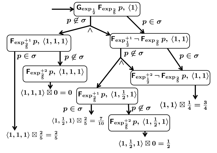
Example 4.1 (optimality not achievable).

Take a formula $\varphi=\mathop{\mathsf{G}\raisebox{-0.86108pt}[0.0pt][0.0pt]{$\scriptstyle\eta$}}\nolimits\mathsf{F}p$ and the Kripke structure $\mathcal{K}$ shown in the above. This example illustrates that the existence of an optimal path is not guaranteed in general: indeed, whereas $\sup_{\xi^{\prime}\in\mathop{\mathrm{path}}\nolimits(\mathcal{K})}\llbracket\xi^{\prime},\varphi\rrbracket=1$ in this example, there is no path $\xi$ that achieves $\llbracket\xi,\varphi\rrbracket=1$.

More specifically: we first note that, in each path $\xi$ of the Kripke structure, $p$ is true at most once. The later the state $s_{1}$ occurs in a path $\xi$, the bigger the truth value $\llbracket\xi,\varphi\rrbracket$ is; moreover the value $\llbracket\xi,\varphi\rrbracket$ tends to $1$ (since $\eta$ tends to $0$). However there is no path $\xi$ that achieves exactly $\llbracket\xi,\varphi\rrbracket=1$: if $p$ is postponed indefinitely, no state in $\xi$ satisfies $p$, in which case $\mathsf{F}p$ is everywhere false and hence $\llbracket\xi,\varphi\rrbracket=0$.

We thus strive for near-optimality, allowing a prescribed margin $\varepsilon$.

Definition 4.2.

The near-optimal scheduling problem for $\textrm{LTL}^{\mathrm{disc}}[\mathcal{D},\mathcal{F}]$ is: given a Kripke structure $\mathcal{K}=(W,R,\lambda)$, an $\textrm{LTL}^{\mathrm{disc}}[\mathcal{D},\mathcal{F}]$ formula $\varphi$ and a positive real number $\varepsilon\in(0,1)$, to find a path $\xi_{0}\in\mathop{\mathrm{path}}\nolimits(\mathcal{K})$ such that $\llbracket\xi_{0},\varphi\rrbracket\geq\sup_{\xi\in\mathop{\mathrm{path}}\nolimits(\mathcal{K})}\llbracket\xi,\varphi\rrbracket-\varepsilon$.

Ultimately we will show that the problem in the above is decidable (Thm. 4.14), when all the propositional quality operators are monotone and continuous ($\mathcal{F}\subseteq\mathcal{F}_{\mathrm{mc}}$).

We first note that, in the special case for $\textrm{LTL}^{\mathrm{disc}}[\mathcal{D},\emptyset]$ (i.e. no propositional quality operators), there is a straightforward binary search algorithm that relies on the (threshold) model-checking algorithm in [3] (Thm. 2.9). Specifically, the binary search algorithm repeatedly conducts threshold model-checking for: the threshold $v=\frac{1}{2}$ in the first round; $v=\frac{1}{4}$ or $\frac{3}{4}$ in the second round, depending on the outcome of the first round; then for $v=\frac{1}{8},\dotsc,\frac{6}{8}$ or $\frac{7}{8}$, depending on the outcome of the second round; and so on. Given a margin $\varepsilon\in(0,1)$, this way, we need $-\log\varepsilon$ rounds. This binary search algorithm is rather effective (see §5).

However the binary search algorithm does not work in presence of the average operator $\oplus$, simply because the threshold model-checking problem is undecidable (Thm. 2.10). Our main contribution is a novel algorithm for near-optimal scheduling that works even in this case (and more generally for the logic $\textrm{LTL}^{\mathrm{disc}}[\mathcal{D},\mathcal{F}_{\mathrm{mc}}]$). Our algorithm first translates a formula $\varphi$ and a margin $\varepsilon\in(0,1)$ to an alternating $[0,1]$-acceptance automaton $\mathcal{A}_{\varphi,\varepsilon}$, which is further turned into a $[0,1]$-acceptance automaton (Prop. 3.4). The resulting automaton—after taking the product with $\mathcal{K}$—is amenable to optimal value search (Lem. 3.2), yielding a solution to the original problem.

In the rest of the section we describe our algorithm. We shall however first restrict to the logic $\textrm{LTL}^{\mathrm{disc}}[\mathcal{D},\emptyset]$ for the sake of presentation (although this basic fragment allows binary search). After describing the basic algorithm for $\textrm{LTL}^{\mathrm{disc}}[\mathcal{D},\emptyset]$ in §4.1, in §4.2 we explain how it can be modified to accommodate propositional quality operators.

4.1. Our Algorithm, When Restricted to $\textrm{LTL}^{\mathrm{disc}}[\mathcal{D},\emptyset]$

Our translation of $\varphi$ and $\varepsilon\in(0,1)$ to an automaton $\mathcal{A}_{\varphi,\varepsilon}$ is an extension of the standard translation from LTL formulas to alternating Büchi automata (e.g. in [22]), with:

• incorporation of quantities—accumulation of discount factors, more specifically—by means of what we call discount sequences; and

• cutting off those events which are far in the future—the idea of event horizon from [3].

The extension is not complicated on the conceptual level. Its details need care, however, especially in handling negations and alternation of greatest and least fixed points.

As preparation, we recall some definitions and notations from [3].

Definition 4.3 ($\eta^{+k}$, $\mathit{xcl}(\varphi)$ [3]).

Let $\eta:\mathbb{N}\rightarrow[0,1]$ be a discounting function. We define a discounting function $\eta^{+k}:\mathbb{N}\rightarrow[0,1]$ by $\eta^{+k}(i)=\eta(i+k)$ for each $k\in\mathbb{N}$.

For an $\textrm{LTL}^{\mathrm{disc}}[\mathcal{D},\mathcal{F}]$ formula $\varphi$, the extended closure $\mathit{xcl}(\varphi)$ of $\varphi$ [3] is defined by

$$\mathit{xcl}(\varphi)\;=\;\mathop{\mathrm{Sub}}\nolimits(\varphi)\cup\{\varphi_{1}\mathbin{\mathsf{U}}_{\eta^{+k}}\varphi_{2}\mid k\in\mathbb{N},\varphi_{1}\mathbin{\mathsf{U}}_{\eta}\varphi_{2}\in\mathop{\mathrm{Sub}}\nolimits(\varphi)\}\enspace,$$ (5)

where $\mathop{\mathrm{Sub}}\nolimits(\varphi)$ denotes the set of subformulas of $\varphi$.

4.1.1. Discounting Sequences

We go on to technical details. In the alternating $[0,1]$-acceptance automaton $\mathcal{A}_{\varphi,\varepsilon}$ that we shall construct, a state is a pair $(\psi,\vec{d})$ of a formula $\psi$ and a discount sequence $\vec{d}\in[0,1]^{+}$.

Definition 4.4 (discount sequence).

A discount sequence is a sequence $\vec{d}=d_{1}d_{2}\dotsc d_{n}\in[0,1]^{+}$ of real numbers with a nonzero length ($d_{i}\in[0,1]$ for each $i$).

The notion of discount sequence is a quantitative extension of that of priority in parity automata. Specifically, the length $n$ of a discount sequence $\vec{d}=d_{1}d_{2}\dotsc d_{n}$ corresponds to a priority—i.e. the alternation depth of greatest and least fixed points. Each real number $d_{i}$ in the sequence, in turn, stands for the accumulated discount factor in each level of fixed-point alternation. For example, the formula $\mathop{\mathsf{F}\raisebox{-0.86108pt}[0.0pt][0.0pt]{$\scriptstyle\mathrm{exp}_{\frac{1}{2}}$}}\nolimits\mathop{\mathsf{G}\raisebox{-0.86108pt}[0.0pt][0.0pt]{$\scriptstyle\mathrm{exp}_{\frac{2}{3}}$}}\nolimits\mathop{\mathsf{F}\raisebox{-0.86108pt}[0.0pt][0.0pt]{$\scriptstyle\mathrm{exp}_{\frac{3}{4}}$}}\nolimits p$ will induce a discount sequence $(\frac{1}{2})^{n_{1}},(\frac{2}{3})^{n_{2}},(\frac{3}{4})^{n_{3}}$ of length 3—where $n_{1},n_{2}$ and $n_{3}$ are the numbers of steps for which the three discounting temporal operators $\mathop{\mathsf{F}\raisebox{-0.86108pt}[0.0pt][0.0pt]{$\scriptstyle\eta_{1}$}}\nolimits$, $\mathop{\mathsf{G}\raisebox{-0.86108pt}[0.0pt][0.0pt]{$\scriptstyle\eta_{2}$}}\nolimits$ and $\mathop{\mathsf{F}\raisebox{-0.86108pt}[0.0pt][0.0pt]{$\scriptstyle\eta_{3}$}}\nolimits$ “have waited,” respectively.

We use three operators $\odot,\mathbin{:},\boxtimes$ that act on discount sequences; the intuitions are as follows. The first two are for accumulating discount factors: we use $\odot$ in case there is no alternation of greatest and least fixed points; and we use $\mathbin{:}$ in case there is. Examples are:

$$\textstyle\begin{array}[]{lcl}\bigl{(}\,(\frac{1}{2})^{2},(\frac{2}{3})^{3},\frac{3}{4}\,\bigr{)}\;\odot\;\color[rgb]{0,0,1}\frac{4}{5}\color[rgb]{0,0,0}&=&\bigl{(}\,(\frac{1}{2})^{2},(\frac{2}{3})^{3},\frac{3}{4}\cdot\color[rgb]{0,0,1}\frac{4}{5}\color[rgb]{0,0,0}\,\bigr{)}\;=\;\bigl{(}\,(\frac{1}{2})^{2},(\frac{2}{3})^{3},\frac{3}{5}\,\bigr{)}\quad\text{and}\\ \bigl{(}\,(\frac{1}{2})^{2},(\frac{2}{3})^{3},\frac{3}{4}\,\bigr{)}\;\mathbin{:}\;\color[rgb]{0,0,1}\frac{4}{5}\color[rgb]{0,0,0}&=&\bigl{(}\,(\frac{1}{2})^{2},(\frac{2}{3})^{3},\frac{3}{4},\,\color[rgb]{0,0,1}\frac{4}{5}\color[rgb]{0,0,0}\,\bigr{)}\enspace.\end{array}$$

Note that in the former the length is preserved, while in the latter the sequence gets longer by one.

Definition 4.5 ($\vec{d}\odot d^{\prime}$, $\vec{d}\mathbin{:}d^{\prime}$).

The operator $\odot$ takes a discount sequence $\vec{d}$ and a discount factor $d^{\prime}\in[0,1]$ as arguments, and multiplies the last element of $\vec{d}$ by $d^{\prime}$. That is,

$$(d_{1}d_{2}\dotsc d_{n})\odot d^{\prime}\;=\;d_{1}d_{2}\dotsc d_{n-1}(d_{n}\cdot d^{\prime})\quad\in[0,1]^{+}\enspace.$$

The operator $\mathbin{:}$ is simply the concatenation operator: given $\vec{d}=d_{1}d_{2}\dotsc d_{n}$ and $d^{\prime}\in[0,1]$, the sequence $\vec{d}\mathbin{:}d^{\prime}$ is $d_{1}d_{2}\dotsc d_{n}d^{\prime}$ of length $n+1$.

We use the operator $\boxtimes$ in $\vec{d}\boxtimes v$ to let a discount sequence $\vec{d}$ act on a truth value $v\in[0,1]$.

Definition 4.6 ($\vec{d}\boxtimes v$).

The operator $\boxtimes$ takes $\vec{d}\in[0,1]^{+}$ and $v\in[0,1]$ as arguments. The value $\vec{d}\boxtimes v\in[0,1]$ is defined inductively by:

$$d\boxtimes v\;=\;dv\enspace,\qquad\vec{d}d^{\prime}\boxtimes v\;=\;\vec{d}\boxtimes(1-d^{\prime}v)\enspace.\quad\text{Explicitly:}$$ (6)

$$\footnotesize\begin{array}[]{l}(d_{1}d_{2}\dotsc d_{n})\boxtimes v\;=\;d_{1}\,-d_{1}d_{2}\,+d_{1}d_{2}d_{3}\,-\cdots\,+(-1)^{n}d_{1}d_{2}\dotsc d_{n-1}\,+(-1)^{n+1}d_{1}d_{2}\dotsc d_{n}v\,.\end{array}$$ (8)

The intuition behind the action $\vec{d}\boxtimes v$ is most visible in (6), where $dv$ and $d^{\prime}v$ denote multiplication of real numbers. Given a discount sequence $\vec{d}d^{\prime}$: 1) we apply the final discount factor $d^{\prime}$ to the truth value $v$, obtaining $d^{\prime}v$; 2) the alternation between greatest and least fixed points is taken into account, by taking the negation $1-d^{\prime}v$ (cf. Def. 2.5); and 3) we apply the remaining sequence $\vec{d}$ inductively and obtain $\vec{d}\boxtimes(1-d^{\prime}v)$. An example is $\textstyle\bigl{(}\frac{3}{4},\,\frac{1}{3},\,\frac{2}{5}\bigr{)}\boxtimes 1=\bigl{(}\frac{3}{4},\,\frac{1}{3}\bigr{)}\boxtimes\bigl{(}1-\frac{2}{5}\cdot 1\bigr{)}=\bigl{(}\frac{3}{4},\,\frac{1}{3}\bigr{)}\boxtimes\frac{3}{5}=\bigl{(}\frac{3}{4}\bigr{)}\boxtimes\bigl{(}1-\frac{1}{3}\cdot\frac{3}{5}\bigr{)}=\bigl{(}\frac{3}{4}\bigr{)}\boxtimes\frac{4}{5}=\frac{3}{5}$.

The following relationship between $\odot$ and $\boxtimes$ is easily seen to hold:

$$(\vec{d}\odot d^{\prime})\boxtimes v\;=\;\vec{d}\boxtimes(d^{\prime}\cdot v)\enspace.$$ (9)

The three operators $\odot,\mathbin{:},\boxtimes$ defined in the above will be used shortly, in the construction of the automaton $\mathcal{A}_{\varphi,\varepsilon}$. Their roles are briefly discussed after Def. 4.7.

4.1.2. Construction of $\mathcal{A}_{\varphi,\varepsilon}$

We describe the construction of $\mathcal{A}_{\varphi,\varepsilon}$, for a formula $\varphi$ of $\textrm{LTL}^{\mathrm{disc}}[\mathcal{D},\emptyset]$ and a margin $\varepsilon$. We subsequently discuss ideas behind it, comparing the definition with other known constructions.

We first define $\mathcal{A}^{\mathrm{p}}_{\varphi,\varepsilon}$ that is infinite-state, and obtain $\mathcal{A}_{\varphi,\varepsilon}$ as the reachable part. The latter will be shown to be finite-state (Lem. 4.8).

Definition 4.7 (the automata $\mathcal{A}^{\mathrm{p}}_{\varphi,\varepsilon},\mathcal{A}_{\varphi,\varepsilon}$).

Let $\varphi$ be an $\textrm{LTL}^{\mathrm{disc}}[\mathcal{D},\emptyset]$ formula and $\varepsilon\in(0,1)$. We define an alternating $[0,1]$-acceptance automaton $\mathcal{A}^{\mathrm{p}}_{\varphi,\varepsilon}=(\mathcal{P}(\mathit{AP}),Q,I,\delta,F)$ as follows. Its state space $Q$ is $\mathit{xcl}(\varphi)\times[0,1]^{+}$; hence a state is a pair $(\psi,\vec{d})$ of a formula and a discount sequence. The transition function $\delta\colon Q\times\mathcal{P}(\mathit{AP})\to\mathcal{B}^{+}(Q\cup[0,1])$ is defined as in Table 1, where we let $\vec{d}=d_{1}d_{2}\ldots d_{n}\in[0,1]^{+}$ and $\sigma\in\mathcal{P}(\mathit{AP})$.

$$\delta\bigl{(}(\mathtt{True},\vec{d}),\sigma\bigr{)} =\vec{d}\boxtimes 1$$

$$\delta\bigl{(}(p,\vec{d}),\sigma\bigr{)} =\begin{cases}\vec{d}\boxtimes 1&\mbox{if }p\in\sigma,\\ \vec{d}\boxtimes 0&\mbox{otherwise.}\end{cases}$$

$$\delta\bigl{(}(\lnot\psi,\vec{d}),\sigma\bigr{)} =\delta\bigl{(}(\psi,\vec{d}\mathbin{:}1),\sigma\bigr{)}$$ (10)

$$\delta\bigl{(}(\psi_{1}\land\psi_{2},\vec{d}),\sigma\bigr{)} =\begin{cases}{\delta\bigl{(}(\psi_{1},\vec{d}),\sigma\bigr{)}}\land{\delta\bigl{(}(\psi_{2},\vec{d}),\sigma\bigr{)}}&\mbox{if $|\vec{d}|$ is odd},\\ {\delta\bigl{(}(\psi_{1},\vec{d}),\sigma\bigr{)}}\lor{\delta\bigl{(}(\psi_{2},\vec{d}),\sigma\bigr{)}}&\mbox{otherwise.}\end{cases}$$

$$\delta\bigl{(}(\mathsf{X}\psi,\vec{d}),\sigma\bigr{)} =(\psi,\vec{d})$$

$$\delta\bigl{(}(\psi_{1}\mathbin{\mathsf{U}}\psi_{2},\vec{d}),\sigma\bigr{)} =\begin{cases}{\delta\bigl{(}(\psi_{2},\vec{d}),\sigma\bigr{)}}\lor\Bigl{(}\,{\delta\bigl{(}(\psi_{1},\vec{d}),\sigma\bigr{)}}\land{(\psi_{1}\mathbin{\mathsf{U}}\psi_{2},\vec{d})}\,\Bigr{)}&\mbox{if $|\vec{d}|$ is odd},\\ {\delta\bigl{(}(\psi_{2},\vec{d}),\sigma\bigr{)}}\land\Bigl{(}\,{\delta\bigl{(}(\psi_{1},\vec{d}),\sigma\bigr{)}}\lor{(\psi_{1}\mathbin{\mathsf{U}}\psi_{2},\vec{d})}\,\Bigr{)}&\mbox{otherwise.}\end{cases}$$

For $\delta\bigl{(}(\psi_{1}\mathbin{\mathsf{U}}_{\eta}\psi_{2},\vec{d}),\sigma\bigr{)}$ we make cases. Let $\vec{d}=d_{1}\dotsc d_{n}$. If $\eta(0)\cdot\prod_{i=1}^{n}d_{i}\leq\varepsilon$:

$$\small\delta\bigl{(}(\psi_{1}\mathbin{\mathsf{U}}_{\eta}\psi_{2},\vec{d}),\sigma\bigr{)}=\begin{cases}\vec{d}\boxtimes 0&\mbox{if $|\vec{d}|$ is odd},\\ \vec{d}\boxtimes\eta(0)&\mbox{otherwise;}\end{cases}$$ (11)

otherwise, i.e. if $\eta(0)\cdot\prod_{i=1}^{n}d_{i}>\varepsilon$:

$$\delta\bigl{(}(\psi_{1}\mathbin{\mathsf{U}}_{\eta}\psi_{2},\vec{d}),\sigma\bigr{)}=\begin{cases}{\delta\bigl{(}(\psi_{2},\vec{d}\odot\eta(0)),\sigma\bigr{)}}\lor\Bigl{(}{\delta\bigl{(}(\psi_{1},\vec{d}\odot\eta(0)),\sigma\bigr{)}}\land{(\psi_{1}\mathbin{\mathsf{U}}_{\eta^{+1}}\psi_{2},\vec{d})}\Bigr{)}&\mbox{if $|\vec{d}|$ is odd},\\ {\delta\bigl{(}(\psi_{2},\vec{d}\odot\eta(0)),\sigma\bigr{)}}\land\Bigl{(}{\delta\bigl{(}(\psi_{1},\vec{d}\odot\eta(0)),\sigma\bigr{)}}\lor{(\psi_{1}\mathbin{\mathsf{U}}_{\eta^{+1}}\psi_{2},\vec{d})}\Bigr{)}&\mbox{otherwise.}\end{cases}$$ (12)

Table 1. Transition function $\delta$ of $\mathcal{A}^{\mathrm{p}}_{\varphi,\varepsilon}$

The set $I$ of the initial states of $\mathcal{A}^{\mathrm{p}}_{\varphi,\varepsilon}$ is $\{(\varphi,1)\}$. The acceptance function $F$ is

$$\small F(\psi,\vec{d})=\begin{cases}1&\mbox{if }{\psi=\psi_{1}\mathbin{\mathsf{U}}\psi_{2}}\mbox{ and $|\vec{d}|$ is even}\\ 0&\mbox{otherwise.}\end{cases}$$ (13)

The alternating $[0,1]$-acceptance automaton $\mathcal{A}_{\varphi,\varepsilon}$ is defined to be the restriction of $\mathcal{A}^{\mathrm{p}}_{\varphi,\varepsilon}$ to the states that are reachable from the initial state $(\varphi,1)$.

Examples of $\mathcal{A}_{\varphi,\varepsilon}$ are in Fig. 2–2, where $(\varphi,\varepsilon)=(\mathop{\mathsf{G}\raisebox{-0.86108pt}[0.0pt][0.0pt]{$\scriptstyle\mathrm{exp}_{\frac{1}{2}}$}}\nolimits\mathop{\mathsf{F}\raisebox{-0.86108pt}[0.0pt][0.0pt]{$\scriptstyle\mathrm{exp}_{\frac{2}{5}}$}}\nolimits p,\frac{1}{3})$ and $(\mathop{\mathsf{F}\raisebox{-0.86108pt}[0.0pt][0.0pt]{$\scriptstyle\mathrm{exp}_{\frac{1}{2}}$}}\nolimits\mathsf{G}p,\frac{1}{3})$. There a discount sequence $d_{1}\dotsc d_{n}$ is denoted by $\langle d_{1},\dotsc,d_{n}\rangle$ for readability.

Figure 1. The automaton $\mathcal{A}_{\varphi,\varepsilon}$ for
$\varphi=\mathop{\mathsf{G}\raisebox{-0.86108pt}[0.0pt][0.0pt]{$\scriptstyle\mathrm{exp}_{\frac{1}{2}}$}}\nolimits\mathop{\mathsf{F}\raisebox{-0.86108pt}[0.0pt][0.0pt]{$\scriptstyle\mathrm{exp}_{\frac{2}{5}}$}}\nolimits p$ and $\varepsilon=\frac{1}{3}$

Figure 2. The automaton $\mathcal{A}_{\varphi,\varepsilon}$ for
$\varphi=\mathop{\mathsf{F}\raisebox{-0.86108pt}[0.0pt][0.0pt]{$\scriptstyle\mathrm{exp}_{\frac{1}{2}}$}}\nolimits\mathsf{G}p$ and $\varepsilon=\frac{1}{3}$. The double-lined nodes have the acceptance value $1$.

Some remarks on Def. 4.7 are in order.

In Absence of Discounting (Sanity Check) If the formula $\varphi$ contains no discounting operator $\mathbin{\mathsf{U}}_{\eta}$, then the construction essentially coincides the usual one in [22] that translates a (usual) LTL formula to an alternating Büchi automaton. To see it, recall that the length $|\vec{d}|$ of a discount sequence plays the role of a priority in parity automata (§4.1.1). Therefore in the first case of (13), $|\vec{d}|$ being even means that we are in fact dealing with a greatest fixed point. This makes the state accepting (in the Büchi sense), much like in [22].

$\mathcal{A}_{\varphi,\varepsilon}$ is Quantitative  The acceptance values of the states of $\mathcal{A}_{\varphi,\varepsilon}$ are Boolean (see (13)). Nevertheless the automaton is quantitative, in that non-Boolean values from $[0,1]$ appear as atomic propositions in the range $\mathcal{B}^{+}(Q\cup[0,1])$ of the transition $\delta$ (they occur at the leaves in Fig. 2–2). Once we transform $\mathcal{A}_{\varphi,\varepsilon}$ to a non-alternating automaton (Prop. 3.4), these non-Boolean propositional values give rise to non-Boolean acceptance values.

Event Horizon  A fundamental idea from [3] is the following. A discounting operator, in presence of a threshold (in [3]) or a nonzero margin (here), allows an exact representation by a (finitary) formula without a fixed point operator. The latter means, for example:

$$\textstyle\llbracket\pi,\mathop{\mathsf{F}\raisebox{-0.86108pt}[0.0pt][0.0pt]{$\scriptstyle\mathrm{exp}_{\frac{1}{2}}$}}\nolimits\varphi\rrbracket\geq\frac{1}{4} \quad\Longleftrightarrow\quad\pi\models\varphi\lor\mathsf{X}\varphi\lor\mathsf{X}\mathsf{X}\varphi\enspace,\quad\text{and}$$ (14)

$$\textstyle\llbracket\pi,\mathop{\mathsf{G}\raisebox{-0.86108pt}[0.0pt][0.0pt]{$\scriptstyle\mathrm{exp}_{\frac{1}{2}}$}}\nolimits\varphi\rrbracket\geq\frac{3}{4} \quad\Longleftrightarrow\quad\pi\models\varphi\land\mathsf{X}\varphi\land\mathsf{X}\mathsf{X}\varphi\enspace,$$ (15)

and so on. Note that in (14), whatever happens after two time units has contributions less than $(\frac{1}{2})^{2}=\frac{1}{4}$ and therefore never enough to make up the threshold. The example (15) is similar, with events in the future having only negligible negative contributions. In other words: fixed point operators with discounting have an event horizon—in the above examples (14–15) it lies between $t=2$ and $3$—nothing beyond which matters.

This idea of event horizon is used in the distinction between (11) and (12). The value $\eta(0)\cdot\prod_{i=1}^{n}d_{i}$ is, as we shall see, the greatest contribution to a truth value that the events henceforth potentially have. In case it is smaller than the margin $\varepsilon$ we can safely ignore the positive contribution henceforth and take the smallest possible truth value $0$—much like the disjunct $\mathsf{X}^{3}\varphi\lor\mathsf{X}^{4}\varphi\lor\cdots$ is truncated in (14). This is what is done in the first case in (11). The second case in (11) is about a greatest fixed point and we truncate the negative contributions of the events beyond the event horizon—this is much like the obligation $\mathsf{X}^{3}\varphi\land\mathsf{X}^{4}\varphi\land\cdots$ is lifted in (15). In this case we use the greatest truth value possible, namely $\eta(0)$. This is what is done in (11).

Use of Discount Sequences  Discount sequences $\vec{d}$ are used for two purposes. Firstly, as we already described, its length $|\vec{d}|$ indicates the alternation between positive and negative views on a formula—observe that a discount sequence gets longer in (10). Consequently many clauses in the definition of $\delta$ distinguish cases according to the parity of $|\vec{d}|$. Secondly it records all the discount factors that have been encountered. See (12), where the last element of $\vec{d}$ is multiplied by the newly encountered factor $\eta(0)$ and updated to $\vec{d}\odot\eta(0)$. Such accumulation $\vec{d}$ of discount factors acts on a truth value via the $\boxtimes$ operator, like in (11) and in the definition of $\delta\bigl{(}(\mathtt{True},\vec{d}),\sigma\bigr{)}$.

Lemma 4.8.

The automaton $\mathcal{A}_{\varphi,\varepsilon}$ has only finitely many states. ∎

The following “correctness lemma” claims that $\mathcal{A}_{\varphi,\varepsilon}$ conducts the expected task.

Lemma 4.9.

Let $\varphi$ be an $\textrm{LTL}^{\mathrm{disc}}[\mathcal{D},\emptyset]$ formula and $\varepsilon\in(0,1)$ be a positive real number. For each computation $\pi\in(\mathcal{P}(\mathit{AP}))^{\omega}$, we have $\llbracket\pi,\varphi\rrbracket-\varepsilon\;\leq\;\mathcal{L}(\mathcal{A}_{\varphi,\varepsilon})(\pi)\;\leq\;\llbracket\pi,\varphi\rrbracket$∎

4.1.3. The Algorithm

After the construction of $\mathcal{A}_{\varphi,\varepsilon}$, the algorithm proceeds in the following manner. We first translate $\mathcal{A}_{\varphi,\varepsilon}$ to a (non-alternating) $[0,1]$-acceptance automaton (relying on Prop. 3.4).

Corollary 4.10.

Let $\varphi$ be an $\textrm{LTL}^{\mathrm{disc}}[\mathcal{D},\emptyset]$ formula and $\varepsilon\in(0,1)$ be a positive real number. There exists a (non-alternating) $[0,1]$-acceptance automaton $\mathcal{A}^{\mathrm{na}}_{\varphi,\varepsilon}$ such that $\llbracket\pi,\varphi\rrbracket-\varepsilon\leq\mathcal{L}(\mathcal{A}^{\mathrm{na}}_{\varphi,\varepsilon})(\pi)\leq\llbracket\pi,\varphi\rrbracket$ for each computation $\pi\in(\mathcal{P}(\mathit{AP}))^{\omega}$. ∎

Towards the solution of the near-optimal scheduling problem (Def. 4.2), we construct the product of $\mathcal{A}^{\mathrm{na}}_{\varphi,\varepsilon}$ in Cor. 4.10 and the given Kripke structure $\mathcal{K}$. Since transitions of $[0,1]$-acceptance automata are nondeterministic, this product can be defined just as usual.

Definition 4.11.

Let $\mathcal{A}=(\mathcal{P}(\mathit{AP}),Q,I,\delta,F)$ be a $[0,1]$-acceptance automaton and $\mathcal{K}=(W,R,\lambda)$ be a Kripke structure. Their product $\mathcal{A}\times\mathcal{K}$ is a $[0,1]$-acceptance automaton $(1,Q^{\prime},I^{\prime},\delta^{\prime},F^{\prime})$—over a singleton alphabet $1=\{\bullet\}$—defined by: $Q^{\prime}=Q$; $I^{\prime}=I\times W$; $\delta^{\prime}\bigl{(}\,(q,s),\,\bullet\,\bigr{)}=\bigl{\{}\,(q^{\prime},s^{\prime})\;\bigl{|}\bigr{.}\;q^{\prime}\in\delta(q,\lambda(s)),(s,s^{\prime})\in R\,\bigr{\}}$; and $F^{\prime}(q,s)=F(q)$.

Lemma 4.12.

Let $(q_{0},s_{0})\,\bullet\,(q_{1},s_{1})\,\bullet\,\dotsc$ be an optimal run of the automaton $\mathcal{A}\times\mathcal{K}$ (that necessarily exists by Lem. 3.2). The path $s_{0}s_{1}\dotsc\in\mathop{\mathrm{path}}\nolimits(\mathcal{K})$ realizes the optimal value of $\mathcal{A}$, that is, $\mathcal{L}(\mathcal{A})\bigl{(}\lambda(s_{0})\lambda(s_{1})\dotsc\bigr{)}=\max_{\xi\in\mathop{\mathrm{path}}\nolimits(\mathcal{K})}\mathcal{L}(\mathcal{A})\bigl{(}\lambda(\xi)\bigr{)}$. ∎

Theorem 4.13 (optimal scheduling for $\textrm{LTL}^{\mathrm{disc}}[\mathcal{D},\emptyset]$).

Assume the setting of Def. 4.2, and that $\mathcal{F}=\emptyset$ (i.e. the formula $\varphi$ contains no propositional quality operators). Let $(q_{0},s_{0})\,\bullet\,(q_{1},s_{1})\,\bullet\,\dotsc$ be an optimal run (computed by Lem. 3.2) for the $[0,1]$-acceptance automaton $\mathcal{A}^{\mathrm{na}}_{\varphi,\varepsilon}\times\mathcal{K}$ constructed as in Def. 4.7, Cor. 4.10 and Def. 4.11. Then the path $s_{0}s_{1}\dotsc\in\mathop{\mathrm{path}}\nolimits(\mathcal{K})$ is a solution to the near-optimal scheduling problem (Def. 4.2).

Moreover, the solution $s_{0}s_{1}\dotsc$ can be chosen to be ultimately periodic. ∎

4.2. Our General Algorithm for $\textrm{LTL}^{\mathrm{disc}}[\mathcal{D},\mathcal{F}_{\mathrm{mc}}]$

Our general algorithm works in the setting of $\textrm{LTL}^{\mathrm{disc}}[\mathcal{D},\mathcal{F}_{\mathrm{mc}}]$—i.e. in the presence of monotone and continuous propositional quality operators like $\oplus$—where threshold model checking is potentially undecidable [3] and therefore the binary-search algorithm (described after Def. 4.2) may not work.

The general algorithm is a (rather straightforward) adaptation of the one we described for $\textrm{LTL}^{\mathrm{disc}}[\mathcal{D},\emptyset]$ (§4.1). Here we construct the alternating $[0,1]$-acceptance automaton $\mathcal{A}_{\varphi,\varepsilon}$ inductively on the construction on the formula $\varphi$:

• When the outermost connective is other than a propositional quality operator, the construction is much like in Def. 4.7.

• When the outermost connective is a propositional quality operator, we rely on Prop. 3.5.

The rest of the algorithm (i.e. the part described in §4.1.3) remains unchanged. An extensive description of the details of the construction is deferred to Appendix A.

Theorem 4.14 (main theorem, optimal scheduling for $\textrm{LTL}^{\mathrm{disc}}[\mathcal{D},\mathcal{F}_{\mathrm{mc}}]$).

In the setting of Def. 4.2, assume that $\mathcal{F}\subseteq\mathcal{F}_{\mathrm{mc}}$ (i.e. all the propositional quality operators in $\varphi$ are monotone and continuous). Then the near-optimal scheduling problem is decidable. ∎

4.3. Complexity

The two parameters $\mathcal{D}$ and $\mathcal{F}$ in $\textrm{LTL}^{\mathrm{disc}}[\mathcal{D},\mathcal{F}]$—i.e. discounting functions (Def. 2.1) and propositional quality operators (Def. 2.2)—are both relevant to the complexity of our algorithm. Formulating a complexity result is hard when these parameters are left open. We therefore restrict to:

• exponential discounting functions (Def. 2.1), i.e. $\mathcal{D}=\mathcal{D}_{\mathrm{exp}}=\{\mathrm{exp}_{\lambda}\mid\lambda\in(0,1)\cap\mathbb{Q}\}$, as is done in [3]; and

• the average operator $\oplus$, i.e. $\mathcal{F}=\{\oplus\}$.

We use the definition $|\langle\varphi\rangle|$ of the size of a formula $\varphi$, which is from [3]: it reflects the description length of $\lambda\in\mathbb{Q}$ that appears in discounting functions, as well as the length of $\varphi$ as an expression.

Proposition 4.15 (size of $\mathcal{A}_{\varphi,\varepsilon}$).

Let $\varphi$ be an $\textrm{LTL}^{\mathrm{disc}}[\mathcal{D}_{\mathrm{exp}},\{\oplus\}]$ formula and $\varepsilon\in(0,1)\cap\mathbb{Q}$ be a positive rational number. The size of the state space of the alternating $[0,1]$-acceptance automaton $\mathcal{A}_{\varphi,\varepsilon}$ is singly exponential in $|\langle\varphi\rangle|$ and in the length of the description of $\varepsilon$. ∎

Theorem 4.16 (complexity for $\textrm{LTL}^{\mathrm{disc}}[\mathcal{D}_{\mathrm{exp}},\{\oplus\}]$).

The near-optimal scheduling problem for $\textrm{LTL}^{\mathrm{disc}}[\mathcal{D}_{\mathrm{exp}},\{\oplus\}]$ is: in EXPSPACE in $|\langle\varphi\rangle|$ and in the description length of $\varepsilon$; and in NLOGSPACE in the size of $\mathcal{K}$. ∎

In case of absence of propositional quality operators (i.e. $\textrm{LTL}^{\mathrm{disc}}[\mathcal{D}_{\mathrm{exp}},\emptyset]$), we can further optimize the complexity by using a heuristic and avoiding the exponential blowup from $\mathcal{A}_{\varphi,\varepsilon}$ to $\mathcal{A}^{\mathrm{na}}_{\varphi,\varepsilon}$. This yields the following complexity result, which is also achievable by the binary-search algorithm.

Theorem 4.17 (complexity for $\textrm{LTL}^{\mathrm{disc}}[\mathcal{D}_{\mathrm{exp}},\emptyset]$).

The near-optimal scheduling problem for $\textrm{LTL}^{\mathrm{disc}}[\mathcal{D}_{\mathrm{exp}},\emptyset]$ is: in PSPACE in $|\langle\varphi\rangle|$ and in the description length of $\varepsilon$; and in NLOGSPACE in the size of $\mathcal{K}$. ∎

5. Experiments

We implemented our algorithm in §4 that solves the near-optimal scheduling for $\textrm{LTL}^{\mathrm{disc}}[\mathcal{D}_{\mathrm{exp}},\{\oplus\}]$. The implementation is in OCaml. The following experiments were on a MacBook Pro laptop with a Core i5 processor (2.7 GHz) and 16 GB RAM.

	$\varepsilon=\frac{1}{10}$		$\varepsilon=\frac{1}{50}$		$\varepsilon=\frac{1}{100}$
formula $\varphi$ \  #(states)	$\mathcal{A}_{\varphi,\varepsilon}$	$\mathcal{A}^{\mathrm{na}}_{\varphi,\varepsilon}$	$\mathcal{A}_{\varphi,\varepsilon}$	$\mathcal{A}^{\mathrm{na}}_{\varphi,\varepsilon}$	$\mathcal{A}_{\varphi,\varepsilon}$	$\mathcal{A}^{\mathrm{na}}_{\varphi,\varepsilon}$
${\mathsf{F}_{\mathrm{exp}_{\frac{1}{2}}}p_{1}}$	5	10	7	14	8	16
${\mathsf{F}_{\mathrm{exp}_{\frac{99}{100}}}p_{1}}$	231	462	391	782	460	920
${\mathsf{F}_{\mathrm{exp}_{\frac{1}{2}}}\mathsf{G}_{\mathrm{exp}_{\frac{1}{2}}}p_{1}}$	15	36	28	85	36	121
${\mathsf{F}_{\mathrm{exp}_{\frac{1}{2}}}p_{1}}\oplus{\mathsf{F}_{\mathrm{exp}_{\frac{1}{2}}}p_{2}}$	33	128	61	1859	78	7421
${\mathsf{F}_{\mathrm{exp}_{\frac{1}{2}}}p_{1}}\oplus{\mathsf{G}_{\mathrm{exp}_{\frac{1}{2}}}p_{2}}$	29	272	55	6659	71	32703
${\mathsf{F}_{\mathrm{exp}_{\frac{3}{5}}}p_{1}}\oplus{\mathsf{F}_{\mathrm{exp}_{\frac{3}{5}}}p_{2}}$	46	477	97	29655	141	timeout (2 min.)
${\mathsf{F}(\mathsf{G}p_{1}\oplus\mathsf{F}_{\mathrm{exp}_{\frac{1}{2}}}p_{2})}$	14	19	20	27	23	31

Table 2. Size of the alternating $[0,1]$-acceptance automaton $\mathcal{A}_{\varphi,\varepsilon}$, and $[0,1]$-acceptance automaton $\mathcal{A}_{\varphi,\varepsilon}$

margin $\varepsilon$	#(states of $\mathcal{K}$)	max. outgoing degree of $\mathcal{K}$	time (sec)	space (MB)
$\frac{1}{10}$	100	3	0.085508	5.861
		10	0.114427	9.368
	200	3	0.186989	10.586
		10	0.249392	18.216
$\frac{1}{50}$	100	3	5.928842	199.782
		10	8.108335	405.884
	200	3	10.750703	405.313
		10	18.250345	851.255

Table 3. Time and space consumption of our algorithm for near-optimal scheduling, for the formula ${\mathop{\mathsf{G}\raisebox{-0.60275pt}[0.0pt][0.0pt]{$\scriptstyle\mathrm{exp}_{\frac{1}{2}}$}}\nolimits p_{1}}\oplus{\mathop{\mathsf{G}\raisebox{-0.60275pt}[0.0pt][0.0pt]{$\scriptstyle\mathrm{exp}_{\frac{1}{2}}$}}\nolimits p_{2}}$ and a randomly generated Kripke structure $\mathcal{K}$. For each choice of the number of states ($100$ or $200$) and of the maximum outgoing degree ($3$ or $10$), we randomly generated $100$ instances of $\mathcal{K}$ and the above shows the average

	$\mathsf{G}_{\mathrm{exp}_{\frac{1}{2}}}\mathsf{F}p$		$\mathsf{F}_{\mathrm{exp}_{\frac{1}{2}}}\mathsf{G}p$
	time (sec)	space (MB)	time (sec)	space (MB)
our algorithm (§4.1)	18.918600	897.111	0.019800	4.629
binary search	0.047200	5.140390	0.069500	5.567

Table 4. (Comparison with binary search, in absence of $\oplus$) Time and space consumption for near-optimal scheduling, for the margin $\varepsilon=\frac{1}{100}$ and a randomly generated Kripke structure $\mathcal{K}$ ($500$ states, max. outgoing degree $10$, average over $100$ instances)

In Table 4, for each choice of $\varphi$ and $\varepsilon$, we show the size of the alternating automaton $\mathcal{A}_{\varphi,\varepsilon}$, and the non-alternating $\mathcal{A}^{\mathrm{na}}_{\varphi,\varepsilon}$ that results from $\mathcal{A}_{\varphi,\varepsilon}$. The first three rows have no $\oplus$, in which case the implementation scales well for bigger bases (i.e. discount functions that decrease more slowly). We observe that presence of $\oplus$ incurs substantial computational costs: the small increase of bases from $\frac{1}{2}$ (the fourth row) to $\frac{3}{5}$ (the sixth row) makes $\mathcal{A}_{\varphi,\varepsilon}$ much bigger, resulting in one timeout. This is as expected, however: $\oplus$ makes other problems harder too, such as model checking (undecidable).

In Table 4 we fix a formula $\varphi={\mathop{\mathsf{G}\raisebox{-0.86108pt}[0.0pt][0.0pt]{$\scriptstyle\mathrm{exp}_{\frac{1}{2}}$}}\nolimits p_{1}}\oplus{\mathop{\mathsf{G}\raisebox{-0.86108pt}[0.0pt][0.0pt]{$\scriptstyle\mathrm{exp}_{\frac{1}{2}}$}}\nolimits p_{2}}$ and measure time and space consumption, for various choices of a margin $\varepsilon$ and a Kripke structure $\mathcal{K}$. Kripke structures $\mathcal{K}$ were randomly generated: we first set the number of states (100 or 200) and the maximum outgoing degree of $\mathcal{K}$ (3 or 10); for each state we fixed its outgoing degree, from the uniform distribution from $1$ to the maximum (that we had already fixed); and then, for each outgoing edge, its target state is chosen from the uniform distribution over the set of states. We observe that time and space consumption grows significantly as the problem becomes more difficult. However, for problem instances of a considerable size we still see manageable costs: a margin $\varepsilon=\frac{1}{50}$ (2%) is fairly small, and a Kripke structure $\mathcal{K}$ with $200$ states is likely to be capable of modeling many communication protocols.

In Table 4, for reference, we compare our algorithm in §4.1 with the binary-search algorithm that exploits the model-checking algorithm in [3] (we also implemented the latter). We emphasize again that the latter does not work in presence of $\oplus$. Our experience shows that the binary-search algorithm can in some cases be faster by a magnitude (e.g. for the first formula here), but not always (for the second formula our algorithm is a few times faster).

Those experimental results indicate that, although presence of the average operator $\oplus$ incurs significant computational cost (as expected), automata-based optimal scheduling for $\textrm{LTL}^{\mathrm{disc}}[\mathcal{D}_{\mathrm{exp}},\{\oplus\}]$ is potentially a viable approach. It is not that our algorithm scales up to huge problem instances, but systems of hundreds of states can be handled without difficulties. Identification of concrete real-world challenges, and enhancement of the tool’s efficiency to match up to them, is an important direction of future work.

6. Conclusions and Future Work

For the quantitative logic $\textrm{LTL}^{\mathrm{disc}}[\mathcal{D}_{\mathrm{exp}},\mathcal{F}]$ with future discounting [3], we formulated a natural problem of synthesizing near-optimal schedulers, and presented an algorithm. The latter relies on: the existing idea of event horizon exploited in [3] for the threshold model checking problem, as well as a supposedly widely-applicable technique of translation to $[0,1]$-acceptance automata and a lasso-style optimal value algorithm for them.

Here are several directions of future work.

Controller Synthesis for Open Systems We note that the current results are focused on closed systems. For open or reactive systems (like a server that responds to requests that come from the environment) we would wish to synthesize a controller—formally a strategy or a transducer—that achieves a near-optimal performance.

An envisaged workflow, following the one in [22], is as follows. We will use the same automaton $\mathcal{A}_{\varphi,\varepsilon}$ (Def. 4.7). It is then: 1) determinized, 2) transformed into a tree automaton that accepts the desired strategies, and 3) the optimal value of the tree automaton is checked, much like in Lem. 3.2. While the step 2) will be straightforward, the steps 1) and 3) (namely: determinization of $[0,1]$-acceptance automata, and the optimal value problem for “$[0,1]$-acceptance Rabin automata”) are yet to be investigated. Another possible workflow is by an adaptation of the Safraless algorithm [16].

Probabilistic Systems and $\textrm{LTL}^{\mathrm{disc}}[\mathcal{D}_{\mathrm{exp}},\mathcal{F}]$ Here and in [3] the system model is a Kripke structure that is nondeterministic. Adding probabilistic branching will gives us a set of new problems to be solved: for Markov chains the threshold model-checking problem can be formulated; for Markov decision processes, we have both the threshold model-checking problem and the near-optimal scheduling problem. Furthermore, another axis of variation is given by whether we consider the expected value or the worst-case value. In the latter case we would wish to exclude truth values that arise with probability $0$. All these variations have important applications in various areas.

Acknowledgments

Thanks are due to Shaull Almagor, Shuichi Hirahara, and the anonymous referees, for useful discussions and comments. The authors are supported by Grants-in-Aid No. 24680001, 15KT0012 and 15K11984, JSPS.

Appendix A Our General Algorithm for $\textrm{LTL}^{\mathrm{disc}}[\mathcal{D},\mathcal{F}_{\mathrm{mc}}]$, Further Details

In this section, we extend §4.2 and describe details of the construction of $\mathcal{A}_{\varphi,\varepsilon}$ for a formula $\varphi$ of $\textrm{LTL}^{\mathrm{disc}}[\mathcal{D},\mathcal{F}_{\mathrm{mc}}]$. We inductively construct an alternating $[0,1]$-acceptance automaton $\mathcal{A}_{\varphi,\varepsilon}^{\vec{d}}$—that is also parametrized by a discount sequence $\vec{d}$. Then the automaton $\mathcal{A}_{\varphi,\varepsilon}$ is defined by $\mathcal{A}_{\varphi,\varepsilon}^{\langle 1\rangle}$ (for the sequence $\langle 1\rangle$ of length one).

Lemma A.1.

Let $\varphi$ be an $\textrm{LTL}^{\mathrm{disc}}[\mathcal{D},\mathcal{F}_{\mathrm{mc}}]$ formula, $\varepsilon\in(0,1)$ be a positive real number, and $\vec{d}=d_{1}d_{2}\dotsc d_{n}$ be a discount sequence (Def. 4.4). There exists an alternating $[0,1]$-acceptance automaton $\mathcal{A}_{\varphi,\varepsilon}^{\vec{d}}$ such that, for each computation $\pi\in(\mathcal{P}(\mathit{AP}))^{\omega}$,

$$\bigl{(}\vec{d}\boxtimes\llbracket\pi,\varphi\rrbracket\bigr{)}-\varepsilon\;\leq\;\mathcal{L}(\mathcal{A}^{\vec{d}}_{\varphi,\varepsilon})(\pi)\;\leq\;\vec{d}\boxtimes\llbracket\pi,\varphi\rrbracket\enspace.$$ (16)

Proof.

The proof is inductive on the construction of $\varphi$. In this proof we assume without loss of generality that an alternating $[0,1]$-acceptance automaton has exactly one initial state, and consequently, the initial state of $\mathcal{A}_{\varphi,\varepsilon}^{\vec{d}}$ shall be denoted by $q_{\varphi,\varepsilon}^{\vec{d}}$. For the case where the outermost connective of $\varphi$ is other than a propositional quality operator, we only describe the construction of $\mathcal{A}_{\varphi,\varepsilon}^{\vec{d}}$. The correctness of this automaton can be proved in a similar way to the proof of Lem. 4.9: recall that Lem. 4.9 is also proved by induction on the construction of a formula.

Suppose that $\varphi=\mathtt{True}$. We define $\mathcal{A}_{\mathtt{True},\varepsilon}^{\vec{d}}=(\mathcal{P}(\mathit{AP}),\{q_{\mathtt{True},\varepsilon}^{\vec{d}}\},\{q_{\mathtt{True},\varepsilon}^{\vec{d}}\},\delta,F)$ where $\delta(q_{\mathtt{True},\varepsilon}^{\vec{d}},\sigma)=\vec{d}\boxtimes 1$ and $F(q_{\mathtt{True},\varepsilon}^{\vec{d}})=0$.

Suppose that $\varphi=p\in\mathit{AP}$. We define $\mathcal{A}_{p,\varepsilon}^{\vec{d}}=(\mathcal{P}(\mathit{AP}),\{q_{p,\varepsilon}^{\vec{d}}\},\{q_{p,\varepsilon}^{\vec{d}}\},\delta,F)$ where

$$\delta(q_{p,\varepsilon}^{\vec{d}},\sigma)=\begin{cases}\vec{d}\boxtimes 1&\mbox{if }p\in\sigma\\ \vec{d}\boxtimes 0&\mbox{otherwise}\end{cases}\quad\mbox{ and }\quad F(q_{p,\varepsilon}^{\vec{d}})=0\enspace.$$

Suppose that $\varphi=\varphi_{1}\land\varphi_{2}$ and that $|\vec{d}|$ is odd. By the induction hypothesis, for each of $i\in\{1,2\}$, there exists $\mathcal{A}_{\varphi_{i},\varepsilon}^{\vec{d}}=(\mathcal{P}(\mathit{AP}),Q_{i},\{q_{\varphi_{i},\varepsilon}^{\vec{d}}\},\delta_{i},F_{i})$ that satisfies the postulated condition. Then we define $\mathcal{A}_{\varphi,\varepsilon}^{\vec{d}}=(\mathcal{P}(\mathit{AP}),Q,\{q_{\varphi,\varepsilon}^{\vec{d}}\},\delta,F)$ as follows. Its state space $Q$ is $\{q_{\varphi,\varepsilon}^{\vec{d}}\}\cup Q_{1}\cup Q_{2}$. The transition function $\delta$ is

$$\delta(q,\sigma)=\begin{cases}\delta_{1}(q_{\varphi_{1},\varepsilon}^{\vec{d}},\sigma)\land\delta_{2}(q_{\varphi_{2},\varepsilon}^{\vec{d}},\sigma)&\mbox{if }q=q_{\varphi,\varepsilon}^{\vec{d}}\\ \delta_{i}(q,\sigma)&\mbox{if }q\in Q_{i}.\end{cases}$$

The acceptance function $F$ is

$$F(q)=\begin{cases}0&\mbox{if }q=q_{\varphi,\varepsilon}^{\vec{d}}\\ F_{i}(q)&\mbox{if }q\in Q_{i}.\end{cases}$$

Suppose that $\varphi=\varphi_{1}\land\varphi_{2}$ and that $|\vec{d}|$ is even. By the induction hypothesis, for each of $i\in\{1,2\}$, there exists $\mathcal{A}_{\varphi_{i},\varepsilon}^{\vec{d}}=(\mathcal{P}(\mathit{AP}),Q_{i},\{q_{\varphi_{i},\varepsilon}^{\vec{d}}\},\delta_{i},F_{i})$ that satisfies the postulated condition. Then we define $\mathcal{A}_{\varphi,\varepsilon}^{\vec{d}}=(\mathcal{P}(\mathit{AP}),Q,\{q_{\varphi,\varepsilon}^{\vec{d}}\},\delta,F)$ as follows. Its state space $Q$ is $\{q_{\varphi,\varepsilon}^{\vec{d}}\}\cup Q_{1}\cup Q_{2}$. The transition function $\delta$ is

$$\delta(q,\sigma)=\begin{cases}\delta_{1}(q_{\varphi_{1},\varepsilon}^{\vec{d}},\sigma)\lor\delta_{2}(q_{\varphi_{2},\varepsilon}^{\vec{d}},\sigma)&\mbox{if }q=q_{\varphi,\varepsilon}^{\vec{d}}\\ \delta_{i}(q,\sigma)&\mbox{if }q\in Q_{i}.\end{cases}$$

The acceptance function $F$ is

$$F(q)=\begin{cases}0&\mbox{if }q=q_{\varphi,\varepsilon}^{\vec{d}}\\ F_{i}(q)&\mbox{if }q\in Q_{i}.\end{cases}$$

Suppose that $\varphi=\lnot\varphi^{\prime}$. By the induction hypothesis, there exists $\mathcal{A}_{\varphi^{\prime},\varepsilon}^{\vec{d}\mathbin{:}1}$ that satisfies the postulated condition. Let $\mathcal{A}_{\varphi,\varepsilon}^{\vec{d}}=\mathcal{A}_{\varphi^{\prime},\varepsilon}^{\vec{d}\mathbin{:}1}$.

Suppose that $\varphi=\mathsf{X}\varphi^{\prime}$. By the induction hypothesis, there exists $\mathcal{A}_{\varphi^{\prime},\varepsilon}^{\vec{d}}=(\mathcal{P}(\mathit{AP}),Q^{\prime},\{q_{\varphi^{\prime},\varepsilon}^{\vec{d}}\},\delta^{\prime},F^{\prime})$ that satisfies the postulated condition. Then we define $\mathcal{A}_{\varphi,\varepsilon}^{\vec{d}}=(\mathcal{P}(\mathit{AP}),Q,\{q_{\varphi,\varepsilon}^{\vec{d}}\},\delta,F)$ as follows. Its state space $Q$ is $\{q_{\varphi,\varepsilon}^{\vec{d}}\}\cup Q^{\prime}$. The transition function $\delta$ is

$$\delta(q,\sigma)=\begin{cases}q_{\varphi^{\prime},\varepsilon}^{\vec{d}}&\mbox{if }q=q_{\varphi,\varepsilon}^{\vec{d}}\\ \delta^{\prime}(q,\sigma)&\mbox{otherwise. }\end{cases}$$

The acceptance function $F$ is

$$F(q)=\begin{cases}0&\mbox{if }q=q_{\varphi,\varepsilon}^{\vec{d}}\\ F^{\prime}(q)&\mbox{otherwise. }\end{cases}$$

Suppose that $\varphi=\varphi_{1}\mathbin{\mathsf{U}}\varphi_{2}$ and that $|\vec{d}|$ is odd. By the induction hypothesis, for each of $i\in\{1,2\}$, there exists $\mathcal{A}_{\varphi_{i},\varepsilon}^{\vec{d}}=(\mathcal{P}(\mathit{AP}),Q_{i},\{q_{\varphi_{i},\varepsilon}^{\vec{d}}\},\delta_{i},F_{i})$ that satisfies the postulated condition. Then we define $\mathcal{A}_{\varphi,\varepsilon}^{\vec{d}}=(\mathcal{P}(\mathit{AP}),Q,\{q_{\varphi,\varepsilon}^{\vec{d}}\},\delta,F)$ as follows. Its state space $Q$ is $\{q_{\varphi,\varepsilon}^{\vec{d}}\}\cup Q_{1}\cup Q_{2}$. The transition function $\delta$ is

$$\delta(q,\sigma)=\begin{cases}\delta_{2}(q_{\varphi_{2},\varepsilon}^{\vec{d}},\sigma)\lor(\delta_{1}(q_{\varphi_{1},\varepsilon}^{\vec{d}},\sigma)\land q_{\varphi,\varepsilon}^{\vec{d}})&\mbox{if }q=q_{\varphi,\varepsilon}^{\vec{d}}\\ \delta_{i}(q,\sigma)&\mbox{if }q\in Q_{i}.\end{cases}$$

The acceptance function $F$ is

$$F(q)=\begin{cases}0&\mbox{if }q=q_{\varphi,\varepsilon}^{\vec{d}}\\ F_{i}(q)&\mbox{if }q\in Q_{i}.\end{cases}$$

Suppose that $\varphi=\varphi_{1}\mathbin{\mathsf{U}}\varphi_{2}$ and that $|\vec{d}|$ is even. By the induction hypothesis, for each of $i\in\{1,2\}$, there exists $\mathcal{A}_{\varphi_{i},\varepsilon}^{\vec{d}}=(\mathcal{P}(\mathit{AP}),Q_{i},\{q_{\varphi_{i},\varepsilon}^{\vec{d}}\},\delta_{i},F_{i})$ that satisfies the postulated condition. Then we define $\mathcal{A}_{\varphi,\varepsilon}^{\vec{d}}=(\mathcal{P}(\mathit{AP}),Q,\{q_{\varphi,\varepsilon}^{\vec{d}}\},\delta,F)$ as follows. Its state space $Q$ is $\{q_{\varphi,\varepsilon}^{\vec{d}}\}\cup Q_{1}\cup Q_{2}$. The transition function $\delta$ is

$$\delta(q,\sigma)=\begin{cases}\delta_{2}(q_{\varphi_{2},\varepsilon}^{\vec{d}},\sigma)\land(\delta_{1}(q_{\varphi_{1},\varepsilon}^{\vec{d}},\sigma)\lor q_{\varphi,\varepsilon}^{\vec{d}})&\mbox{if }q=q_{\varphi,\varepsilon}^{\vec{d}}\\ \delta_{i}(q,\sigma)&\mbox{if }q\in Q_{i}.\end{cases}$$

The acceptance function $F$ is

$$F(q)=\begin{cases}1&\mbox{if }q=q_{\varphi,\varepsilon}^{\vec{d}}\\ F_{i}(q)&\mbox{if }q\in Q_{i}.\end{cases}$$

Suppose that $\varphi=\varphi_{1}\mathbin{\mathsf{U}}_{\eta^{+k}}\varphi_{2}$ and that $|\vec{d}|$ is odd. Since $\lim_{i\to\infty}\eta(i)=0$, there exists a natural number $k_{\max}\in\mathbb{N}$ such that $\eta(k_{\max})\cdot\prod_{i=1}^{n}d_{i}\leq\varepsilon$ (i.e. $k_{\max}$ is beyond the event horizon). We construct $\mathcal{A}_{\varphi,\varepsilon}^{\vec{d}}$ by induction on $k$ backwards, that is, starting from $k=k_{\max}$ and decrementing $k$ one by one until $k=0$. If $\eta(k)\cdot\prod_{i=1}^{n}d_{i}\leq\varepsilon$, we define $\mathcal{A}_{\varphi,\varepsilon}^{\vec{d}}=(\mathcal{P}(\mathit{AP}),\{q_{\varphi,\varepsilon}^{\vec{d}}\},\{q_{\varphi,\varepsilon}^{\vec{d}}\},\delta,F)$ where $\delta(q_{\varphi,\varepsilon}^{\vec{d}},\sigma)=\vec{d}\boxtimes 0$ and $F(q_{\varphi,\varepsilon}^{\vec{d}})=0$. Otherwise, we define $\mathcal{A}_{\varphi,\varepsilon}^{\vec{d}}=(\mathcal{P}(\mathit{AP}),Q,\{q_{\varphi,\varepsilon}^{\vec{d}}\},\delta,F)$ as follows. By the induction hypothesis, for each of $i\in\{1,2\}$, there exists $\mathcal{A}_{\varphi_{i},\varepsilon}^{\vec{d}\odot\eta(k)}=(\mathcal{P}(\mathit{AP}),Q_{i},\{q_{\varphi_{i},\varepsilon}^{\vec{d}\odot\eta(k)}\},\delta_{i},F_{i})$ that satisfies the postulated condition. Moreover, there exists $\mathcal{A}_{\varphi_{1}\mathbin{\mathsf{U}}_{\eta^{k+1}}\varphi_{2},\varepsilon}^{\vec{d}}=(\mathcal{P}(\mathit{AP}),Q_{3},\{q_{\varphi_{1}\mathbin{\mathsf{U}}_{\eta^{k+1}}\varphi_{2},\varepsilon}^{\vec{d}}\},\delta_{3},F_{3})$. We define the state space $Q$ of $\mathcal{A}_{\varphi,\varepsilon}^{\vec{d}}$ by $\{q_{\varphi,\varepsilon}^{\vec{d}}\}\cup Q_{1}\cup Q_{2}\cup Q_{3}$. The transition function $\delta$ is

$$\delta(q,\sigma)=\begin{cases}\delta_{2}(q_{\varphi_{2},\varepsilon}^{\vec{d}\odot\eta(k)},\sigma)\lor(\delta_{1}(q_{\varphi_{1},\varepsilon}^{\vec{d}\odot\eta(k)},\sigma)\land q_{\varphi_{1}\mathbin{\mathsf{U}}_{\eta^{k+1}}\varphi_{2},\varepsilon}^{\vec{d}})&\mbox{if }q=q_{\varphi,\varepsilon}^{\vec{d}}\\ \delta_{i}(q,\sigma)&\mbox{if }q\in Q_{i}.\end{cases}$$

The acceptance function $F$ is

$$F(q)=\begin{cases}0&\mbox{if }q=q_{\varphi,\varepsilon}^{\vec{d}}\\ F_{i}(q)&\mbox{if }q\in Q_{i}.\end{cases}$$

Suppose that $\varphi=\varphi_{1}\mathbin{\mathsf{U}}_{\eta^{+k}}\varphi_{2}$ and that $|\vec{d}|$ is even. Similarly to the case where $|\vec{d}|$ is odd, we construct $\mathcal{A}_{\varphi,\varepsilon}^{\vec{d}}$ by induction on $k$ backwards. If $\eta(k)\cdot\prod_{i=1}^{n}d_{i}\leq\varepsilon$, we define $\mathcal{A}_{\varphi,\varepsilon}^{\vec{d}}=(\mathcal{P}(\mathit{AP}),\{q_{\varphi,\varepsilon}^{\vec{d}}\},\{q_{\varphi,\varepsilon}^{\vec{d}}\},\delta,F)$ where $\delta(q_{\varphi,\varepsilon}^{\vec{d}},\sigma)=\vec{d}\boxtimes\eta(k)$ and $F(q_{\varphi,\varepsilon}^{\vec{d}})=0$. Otherwise, we define $\mathcal{A}_{\varphi,\varepsilon}^{\vec{d}}=(\mathcal{P}(\mathit{AP}),Q,\{q_{\varphi,\varepsilon}^{\vec{d}}\},\delta,F)$ as follows. By the induction hypothesis, for each of $i\in\{1,2\}$, there exists $\mathcal{A}_{\varphi_{i},\varepsilon}^{\vec{d}\odot\eta(k)}=(\mathcal{P}(\mathit{AP}),Q_{i},\{q_{\varphi_{i},\varepsilon}^{\vec{d}\odot\eta(k)}\},\delta_{i},F_{i})$ that satisfies the postulated condition. Moreover, there exists $\mathcal{A}_{\varphi_{1}\mathbin{\mathsf{U}}_{\eta^{k+1}}\varphi_{2},\varepsilon}^{\vec{d}}=(\mathcal{P}(\mathit{AP}),Q_{3},\{q_{\varphi_{1}\mathbin{\mathsf{U}}_{\eta^{k+1}}\varphi_{2},\varepsilon}^{\vec{d}}\},\delta_{3},F_{3})$. We define the state space $Q$ of $\mathcal{A}_{\varphi,\varepsilon}^{\vec{d}}$ by $\{q_{\varphi,\varepsilon}^{\vec{d}}\}\cup Q_{1}\cup Q_{2}\cup Q_{3}$. The transition function $\delta$ is

$$\delta(q,\sigma)=\begin{cases}\delta_{2}(q_{\varphi_{2},\varepsilon}^{\vec{d}\odot\eta(k)},\sigma)\land(\delta_{1}(q_{\varphi_{1},\varepsilon}^{\vec{d}\odot\eta(k)},\sigma)\lor q_{\varphi_{1}\mathbin{\mathsf{U}}_{\eta^{k+1}}\varphi_{2},\varepsilon}^{\vec{d}})&\mbox{if }q=q_{\varphi,\varepsilon}^{\vec{d}}\\ \delta_{i}(q,\sigma)&\mbox{if }q\in Q_{i}.\end{cases}$$

The acceptance function $F$ is

$$F(q)=\begin{cases}0&\mbox{if }q=q_{\varphi,\varepsilon}^{\vec{d}}\\ F_{i}(q)&\mbox{if }q\in Q_{i}.\end{cases}$$

Suppose that $\varphi=f(\varphi_{1},\ldots,\varphi_{k})$ where $f\in\mathcal{F}_{\mathrm{mc}}$ and that $|\vec{d}|$ is odd. Since $f$ is continuous and its domain $[0,1]^{k}$ is bounded and closed in the Euclidean space $\mathbb{R}^{k}$, this function $f$ is uniformly continuous by the Heine–Cantor theorem. By the monotonicity and the uniform continuity, there exists $\varepsilon^{\prime}\in(0,1)$ such that, for each $\mathbf{x}=(x_{1},\ldots,x_{k})\in[0,1]^{k}$,

$$f(x_{1}\mathbin{\scriptstyle\dot{\smash{\textstyle-}}}\varepsilon^{\prime},\ldots,x_{k}\mathbin{\scriptstyle\dot{\smash{\textstyle-}}}\varepsilon^{\prime})\geq f(\mathbf{x})-{\varepsilon/{(d_{1}\cdot d_{2}\cdot\cdots\cdot d_{n}}})\enspace,$$ (17)

where $a\mathbin{\scriptstyle\dot{\smash{\textstyle-}}}b$ is defined by $\max\{a-b,0\}$. By the induction hypothesis, there exist $\mathcal{A}_{\varphi_{1},\varepsilon^{\prime}}^{\langle 1\rangle},\ldots,\mathcal{A}_{\varphi_{k},\varepsilon^{\prime}}^{\langle 1\rangle}$ such that, for $i\in\{1,\ldots,k\}$,

$${\llbracket\pi,\varphi_{i}\rrbracket}-\varepsilon^{\prime}\;\leq\;\mathcal{L}(\mathcal{A}_{\varphi_{i},\varepsilon^{\prime}}^{\langle 1\rangle})(\pi)\;\leq\;{\llbracket\pi,\varphi_{i}\rrbracket}$$

for each $\pi\in(\mathcal{P}(\mathit{AP}))^{\omega}$. Since $|\vec{d}|$ is odd, the function $g\colon[0,1]^{k}\to[0,1]$ defined by $g(\mathbf{x})=\vec{d}\boxtimes f(\mathbf{x})$ is monotone in $\mathbf{x}$. Since the class of languages of alternating $[0,1]$-acceptance automata and that of $[0,1]$-acceptance automata are the same by Prop. 3.4, the closure property in Prop. 3.5 remains true even if $[0,1]$-acceptance automata are replaced by alternating $[0,1]$-acceptance automata. Hence, there exists $g(\mathcal{A}_{\varphi_{1},\varepsilon^{\prime}}^{\langle 1\rangle},\ldots,\mathcal{A}_{\varphi_{k},\varepsilon^{\prime}}^{\langle 1\rangle})$ defined in Prop. 3.5. By (17) and the definition (8) of the operator $\boxtimes$, we have

$$g(x_{1}\mathbin{\scriptstyle\dot{\smash{\textstyle-}}}\varepsilon^{\prime},\ldots,x_{1}\mathbin{\scriptstyle\dot{\smash{\textstyle-}}}\varepsilon^{\prime})\geq g(\mathbf{x})-\varepsilon=\vec{d}\boxtimes f(\mathbf{x})-\varepsilon\enspace.$$

Hence, if we define $\mathcal{A}_{\varphi,\varepsilon}^{\vec{d}}$ by $g(\mathcal{A}_{\varphi_{1},\varepsilon^{\prime}}^{\langle 1\rangle},\ldots,\mathcal{A}_{\varphi_{k},\varepsilon^{\prime}}^{\langle 1\rangle})$, it satisfies the postulated condition.

Suppose that $\varphi=f(\varphi_{1},\ldots,\varphi_{k})$ where $f\in\mathcal{F}_{\mathrm{mc}}$ and that $|\vec{d}|$ is even. Let $\vec{d^{\prime}}=d_{1}d_{2}\dotsc d_{n-1}$ be a prefix of $\vec{d}$. Then we have $\vec{d}\boxtimes v=\vec{d^{\prime}}\boxtimes(1-d_{n}\cdot v)$. We define a function $(d_{n}\cdot f)^{*}\colon[0,1]^{k}\to[0,1]$ by $(d_{n}\cdot f)^{*}(x_{1},\ldots,x_{k})=1-d_{n}\cdot f(1-x_{1},\ldots,1-x_{k})$. Let $\varphi^{\prime}=(d_{n}\cdot f)^{*}(\lnot\varphi_{1},\ldots,\lnot\varphi_{k})$. It is obvious that $(d_{n}\cdot f)^{*}\in\mathcal{F}_{\mathrm{mc}}$. Moreover, we have $\vec{d}\boxtimes\llbracket\pi,\varphi\rrbracket=\vec{d^{\prime}}\boxtimes\llbracket\pi,\varphi^{\prime}\rrbracket$ for each $\pi\in(\mathcal{P}(\mathit{AP}))^{\omega}$, and $\vec{d^{\prime}}$ is odd. Therefore there exists $\mathcal{A}_{\varphi^{\prime},\varepsilon}^{\vec{d^{\prime}}}$ because of the previous case (i.e. when $|\vec{d}|$ is odd), and we take this as $\mathcal{A}_{\varphi,\varepsilon}^{\vec{d}}$. Then $\mathcal{A}_{\varphi,\varepsilon}^{\vec{d}}$ satisfies the postulated condition. ∎

Once $\mathcal{A}_{\varphi,\varepsilon}$ is constructed, the procedure described in §4.1.3 works regardless of the presence of propositional quality operators.

Appendix B Omitted Proofs

B.1. Proof of Prop. 3.4

Proof.

We first describe the formal construction; intuitions follow shortly.

Without loss of generality, we can assume that a positive Boolean formula $\delta(q,a)$ is a disjunctive normal form; therefore the transition function is of the type $\delta:Q\times\Sigma\rightarrow\mathcal{P}(\mathcal{P}(Q\cup[0,1]))$. More concretely, for each $q\in Q$ and $a\in\Sigma$, the formula $\delta(q,a)$ is a disjunction of formulas of the form

$$(q_{1}\land\cdots\land q_{k})\land(v_{1}\land\cdots\land v_{l})$$

where $q_{j}\in Q$ and $v_{j}\in[0,1]$ are atomic propositions (we changed their order suitably). Moreover, since the conjunction $v_{1}\land\cdots\land v_{l}$ is equivalent to a single atomic proposition $\min\{v_{1},\dotsc,v_{l}\}$, we assume that any disjunct of the DNF formula $\delta(q,a)$ is of the form

$$(q_{1}\land\cdots\land q_{k})\land v\enspace.$$

Let $V_{Q}=\{F(q)\mid q\in Q\}$ be the set of acceptance values that occur in $\mathcal{A}$, and $V_{\delta}$ be the set of values from $[0,1]$ (i.e. atomic propositions from $[0,1]$) that occur in the transition function $\delta$, that is,

$$V_{\delta}\;=\;\bigcup_{q\in Q,a\in\Sigma}\bigl{\{}\,v\,\bigl{|}\bigr{.}\,\bigl{(}\,(q_{1}\land\cdots\land q_{k})\land v\,\bigr{)}\in\delta(q,a)\,\bigr{\}}\enspace.$$

We define $\mathcal{A}^{\prime}=(\Sigma,Q^{\prime},I^{\prime},\delta^{\prime},F^{\prime})$ as follows.

$$Q^{\prime} \;=\;{\mathcal{P}(Q\times V_{Q})}\times V_{\delta}\times\{\mathtt{f{\kern-1.5pt}f},\mathtt{t{\kern-1.5pt}t}\}\enspace,$$

$$I^{\prime} \;=\;\bigl{\{}\,\bigl{(}\,\bigl{\{}(q_{0},F(q_{0}))\bigr{\}},1,\mathtt{f{\kern-1.5pt}f}\,\bigr{)}\;\bigl{|}\bigr{.}\;q_{0}\in I\,\,\bigr{\}}\enspace,$$

$$F^{\prime}(Y,v,b) \;=\;\begin{cases}\min\bigl{\{}\,v,\min\{v^{\prime}\mid\exists q\in Q.\,(q,v^{\prime})\in Y\}\,\bigr{\}}&\mbox{if }b=\mathtt{t{\kern-1.5pt}t}\\ 0&\mbox{otherwise.}\end{cases}$$

The transition function $\delta^{\prime}$ is defined as follows. Let $\widetilde{q}=\bigl{(}\,\bigl{\{}\,(q^{1},v^{1}),\dotsc,(q^{n},v^{n})\,\bigr{\}},v,b\,\bigr{)}$ be a state in $Q^{\prime}$, and $a\in\Sigma$. Then $\delta^{\prime}(\widetilde{q},a)$ is defined, in case $b=\mathtt{f{\kern-1.5pt}f}$, by:

$$\left\{\quad\left.\left(\begin{array}[]{c}\left\{\begin{array}[]{c}\bigl{(}\,q^{1}_{1},\,\max\{v^{1},F(q^{1}_{1})\}\,\bigr{)}\,,\;\dotsc,\;\bigl{(}\,q^{1}_{l_{1}},\,\max\{v^{1},F(q^{1}_{l_{1}})\}\,\bigr{)},\\ \vdots\\ \bigl{(}\,q^{n}_{1},\,\max\{v^{n},F(q^{n}_{1})\}\,\bigr{)}\,,\;\dotsc,\;\bigl{(}\,q^{n}_{l_{n}},\,\max\{v^{n},F(q^{n}_{l_{n}})\}\,\bigr{)}\end{array}\right\}\,,\\[19.91684pt] \min\{v,u^{1},\dotsc,u^{n}\}\,,\\ b^{\prime}\end{array}\right)\;\right.\;\right.$$ (18)

$$\Bigl{.}\Bigl{.}\Bigr{|}\quad\bigl{(}\,(q^{i}_{1}\land\cdots\land q^{i}_{l_{i}})\land u^{i}\,\bigr{)}\in\delta(q^{i},a)\,,\quad b^{\prime}\in\{\mathtt{t{\kern-1.5pt}t},\mathtt{f{\kern-1.5pt}f}\}\quad\Bigr{\}}\enspace;$$

in case $b=\mathtt{t{\kern-1.5pt}t}$,

$$\left\{\quad\left.\left(\begin{array}[]{c}\left\{\begin{array}[]{c}\bigl{(}\,q^{1}_{1},\,F(q^{1}_{1})\,\bigr{)}\,,\;\dotsc,\;\bigl{(}\,q^{1}_{l_{1}},\,F(q^{1}_{l_{1}})\,\bigr{)},\\ \vdots\\ \bigl{(}\,q^{n}_{1},\,F(q^{n}_{1})\,\bigr{)}\,,\;\dotsc,\;\bigl{(}\,q^{n}_{l_{n}},\,F(q^{n}_{l_{n}})\,\bigr{)}\end{array}\right\}\,,\\[19.91684pt] \min\{v,u^{1},\dotsc,u^{n}\}\,,\\ b^{\prime}\end{array}\right)\;\right|\;\begin{array}[]{l}\bigl{(}\,(q^{i}_{1}\land\cdots\land q^{i}_{l_{i}})\land u^{i}\,\bigr{)}\\ \qquad\qquad\in\delta(q^{i},a)\enspace,\\ b^{\prime}\in\{\mathtt{t{\kern-1.5pt}t},\mathtt{f{\kern-1.5pt}f}\}\end{array}\right\}\enspace.$$ (19)

In each case ($b=\mathtt{f{\kern-1.5pt}f}$ or $\mathtt{t{\kern-1.5pt}t}$), different $a$-successors of $\widetilde{q}$ arise from: 1) different choices of a disjunct of a DNF formula $\delta(q^{i},a)$, for $i\in[0,n]$; and 2) different choices of $b^{\prime}$ (it can always be chosen from $\mathtt{t{\kern-1.5pt}t}$ and $\mathtt{f{\kern-1.5pt}f}$).

In the setting of [18] (that is Boolean instead of quantitative), the state space $Q^{\prime}$ of the nondeterministic automaton obtained as a translation of an alternating one is $\mathcal{P}(Q\times\{0,1\})$. Its quantitative adaptation $\mathcal{P}(Q\times V_{Q})$ occurs as the first component of $Q^{\prime}$ in our above quantitative construction; the rest $V_{\delta}\times\{\mathtt{f{\kern-1.5pt}f},\mathtt{t{\kern-1.5pt}t}\}$ of $Q^{\prime}$ is there for handling quantitative acceptance.

It is not hard to see that $\mathcal{A}$ and $\mathcal{A}^{\prime}$ have the same language. For example, in a state $\widetilde{q}=\bigl{(}\,\bigl{\{}\,(q^{1},v^{1}),\dotsc,(q^{n},v^{n})\,\bigr{\}},v,b\,\bigr{)}$ of $\mathcal{A}^{\prime}$:

• The pair $(q^{i},v^{i})$ is that of the current state and what we call the internally accumulated acceptance value.

• The set $\bigl{\{}\,(q^{1},v^{1}),\dotsc,(q^{n},v^{n})\,\bigr{\}}$ stands for the conjunction of these pairs.

• The second component $v\in[0,1]$ of $\widetilde{q}$ is for keeping track of: the values at the leaves of the corresponding run tree, more precisely the smallest among such.

• The flag $b\in\{\mathtt{f{\kern-1.5pt}f},\mathtt{t{\kern-1.5pt}t}\}$ is called an exposition flag: it determines if the internally accumulated acceptance values $v^{1},\dotsc,v^{n}$ should be exposed or not. Note the definition of $F^{\prime}$: the acceptance value of a state of $\mathcal{A}^{\prime}$ is nonzero only if the exposition flag $b$ is $\mathtt{t{\kern-1.5pt}t}$.

Let us comment on the definition of the transition function $\delta^{\prime}$. Starting from $\widetilde{q}=\bigl{(}\,\bigl{\{}\,(q^{1},v^{1}),\dotsc,(q^{n},v^{n})\,\bigr{\}},v,b\,\bigr{)}$—in which the “current state” is the conjunction $q^{1}\land q^{2}\land\cdots\land q^{n}$—we choose one disjunct $q^{i}_{1}\land\cdots\land q^{i}_{l_{i}}\in\delta(q^{i},a)$ for each $q^{i}$ and the “next state” is

$$(q^{1}_{1}\land\cdots\land q^{1}_{l_{1}})\land(q^{2}_{1}\land\cdots\land q^{2}_{l_{2}})\land\cdots\land(q^{n}_{1}\land\cdots\land q^{n}_{l_{n}})\enspace.$$

If the exposition flag $b$ is $\mathtt{f{\kern-1.5pt}f}$ then we keep accumulating the acceptance values that we have seen since the last exposition, resulting in the occurrence of $\max$ in (18). If the flag is $\mathtt{t{\kern-1.5pt}t}$ then the internally accumulated acceptance values are “used” (see the definition of $F^{\prime}$), and these values must be “forgotten” so that we simulate a Büchi-like acceptance condition for $\mathcal{A}$. Therefore in (19), there are no $v^{1},\dotsc,v^{n}$ occurring and we have a fresh start. ∎

The state space $Q^{\prime}$ of $\mathcal{A}^{\prime}$ in the previous proof can actually be smaller: we can identify two states $(Y,v,b)$ and $(Y^{\prime},v,b)$ if $\min\{v^{\prime}\in V_{Q}\mid(q,v^{\prime})\in Y\}=\min\{v^{\prime}\in V_{Q}\mid(q,v^{\prime})\in Y^{\prime}\}$ holds for each $q\in Q$—this is the case for example when $Y=\{(q,\frac{1}{2}),{(q,1)}\}$ and $Y^{\prime}=\{(q,\frac{1}{2})\}$. Therefore we only need states $(Y,v,b)$ such that $\forall(q,v),(q^{\prime},v^{\prime})\in Y.\,(q=q^{\prime}\Rightarrow v=v^{\prime})$, that is, $Y$ can be regarded as a partial function. Summarizing, we can reduce the state space to $(V_{Q}\cup\{*\})^{Q}\times V_{\delta}\times\{\mathtt{f{\kern-1.5pt}f},\mathtt{t{\kern-1.5pt}t}\}$. The size of the first component is $2^{|Q|\times\log|V_{Q}|}$, while it was $2^{|Q|\times|V_{Q}|}$ before this optimization.

B.2. Proof of Prop. 3.5

The proof is an adaptation of that of Prop. 3.4. Here we combine the usual construction of synchronous products of automata, with the idea of exposition flags.

Proof.

Let $\mathcal{A}_{i}=(\Sigma,Q_{i},I_{i},\delta_{i},F_{i})$ for each $i\in\{1,\ldots,k\}$. We define $f(\mathcal{A}_{1},\ldots,\mathcal{A}_{k})=(\Sigma,Q,I,\delta,F)$ as follows. Its state space $Q$ is $Q=(\prod_{1\leq i\leq k}(Q_{i}\times V_{i}))\times\{\mathtt{f{\kern-1.5pt}f},\mathtt{t{\kern-1.5pt}t}\}$ where $V_{i}=\{0\}\cup\{v\in[0,1]\mid\exists q\in Q_{i}.\,F_{i}(q)=v\}$. The set $I$ of initial states is $I=\{((q_{1},0),\ldots,(q_{k},0),\mathtt{f{\kern-1.5pt}f})\mid q_{1}\in I_{1},\ldots,q_{k}\in I_{k}\}$. The acceptance function is defined by

$$F\bigl{(}(q_{1},v_{1}),\ldots,(q_{k},v_{k}),b\bigr{)}\;=\;\begin{cases}f(v_{1},\ldots,v_{k})&\mbox{if }b=\mathtt{t{\kern-1.5pt}t}\\ 0&\mbox{otherwise.}\end{cases}$$ (20)

The transition function $\delta\colon Q\times\Sigma\to\mathcal{P}(Q)$ is defined as follows. Let $q=\bigl{(}(q_{1},v_{1}),\ldots,(q_{k},v_{k}),b\bigr{)}\in Q$, and $a\in\Sigma$.

$$\delta(q,a)=\begin{cases}\left(\displaystyle\prod_{1\leq i\leq k}\bigl{\{}\,(q^{\prime}_{i},F_{i}(q^{\prime}_{i}))\,\bigl{|}\bigr{.}\,q^{\prime}_{i}\in\delta_{i}(q_{i},a)\,\bigr{\}}\right)\times\{\mathtt{f{\kern-1.5pt}f},\mathtt{t{\kern-1.5pt}t}\}&\mbox{if }b=\mathtt{t{\kern-1.5pt}t}\\ \left(\displaystyle\prod_{1\leq i\leq k}\bigl{\{}\,(q^{\prime}_{i},\max\{v_{i},F_{i}(q^{\prime}_{i})\})\,\bigl{|}\bigr{.}\,q^{\prime}_{i}\in\delta_{i}(q_{i},a)\,\bigr{\}}\right)\times\{\mathtt{f{\kern-1.5pt}f},\mathtt{t{\kern-1.5pt}t}\}&\mbox{otherwise.}\end{cases}$$ (21)

We shall prove that the automaton $f(\mathcal{A}_{1},\ldots,\mathcal{A}_{k})$ indeed satisfies the requirement. Recall that, by definition, a $[0,1]$-acceptance automaton has no dead ends. Let $w\in\Sigma^{\omega}$ be an infinite word.

On the one hand, it follows easily from the above definition (in particular (20)) that if $\mathcal{L}(f(\mathcal{A}_{1},\ldots,\mathcal{A}_{k}))(w)=\overline{v}$, there exist $\overline{v}_{1},\ldots,\overline{v}_{k}\in[0,1]$ such that: $f(\overline{v}_{1},\ldots,\overline{v}_{k})=\overline{v}$, and $\mathcal{L}(\mathcal{A}_{i})(w)\geq\overline{v}_{i}$ for each $i\in\{1,\ldots,k\}$. Hence the monotonicity of $f$ yields $\mathcal{L}\bigl{(}f(\mathcal{A}_{1},\ldots,\mathcal{A}_{k})\bigr{)}(w)\leq f\bigl{(}\mathcal{L}(\mathcal{A}_{1})(w),\ldots,\mathcal{L}(\mathcal{A}_{k})(w)\bigr{)}$.

On the other hand, assuming that $\mathcal{L}(\mathcal{A}_{i})(w)=\overline{v}_{i}$ for each $i\in\{1,\ldots,k\}$, it is not hard to see that $\mathcal{L}\bigl{(}f(\mathcal{A}_{1},\ldots,\mathcal{A}_{k})\bigr{)}(w)\geq f(\overline{v}_{1},\ldots,\overline{v}_{k})=f\bigl{(}\mathcal{L}(\mathcal{A}_{1})(w),\ldots,\mathcal{L}(\mathcal{A}_{k})(w)\bigr{)}$. Here the intuition about the automaton $f(\mathcal{A}_{1},\ldots,\mathcal{A}_{k})$, and especially its state $q=\bigl{(}(q_{1},v_{1}),\ldots,(q_{k},v_{k}),b\bigr{)}\in Q$, is as follows.

• The automaton $f(\mathcal{A}_{1},\ldots,\mathcal{A}_{k})$ is essentially a synchronous product of $\mathcal{A}_{1},\ldots,\mathcal{A}_{k}$; the state $q_{i}\in Q_{i}$ is the current state of the constituent automaton $\mathcal{A}_{i}$.

• Each constituent automaton $\mathcal{A}_{i}$ is additionally equipped with a register for storing “the greatest acceptance value that is recently seen.” The value $v_{i}$ is the one stored in that register.

• The flag $b\in\{\mathtt{f{\kern-1.5pt}f},\mathtt{t{\kern-1.5pt}t}\}$ decides if the stored acceptance value $v_{i}$ is “exposed” or not. See (20) where the acceptance value of the composed automaton $f(\mathcal{A}_{1},\ldots,\mathcal{A}_{k})$ is nonzero only if $b=\mathtt{t{\kern-1.5pt}t}$. Also observe that, in (21), the register $v_{i}$ is reset to the current acceptance value $F_{i}(q^{\prime}_{i})$ when the register is exposed (i.e. $b=\mathtt{t{\kern-1.5pt}t}$).

Following this intuition, it is not hard to see that the claimed fact $\mathcal{L}\bigl{(}f(\mathcal{A}_{1},\ldots,\mathcal{A}_{k})\bigr{)}(w)\geq f(\overline{v}_{1},\ldots,\overline{v}_{k})$ is witnessed by a run such that: it does not expose the register values before all the registers acquire the values $\overline{v}_{1},\ldots,\overline{v}_{k}$; and once they have all done so, the register values are exposed by setting $b=\mathtt{t{\kern-1.5pt}t}$.

From the above two inequalities, we conclude that $\mathcal{L}\bigl{(}f(\mathcal{A}_{1},\ldots,\mathcal{A}_{k})\bigr{)}(w)=f\bigl{(}\mathcal{L}(\mathcal{A}_{1})(w),\ldots,\mathcal{L}(\mathcal{A}_{k})(w)\bigr{)}$. ∎

B.3. Proof of Lem. 4.8

Proof.

The state space $Q=\mathit{xcl}(\varphi)\times[0,1]^{+}$ of $\mathcal{A}^{\mathrm{p}}_{\varphi,\varepsilon}$ is infinite for three reasons: 1) the extended closure $\mathit{xcl}(\varphi)$ contains $\varphi_{1}\mathbin{\mathsf{U}}_{\eta^{+k}}\varphi_{2}$ for unbounded $k\in\mathbb{N}$ (see (5)); 2) discount factors occurring in $\vec{d}\in[0,1]^{+}$ are multiples of numbers from an infinite set $\{\eta(0),\eta(1),\dotsc\}$; and 3) the length of a discount sequence $\vec{d}\in[0,1]^{+}$ is potentially unbounded.

We can easily see that the reason 3) is not a problem for us: in the construction of $\mathcal{A}^{\mathrm{p}}_{\varphi,\varepsilon}$ (Def. 4.7), the length of a discount sequence $\vec{d}$ grows only when we encounter negation (i.e. in the definition of $\delta\bigl{(}(\lnot\psi,\vec{d}),\sigma\bigr{)}$). Therefore in a reachable state $(\psi,\vec{d})$ of $\mathcal{A}^{\mathrm{p}}_{\varphi,\varepsilon}$, the length of $\vec{d}$ is bounded by the number of negation operators occurring in $\varphi$.

To see that the reasons 1) and 2) are not problematic either, note that we obtain new states for these reasons only in the clause (12) of the definition of $\delta\bigl{(}(\psi_{1}\mathbin{\mathsf{U}}_{\eta}\psi_{2},\vec{d}),\sigma\bigr{)}$. This clause is applied only when $\eta(0)\cdot\prod_{i=1}^{n}d_{i}>\varepsilon$, a condition satisfied by only finitely many reachable states of $\mathcal{A}^{\mathrm{p}}$:

• The discount function $\eta$ here is of the form $\eta=(\eta^{\prime})^{+k}$, where $\eta^{\prime}$ occurs in the original formula $\varphi$ and $k\in\mathbb{N}$. Since a discounting function $\eta^{\prime}$ tends to $0$ (Def. 2.1), $\eta(0)=(\eta^{\prime})^{+k}(0)=\eta^{\prime}(k)$ tends to $0$ as $k\to\infty$, too, making only finitely many $k$ suitable.

• Each discount factor $d_{j}$ in $\vec{d}$ is a multiple $\eta_{1}(k_{1})\times\cdots\times\eta_{m}(k_{m})$, where $\eta_{i}$ is a discounting function occurring in $\varphi$ and $k_{i}\in\mathbb{N}$. They must at least satisfy $\eta_{i}(k_{i})>\varepsilon$: since $\eta_{i}$ tends to $0$, this allows only finitely many choices of $k_{i}$, for each $\eta_{i}$. Furthermore, the (necessary) condition that $d_{j}=\eta_{1}(k_{1})\times\cdots\times\eta_{m}(k_{m})>\varepsilon$ bounds the length $m$ of the multiple, too.

∎

B.4. Proof of Lem. 4.9

Proof.

In what follows let $Q$ denote the state space of $\mathcal{A}_{\varphi,\varepsilon}$; $\delta$ denote its transition function; and $F$ denote its acceptance function. For each $(\psi,\vec{d})\in Q$, we define an alternation $[0,1]$-acceptance automaton $\mathcal{A}_{\varphi,\varepsilon}^{(\psi,\vec{d})}$ by changing the initial state to $(\psi,\vec{d})$, that is, $\mathcal{A}_{\varphi,\varepsilon}^{(\psi,\vec{d})}=(\mathcal{P}(\mathit{AP}),Q,\{(\psi,\vec{d})\},\delta,F)$. Suppose that $\vec{d}=d_{1}d_{2}\ldots d_{n}$. We prove the following more general statement, inductively on the construction of $\psi$:

$$\vec{d}\boxtimes{\llbracket\pi,\psi\rrbracket}-\varepsilon\;\leq\;\mathcal{L}(\mathcal{A}_{\varphi,\varepsilon}^{(\psi,\vec{d})})(\pi)\;\leq\;\vec{d}\boxtimes{\llbracket\pi,\psi\rrbracket}$$ (22)

for each $\pi\in(\mathcal{P}(\mathit{AP}))^{\omega}$.

The cases where $\psi=\mathtt{True}$, $p$, $\psi_{1}\land\psi_{2}$, $\lnot\psi^{\prime}$ or $\mathsf{X}\psi^{\prime}$ are straightforward. Here we only prove the case where $\psi=\lnot\psi^{\prime}$. By the definition of the automaton $\mathcal{A}_{\varphi,\varepsilon}$ we have $\mathcal{L}(\mathcal{A}_{\varphi,\varepsilon}^{(\lnot\psi^{\prime},\vec{d})})(\pi)=\mathcal{L}(\mathcal{A}_{\varphi,\varepsilon}^{(\psi^{\prime},\vec{d}1)})(\pi)$, and the latter value lies in the interval $\bigl{[}\,(\vec{d}1)\boxtimes\llbracket\pi,\psi^{\prime}\rrbracket-\varepsilon,\,(\vec{d}1)\boxtimes\llbracket\pi,\psi^{\prime}\rrbracket\,\bigr{]}$ by the induction hypothesis. Now we obtain

$$(\vec{d}1)\boxtimes\llbracket\pi,\psi^{\prime}\rrbracket \;=\;\vec{d}\boxtimes(1-\llbracket\pi,\psi^{\prime}\rrbracket)\;=\;\vec{d}\boxtimes\llbracket\pi,\lnot\psi^{\prime}\rrbracket\enspace,$$

as required. Here the former equality is due to the definition of $\boxtimes$; the latter is the semantics of $\lnot\psi^{\prime}$.

Suppose $\psi=\psi_{1}\mathbin{\mathsf{U}}\psi_{2}$; we first deal with the case when $|\vec{d}|$ is odd. Let $\pi\in(\mathcal{P}(\mathit{AP}))^{\omega}$. We note that, since $|\vec{d}|$ is odd, the function $\vec{d}\boxtimes(\underline{\phantom{n}}\,)\colon[0,1]\to[0,1]$ is monotone and continuous (see (8)). This is used in:

$$\vec{d}\boxtimes\llbracket\pi,\psi_{1}\mathbin{\mathsf{U}}\psi_{2}\rrbracket =\vec{d}\boxtimes\sup_{i\in\mathbb{N}}\bigl{\{}\,\min\bigl{\{}\,\llbracket\pi^{i},\psi_{2}\rrbracket,\min_{0\leq j\leq i-1}\llbracket\pi^{j},\psi_{1}\rrbracket\,\bigr{\}}\,\bigr{\}}$$ (23)

$$=\sup_{i\in\mathbb{N}}\bigl{\{}\,\min\bigl{\{}\,\vec{d}\boxtimes\llbracket\pi^{i},\psi_{2}\rrbracket,\,\min_{0\leq j\leq i-1}\bigl{(}\vec{d}\boxtimes\llbracket\pi^{j},\psi_{1}\rrbracket\bigr{)}\,\bigr{\}}\,\bigr{\}}\enspace.$$

Now let us take a closer look at how the value $\mathcal{L}(\mathcal{A}_{\varphi,\varepsilon}^{(\psi_{1}\mathbin{\mathsf{U}}\psi_{2},\vec{d})})(\pi)$ is defined for an alternating $[0,1]$-acceptance automaton $\mathcal{A}_{\varphi,\varepsilon}^{(\psi_{1}\mathbin{\mathsf{U}}\psi_{2},\vec{d})}$. As seen in Def. 3.3, the notions of run tree and path are Boolean; a non-Boolean value arises for the first time as the “utility” $F^{\infty}(\rho)$ of a path $\rho$ of a run tree. According to Def. 4.7 of $\mathcal{A}_{\varphi,\varepsilon}$ (in particular the definition of $\delta\bigl{(}(\psi_{1}\mathbin{\mathsf{U}}\psi_{2},\vec{d}),\sigma\bigr{)}$), any possible run tree $\tau$ from the state $(\psi_{1}\mathbin{\mathsf{U}}\psi_{2},\vec{d})$ is of one of the following forms:

• the second disjunct ${\delta\bigl{(}(\psi_{1},\vec{d}),\sigma\bigr{)}}\land{(\psi_{1}\mathbin{\mathsf{U}}\psi_{2},\vec{d})}$ is chosen all the way (Fig. 3, left), or

• the first disjunct ${\delta\bigl{(}(\psi_{2},\vec{d}),\sigma\bigr{)}}$ is eventually hit (Fig. 3, right).

Figure 3. Possible run trees from the state $(\psi_{1}\mathbin{\mathsf{U}}\psi_{2},\vec{d})$ in $\mathcal{A}_{\varphi,\varepsilon}$, when $|\vec{d}|$ is odd

In the former case, the utility $\min_{\rho\in\mathop{\mathrm{path}}\nolimits(\tau)}F^{\infty}(\rho)$ of such a run tree $\tau$ is given by $\min\bigl{\{}\,F(\psi_{1}\mathbin{\mathsf{U}}\psi_{2},\vec{d}),\,\inf_{j\in\mathbb{N}}\mathcal{L}(\mathcal{A}_{\varphi,\varepsilon}^{(\psi_{1},\vec{d})})(\pi^{j})\,\bigr{\}}$, where the first value $F(\psi_{1}\mathbin{\mathsf{U}}\psi_{2},\vec{d})$ is induced by the rightmost path in Fig. 3, left. We have $F(\psi_{1}\mathbin{\mathsf{U}}\psi_{2},\vec{d})=0$ by definition (see (13)); therefore the utility obtained in this case is $0$.

In the latter case, assume that the second disjunct ${\delta\bigl{(}(\psi_{2},\vec{d}),\sigma\bigr{)}}$ is hit at depth $i$. The tree’s utility is then given by $\min\bigl{\{}\,\mathcal{L}(\mathcal{A}_{\varphi,\varepsilon}^{(\psi_{2},\vec{d})})(\pi^{i}),\,\min_{0\leq j\leq i-1}\mathcal{L}(\mathcal{A}_{\varphi,\varepsilon}^{(\psi_{1},\vec{d})})(\pi^{j})\,\bigr{\}}$ where, again, the first value $\mathcal{L}(\mathcal{A}_{\varphi,\varepsilon}^{(\psi_{2},\vec{d})})(\pi^{i})$ arises from the rightmost path in Fig. 3, right.

Putting all these together, we have

$$\mathcal{L}(\mathcal{A}_{\varphi,\varepsilon}^{(\psi_{1}\mathbin{\mathsf{U}}\psi_{2},\vec{d})})(\pi)$$

$$=\sup_{i\in\mathbb{N}}\bigl{(}\;\min\bigl{\{}\,\mathcal{L}(\mathcal{A}_{\varphi,\varepsilon}^{(\psi_{2},\vec{d})})(\pi^{i}),\,\min_{0\leq j\leq i-1}\mathcal{L}(\mathcal{A}_{\varphi,\varepsilon}^{(\psi_{1},\vec{d})})(\pi^{j})\,\bigr{\}}\;\bigr{)}$$

$$\in\left[\begin{array}[]{r}\sup_{i\in\mathbb{N}}\bigl{(}\;\min\bigl{\{}\,\vec{d}\boxtimes\llbracket\pi^{i},\psi_{2}\rrbracket-\varepsilon,\,\min_{0\leq j\leq i-1}\vec{d}\boxtimes\llbracket\pi^{j},\psi_{1}\rrbracket-\varepsilon\,\bigr{\}}\;\bigr{)}\,,\phantom{hoge}\\ \sup_{i\in\mathbb{N}}\bigl{(}\;\min\bigl{\{}\,\vec{d}\boxtimes\llbracket\pi^{i},\psi_{2}\rrbracket,\,\min_{0\leq j\leq i-1}\vec{d}\boxtimes\llbracket\pi^{j},\psi_{1}\rrbracket\,\bigr{\}}\;\bigr{)}\end{array}\right]$$

by the induction hypothesis

$$=\bigl{[}\,\vec{d}\boxtimes\llbracket\pi,\psi_{1}\mathbin{\mathsf{U}}\psi_{2}\rrbracket-\varepsilon\,,\;\vec{d}\boxtimes\llbracket\pi,\psi_{1}\mathbin{\mathsf{U}}\psi_{2}\rrbracket\,\bigr{]}\qquad\text{by\leavevmode\nobreak\ (\ref{eq:actionIsMonotoneAndConti}),}$$

as required.

Suppose that $\psi=\psi_{1}\mathbin{\mathsf{U}}\psi_{2}$ and that $|\vec{d}|$ is even. Let $\pi\in(\mathcal{P}(\mathit{AP}))^{\omega}$. Since $\vec{d}\boxtimes(\underline{\phantom{n}}\,)$ is antitone and continuous, the second equality below holds.

$$\vec{d}\boxtimes\llbracket\pi,\psi_{1}\mathbin{\mathsf{U}}\psi_{2}\rrbracket =\vec{d}\boxtimes\sup_{i\in\mathbb{N}}\bigl{\{}\,\min\bigl{\{}\,\llbracket\pi^{i},\psi_{2}\rrbracket,\min_{0\leq j\leq i-1}\llbracket\pi^{j},\psi_{1}\rrbracket\,\bigr{\}}\,\bigr{\}}\quad\text{by def.\ of $\llbracket\pi,\psi_{1}\mathbin{\mathsf{U}}\psi_{2}\rrbracket$}$$ (24)

$$=\inf_{i\in\mathbb{N}}\bigl{\{}\,\max\bigl{\{}\,\vec{d}\boxtimes\llbracket\pi^{i},\psi_{2}\rrbracket,\,\max_{0\leq j\leq i-1}\bigl{(}\vec{d}\boxtimes\llbracket\pi^{j},\psi_{1}\rrbracket\bigr{)}\,\bigr{\}}\,\bigr{\}}\enspace.$$

We use the following observation. It is a quantitative adaptation of the classic duality between the temporal operators $\mathbin{\mathsf{U}}$ and $\mathbin{\mathsf{R}}$ (“release”).

Sublemma B.1.

Let $a_{0},a_{1},\dotsc$ and $b_{0},b_{1},\dotsc$ all be real numbers in $[0,1]$. We have

$$\inf_{i\in\mathbb{N}}\bigl{(}\,\max\{b_{i},\max_{0\leq j\leq i-1}a_{j}\}\,\bigr{)}\;=\;\Bigl{\{}\,\sup_{j\in\mathbb{N}}\bigl{(}\,\min\{a_{j},\min_{0\leq i\leq j}b_{i}\}\,\Bigr{)},\inf_{i\in\mathbb{N}}b_{i}\,\Bigr{\}}\enspace,$$

that is, denoting binary $\min$ and $\max$ by $\land$ and $\lor$:

$$\inf_{i\in\mathbb{N}}\bigl{(}\,b_{i}\lor(a_{0}\lor a_{1}\lor\cdots\lor a_{i-1})\,\bigr{)}\;=\;\Bigl{(}\,\sup_{j\in\mathbb{N}}\bigl{(}\,a_{j}\land(b_{0}\land b_{1}\land\cdots\land b_{j})\,\bigr{)}\,\Bigr{)}\lor\inf_{i\in\mathbb{N}}b_{i}\enspace.$$ (25)

Proof.

(Of Sublem. B.1) We distinguish two cases. Let us first assume that there exists $i\in\mathbb{N}$ such that $b_{i}<a_{0}\lor a_{1}\lor\cdots\lor a_{i-1}$. Let $k$ be the least number among such, that is, $k$ satisfies that

$$b_{k}<a_{0}\lor a_{1}\lor\cdots\lor a_{k-1}\quad\mbox{ and }\quad\forall i\in[0,k-1].\;b_{i}\geq a_{0}\lor a_{1}\lor\cdots\lor a_{i-1}\enspace.$$ (26)

Moreover, let $l\in[0,k-1]$ be a number such that $a_{l}=a_{0}\lor a_{1}\lor\cdots\lor a_{k-1}$. We have

$$\inf_{i\in\mathbb{N}}\bigl{(}\,b_{i}\lor(a_{0}\lor a_{1}\lor\cdots\lor a_{i-1})\,\bigr{)}$$

$$=\;b_{0}\;\land\;(b_{1}\lor a_{0})\;\land\;(b_{2}\lor a_{0}\lor a_{1})\;\land\;\cdots$$

$$\qquad\qquad\qquad\;\land\;(b_{k}\lor a_{0}\lor\cdots\lor a_{k-1})\land\,\inf_{i\geq k+1}\bigl{(}\,b_{i}\lor(a_{0}\lor a_{1}\lor\cdots\lor a_{i-1})\,\bigr{)}$$

$$=\;b_{0}\land b_{1}\land\cdots\land b_{k-1}\land a_{l}\,\land\,\inf_{i\geq k+1}\bigl{(}\,b_{i}\lor(a_{0}\lor a_{1}\lor\cdots\lor a_{i-1})\,\bigr{)}\quad\text{by def.\ of $k$, (\ref{eq:201410161346}).}$$

Since we have $a_{l}\leq b_{i}\lor(a_{0}\lor a_{1}\lor\cdots\lor a_{i-1})$ for each $i\in[k+1,\infty)$,

$$a_{l}\;\leq\;\inf_{i\geq k+1}\bigl{(}\,b_{i}\lor(a_{0}\lor a_{1}\lor\cdots\lor a_{i-1})\,\bigr{)}$$

and we obtain

$$\inf_{i\in\mathbb{N}}\bigl{(}\,b_{i}\lor(a_{0}\lor a_{1}\lor\cdots\lor a_{i-1})\,\bigr{)}\\ \;=\;b_{0}\land b_{1}\land\cdots\land b_{k-1}\land a_{l}\enspace.$$ (27)

Now we compare the last value $b_{0}\land b_{1}\land\cdots\land b_{k-1}\land a_{l}$ with the right-hand side of our goal (25). By the definition of $k$ and $l$, for each $j\in[0,k-1]$, we have

$$a_{j}\leq a_{0}\lor a_{1}\lor\cdots\lor a_{k-1}=a_{l}\quad\mbox{ and }\quad\forall i\in[j+1,k-1].\;a_{j}\leq a_{0}\lor a_{1}\lor\cdots\lor a_{i-1}\leq b_{i}\enspace,$$

yielding

$$a_{j} \;\leq\;a_{l}\land b_{j+1}\land b_{j+2}\land\cdots\land b_{k-1}\enspace,\quad\text{and hence}$$

$$a_{j}\land(b_{0}\land b_{1}\land\cdots\land b_{j}) \;\leq\;b_{0}\land b_{1}\land\cdots\land b_{j}\land b_{j+1}\land\cdots\land b_{k-1}\land a_{l}\enspace.$$

The last inequality holds for each $j\in[k,\infty)$, too:

$$a_{j}\land(b_{0}\land b_{1}\land\cdots\land b_{j}) \,\leq\,b_{0}\land b_{1}\land\cdots\land b_{k-1}\land b_{k}$$

$$\,\leq\,b_{0}\land b_{1}\land\cdots\land b_{k-1}\land(a_{0}\lor a_{1}\lor\cdots\lor a_{k-1})$$

by def. of $$k$$, (26)

$$\,=\,b_{0}\land b_{1}\land\cdots\land b_{k-1}\land a_{l}\quad\text{by def.\ of $l$.}$$

Consequently

$$\sup_{j\in\mathbb{N}}\bigl{(}\,a_{j}\land(b_{0}\land b_{1}\land\cdots\land b_{j})\,\bigr{)}\,\leq\,b_{0}\land b_{1}\land\cdots\land b_{k-1}\land a_{l}\enspace.$$ (28)

We turn to the other part $\inf_{i\in\mathbb{N}}b_{i}$ of the right-hand side of (25). By the definition of $k$ and $l$, we have $b_{k}\,\leq\,a_{0}\lor a_{1}\lor\cdots\lor a_{k-1}\,=\,a_{l}$. Therefore

$$\inf_{i\in\mathbb{N}}b_{i}\;\leq\;b_{0}\land b_{1}\land\cdots\land b_{k-1}\land b_{k}\;\leq\;b_{0}\land b_{1}\land\cdots\land b_{k-1}\land a_{l}\enspace.$$ (29)

By (28) and (29),

$$\Bigl{(}\,\sup_{j\in\mathbb{N}}\bigl{(}\,a_{j}\land(b_{0}\land b_{1}\land\cdots\land b_{j})\,\bigr{)}\,\Bigr{)}\lor\inf_{i\in\mathbb{N}}b_{i}\;\leq\;b_{0}\land b_{1}\land\cdots\land b_{k-1}\land a_{l}\enspace,$$ (30)

on the one hand. On the other hand, since $l\in[0,k-1]$,

$$\Bigl{(}\,\sup_{j\in\mathbb{N}}\bigl{(}\,a_{j}\land(b_{0}\land b_{1}\land\cdots\land b_{j})\,\bigr{)}\,\Bigr{)}\lor\inf_{i\in\mathbb{N}}b_{i} \,\geq\,\sup_{j\in\mathbb{N}}\bigl{(}\,a_{j}\land(b_{0}\land b_{1}\land\cdots\land b_{j})\,\bigr{)}$$ (31)

$$\,\geq\,a_{l}\land(b_{0}\land b_{1}\land\cdots\land b_{l})$$

$$\,\geq\,a_{l}\land(b_{0}\land b_{1}\land\cdots\land b_{k-1})\enspace.$$

By (30) and (31),

$$\Bigl{(}\,\sup_{j\in\mathbb{N}}\bigl{(}\,a_{j}\land(b_{0}\land b_{1}\land\cdots\land b_{j})\,\bigr{)}\,\Bigr{)}\lor\inf_{i\in\mathbb{N}}b_{i}\,=\,b_{0}\land b_{1}\land\cdots\land b_{k-1}\land a_{l}\enspace.$$ (32)

By (27) and (32),

$$\inf_{i\in\mathbb{N}}\bigl{(}\,b_{i}\lor(a_{0}\lor a_{1}\lor\cdots\lor a_{i-1})\,\bigr{)}\;=\;\Bigl{(}\,\sup_{j\in\mathbb{N}}\bigl{(}\,a_{j}\land(b_{0}\land b_{1}\land\cdots\land b_{j})\,\bigr{)}\,\Bigr{)}\lor\inf_{i\in\mathbb{N}}b_{i}\enspace.$$

This establish the claim, in our first case where there exists $i\in\mathbb{N}$ such that $b_{i}<a_{0}\lor a_{1}\lor\cdots\lor a_{i-1}$.

In the other case we assume that $b_{i}\geq a_{0}\lor a_{1}\lor\cdots\lor a_{i-1}$ for each $i\in\mathbb{N}$. By this assumption, $b_{i}\lor(a_{0}\lor a_{1}\lor\cdots\lor a_{i-1})\;=\;b_{i}$ for each $i\in\mathbb{N}$. Therefore

$$\inf_{i\in\mathbb{N}}\bigl{(}\,b_{i}\lor(a_{0}\lor a_{1}\lor\cdots\lor a_{i-1})\,\bigr{)}\\ \;=\;\inf_{i\in\mathbb{N}}b_{i}\enspace.$$ (33)

Let us now fix $j\in\mathbb{N}$. For each $i\in[j+1,\infty)$ we have $a_{j}\leq a_{0}\lor a_{1}\lor\cdots\lor a_{i-1}\leq b_{i}$, where the latter inequality holds because of the assumption. Therefore $a_{j}\leq\inf_{i\geq j+1}b_{i}$; this is used in

$$a_{j}\land(b_{0}\land b_{1}\land\cdots\land b_{j}) \;\leq\;(\inf_{i\geq j+1}b_{i})\land(b_{0}\land b_{1}\land\cdots\land b_{j})\;=\;\inf_{i\in\mathbb{N}}b_{i}\enspace.$$

This holds for any $j\in\mathbb{N}$; therefore $\sup_{j\in\mathbb{N}}\bigl{(}\,a_{j}\land(b_{0}\land b_{1}\land\cdots\land b_{j})\,\bigr{)}\,\leq\,\inf_{i\in\mathbb{N}}b_{i}$. This yields $\Bigl{(}\,\sup_{j\in\mathbb{N}}\bigl{(}\,a_{j}\land(b_{0}\land b_{1}\land\cdots\land b_{j})\,\bigr{)}\,\Bigr{)}\lor\inf_{i\in\mathbb{N}}b_{i}\,=\,\inf_{i\in\mathbb{N}}b_{i}$, which is combined with (33) and proves the claim (25). This concludes the proof of Sublem. B.1. ∎

We turn back to the proof of Lem. 4.9. By letting $a_{j}=\vec{d}\boxtimes\llbracket\pi^{j},\psi_{1}\rrbracket$ and $b_{i}=\vec{d}\boxtimes\llbracket\pi^{i},\psi_{2}\rrbracket$ in Sublem. B.1, we obtain

$$\inf_{i\in\mathbb{N}}\bigl{(}\,\max\bigl{\{}\,\vec{d}\boxtimes\llbracket\pi^{i},\psi_{2}\rrbracket,\,\max_{0\leq j\leq i-1}\bigl{(}\vec{d}\boxtimes\llbracket\pi^{j},\psi_{1}\rrbracket\bigr{)}\,\bigr{\}}\,\bigr{)}$$ (34)

$$=\max\bigl{\{}\,\sup_{j\in\mathbb{N}}\bigl{(}\,\min\bigl{\{}\,\vec{d}\boxtimes\llbracket\pi^{j},\psi_{1}\rrbracket,\,\min_{0\leq i\leq j}\bigl{(}\vec{d}\boxtimes\llbracket\pi^{i},\psi_{2}\rrbracket\bigr{)}\,\bigr{\}}\,\bigr{)},\,\inf_{i\in\mathbb{N}}(\vec{d}\boxtimes\llbracket\pi^{i},\psi_{2}\rrbracket)\,\bigr{\}}\enspace.$$

By (24) and (34), we have

$$\vec{d}\boxtimes\llbracket\pi,\psi_{1}\mathbin{\mathsf{U}}\psi_{2}\rrbracket$$ (35)

$$=\max\bigl{\{}\,\sup_{j\in\mathbb{N}}\bigl{\{}\,\min\bigl{\{}\,\vec{d}\boxtimes\llbracket\pi^{j},\psi_{1}\rrbracket,\,\min_{0\leq i\leq j}\bigl{(}\vec{d}\boxtimes\llbracket\pi^{i},\psi_{2}\rrbracket\bigr{)}\,\bigr{\}}\,\bigr{\}},\,\inf_{i\in N}(\vec{d}\boxtimes\llbracket\pi^{i},\psi_{2}\rrbracket)\,\bigr{\}}\enspace.$$

Let us now look at the value $\mathcal{L}(\mathcal{A}_{\varphi,\varepsilon}^{(\psi_{1}\mathbin{\mathsf{U}}\psi_{2},\vec{d})})(\pi)$. We analyze possible run trees $\tau$ starting from the state $(\psi_{1}\mathbin{\mathsf{U}}\psi_{2},\vec{d})$, much like in the previous case where $|\vec{d}|$ is odd (in the current case it is even). It is easily seen from Def. 4.7 that $\tau$ is of one of the forms shown in Fig. 4.

Figure 4. Possible run trees from the state $(\psi_{1}\mathbin{\mathsf{U}}\psi_{2},\vec{d})$ in $\mathcal{A}_{\varphi,\varepsilon}$, when $|\vec{d}|$ is even. The double-lined nodes have the acceptance value $1$.

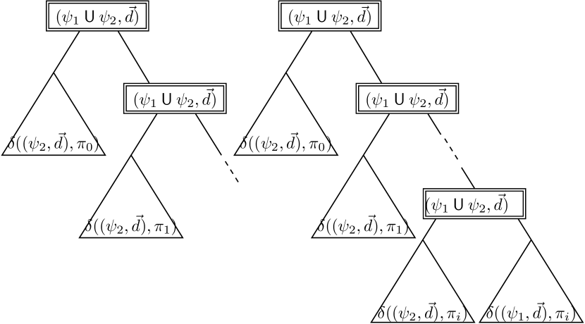
• If $\tau$ is of the form in Fig. 4 on the left, its utility $\min_{\rho\in\mathop{\mathrm{path}}\nolimits(\tau)}F^{\infty}(\rho)$ is $\inf_{j\in\mathbb{N}}\mathcal{L}(\mathcal{A}_{\varphi,\varepsilon}^{(\psi_{2},\vec{d})})(\pi^{j})$; note that the rightmost path’s value of $F^{\infty}$ is $1$ and hence does not appear here.

• If $\tau$ is of the form in Fig. 4 on the right, its utility $\min_{\rho\in\mathop{\mathrm{path}}\nolimits(\tau)}F^{\infty}(\rho)$ is given by $\min\bigl{\{}\,\mathcal{L}(\mathcal{A}_{\varphi,\varepsilon}^{(\psi_{1},\vec{d})})(\pi^{i}),\,\min_{0\leq j\leq i}\mathcal{L}(\mathcal{A}_{\varphi,\varepsilon}^{(\psi_{2},\vec{d})})(\pi^{j})\,\bigr{\}}$ where $i$ is the depth of the last occurrence of the node $(\psi_{1}\mathbin{\mathsf{U}}\psi_{2},\vec{d})$.

The value $\mathcal{L}(\mathcal{A}_{\varphi,\varepsilon}^{(\psi_{1}\mathbin{\mathsf{U}}\psi_{2},\vec{d})})(\pi)$ is defined as the supremum of these utilities. Therefore:

$$\mathcal{L}(\mathcal{A}_{\varphi,\varepsilon}^{(\psi_{1}\mathbin{\mathsf{U}}\psi_{2},\vec{d})})(\pi)$$

$$=\max\bigl{\{}\,\sup_{i\in\mathbb{N}}\bigl{(}\;\min\bigl{\{}\,\mathcal{L}(\mathcal{A}_{\varphi,\varepsilon}^{(\psi_{1},\vec{d})})(\pi^{i}),\,\max_{0\leq j\leq i}\mathcal{L}(\mathcal{A}_{\varphi,\varepsilon}^{(\psi_{2},\vec{d})})(\pi^{j})\,\bigr{\}}\;\bigr{)},\;\inf_{j\in\mathbb{N}}\mathcal{L}(\mathcal{A}_{\varphi,\varepsilon}^{(\psi_{2},\vec{d})})(\pi^{j})\,\bigr{\}}$$

$$\in\left[\begin{array}[]{r}\displaystyle\max\bigl{\{}\,\sup_{j\in\mathbb{N}}\bigl{(}\;\min\bigl{\{}\,\vec{d}\boxtimes\llbracket\pi^{j},\psi_{1}\rrbracket,\,\min_{0\leq i\leq j}\vec{d}\boxtimes\llbracket\pi^{i},\psi_{2}\rrbracket\,\bigr{\}}\;\bigr{)}\;,\inf_{i\in\mathbb{N}}\vec{d}\boxtimes\llbracket\pi^{i},\psi_{2}\rrbracket\,\bigr{\}}-\varepsilon\,,\phantom{hoge}\\ \displaystyle\max\bigl{\{}\,\sup_{j\in\mathbb{N}}\bigl{(}\;\min\bigl{\{}\,\vec{d}\boxtimes\llbracket\pi^{j},\psi_{1}\rrbracket,\,\min_{0\leq i\leq j}\vec{d}\boxtimes\llbracket\pi^{i},\psi_{2}\rrbracket\,\bigr{\}}\;\bigr{)}\;,\inf_{i\in\mathbb{N}}\vec{d}\boxtimes\llbracket\pi^{i},\psi_{2}\rrbracket\,\bigr{\}}\end{array}\right]$$

by the induction hypothesis

$$=\bigl{[}\,\vec{d}\boxtimes\llbracket\pi,\psi_{1}\mathbin{\mathsf{U}}\psi_{2}\rrbracket-\varepsilon\,,\;\vec{d}\boxtimes\llbracket\pi,\psi_{1}\mathbin{\mathsf{U}}\psi_{2}\rrbracket\,\bigr{]}\qquad\text{by\leavevmode\nobreak\ (\ref{eq:actionIsAntiMonotoneAndConti}),}$$

concluding the case when $\psi=\psi_{1}\mathbin{\mathsf{U}}\psi_{2}$ and $|\vec{d}|$ is even.

Suppose that $\psi=\psi_{1}\mathbin{\mathsf{U}}_{\eta^{+k}}\psi_{2}$ and that ${|\vec{d}|}$ is odd. We prove the claim by induction on $k$, going backwards, decrementing $k$ starting from the event horizon towards $k=0$. As the base case, assume that $k$ is big enough and we are beyond the event horizon, that is, $\eta(k)\cdot\prod_{i=1}^{n}d_{i}\leq\varepsilon$. Let $\pi\in(\mathcal{P}(\mathit{AP}))^{\omega}$ and $\vec{d}=d_{1}\dotsc d_{n}$. Then we have $\llbracket\pi,\psi\rrbracket\cdot\prod_{i=0}^{n}d_{i}=\llbracket\pi,\psi_{1}\mathbin{\mathsf{U}}_{\eta^{+k}}\psi_{2}\rrbracket\cdot\prod_{i=0}^{n}d_{i}\leq\varepsilon$, by Lem. 2.6 and that $\eta^{+k}(0)=\eta(k)$. It follows from (8) that we have $0\leq\vec{d}\boxtimes\llbracket\pi,\psi\rrbracket-\vec{d}\boxtimes 0\leq\varepsilon$ (note that $n=|\vec{d}|$ is odd). Therefore

$$\mathcal{L}(\mathcal{A}_{\varphi,\varepsilon}^{(\psi_{1}\mathbin{\mathsf{U}}_{\eta^{+k}}\psi_{2},\vec{d})})(\pi) =\vec{d}\boxtimes 0\qquad\text{by\leavevmode\nobreak\ (\ref{eq:defDeltaBeyondEventHorizon})}$$

$$\in\bigl{[}\,\vec{d}\boxtimes\llbracket\pi,\psi\rrbracket-\varepsilon,\,\vec{d}\boxtimes\llbracket\pi,\psi\rrbracket\,\bigr{]}\enspace.$$

Now, as the step case, assume that $\eta(k)\cdot\prod_{i=1}^{n}d_{i}>\varepsilon$ and that the claim has been shown for $k+1$. The analogue below of $\psi_{1}\mathbin{\mathsf{U}}\psi_{2}\cong\psi_{2}\lor\bigl{(}\psi_{1}\land\mathsf{X}(\psi_{1}\mathbin{\mathsf{U}}\psi_{2})\bigr{)}$ follows easily from Def. 2.5:

$$\llbracket\pi,\psi_{1}\mathbin{\mathsf{U}}_{\eta^{+k}}\psi_{2}\rrbracket\;=\;\max\bigl{\{}\,\eta^{+k}(0)\cdot\llbracket\pi,\psi_{2}\rrbracket,\,\min\bigl{\{}\,\eta^{+k}(0)\cdot\llbracket\pi,\psi_{1}\rrbracket,\,\llbracket\pi^{1},\psi_{1}\mathbin{\mathsf{U}}_{\eta^{+(k+1)}}\psi_{2}\rrbracket\,\bigr{\}}\,\bigr{\}}\enspace.$$

Therefore

$$\vec{d}\boxtimes\llbracket\pi,\psi_{1}\mathbin{\mathsf{U}}_{\eta^{+k}}\psi_{2}\rrbracket$$ (36)

$$=\max\bigl{\{}\,\vec{d}\boxtimes\bigl{(}\eta^{+k}(0)\cdot\llbracket\pi,\psi_{2}\rrbracket\bigr{)},\,$$

$$\qquad\min\bigl{\{}\,\vec{d}\boxtimes\bigl{(}\eta^{+k}(0)\cdot\llbracket\pi,\psi_{1}\rrbracket\bigr{)},\,\vec{d}\boxtimes\llbracket\pi^{1},\psi_{1}\mathbin{\mathsf{U}}_{\eta^{+(k+1)}}\psi_{2}\rrbracket\,\bigr{\}}\,\bigr{\}}$$

$$=\max\bigl{\{}\,\bigl{(}\vec{d}\odot\eta^{+k}(0)\bigr{)}\boxtimes\llbracket\pi,\psi_{2}\rrbracket,\,$$

$$\qquad\min\bigl{\{}\,\bigl{(}\vec{d}\odot\eta^{+k}(0)\bigr{)}\boxtimes\llbracket\pi,\psi_{1}\rrbracket,\,\vec{d}\boxtimes\llbracket\pi^{1},\psi_{1}\mathbin{\mathsf{U}}_{\eta^{+(k+1)}}\psi_{2}\rrbracket\,\bigr{\}}\,\bigr{\}}\enspace,$$

where the first equality is due to the monotonicity of $\vec{d}\boxtimes(\underline{\phantom{n}}\,)$, and the second is by (9). Now

$$\mathcal{L}(\mathcal{A}_{\varphi,\varepsilon}^{(\psi_{1}\mathbin{\mathsf{U}}_{\eta^{+k}}\psi_{2},\vec{d})})(\pi)$$

$$=\max\bigl{\{}\,\mathcal{L}(\mathcal{A}_{\varphi,\varepsilon}^{(\psi_{2},\vec{d}\odot\eta^{+k}(0))})(\pi),\,\min\bigl{\{}\,\mathcal{L}(\mathcal{A}_{\varphi,\varepsilon}^{(\psi_{1},\vec{d}\odot\eta^{+k}(0))})(\pi),\,\mathcal{L}(\mathcal{A}_{\varphi,\varepsilon}^{(\psi_{1}\mathbin{\mathsf{U}}_{\eta^{+(k+1)}}\psi_{2},\vec{d})})(\pi^{1})\,\bigr{\}}\,\bigr{\}}$$

by Def. 4.7. By the induction hypothesis (the claim has been shown for simpler formulas as well as $\psi_{1}\mathbin{\mathsf{U}}_{\eta^{+(k+1)}}\psi_{2}$), a lower bound of the above value is given by

$$\max\Bigl{\{}\,\Bigl{(}\bigl{(}\vec{d}\odot\eta^{+k}(0)\bigr{)}\boxtimes\llbracket\pi,\psi_{2}\rrbracket\Bigr{)}-\varepsilon,\,$$

$$\qquad\min\Bigl{\{}\,\Bigl{(}\bigl{(}\vec{d}\odot\eta^{+k}(0)\bigr{)}\boxtimes\llbracket\pi,\psi_{1}\rrbracket\Bigr{)}-\varepsilon,\,\Bigl{(}\vec{d}\boxtimes\llbracket\pi^{1},\psi_{1}\mathbin{\mathsf{U}}_{\eta^{+(k+1)}}\psi_{2}\rrbracket\Bigr{)}-\varepsilon\,\Bigr{\}}\,\Bigr{\}}$$

$$=\vec{d}\boxtimes\llbracket\pi,\psi_{1}\mathbin{\mathsf{U}}_{\eta^{+k}}\psi_{2}\rrbracket-\varepsilon\qquad\text{by\leavevmode\nobreak\ (\ref{eq:201410152355}).}$$

Similarly an upper bound $\vec{d}\boxtimes\llbracket\pi,\psi_{1}\mathbin{\mathsf{U}}_{\eta^{+k}}\psi_{2}\rrbracket$ is obtained by the induction hypothesis and (36). This proves the claim.

The remaining case where $\psi=\psi_{1}\mathbin{\mathsf{U}}_{\eta^{+k}}\psi_{2}$ and ${|\vec{d}|}$ is even is similar to the last case. We describe only the base case of induction, where $k$ is big enough so that $\eta(k)\cdot\prod_{i=1}^{n}d_{i}\leq\varepsilon$. By Lem. 2.6 we have $\llbracket\pi,\psi\rrbracket\in[0,\eta^{k}(0)]$; therefore

$$\textstyle 0\;\leq\;\eta(k)-\llbracket\pi,\psi\rrbracket\;\leq\;\eta(k)\;\leq\;\varepsilon/\prod_{i=1}^{n}d_{i}\enspace.$$

By (8) and that $n$ is even, we have

$$\vec{d}\boxtimes\llbracket\pi,\psi\rrbracket-\vec{d}\boxtimes\eta(k)\; =\;\bigl{(}\prod_{i=1}^{n}d_{i}\bigr{)}\cdot\bigl{(}\,\eta(k)-\llbracket\pi,\psi\rrbracket\,\bigr{)}\;\in\;[0,\varepsilon]\enspace.$$

Hence

$$\mathcal{L}(\mathcal{A}_{\varphi,\varepsilon}^{(\psi_{1}\mathbin{\mathsf{U}}_{\eta^{+k}}\psi_{2},\vec{d})})(\pi) =\vec{d}\boxtimes\eta(k)\qquad\text{by\leavevmode\nobreak\ (\ref{eq:defDeltaBeyondEventHorizon})}$$

$$\in\bigl{[}\,\vec{d}\boxtimes\llbracket\pi,\psi\rrbracket-\varepsilon,\,\vec{d}\boxtimes\llbracket\pi,\psi\rrbracket\,\bigr{]}\enspace.$$

This concludes the proof. ∎

B.5. Proof of Lem. 4.12

Proof.

It follows easily from the definition that there is a bijective correspondence between: a run $\zeta=(q^{\prime}_{0},s^{\prime}_{0})\,\bullet\,(q^{\prime}_{1},s^{\prime}_{1})\,\bullet\,\dotsc$ of $\mathcal{A}\times\mathcal{K}$; and a pair $(\xi,\rho)$ of a path $\xi=s^{\prime}_{0}s^{\prime}_{1}\dotsc\in\mathop{\mathrm{path}}\nolimits(\mathcal{K})$ of $\mathcal{K}$ and a run $\rho$ over $\lambda(\xi)$ of $\mathcal{A}$. Moreover, the acceptance value of $\zeta$ in $\mathcal{A}\times\mathcal{K}$ is equal to that of $\rho$ in $\mathcal{A}$. The claim follows immediately. ∎

B.6. Proof of Thm. 4.13

Proof.

$$\llbracket s_{0}s_{1}\dotsc,\varphi\rrbracket\; \geq\;\mathcal{L}(\mathcal{A}^{\mathrm{na}}_{\varphi,\varepsilon})\bigl{(}\,\lambda(s_{0})\lambda(s_{1})\dotsc\,\bigr{)}\qquad\text{by Cor.\leavevmode\nobreak\ \ref{cor:NBAforLTL}}$$

$$=\;\max_{\xi\in\mathop{\mathrm{path}}\nolimits(\mathcal{K})}\mathcal{L}(\mathcal{A}^{\mathrm{na}}_{\varphi,\varepsilon})\bigl{(}\,\lambda(\xi)\,\bigr{)}\qquad\text{by Lem.\leavevmode\nobreak\ \ref{lem:fromOptimalInATimesKToOptimalInA}}$$

$$\geq\;\sup_{\xi\in\mathop{\mathrm{path}}\nolimits(\mathcal{K})}\llbracket\xi,\varphi\rrbracket-\varepsilon\qquad\text{by Cor.\leavevmode\nobreak\ \ref{cor:NBAforLTL}.}$$

The solution $s_{0}s_{1}\dotsc$ thus obtained arises from a lasso computation of $\mathcal{A}^{\mathrm{na}}_{\varphi,\varepsilon}\times\mathcal{K}$ (by the algorithm in Lem. 3.2), hence is ultimately periodic. ∎

B.7. Proof of Prop. 4.15

Proof.

In the proof of Lem. A.1, we construct $\mathcal{A}_{\varphi,\varepsilon}^{\vec{d}}$ inductively. We shall therefore prove, inductively on the construction on $\varphi$, that the size of the state space of $\mathcal{A}_{\varphi,\varepsilon}^{\vec{d}}$ is singly exponential in $|\langle\varphi\rangle|$ and in the length of the description of $\varepsilon$.

In the case where $\varphi=\mathtt{True},p,\varphi_{1}\land\varphi_{2},\lnot\varphi^{\prime},\mathsf{X}\varphi^{\prime}$ or $\varphi_{1}\mathbin{\mathsf{U}}\varphi_{2}$, the claim is obvious.

Suppose that $\varphi=\varphi_{1}\mathbin{\mathsf{U}}_{\mathrm{exp}_{\lambda}^{+k}}\varphi_{2}$ where $\lambda\in(0,1)$. Let $k_{\max}=\lceil\log_{\lambda}\varepsilon\rceil+1$. Recall that the construction of $\mathcal{A}_{\varphi_{1}\mathbin{\mathsf{U}}_{\mathrm{exp}_{\lambda}^{+k}}\varphi_{2},\varepsilon}^{\vec{d}}$ in Lem. A.1 is by backward induction on $k$, from $k=k_{\max}$ to $k=0$. In the base case when $k=k_{\max}$, we have $\mathrm{exp}_{\lambda}^{+k}(0)\leq\varepsilon$ (beyond the event horizon); in this case the size of the state space of $\mathcal{A}_{\varphi,\varepsilon}^{\vec{d}}$ is one. In the step case, the state space of $\mathcal{A}_{\varphi_{1}\mathbin{\mathsf{U}}_{\mathrm{exp}_{\lambda}^{+k}}\varphi_{2},\varepsilon}^{\vec{d}}$ is the union of: those of the two automata for $\varphi_{1}$ and $\varphi_{2}$; that of the automaton $\mathcal{A}_{\varphi_{1}\mathbin{\mathsf{U}}_{\mathrm{exp}_{\lambda}^{+(k+1)}}\varphi_{2},\varepsilon}^{\vec{d}}$; and the singleton of the initial state of $\mathcal{A}_{\varphi,\varepsilon}^{\vec{d}}$. Overall, the state space of $\mathcal{A}_{\varphi_{1}\mathbin{\mathsf{U}}_{\mathrm{exp}_{\lambda}^{+k}}\varphi_{2},\varepsilon}^{\vec{d}}$ increases as $k$ decreases, and the maximum is when $k=0$—in which case the state space of $\mathcal{A}_{\varphi_{1}\mathbin{\mathsf{U}}_{\mathrm{exp}_{\lambda}}\varphi_{2},\varepsilon}^{\vec{d}}$ is roughly $\mathcal{O}(k_{\max})=\mathcal{O}(\lceil\log_{\lambda}\varepsilon\rceil+1)$ copies of those of the two automata for $\varphi_{1}$ and $\varphi_{2}$. Now we appeal to the fact used in [3] that the value $k_{\max}\sim\log_{\lambda}\varepsilon=\log\varepsilon/\log\lambda$ is polynomial in the length of the description of $\lambda$—hence in $|\langle\varphi\rangle|$—and $\varepsilon$. By this fact and the induction hypothesis, the size of the state space of $\mathcal{A}_{\varphi,\varepsilon}^{\vec{d}}$ is singly exponential in $|\langle\varphi\rangle|$ and in the length of the description of $\varepsilon$.

Suppose that $\varphi=\varphi_{1}\oplus\varphi_{2}$. Since $(\vec{d}\boxtimes v_{1}-\varepsilon)\oplus(\vec{d}\boxtimes v_{2}-\varepsilon)=\vec{d}\boxtimes(v_{1}\oplus v_{2})-\varepsilon$, we have $\mathcal{A}_{\varphi,\varepsilon}^{\vec{d}}$ coincide with $\mathcal{A}_{\varphi_{1},\varepsilon}^{\vec{d}}\oplus\mathcal{A}_{\varphi_{2},\varepsilon}^{\vec{d}}$—where the latter is defined in Prop. 3.5. (We note that the construction in Prop. 3.5 can be readily adapted to alternating $[0,1]$-acceptance automata, too.) Hence the size of the state space of $\mathcal{A}_{\varphi,\varepsilon}^{\vec{d}}$ is polynomial in those of $\mathcal{A}_{\varphi_{1},\varepsilon}^{\vec{d}}$ and $\mathcal{A}_{\varphi_{2},\varepsilon}^{\vec{d}}$. By the induction hypothesis, the size of the state space of $\mathcal{A}_{\varphi,\varepsilon}^{\vec{d}}$ is singly exponential in $|\langle\varphi\rangle|$ and in the length of the description of $\varepsilon$. ∎

B.8. Proof of Thm. 4.16

Proof.

The construction in Prop. 3.4 (from $\mathcal{A}_{\varphi,\varepsilon}$ to $\mathcal{A}^{\mathrm{na}}_{\varphi,\varepsilon}$) results in $\mathcal{A}^{\mathrm{na}}_{\varphi,\varepsilon}$ that is exponentially bigger than $\mathcal{A}_{\varphi,\varepsilon}$; the size of the product $\mathcal{A}^{\mathrm{na}}_{\varphi,\varepsilon}\times\mathcal{K}$ (Def. 4.11) is linear in those of $\mathcal{A}^{\mathrm{na}}_{\varphi,\varepsilon}$ and $\mathcal{K}$; and finding an optimal run by Lem. 3.2 is in NLOGSPACE. Combined with Prop. 4.15, the overall complexity is EXPSPACE in $|\langle\varphi\rangle|$ and NLOGSPACE in the size of $\mathcal{K}$. ∎

B.9. Proof of Thm. 4.17

Firstly we give an alternative proof to the following statement (that is a restriction of Prop. 4.15). It is used in the proof of Thm. 4.17.

Sublemma B.2 (size of $\mathcal{A}_{\varphi,\varepsilon}$, for $\textrm{LTL}^{\mathrm{disc}}[\mathcal{D}_{\mathrm{exp}},\emptyset]$).

Let $\varphi$ be an $\textrm{LTL}^{\mathrm{disc}}[\mathcal{D}_{\mathrm{exp}},\emptyset]$ formula and $\varepsilon\in(0,1)\cap\mathbb{Q}$ be a positive rational number. The size of the state space of the alternating $[0,1]$-acceptance automaton $\mathcal{A}_{\varphi,\varepsilon}$ is singly exponential in $|\langle\varphi\rangle|$ and in the length of the description of $\varepsilon$. ∎

Proof.

(Of Sublem. B.2) Recall that a state of $\mathcal{A}_{\varphi,\varepsilon}$ is a pair $(\psi,\vec{d})$ of $\psi\in\mathit{xcl}(\varphi)$ and $\vec{d}\in[0,1]^{+}$. We first claim that the number of different $\psi$’s is polynomial in $|\langle\varphi\rangle|$ and $\log\varepsilon$. The claim is obvious except for the number of the formulas $\psi$ of the form $\psi_{1}\mathbin{\mathsf{U}}_{\eta^{+i}}\psi_{2}$, for varying $i\in\mathbb{N}$. Let $\lambda_{0}$ be the maximum number in $\varphi$ used as the base of an exponential discounting function. For each subformula $\psi_{1}\mathbin{\mathsf{U}}_{\eta}\psi_{2}$ of $\varphi$, the numbers $i$ for which we have a state $\bigl{(}\,\psi_{1}\mathbin{\mathsf{U}}_{\eta^{+i}}\psi_{2},\vec{d}\,\bigr{)}$ in $\mathcal{A}_{\varphi,\varepsilon}$ is bounded by $1+\lceil\log_{\lambda_{0}}\varepsilon\rceil$. Now we appeal to the fact used in [3] that the value $\log_{\lambda_{0}}\varepsilon=\log\varepsilon/\log\lambda_{0}$ is polynomial in the length of the description of $\lambda_{0}$—hence in $|\langle\varphi\rangle|$—and $\varepsilon$.

Our second claim is that the number of different $\vec{d}$’s occurring in states of $\mathcal{A}_{\varphi,\varepsilon}$ is exponential in $|\langle\varphi\rangle|$ and the description length of $\varepsilon$, hence is the bottleneck in complexity. The length of a discount sequence $\vec{d}$ is bounded by the number of negations in $\varphi$, therefore by $|\langle\varphi\rangle|$. Each entry $d_{i}$ is a multiple $\lambda_{i_{1}}\lambda_{i_{2}}\dotsc\lambda_{i_{m}}$ of different discounting bases $\lambda_{j}$ (there are at most $|\langle\varphi\rangle|$-many such), and since its value must be bigger than $\varepsilon$, the length $m$ of such a multiple is at most $\log_{\lambda_{0}}\varepsilon$. Therefore the number of candidates for $d_{i}=\lambda_{i_{1}}\lambda_{i_{2}}\dotsc\lambda_{i_{m}}$ is bounded by $|\langle\varphi\rangle|^{\log_{\lambda_{0}}\varepsilon}$; appealing to the fact (see [3]) that $\log_{\lambda}\varepsilon=\log\varepsilon/\log\lambda$ is polynomial in the length of the description of $\lambda$ and $\varepsilon$, we obtain the claim. ∎

Proof.

(Of Thm. 4.17, sketch) We describe how to avoid the exponential blowup in the translation from $\mathcal{A}_{\varphi,\varepsilon}$ to $\mathcal{A}^{\mathrm{na}}_{\varphi,\varepsilon}$.

Looking at the construction of Prop. 3.4 in case of $\mathcal{A}=\mathcal{A}_{\varphi,\varepsilon}$, we have $V_{Q}=\{0,1\}$, therefore

$$Q^{\prime}\;=\;{\mathcal{P}(Q\times 2)}\times V_{\delta}\times 2\;\cong\;\bigl{(}\mathcal{P}(Q)\bigr{)}^{2}\times V_{\delta}\times 2\enspace.$$ (37)

Here the original state space $Q$ is bounded by $\mathit{xcl}_{\varepsilon}(\varphi)\times|\langle\varphi\rangle|^{\log_{\lambda_{0}}\varepsilon}$, where

$$\mathit{xcl}_{\varepsilon}(\varphi)\;=\;\mathit{xcl}(\varphi)\setminus\{\varphi_{1}\mathbin{\mathsf{U}}_{\eta}\varphi_{2}\in\mathit{xcl}(\varphi)\mid\eta(0)<\varepsilon\}$$

is a finite set and the second component $|\langle\varphi\rangle|^{\log_{\lambda_{0}}\varepsilon}$ is from the proof of Prop. B.2.

The optimization lies in the reduction of $\mathcal{P}(Q)$ that occurs in (37) to

$$\bigl{(}(Q\times Q^{2}\times Q^{2})\cup\{\bullet\}\bigr{)}^{\mathit{xcl}_{\varepsilon}(\varphi)}\enspace,$$ (38)

hence from a double exponential to a single exponential; recall from the proof of Prop. B.2 that $Q$ is exponential and $\mathit{xcl}_{\varepsilon}(\varphi)$ is polynomial, in $|\langle\varphi\rangle|$ and the description length of $\varepsilon$.

The reduction is done concretely as follows. Given a set

$$\bigl{\{}\,(\psi,\vec{d_{1}}),\,(\psi,\vec{d_{2}}),\,\dotsc,(\psi,\vec{d_{m}})\,\bigr{\}}$$ (39)

of states of $Q$ with a common first component $\psi$, we suppress the set into the function

$$(\vec{d_{1}}\land\cdots\land\vec{d_{m}})\boxtimes(\underline{\phantom{n}}\,)\;\colon\;v\;\longmapsto\;\min\{\vec{d_{1}}\boxtimes v,\cdots,\vec{d_{m}}\boxtimes v\}\$$ (40)

that does the same job. The latter is a piecewise linear function on $[0,1]$ and hence is presented as a disjunction of pairs $(f_{i},[l_{i},r_{i}])$ of a linear function $f_{i}$ and its domain (here $l_{i},r_{i}\in(0,1)$). Now $f_{i}$ is represented by some discount sequence so there are at most $|Q|$-many of them. A point $l_{i}\in[0,1]$ is expressed as the cross point of two linear functions, each represented by a discount sequence. The same goes for $r_{i}$. Moreover, disjunction is taken out of a single state in the resulting automaton—from alternating to non-alternating we only need to bundle up states in conjunction. In summary, to express the piecewise linear function in (40) we need: $Q$ to represent $f_{i}$; $Q^{2}$ to represent $l_{i}$; and $Q^{2}$ to represent $r_{i}$, resulting in $Q\times Q^{2}\times Q^{2}$ in (38).

We consider all those sets in the form of (39), therefore we need $Q\times Q^{2}\times Q^{2}$ for each formula $\psi\in\mathit{xcl}_{\varepsilon}(\varphi)$. The set $\{\bullet\}$ is in (38) to take care of the case when the set (39) for the formula $\psi$ is empty. ∎

Appendix C Reduction of Fuzzy Automata to $[0,1]$-Acceptance Automata

A generalization of $[0,1]$-acceptance automaton is naturally obtained by making transitions also $[0,1]$-weighted. The result is called fuzzy automaton and studied e.g. in [20]. Here we show that this generalization does not add expressivity. In fact we prove a more general result, parametrizing $[0,1]$ into a general semiring $\mathbb{K}$ (under certain conditions).

We follow [13] and impose certain conditions on a semiring $K$ of weights.

Definition C.1 ([13]).

A tuple $\mathbb{K}=(K,\leq,+,\cdot,0,1)$ is called an ordered semiring if $(K,+,\cdot,0,1)$ is a semiring, $(K,\leq)$ is a partially ordered set and both $+$ and $\cdot$ are monotonic.

An ordered semiring $\mathbb{K}=(K,\leq,+,\cdot,0,1)$ is said to be lattice-complete if: $(K,\leq)$ is a complete lattice; the units $0,1$ of $+,\cdot$ satisfy $0\leq x\leq 1$ for each $x\in K$; and

$$y+\sup_{i\in I}x_{i}\;=\;\sup_{i\in I}(y+x_{i})$$

for each family $(x_{i})_{i\in I}$ and each $y\in K$. We define an infinite sum, as usual, by

$$\sum_{i\in I}x_{i}\;=\;\sup_{F\in{\mathcal{P}_{\mathrm{fin}}}(I)}\sum_{i\in F}x_{i}$$

where ${\mathcal{P}_{\mathrm{fin}}}(I)$ is the set of finite subsets of $I$.

A semiring is locally finite if the underlying monoid $(K,\cdot,1)$ is locally finite, that is: for each finite subset $F\subseteq K$, the submonoid of $(K,\cdot,1)$ generated by $F$ is finite.

The notion of $\mathbb{K}$-weighted (Büchi) automaton is studied in [13], from which the following definition is taken.

Definition C.2 ($\mathbb{K}$-acceptance (Büchi) automaton, $\mathbb{K}$-weighted (Büchi) automaton).

Let $(K,\leq,+,\cdot,0,1)$ be a lattice-complete semiring. A $\mathbb{K}$-acceptance (Büchi) automaton is a tuple $\mathcal{A}=(\Sigma,Q,I,\delta,F)$, where $\Sigma$ is a finite alphabet, $Q$ is a finite set of states, $I\subseteq Q$ is a set of initial states, $\delta:Q\times\Sigma\rightarrow\mathcal{P}(Q)$ is a transition function and $F:Q\rightarrow K$ is a function that assigns an acceptance value to each state. We define the language $\mathcal{L}(\mathcal{A}):\Sigma^{\omega}\rightarrow K$ of $\mathcal{A}$ as

$$\mathcal{L}(\mathcal{A})(w)=\sum_{\rho\in\mathop{\mathrm{run}}\nolimits(w)}\max\{F(q)\mid q\in\mathrm{Inf}(\rho)\}\enspace.$$

A $\mathbb{K}$-weighted (Büchi) automaton is a tuple $\mathcal{A}=(\Sigma,Q,I,\delta,F)$, where $\Sigma$ is a finite alphabet, $Q$ is a finite set of states, $I:Q\rightarrow K$ is a function assigns an initial weight to each state, $\delta:Q\times\Sigma\rightarrow{K}^{Q}$ is a ($\mathbb{K}$-weighted) transition function and $F:Q\rightarrow K$ is a function assigns an acceptance value to each state. We define the language $\mathcal{L}(\mathcal{A}):\Sigma^{\omega}\rightarrow K$ of $\mathcal{A}$ by

$$\mathcal{L}(\mathcal{A})(w)=\sum_{q_{0}q_{1}\ldots\in Q^{\omega}}\inf_{n\in\mathbb{N}}\sup_{i\geq n}\bigl{(}\,I(q_{0})\cdot\delta(q_{0},w_{0})(q_{1})\cdot\,\cdots\,\cdot\delta(q_{i-1},w_{i-1})(q_{i})\cdot F(q_{i})\,\bigr{)}\enspace.$$

These notions specialize to $[0,1]$-acceptance automaton and fuzzy automaton [20] by taking the fuzzy semiring $([0,1],\max,\min,0,1)$ as $\mathbb{K}$ in the above definitions.

Locally finiteness of a semiring [13] is central in the following result. Its proof is not hard but the result is not explicit in [13] or elsewhere.

Lemma C.3.

Let $\mathbb{K}=(K,\leq,+,\cdot,0,1)$ be a lattice-complete semiring and $\mathcal{A}=(\Sigma,Q,I,\delta,F)$ be a $\mathbb{K}$-weighted automaton. If $\mathbb{K}$ is locally finite (Def. C.1), there exists a $\mathbb{K}$-acceptance automaton $\mathcal{A}^{\prime}=(\Sigma,Q^{\prime},I^{\prime},\delta^{\prime},F^{\prime})$ such that $\mathcal{L}(\mathcal{A})=\mathcal{L}(\mathcal{A}^{\prime})$.

Proof.

Let $(F,\cdot,1)$ be the submonoid of $(K,\cdot,1)$ generated by the (finite) set of weights of transitions occurring in $\mathcal{A}$, that is, $\{\delta(q,a)(q^{\prime})\mid q,q^{\prime}\in Q,a\in\Sigma\}$. The set $F$ is finite since $\mathbb{K}$ is locally finite. We now define $\mathcal{A}^{\prime}=(\Sigma,Q^{\prime},I^{\prime},\delta^{\prime},F^{\prime})$ as follows.

$$Q^{\prime} =Q\times F\enspace, I^{\prime} =I\times\{1\}\enspace,$$

$$\delta^{\prime}\bigl{(}\,(q,k),\,a\,\bigr{)} =\bigl{\{}\;\bigl{(}\,q^{\prime},\;k\cdot\delta(q,a)(q^{\prime})\,\bigr{)}\;\bigl{|}\bigr{.}\;q^{\prime}\in Q\;\bigr{\}}\enspace, F^{\prime}(q,k) =k\cdot F(q)\enspace.$$

The proof of $\mathcal{L}(\mathcal{A})=\mathcal{L}(\mathcal{A}^{\prime})$ is straightforward. ∎

It is straightforward that the fuzzy semiring $([0,1],\max,\min,0,1)$ is locally finite. This leads to:

Corollary C.4.

Let $\mathcal{A}$ be a fuzzy automaton. There exists a $[0,1]$-acceptance automaton $\mathcal{A}^{\prime}$ such that $\mathcal{L}(\mathcal{A})=\mathcal{L}(\mathcal{A}^{\prime})$. ∎

The main results of [20, 13] concern the characterization of so-called $\omega$-rational formal power series over $\mathbb{K}$—those which are generated by $\omega$-regular-like expressions—by $\mathbb{K}$-weighted Büchi automata. Lem. C.3 therefore gives us another characterization by $\mathbb{K}$-acceptance Büchi automata.

References

- [1] Yasmina Abdeddaïm, Eugene Asarin, and Oded Maler. Scheduling with timed automata. Theor. Comput. Sci., 354(2):272–300, 2006.
- [2] Shaull Almagor, Udi Boker, and Orna Kupferman. Formalizing and reasoning about quality. In Fedor V. Fomin, Rusins Freivalds, Marta Z. Kwiatkowska, and David Peleg, editors, Automata, Languages, and Programming - 40th International Colloquium, ICALP 2013, Riga, Latvia, July 8-12, 2013, Proceedings, Part II, volume 7966 of Lecture Notes in Computer Science, pages 15–27. Springer, 2013.
- [3] Shaull Almagor, Udi Boker, and Orna Kupferman. Discounting in LTL. In Erika Ábrahám and Klaus Havelund, editors, Tools and Algorithms for the Construction and Analysis of Systems - 20th International Conference, TACAS 2014, Held as Part of the European Joint Conferences on Theory and Practice of Software, ETAPS 2014, Grenoble, France, April 5-13, 2014. Proceedings, volume 8413 of Lecture Notes in Computer Science, pages 424–439. Springer, 2014.
- [4] Shaull Almagor, Udi Boker, and Orna Kupferman. Formalizing and reasoning about quality. Extended version of [2], preprint (private communication), 2014.
- [5] Christel Baier, Clemens Dubslaff, and Sascha Klüppelholz. Trade-off analysis meets probabilistic model checking. In Thomas A. Henzinger and Dale Miller, editors, Joint Meeting of the Twenty-Third EACSL Annual Conference on Computer Science Logic (CSL) and the Twenty-Ninth Annual ACM/IEEE Symposium on Logic in Computer Science (LICS), CSL-LICS ’14, Vienna, Austria, July 14 - 18, 2014, page 1. ACM, 2014.
- [6] Roderick Bloem, Krishnendu Chatterjee, Thomas A. Henzinger, and Barbara Jobstmann. Better quality in synthesis through quantitative objectives. In Ahmed Bouajjani and Oded Maler, editors, Computer Aided Verification, 21st International Conference, CAV 2009, Grenoble, France, June 26 - July 2, 2009. Proceedings, volume 5643 of Lecture Notes in Computer Science, pages 140–156. Springer, 2009.
- [7] Patricia Bouyer, Nicolas Markey, and Raj Mohan Matteplackel. Averaging in LTL. In Paolo Baldan and Daniele Gorla, editors, CONCUR 2014 - Concurrency Theory - 25th International Conference, CONCUR 2014, Rome, Italy, September 2-5, 2014. Proceedings, volume 8704 of Lecture Notes in Computer Science, pages 266–280. Springer, 2014.
- [8] Pavol Cerný, Krishnendu Chatterjee, Thomas A. Henzinger, Arjun Radhakrishna, and Rohit Singh. Quantitative synthesis for concurrent programs. In Ganesh Gopalakrishnan and Shaz Qadeer, editors, Computer Aided Verification - 23rd International Conference, CAV 2011, Snowbird, UT, USA, July 14-20, 2011. Proceedings, volume 6806 of Lecture Notes in Computer Science, pages 243–259. Springer, 2011.
- [9] Krishnendu Chatterjee, Laurent Doyen, and Thomas A. Henzinger. Expressiveness and closure properties for quantitative languages. Logical Methods in Computer Science, 6(3), 2010.
- [10] Krishnendu Chatterjee, Thomas A. Henzinger, and Marcin Jurdzinski. Mean-payoff parity games. In 20th IEEE Symposium on Logic in Computer Science (LICS 2005), 26-29 June 2005, Chicago, IL, USA, Proceedings, pages 178–187. IEEE Computer Society, 2005.
- [11] Ling Cheung, Mariëlle Stoelinga, and Frits W. Vaandrager. A testing scenario for probabilistic processes. J. ACM, 54(6), 2007.
- [12] Luca de Alfaro, Thomas A. Henzinger, and Rupak Majumdar. Discounting the future in systems theory. In Jos C. M. Baeten, Jan Karel Lenstra, Joachim Parrow, and Gerhard J. Woeginger, editors, Automata, Languages and Programming, 30th International Colloquium, ICALP 2003, Eindhoven, The Netherlands, June 30 - July 4, 2003. Proceedings, volume 2719 of Lecture Notes in Computer Science, pages 1022–1037. Springer, 2003.
- [13] Manfred Droste and Ulrike Püschmann. On weighted Büchi automata with order-complete weights. IJAC, 17(2):235–260, 2007.
- [14] Marco Faella, Axel Legay, and Mariëlle Stoelinga. Model checking quantitative linear time logic. Electr. Notes Theor. Comput. Sci., 220(3):61–77, 2008.
- [15] Hans Hansson and Bengt Jonsson. A logic for reasoning about time and reliability. Formal Asp. Comput., 6(5):512–535, 1994.
- [16] Orna Kupferman, Nir Piterman, and Moshe Y. Vardi. Safraless compositional synthesis. In Thomas Ball and Robert B. Jones, editors, Computer Aided Verification, 18th International Conference, CAV 2006, Seattle, WA, USA, August 17-20, 2006, Proceedings, volume 4144 of Lecture Notes in Computer Science, pages 31–44. Springer, 2006.
- [17] Orna Kupferman, Moshe Y. Vardi, and Pierre Wolper. An automata-theoretic approach to branching-time model checking. J. ACM, 47(2):312–360, March 2000.
- [18] Satoru Miyano and Takeshi Hayashi. Alternating finite automata on omega-words. Theor. Comput. Sci., 32:321–330, 1984.
- [19] Amir Pnueli and Roni Rosner. On the synthesis of a reactive module. In Conference Record of the Sixteenth Annual ACM Symposium on Principles of Programming Languages, Austin, Texas, USA, January 11-13, 1989, pages 179–190. ACM Press, 1989.
- [20] George Rahonis. Infinite fuzzy computations. Fuzzy Sets and Systems, 153(2):275–288, 2005.
- [21] R. J. van Glabbeek. The linear time–branching time spectrum I; the semantics of concrete, sequential processes. In J. A. Bergstra, A. Ponse, and S. A. Smolka, editors, Handbook of Process Algebra, chapter 1, pages 3–99. Elsevier, 2001.
- [22] Moshe Y. Vardi. An automata-theoretic approach to linear temporal logic. In Logics for Concurrency: Structure versus Automata, volume 1043 of Lecture Notes in Computer Science, pages 238–266. Springer-Verlag, 1996.
Appendix A Our General Algorithm for , Further Details