The Higgs-like boson spin from the center-edge asymmetry in the diphoton channel at the LHC

Abstract

We discuss the discrimination of the 125 GeV spin-parity $0^{+}$ Higgs-like boson observed at the LHC, decaying into two photons, $H\to\gamma\gamma$, against the hypothesis of a minimally coupled $J^{P}=2^{+}$ narrow diphoton resonance with the same mass and giving the same total number of signal events under the peak. We apply, as the basic observable of the analysis, the center-edge asymmetry $A_{\rm CE}$ of the cosine of the polar angle of the produced photons in the diphoton rest frame to distinguish between the tested spin hypotheses. We show that the center-edge asymmetry $A_{\rm CE}$ should provide strong discrimination between the possibilities of spin-0 and spin-2 with graviton-like couplings, depending on the fraction of $q\bar{q}$ production of the spin-2 signal, reaching a $\text{CL}_{s}<10^{-6}$ for $f_{qq}=0$. Indeed, the $A_{\rm CE}$ has the potential to do better than existing analyses for $f_{qq}<0.4$.

1 Introduction

In 2012 the ATLAS and CMS collaborations announced the discovery of a new 125 GeV resonance [1, 2] in their search for the Standard Model (SM) Higgs boson ($H$). It was a great triumph of the LHC experiments as in all its properties it appears just as the Higgs boson of the SM. Signals have been identified in various channels, in particular $H\rightarrow\gamma\gamma$, $H\rightarrow ZZ^{*}$ and $H\rightarrow WW^{*}$. The next step is to have precision measurements as well as determinations of the particle properties, such as its spin, $CP$, decay branching ratios, couplings with SM particles, and self-couplings.

The inclusive two-photon production process at the LHC,

$$p+p\to\gamma\gamma+X,$$ (1)

is considered a powerful testing ground for the SM, in particular as a discovery channel for Higgs boson searches. Since the observation of the Higgs-like peak by both the ATLAS and CMS experiments, much effort has been devoted to the comparison (with increased statistics) of the properties of this particle with the SM predictions for the Higgs boson, in particular to test the spin-0 character, see Refs. [3, 4, 5, 6, 7, 8] where the data sets at $\sqrt{s}=7$ and 8 TeV have been employed. In this regard, the decay channel in (1) is particularly suited, because the exchange of spin-1 is excluded, as the Landau-Yang theorem [9, 10] forbids a direct decay of an on-shell spin-1 particle into $\gamma\gamma$, and only spin-2 remains as a competitor hypothesis.

Recent measurements [4, 11, 3, 5, 6, 8] favor spin-0 over specific spin-2 scenarios. In particular, measurements of the spin of the resonance exclude a minimal coupling of the spin-2 resonance produced through gluon fusion in the $\gamma\gamma$ channel at almost $3\sigma$, and approximately at $2\sigma$ in the $ZZ$ and $WW$ channels [3].

Many proposals have been put forward to discriminate between the spin-0 and spin-2 hypotheses basically focusing on kinematic distributions, e.g, angular distributions [12, 13, 14, 15, 16, 17, 18, 19, 20, 21, 22], event shapes [23] as well as other observables [24, 25, 26, 27, 28, 29]. Among the latter, an interesting possibility to discriminate between the spin hypotheses of the Higgs-like particle was studied in [26, 28] by means of the center-edge asymmetry $A_{\rm CE}$ where its high potential as a spin discriminator was demonstrated.

The center-edge asymmetry was first proposed in [30, 32, 31] for spin identification of Kaluza-Klein gravitons at the LHC. The approach based on $A_{\rm CE}$ was further developed in subsequent papers [35, 34, 33, 36] for spin identification of heavy resonances in dilepton and diphoton channels at the LHC.

Here, we review the application of $A_{CE}$ to the angular study of the diphoton production process (1) at ATLAS extending the analysis done in [26, 28] by accounting for various admixtures of the $gg$ and $q\bar{q}$ production modes. Also, an optimization of the center-edge asymmetry on the kinematical parameter which divides the whole range of $\cos\hat{\theta}$ into center and edge regions will be performed in order to enhance the potential of $A_{CE}$ as a discriminator of spin hypotheses of Higgs-like resonances.

2 Center-edge asymmetry

The spin-2 resonance can be produced either via gluon fusion ($gg$) or via $P$-wave quark-antiquark annihilation ($q\bar{q}$). As we will show, the discrimination between the spin hypotheses is weakened if the spin-2 particle is produced predominantly via quark-antiquark annihilation.

In the diphoton decay of a Higgs-like boson, $H\to\gamma\gamma$, the spin information is extracted from the distribution in the polar angle $\hat{\theta}$ of the photons with respect to the $z$-axis of the Collins-Soper frame [37]. A scalar, spin-0, particle decays isotropically in its rest frame; before any acceptance cuts, the angular distribution $\mbox{{\rm d}}N^{\rm spin-0}/\mbox{{\rm d}}z$ ($z\equiv\cos\hat{\theta}$) is flat and the normalized distribution can be written as

$$\frac{1}{N^{\rm spin-0}}\,\frac{\mbox{{\rm d}}N^{\rm spin-0}}{\mbox{{\rm d}}z}=\frac{1}{2}.$$ (2)

The correspondence between spin and angular distribution is quite sharp: a spin-0 resonance determines a flat angular distribution, whereas spin-2 yields a quartic distribution that can be conveniently written in a self-explanatory way as [41, 42]

$$\frac{1}{N^{\rm spin-2}_{gg}}\,\frac{\mbox{{\rm d}}N^{\rm spin-2}_{gg}}{\mbox{{\rm d}}z}=\frac{5}{32}\,(1+6\,z^{2}+z^{4})$$ (3)

for the gluon fusion production mode of a spin-2 particle in a Kaluza-Klein model with minimal couplings and

$$\frac{1}{N^{\rm spin-2}_{qq}}\,\frac{\mbox{{\rm d}}N^{\rm spin-2}_{qq}}{\mbox{{\rm d}}z}=\frac{5}{8}\,(1-z^{4})$$ (4)

for the quark-antiquark annihilation. From Eqs. (3) and (4), the normalized differential distribution for a spin-2 tensor particle reads

$$\frac{1}{N^{\rm spin-2}}\,\frac{\mbox{{\rm d}}N^{\rm spin-2}}{\mbox{{\rm d}}z}=\frac{5}{32}\,(1+6\,z^{2}+z^{4})(1-f_{qq})+\frac{5}{8}\,(1-z^{4})\,f_{qq},$$ (5)

where $N^{\rm spin-2}=N^{\rm spin-2}_{gg}+N^{\rm spin-2}_{qq}$ and we denote $f_{qq}=N^{\rm spin-2}_{qq}/{N^{\rm spin-2}}$. Note that $f_{qq}$ refers to an event fraction, directly proportional to a ratio involving convolution integrals.

The background, which is dominated by the irreducible non-resonant diphoton production, turns out to be rather large before selection cuts. It is peaked in the forward and backward directions due to $t$- and $u$-channel exchange amplitudes. Determining this distribution precisely from the data is a key challenge of the analysis. Several methods have been proposed to solve that problem [26, 28, 4].

In practice the shapes in Eqs. (2) and (5) will be significantly distorted by experimental selection cuts, resolutions and contamination effects from background subtractions. However, detector cuts are not taken into account in the above Eqs. (2) and (5). We will use these expressions for illustration purposes, in order to better expose the most important features of the method we use. The final numerical results, as well as the relevant figures that will be presented in what follows refer to the full calculation, with detector cuts taken into account.

We introduce the center-edge asymmetry to quantify the separation significance between spin-0 and spin-2 resonances following the definition given in Refs. [30, 32, 31, 33, 34, 35, 36] for the case of dilepton and diphoton hadronic production:

$$A_{\rm{CE}}=\frac{N_{C}-N_{E}}{N_{C}+N_{E}}=\frac{N_{C}-N_{E}}{N},$$ (6)

where $N_{C}$ is the number of events lying within the center range $-z^{*}\leq z\leq z^{*}$ and $N_{E}$ the number of events outside this range (in the edge range). Here, $0<z^{*}<1$ is a threshold that can be optimised a priori for the best separation between spin hypotheses. For instance, in Refs. [26, 25] it is taken to be $z^{*}=0.5$. The interest of this observable should be that, being defined as a ratio between cross sections, theoretical uncertainties related to the choice of parton distributions and factorization/renormalization point should be minimized, and the same could be true, for example, of the systematic uncertanties on signal and background normalizations [26].

The formulae for $A_{\rm{CE}}$ can be easily obtained from its definition (6) and the expressions for the angular distributions (2) and (5):

$$A_{\rm CE}^{\rm spin-0}=2\,z^{*}-1,$$ (7)

and for the spin-2 case one reads

$$A_{\rm CE}^{\rm spin-2}=f_{qq}\,A_{{\rm CE},qq}^{\rm spin-2}+(1-f_{qq})\,A_{{\rm CE},gg}^{\rm spin-2},$$ (8)

where

$$A_{{\rm CE},qq}^{\rm spin-2}=\frac{1}{2}\,z^{*}\,(5-{z^{*}}^{4})-1,$$ (9)

$$A_{{\rm CE},gg}^{\rm spin-2}=\frac{5}{8}\,(z^{*}+2{z^{*}}^{3}+\frac{{z^{*}}^{5}}{5})-1.$$ (10)

To evaluate $A_{\rm CE}$ one needs the angular distributions of the diphoton events relevant to the particular experiment at the LHC. Such normalized $\cos\hat{\theta}$ distributions (simulations) were presented by ATLAS (Fig. 5 in Ref. [4]), after background subtractions and including cuts, hadronization and detector effects (which are different for the spin-0 and the spin-2 signal), together with the observed distribution from background events in the invariant-mass sidebands ($105$ GeV $<m_{\gamma\gamma}<122$ GeV and $130$ GeV $<m_{\gamma\gamma}<160$ GeV) [4]. Also, Fig. 2 of Ref. [3] shows the expected (absolute) distributions of background-subtracted data in the signal region as a function of $\cos\hat{\theta}$ for spin-0 and spin-2 signals. It turns out that for the ATLAS experiment, using $20.7~{}\text{fb}^{-1}$ at $\sqrt{s}=8~{}\text{TeV}$, the number of background events is about 14300 [3] and the fitted Higgs boson signal that corresponds to the selection cuts of the ATLAS analysis and identification efficiency of photons is about 670 events. From a comparison of these distributions with those described by Eqs. (7) and (8) for the idealized case one can appreciate the role of imposing the experimental selection cuts, resolutions and contamination effects from background subtractions on the distortion of the idealized pattern and conclude that it is substantial.

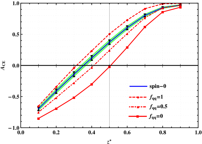
Figure 1: $A_{CE}$ as a function of $z^{*}$ for spin-0 (solid, blue, with error bars) and spin-2 hypotheses at different $f_{qq}$ (red, marked by squares and triangles) from the process (1) at ATLAS with $\sqrt{s}=$8 TeV, ${\cal L}_{\rm int}=20.7~{}\text{fb}^{-1}$. The vertical bars and corresponding green band represent 1$\sigma$ statistical uncertainties on $A_{CE}$ [26, 4], based on the observed number of events discussed in the text.

In Fig. 1 we show $A_{CE}$ as a function of $z^{*}$ for spin-0 and spin-2 for different fractions of the sub-processes ($f_{qq}$ = 0, 0.5 and 1) obtained from the distributions depicted in Fig. 5 of Ref. [4]. The center-edge asymmetry and the corresponding statistical uncertainties attached to the line of the spin-0 case shown in Fig. 1 were obtained following the “sWeight” technique developed in [26] that allows to perform excellent signal versus background separation. One should notice that $A_{CE}$ and its statistical uncertainty depicted in Fig. 1 for the spin-0 and spin-2 cases at $z^{*}=0.5$ (and with $f_{qq}=0$ for spin 2) are quite consistent with those derived in Ref. [26] (see Table 1). The figure indicates that the maximal differentiation of the observable between the different spin hypotheses occurs at $z^{*}\approx 0.4-0.6$. It should be noted that for $f_{qq}$ around 0.75, the $A_{\text{CE}}$ observable becomes useless. Typical models, however, like the Randall–Sundrum model [43], favor much lower values of $f_{qq}$, where the discriminination is substantial.

One should note that systematic uncertainties affecting the signal yield as a multiplicative factor cancel in the asymmetry $A_{CE}$. This holds for systematics on luminosity, $z$-independent selection efficiencies, theoretical errors from renormalization and factorization scale uncertainties etc. But some types of errors on an asymmetry measure (e.g. parton distribution function uncertainties, PDFs) do not cancel. A systematic error of about 3% comes from PDFs, which does not cancel in the $A_{CE}$ [26], was taken into account in the numerical analysis.

The $A_{CE}$ asymmetry obeys a Gaussian distribution with mean $\bar{A}_{CE}$ and standard deviation $\bar{\sigma}_{A_{CE}}$, which can be written as

$$\bar{\sigma}_{A_{CE}}=\sqrt{(1-{\bar{A}_{CE}}^{2})/N}.$$ (11)

To evaluate the confidence level at which the spin-2 hypothesis can be excluded we start from the assumption that spin-0 favors the experimental data as there is strong motivation for prioritizing the spin-0 hypothesis. In Fig. 1, the vertical bars attached to the solid (spin-0) line represent, again as an example, the 1$\sigma$ statistical uncertainty on $A_{CE}$ corresponding to the Higgs boson signal events. Comparison of the $A_{CE}$ difference between the spin-0 and spin-2 curves with the statistical uncertainties allows to make a simple approximate evaluation of the separation significance of the two spin hypotheses. In this analysis we adopt the assumption that the spin-2 resonance has the same mass and width as the Higgs boson, and the cross section for the production and decay of a tensor resonance is normalized by the SM Higgs rates. For example, for $f_{qq}=0$ and $z^{*}=0.5$ one obtains a separation significance of 6 to $8\sigma$.

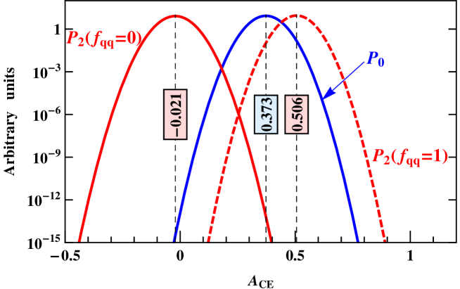
Figure 2: Probability density functions of the signal center-edge asymmetry $A_{CE}$ for spin-0 and spin-2 distributions. The $A_{CE}$ values at which the probabilities are maximized, are given in the boxes.

In Fig. 2 we show the probability density functions (pdf) for the hypotheses considered above. From the integration of the probability density functions shown in that figure one can calculate $p$-values for rejection of a hypothesis with tensor resonance. Then, one should convert the obtained $p$-value to the number of standard deviations ($\sigma$’s) as [26, 44]

$$Z(\sigma)=\Phi^{-1}(1-p)=\frac{|{\bar{A}_{0}}-{\bar{A}_{2}}|}{{\bar{\sigma}_{0}}},$$ (12)

where we denote $A_{0}=A_{CE}^{\rm spin-0}$ and $A_{2}=A_{CE}^{\rm spin-2}$, the inverse of the cumulative distribution function of the standard normal, $\Phi^{-1}(1-p)$, calculated at $1-p$, gives the standard confidence level $Z(\sigma)$ of the test in units of the standard deviation of the Gaussian distribution [44]. Furthermore, $\bar{\sigma}_{0}$ here refers to $\bar{\sigma}_{A_{CE}}$ defined above, evaluated for the spin-zero case.

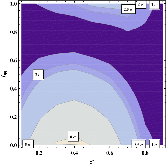
Figure 3: The significance $Z(\sigma)$ for spin-0 vs spin-2 hypotheses in the plane of ($z^{*}$, $f_{qq}$), based on $A_{CE}$ determined from ATLAS simulations for the process (1) at the LHC with $\sqrt{s}=$8 TeV and ${\cal L}_{\rm int}=20.7~{}\text{fb}^{-1}$ [4].

The center-edge asymmetry here depends on two parameters, namely the kinematical parameter $z^{*}$ and the fraction $f_{qq}$ of the $q\bar{q}$ production of the spin-2 particle. In Fig. 3 we show a contour plot in the ($z^{*}$, $f_{qq}$) plane for the separation significance $Z(\sigma)$ defined in Eq. (12) and translated into $n$ standard deviations attached to the curves, for spin-0 vs spin-2 hypotheses. Fig. 3 shows that one can optimize the kinematical parameter $z^{*}$ in order to obtain the largest separation significance. In fact, the most suitable $z^{*}$ is in the range $z^{*}=0.4-0.6$. Such optimization can be applied for the spin separation analysis within the whole range of values for the fraction $f_{qq}$.

Also, Fig. 3 shows the area (dark blue) with the smallest separation between the spin-0 and spin-2 signals which occurs for example, for $f_{qq}\approx 0.7$. In this area of smaller separation power, the method does not allow the exclusion of the spin-2 hypothesis when the Higgs-like boson is produced partially by $q\bar{q}$ annihilation. The reason is that with this admixture, the sum of the spin-2 $A_{CE}$ pdf’s associated to gluon fusion and quark-antiquark production is very similar to that of spin-0.

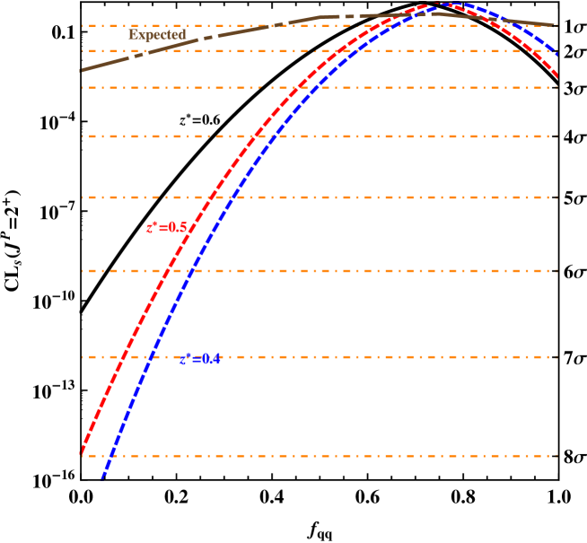
Figure 4: The confidence level, ${\rm CL_{s}}(J^{P}=2^{+})$, of the $J^{P}=2^{+}$ hypothesis as a function of the fraction $f_{qq}$ for spin-2 particle production, obtained from the center-edge asymmetry measure at different $z^{*}=$ 0.4, 0.5 and 0.6 in the $H\to\gamma\gamma$ channel at the LHC with $\sqrt{s}=8$ TeV and luminosity 20.7 ${\rm fb}^{-1}$. On the right vertical axis, the corresponding number of Gaussian standard deviations is given. The dash-dotted line represents the expected confidence level from the ATLAS analysis summarized in Table 4 of Ref. [4].

There is an alternative approach to quantify the separation power by using the CLs prescription [45]. The exclusion of the alternative spin-2 hypothesis in favor of the SM spin-0 hypothesis is evaluated in terms of the corresponding ${\rm CLs}(J^{P}=2^{+})$, defined as

$${\rm CLs}(J^{P}=2^{+})=\frac{p(J^{P}=2^{+})}{1-p(J^{P}=0^{+})},$$ (13)

where $p(J^{P}=2^{+})$ is the $p$-value for spin-2 and $p(J^{P}=0^{+})$ is the $p$-value for spin-0, respectively. Spin-2 exclusion limits as functions of $f_{qq}$ at three values of $z^{*}=$0.4, 0.5 and 0.6 computed using the CLs prescription are shown in Fig. 4.

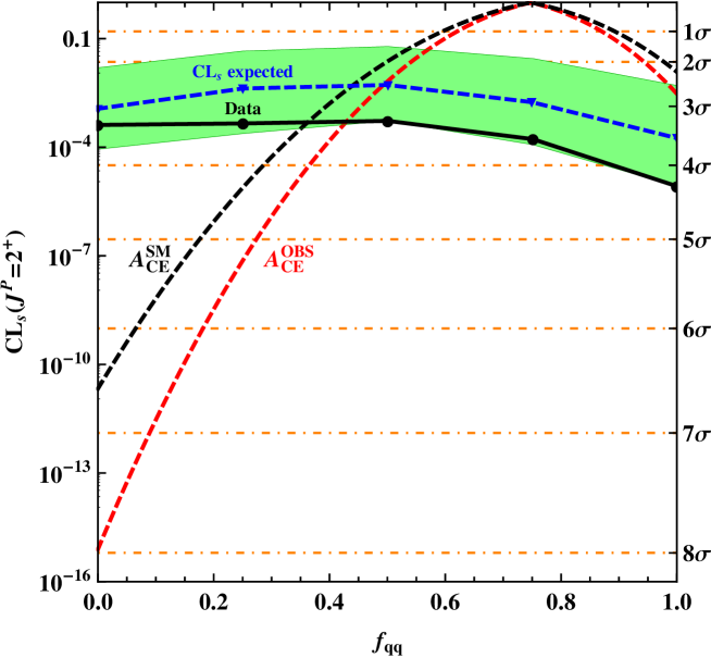
Figure 5: Comparison of the expected and observed confidence levels, ${\rm CL_{s}}(J^{P}=2^{+})$, of the $J^{P}=2^{+}$ hypothesis as functions of the fraction $f_{qq}$ for spin-2 particle production. Expected (blue triangles/dashed line) and observed (black circles/solid line) confidence levels are based on the experimental data and obtained from the combination of the angular distributions of the three channels $H\to\gamma\gamma$, $H\to ZZ^{*}$ and $H\to WW^{*}$ at $\sqrt{s}=7$ and 8 TeV with ATLAS [3]. The green band represents the 68% expected exclusion range for a signal with assumed $J^{P}=0^{+}$. On the right vertical axis, the corresponding number of Gaussian standard deviations is given. The center-edge asymmetry measure, applied to the $H\to\gamma\gamma$ channel at $z^{*}=0.5$, yields the expected ($A_{\rm CE}^{\rm SM}$) and observed ($A_{\rm CE}^{\rm OBS}$) confidence levels shown as dashed black and red curves.

It is instructive to compare the confidence level, obtained in the present analysis with those available from the ATLAS study of the three channels $H\to\gamma\gamma$, $H\to ZZ^{*}$ and $H\to WW^{*}$ at $\sqrt{s}=8$ TeV and luminosity 20.7 ${\rm fb}^{-1}$ [3]. Fig. 5 shows that $A_{CE}$ measurements are able to substantially increase the observed confidence level, in particular in the range of parameter space where $0<f_{qq}<0.4$. In other words, in this range of $f_{qq}$, $A_{CE}$ provides quite competitive information on the spin of the Higgs-like boson with respect to that derived from the commonly used analysis of angular distributions.

The result obtained from the $A_{\text{CE}}$ observable obviously depends on the number of events in this channel. Since the signal strength observed by ATLAS has recently been somewhat reduced, due in part to an improved photon energy calibration [7] and diphoton mass resolution, we show in Fig. 5 two curves: one corresponding to the observed angular distribution [3, 4] (670 events, labeled $A_{\text{CE}}^{\text{OBS}}$) and one corresponding to the SM expectation (390 events, labeled $A_{\text{CE}}^{\text{SM}}$).

3 Concluding remarks

We have studied the possibility to determine the spin of the Higgs-like boson with the center-edge asymmetry in the $H\to\gamma\gamma$ channel at ATLAS with 8 TeV and integrated luminosity of $20.7~{}\text{fb}^{-1}$. In the present analysis we compared the spin-0 hypothesis of the Higgs-like boson with that of a graviton-like, spin-2, particle with minimal couplings, taking into account the possibility that the tensor particle might be produced via quark-antiquark annihilation or gluon fusion. We obtained the discrimination power as a function of two parameters, the dynamical one $f_{qq}$ that determines the fraction of the $q\bar{q}$ mode in the resonance production, and the kinematical one $z^{*}$ that defines the center-edge asymmetry.

Optimization of the separation significance on the kinematical parameter $z^{*}$ at different $f_{qq}$ allows to find the region in the parameter plane where the center-edge asymmetry could provide quite competitive information on the spin of the Higgs-like boson with respect to that which is derived from the more common angular-distribution analysis. We found that $A_{\text{CE}}$ provides discrimination between the scalar and tensor hypotheses with ${\rm CL_{s}}<10^{-6}$ at $f_{qq}=0$ and $z^{*}\approx 0.4$, a value that substantially exceeds the ATLAS expectations. For increasing values of $f_{qq}$, the expected separation between spin-0 and spin-2 hypotheses is reduced, reaching a minimum at $f_{qq}\approx 0.75$ where separation is impossible. At higher energies, however, the gluon-gluon contribution would tend to increase, thus strengthening the usefulness of $A_{\text{CE}}$.

References

- [1] G. Aad et al. [ATLAS Collaboration], Phys. Lett. B 716, 1 (2012) [arXiv:1207.7214 [hep-ex]].
- [2] S. Chatrchyan et al. [CMS Collaboration], Phys. Lett. B 716, 30 (2012) [arXiv:1207.7235 [hep-ex]].
- [3] G. Aad et al. [ATLAS Collaboration], Phys. Lett. B 726, 120 (2013) [arXiv:1307.1432 [hep-ex]].
- [4] [ATLAS Collaboration], ATLAS-CONF-2013-029.
- [5] S. Chatrchyan et al. [CMS Collaboration], Phys. Rev. D 89, 092007 (2014) [arXiv:1312.5353 [hep-ex]].
- [6] V. Khachatryan et al. [CMS Collaboration], Eur. Phys. J. C 74, 3076 (2014) [arXiv:1407.0558 [hep-ex]].
- [7] G. Aad et al. [ATLAS Collaboration], Phys. Rev. D 90, 112015 (2014) [arXiv:1408.7084 [hep-ex]].
- [8] V. Khachatryan et al. [CMS Collaboration], arXiv:1411.3441 [hep-ex].
- [9] L. D. Landau, Dokl. Akad. Nauk Ser. Fiz. 60, 207 (1948).
- [10] C. N. Yang, Phys. Rev. 77, 242 (1950).
- [11] [ATLAS Collaboration], ATLAS-CONF-2013-040.
- [12] S. Y. Choi, D. J. Miller, M. M. Muhlleitner and P. M. Zerwas, Phys. Lett. B 553, 61 (2003) [hep-ph/0210077].
- [13] Y. Gao, A. V. Gritsan, Z. Guo, K. Melnikov, M. Schulze and N. V. Tran, Phys. Rev. D 81, 075022 (2010) [arXiv:1001.3396 [hep-ph]].
- [14] A. De Rujula, J. Lykken, M. Pierini, C. Rogan and M. Spiropulu, Phys. Rev. D 82, 013003 (2010) [arXiv:1001.5300 [hep-ph]].
- [15] C. Englert, C. Hackstein and M. Spannowsky, Phys. Rev. D 82, 114024 (2010) [arXiv:1010.0676 [hep-ph]].
- [16] S. Bolognesi, Y. Gao, A. V. Gritsan, K. Melnikov, M. Schulze, N. V. Tran and A. Whitbeck, Phys. Rev. D 86, 095031 (2012) [arXiv:1208.4018 [hep-ph]].
- [17] S. Y. Choi, M. M. Muhlleitner and P. M. Zerwas, Phys. Lett. B 718, 1031 (2013) [arXiv:1209.5268 [hep-ph]].
- [18] C. Englert, D. Goncalves-Netto, K. Mawatari and T. Plehn, JHEP 1301, 148 (2013) [arXiv:1212.0843 [hep-ph]].
- [19] S. Banerjee, J. Kalinowski, W. Kotlarski, T. Przedzinski and Z. Was, Eur. Phys. J. C 73, 2313 (2013) [arXiv:1212.2873 [hep-ph]].
- [20] A. Menon, T. Modak, D. Sahoo, R. Sinha and H. Y. Cheng, Phys. Rev. D 89, 095021 (2014) [arXiv:1301.5404 [hep-ph]].
- [21] D. Boer, W. J. den Dunnen, C. Pisano and M. Schlegel, Phys. Rev. Lett. 111, no. 3, 032002 (2013) [arXiv:1304.2654 [hep-ph]].
- [22] J. Frank, M. Rauch and D. Zeppenfeld, Eur. Phys. J. C 74, 2918 (2014) [arXiv:1305.1883 [hep-ph]].
- [23] C. Englert, D. Goncalves, G. Nail and M. Spannowsky, Phys. Rev. D 88, 013016 (2013) [arXiv:1304.0033 [hep-ph]].
- [24] R. Boughezal, T. J. LeCompte and F. Petriello, arXiv:1208.4311 [hep-ph].
- [25] J. Ellis, D. S. Hwang, V. Sanz and T. You, JHEP 1211, 134 (2012) [arXiv:1208.6002 [hep-ph]].
- [26] A. Alves, Phys. Rev. D 86, 113010 (2012) [arXiv:1209.1037 [hep-ph]].
- [27] C. Q. Geng, D. Huang, Y. Tang and Y. L. Wu, Phys. Lett. B 719, 164 (2013) [arXiv:1210.5103 [hep-ph]].
- [28] J. Ellis, R. Fok, D. S. Hwang, V. Sanz and T. You, Eur. Phys. J. C 73, 2488 (2013) [arXiv:1210.5229 [hep-ph]].
- [29] A. Djouadi, R. M. Godbole, B. Mellado and K. Mohan, Phys. Lett. B 723, 307 (2013) [arXiv:1301.4965 [hep-ph]].
- [30] P. Osland, A. A. Pankov and N. Paver, Phys. Rev. D 68, 015007 (2003) [hep-ph/0304123].
- [31] E. W. Dvergsnes, P. Osland, A. A. Pankov and N. Paver, Phys. Rev. D 69, 115001 (2004) [hep-ph/0401199].
- [32] E. W. Dvergsnes, P. Osland, A. A. Pankov and N. Paver, Int. J. Mod. Phys. A 20, 2232 (2005) [hep-ph/0410402].
- [33] P. Osland, A. A. Pankov, N. Paver and A. V. Tsytrinov, Phys. Rev. D 78, 035008 (2008) [arXiv:0805.2734 [hep-ph]].
- [34] P. Osland, A. A. Pankov, A. V. Tsytrinov and N. Paver, Phys. Rev. D 79, 115021 (2009) [arXiv:0904.4857 [hep-ph]].
- [35] P. Osland, A. A. Pankov, N. Paver and A. V. Tsytrinov, Phys. Rev. D 82, 115017 (2010) [arXiv:1008.1389 [hep-ph]].
- [36] M. C. Kumar, P. Mathews, A. A. Pankov, N. Paver, V. Ravindran and A. V. Tsytrinov, Phys. Rev. D 84, 115008 (2011) [arXiv:1108.3764 [hep-ph]].
- [37] J. C. Collins and D. E. Soper, Phys. Rev. D 16, 2219 (1977).
- [38] C. A. Nelson, Phys. Rev. D 37, 1220 (1988).
- [39] A. Skjold and P. Osland, Phys. Lett. B 311, 261 (1993) [hep-ph/9303294].
- [40] R. M. Godbole, D. J. Miller and M. M. Muhlleitner, JHEP 0712, 031 (2007) [arXiv:0708.0458 [hep-ph]].
- [41] K. m. Cheung, Phys. Rev. D 61, 015005 (2000) [hep-ph/9904266].
- [42] O. J. P. Eboli, T. Han, M. B. Magro and P. G. Mercadante, Phys. Rev. D 61, 094007 (2000) [hep-ph/9908358].
- [43] L. Randall and R. Sundrum, Phys. Rev. Lett. 83, 3370 (1999) [hep-ph/9905221].
- [44] J. Beringer et al. [Particle Data Group Collaboration], Phys. Rev. D 86, 010001 (2012).
- [45] A. L. Read, J. Phys. G 28, 2693 (2002).