Wave Propagation in 1-D Spiral geometry

Abstract

In this article, we investigate the wave equation in spiral geometry and study the modes of vibrations of a one-dimensional (1-D) string in spiral shape. Here we show that the problem of wave propagation along a spiral can be reduced to Bessel differential equation and hence, very closely related to the problem of radial waves of two-dimensional (2-D) vibrating membrane in circular geometry.

Our goal is to study the modes of a string bent along a spiral. At the first glance, the problem appears to be only of academic interest. However, it should be noted that the spiral geometries are common in nature, specially those related to wave propagations. The most popular of spiral geometry, namely logarithmic spiral manifests itself frequently in the nature in various forms. For example, simple conch to arms of the majorities of galaxies are in spiral shape. Also, one of the most efficient waveguides in nature, the inner ear of mammals, is also a spiral! It has been shown that, the spiral shape of Basilar membrane plays an important role in hearing [1]. Here, we study the normal modes of vibration in this geometry and hope to understand its significance.

Though there is vast amount of literature on the wave equation in standard geometries [2, 3, 4], there has been little work in the spiral coordinate system, especially at the undergraduate level. In our approach, we first do a coordinate transform to reduce the wave equation to a Bessel differential equation. This makes the problem similar to that of radial part of wave equation in circular geometry or radial part of circular vibrating membrane. The solutions are expressed in terms of the Bessel and Neumann functions and in general, the modes are not integral multiples of fundamental mode. We investigate the solutions satisfying some of the standard boundary conditions.

1 Spiral geometry and the wave equation

In this section, we discuss the geometry of logarithmic spiral. We would like to have spiral connecting between $r_{i}$ to $r_{o}$ after taking $n$ turns as shown in the Fig. (1.1). The equation for logarithmic spiral is given by:

$$r=r_{i}e^{\mu\theta}\,,$$ (1.1)

where, $\mu$ describes how fast the spiral is accelerating outwards. We would like to parameterize the spiral only in terms of $r_{i}$, $r_{o}$ and $n$. Expressing $\mu$ in terms of these parameters, we have:

$$\mu=\frac{1}{2\pi n}\log\left(\frac{r_{o}}{r_{i}}\right)\,.$$ (1.2)

We see that, Larger number of turns, spiral slowly progresses outwards. The length of the spiral is given by $s=\intop_{0}^{2n\pi}ds$, where $ds=\sqrt{r^{2}+\left(\frac{dr}{d\theta}\right)^{2}}\>d\theta$. For logarithmic spiral we get:

$$s=\sqrt{\left(1+\frac{1}{\mu^{2}}\right)}\left(r_{o}-r_{i}\right)\,.$$ (1.3)

Considering the relation between $\mu$ and $n$ as given in Eq. (1.2), we see that the length is proportional to the number of turns $n$. Here, we could like to note that $n$ need not be integer, it gives the measure of angle in terms of $2\pi$ radians.

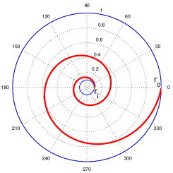
Figure 1.1: Spiral starts at inner radius $r_{i}=0.1$ and reaches location $r_{o}=1$ after taking two turns.

Next, we investigate the wave equation in the spiral geometry. We start with the scalar wave equation in the 2-D polar coordinates $\left(r,\,\theta\right)$, given by:

$$\frac{1}{r}\frac{\partial}{\partial r}\left(r\frac{\partial\psi}{\partial r}\right)+\frac{1}{r^{2}}\frac{\partial^{2}\psi}{\partial\theta^{2}}-\frac{1}{c^{2}}\frac{\partial^{2}\psi}{\partial t^{2}}=0\,.$$ (1.4)

We constrain this wave equation along a logarithmic spiral. Using Eq. (1.1), we directly substituting for $\frac{\partial}{\partial\theta}$ and $\frac{\partial^{2}}{\partial\theta^{2}}$ as:

$$\frac{\partial^{2}\psi}{\partial\theta^{2}}=\mu^{2}r^{2}\frac{\partial^{2}\psi}{\partial r^{2}}+\mu^{2}r\frac{\partial\psi}{\partial r}\,.$$ (1.5)

After substitution and simplification, we obtain:

$$r^{2}\frac{d^{2}}{dr^{2}}\psi\left(r\right)+r\frac{d}{dr}\psi\left(r\right)+k^{2}r^{2}\psi\left(r\right)=0\,,$$ (1.6)

where,

$$k^{2}=\frac{\omega^{2}}{c^{2}\left(1+\mu^{2}\right)}\,.$$ (1.7)

Here, for simplicity, we replace $\frac{\partial\psi}{\partial r}$ by $\frac{d\psi}{dr}$. From Eq. (1.7), we see that the spatial frequencies are scaled a factor of $\left(1+\mu^{2}\right)^{-\frac{1}{2}}$. The relation between $k$ and $\omega$, the dispersion relation, clearly depends on the geometry of the spiral. Plot of $\frac{c^{2}k^{2}}{\omega^{2}}$ as function of number of turns $n$ is shown in Fig. (1.2). When the number of turn becomes large, the relation reduce to that in of a straight string. However, when $n$ is small, we see the scaling of the spatial frequencies. In the case of linear string, the dispersion relation leads to the conventional relation $c=f\lambda$, where $\lambda$ is wavelength, $f=\omega/2\pi$ is frequency and $c$ is the speed of the wave. In spiral geometry, this relation needs to be corrected by a geometric factor as given by Eq. (1.7). Overall, for a given frequency, wavelength is longer by a factor of $\sqrt{1+\mu^{2}}$, compared to a linear-string.

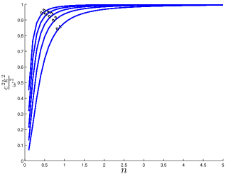
Figure 1.2: Plot of dispersion relation as function of number of turns, ’$n$’.

The wave equation on the spiral, given by Eq. (1.6), is the well known Bessel differential equation. The general solutions are given in terms of Bessel and Neumann functions as:

$$\psi=A_{1}J_{0}\left(kr\right)+B_{1}N_{0}\left(kr\right)\,,$$ (1.8)

where $J_{0}$ and $N_{0}$, are Bessel and Neumann function of order zero respectively. However, we need to investigate the solutions with physically important boundary conditions which may constrain solutions and frequencies. In the next sub-section we study some of the boundary conditions. One important point to notice here is the similarity in the solution along a spiral and that in the radial wave equation in the plane-polar geometry. In both we get the Bessel differential equation.

2 Spiral string fixed at both ends

In this section, we extend the classic linear vibrating string problem (see [2] for extensive details) with both end fixed to spiral geometry. Let the inner and outer ends of a finite spiral string are fixed at $r=r_{i}$ and $r=r_{o}$, respectively. Explicitly, the boundary conditions are given by $\psi\left(r=r_{i},\,t\right)=\psi\left(r=r_{o},\,t\right)=0$, without loss of generality, the solution can be written as:

$$\psi=\sum_{n=1}A_{n}\left[\cos\delta\>J_{0}\left(\kappa_{n}r\right)+\sin\delta\>N_{0}\left(\kappa_{n}r\right)\right]\cos\omega_{n}t\,.$$ (2.1)

Here, $\delta$ is chosen such that, the boundary condition at $r=r_{o}$ is satisfied, resulting in the condition:

$$\tan\delta=-\frac{J_{0}\left(\kappa_{n}r_{o}\right)}{N_{0}\left(\kappa_{n}r_{o}\right)}\,.$$ (2.2)

However, all values of $\kappa_{n}$ will not satisfy the boundary condition at $r_{i}$ and the allowed values of $\kappa_{n}$ can be determined from the equation:

$$\cos\delta\>J_{0}\left(\kappa_{n}r_{i}\right)+\sin\delta\>N_{0}\left(\kappa_{n}r_{i}\right)=0\,.$$ (2.3)

Numerical solutions for $\kappa_{n}$ for $n=1$ to $5$ is obtained for few values of $r_{i}$, with fixed value of $r_{o}=1$ and are tabulated in Table 1. Corresponding frequencies, $\omega_{n}$ can be obtained from the relation given in Eq. (1.7). The eigenfrequencies play important role because they correspond to the resonance condition, giving the modes at which string vibrates.

$r_{i}$	$r_{o}$	$k_{1}$	$k_{2}$	$k_{3}$	$k_{4}$	$k_{5}$
$0.1$	$1.0$	3.313	6.857	10.37	13.88	17.38
$0.2$	$1.0$	3.815	7.785	11.73	15.67	19.60
$0.3$	$1.0$	4.412	8.932	13.43	17.92	22.42
$0.4$	$1.0$	5.183	10.44	15.68	20.92	26.16
$0.5$	$1.0$	6.246	12.54	18.83	25.12	31.40

Table 1: Roots of Eq. (2.3) for various values of $r_{i}$ and $r_{o}$.

2.1 Finite Spiral string with vibrating ring

Here, we consider the boundary condition such that, outer end of a string is rigidly fixed at $r=r_{o}$, while the inner end at $r=r_{i}$ is attached to a oscillating ring with frequency $\Omega$. The corresponding boundary conditions can be written as $\psi\left(r=r_{i},\,t\right)=F\cos\Omega t$, with oscillating circle and $\psi\left(r=r_{o},\,t\right)=0$. Any Solution, can now be written terms of linear combination of Bessel and Neumann function as:

$$\psi=A\left[\cos\delta\>J_{0}\left(\kappa r\right)+\sin\delta\>N_{0}\left(\kappa r\right)\right]\cos\Omega t\,.$$ (2.4)

The constants $A$ and $\delta$ need to be determined from the boundary conditions. As in the previous case, from the boundary condition at $r_{o}$, i.e $\psi\left(r=r_{o},\,t\right)=0$, we get:

$$\tan\delta=-\frac{J_{0}\left(\kappa r_{o}\right)}{N_{0}\left(\kappa r_{o}\right)}\,.$$ (2.5)

In addition, from the boundary condition at $r=r_{i}$, we get:

$$A=\frac{F}{\left[\cos\delta\>J_{0}\left(\kappa r_{i}\right)+\sin\delta\>N_{0}\left(\kappa r_{i}\right)\right]}\,.$$ (2.6)

As expected, at resonance, we will not be able to determine the constant $A$, the solution becomes undefined.

3 Conclusion

Spiral geometry offers interesting solutions to the wave equation with various physically important boundary conditions. Further interesting solutions maybe obtained by using different densities along the string, as is known for the case of Indian drums [6, 7]. The connection between 2-D circular and 1-D spiral is important as wave equation in circular geometry is well understood and one can apply some of the implications immediately to the spiral geometry. Similarities between circular drum head and spiral string is indeed a useful result since the entire membrane can be replaced by a 1-D spring giving the same vibration modes. This can come handy since the material required to create a membrane can be done with by using the spiral.

The more general case may be dealt by transforming from Cartesian coordinates to a coordinate system where constant curves are spirals [5]. The solutions of 2-D wave equation in such a system can also be given in terms of Bessel functions, which will be discussed else where. Since analytic solutions are available, otherwise complete numerical analysis can be avoided for the applications such as vibration isolator with spiral/helical suspension. One the important application under consideration is the wave propagation in the basilar membrane of mammals. It has already been shown that, the spiral geometry of inner ears of mammals has important implications [1], this may be further extended using results from spiral coordinates.

References

- [1] D. Manoussaki, E.K. Dimitriadis, and R.S. Chadwick, Phys. Rev. Lett. 96, 088701 (2006).
- [2] Coulson, Charles Alfred, and Alan Jeffrey. Waves: A mathematical approach to the common types of wave motion. London: Longman (1977).
- [3] Arfken, George B., and Hans J. Weber. Mathematical Methods For Physicists International Student Edition. Academic press (2005).
- [4] Morse, Philip McCord, and Hermann Feshbach. Methods of theoretical physics. (1953).
- [5] LMBC Campos and PJS Gil, Journal of Fluid Mechanics, 301,153-173 (1995).
- [6] Hagues and Piette, Modelling the Indian drum (2010).
- [7] Raman, C. V. Proceedings of the Indian Academy of Sciences Sec. A, 1, No. 3. Springer India (1934).