Nonparametric model checks of single-index assumptions

Abstract

Semiparametric single-index assumptions are convenient and widely used dimension reduction approaches that represent a compromise between the parametric and fully nonparametric models for regressions or conditional laws. In a mean regression setup, the SIM assumption means that the conditional expectation of the response given the vector of covariates is the same as the conditional expectation of the response given a scalar projection of the covariate vector. In a conditional distribution modeling, under the SIM assumption the conditional law of a response given the covariate vector coincides with the conditional law given a linear combination of the covariates. Several estimation techniques for single-index models are available and commonly used in applications. However, the problem of testing the goodness-of-fit seems less explored and the existing proposals still have some major drawbacks. In this paper, a novel kernel-based approach for testing SIM assumptions is introduced. The covariate vector needs not have a density and only the index estimated under the SIM assumption is used in kernel smoothing. Hence the effect of high-dimensional covariates is mitigated while asymptotic normality of the test statistic is obtained. Irrespective of the fixed dimension of the covariate vector, the new test detects local alternatives approaching the null hypothesis slower than $n^{-1/2}h^{-1/4},$ where $h$ is the bandwidth used to build the test statistic and $n$ is the sample size. A wild bootstrap procedure is proposed for finite sample corrections of the asymptotic critical values. The small sample performances of our test compared to existing procedures are illustrated through simulations.

Keywords. Single-index regression, conditional law, lack-of-fit test, kernel smoothing, $U-$statistics

I Introduction

Semiparametric single index models (SIM) are widely used tools for statistical modeling. The paradigm of such models is based on the assumption that the information contained in a vector of conditioning random variables is equivalent, in some sense, to the information contained in some index, that is usually a linear combination of the vector components. This assumption underlies most of the statistical parametric models including covariates, but allows for more general semiparametric modeling. The most common semiparametric SIM are those for the mean regression. See Powell et al. (1989), Ichimura (1993), Härdle et al. (1993), see also Horowitz (2009) for a recent review. In such models, the index and the conditional mean given the index are unknown. SIM for quantile regression were considered recently, see Kong and Xia (2012). A more restrictive, but still of significant interest, class of models is obtained by imposing the single-index paradigm to the conditional distribution of response variable given a vector of covariates. In these cases the index and the conditional law of the response given the index are unknown. The famous Cox proportional hazard model, see Cox (1972), is a particular case of SIM for conditional laws. See Delecroix et al. (2003), Hall and Yao (2005), Chiang and Huang (2012) for more general situations.

The large amount of interest for SIM could be explained by the fact that the single-index assumption is very often the first intermediate step from a parametric framework towards a fully nonparametric paradigm. Then an important question is whether this dimension reduction compromise is good enough to capture the relevant information contained in the covariate vector. A possible way to answer is to build a statistical test of the single-index assumption against general alternatives. Several tests of the goodness-of-fit of single-index mean regression models have proposed in the literature. See Fan and Li (1996), Xia et al. (2004), Stute and Zhu (2005), Chen and Van Keilegom (2009), Escanciano and Song (2010) and the references therein. The problem of testing SIM models for conditional distribution in full generality seems open.

In this paper we propose a new and quite simple kernel smoothing-based approach for testing single-index assumptions. We focus on mean regression and conditional law models. The approach is inspired by the remark that, up to some error in covariates, the single-index assumption check could be interpreted as a test of significance in nonparametric regression. Next, the single-index assumption could be conveniently reformulated as an equivalent unconditional moment condition. Finally, a kernel based test statistic could be used to test the unconditional moment condition. The smoothing based goodness-of-fit test approach allows to make the error in covariates negligible and thus to obtain a pivotal asymptotic law under the null hypothesis. The covariate vector needs not have a density, discrete covariables are allowed. Only the index estimated under the SIM assumption is used in kernel smoothing and this fact mitigates the effect of high-dimensional covariates. Meanwhile the asymptotical critical values are given by the quantiles of the normal law. Irrespective of the fixed dimension of the covariate vector, the new test detects local alternatives approaching the null hypothesis slower than $n^{-1/2}h^{-1/4},$ where $h$ is the bandwidth used to build the test statistic and $n$ is the sample size.

The paper is organized as follows. In Section II, we recall general considerations on single-index models. In Section III, we present a general approach of testing nonparametric significance and in Section IV we apply it to single-index hypotheses for mean regression as well as for conditional law. In Section V we introduce a wild bootstrap procedure to correct the asymptotic critical values with small samples and illustrate the performance of our test by an empirical study. Technical results and proofs are relegated to the appendix.

II Single-index models

Let $Y\in\mathbb{R}^{d},$ $d\geq 1,$ denote the random response vector and let $X\in\mathbb{R}^{p},$ $p\geq 1,$ be the random column vector of covariates. The data consists of independent copies of $(Y^{\prime},X^{\prime})^{\prime}.$ For mean regression the single-index assumption means that there exists a column parameter vector $\beta_{0}\in\mathbb{R}^{p}$ such that

$$\mathbb{E}[Y\mid X]=\mathbb{E}[Y\mid X^{\prime}\beta_{0}].$$ (II.1)

Only the direction given by $\beta_{0}$ is identified, so that an additional identification condition accompanies the model assumption, as for instance $\|\beta_{0}\|=1$ and an arbitrary component is set positive, or an arbitrary component is set to 1. The scalar product $X^{\prime}\beta_{0}$ is the so-called index. The direction $\beta_{0}$ and the nonparametric univariate regression $\mathbb{E}[Y\mid X^{\prime}\beta_{0}]$ have to be estimated. See Hristache et al. (2001), Delecroix et al. (2006), Horowitz (2009), Xia et al. (2011) and the references therein for a panorama of the existing estimation procedures.

When applying the single-index paradigm to conditional laws of $Y$ given $X,$ one supposes

$$Y\perp X\mid X^{\prime}\beta_{0}.$$ (II.2)

In this case the direction defined by $\beta_{0}$ and the conditional law of the response $Y$ given the index $X^{\prime}\beta_{0}$ have to be estimated. See Delecroix et al. (2003), Hall and Yao (2005) and Chiang and Huang (2012) for the available estimation approaches.

There are several model check approaches for SIM for mean regressions. Xia et al. (2004) use an empirical process-based statistic related to that of Stute et al. (1998). Fan and Li (1996) use a kernel smoothing-based quadratic form to a wide range of situations, including single-index. Our test statistics are somehow close to that of Fan and Li (1996). Chen and Van Keilegom (2009) use an empirical likelihood test for multi-dimensional $Y$ in a parametric or semiparametric modeling, the single-index mean regression is presented as a particular case but without getting into the details.

In this paper we propose an alternative model check approach that is able to detect any departure from the single-index assumption, both for mean regressions and conditional law models. It is inspired by a general approach for testing nonparametric significance that is presented in the following section.

III A general approach for testing nonparametric significance

Let $(\mathcal{H},\langle\cdot,\cdot\rangle_{\mathcal{H}})$ be a Hilbert space. The examples we have in mind corresponds to $\mathcal{H}=\mathbb{R}^{d},$ for some $d\geq 1,$ or $\mathcal{H}=L^{2}[0,1].$ Consider $U\in\mathcal{H}$, $Z\in\mathbb{R}^{q}$ et $W\in\mathbb{R}^{r}$ and let $(U_{i},Z_{i},W_{i})$, $1\leq i\leq n$ denote an independent sample of $U$, $Z$ and $W$. Consider the problem of testing the equality

$$\mathbb{E}[U\mid Z,W]=0\qquad\text{p.s.}$$ (III.3)

against the nonparametric alternative $\mathbb{P}(\mathbb{E}[U\mid Z,W]=0)<1.$ Several testing procedures against nonparametric alternatives, including the single-index assumptions check, lead to this type of problem.

Let us introduce some notation: for any real-valued, univariate or multivariate function $l$, let $\mathcal{F}[l]$ denote the Fourier Transform of $l$. Let $K$ be a multivariate kernel $\mathbb{R}^{q}$ such that $\mathcal{F}[K]>0$ and let $\phi(s)=\exp(-\|s\|^{2}/2),$ $\forall s\in\mathbb{R}^{r}.$ The kernel $K$ could be a multiplicative kernel with univariate kernels with positive Fourier Transform. Many univariate kernels have this property: gaussian, triangle, Student, logistic, etc.

Our approach is based on the following remark; see also Lavergne et al. (2014). Let $w(\cdot)>0$ be some weight function. For any $h>0$, let

$$I(h)=\mathbb{E}\left[\langle U_{1},U_{2}\rangle_{\mathcal{H}}\;w(Z_{1})w(Z_{2})h^{-q}K((Z_{1}-Z_{2})/h)\phi(W_{1}-W_{2})\right]\\ =\mathbb{E}\left[\langle U_{1},U_{2}\rangle_{\mathcal{H}}\;w(Z_{1})w(Z_{2})\int_{\mathbb{R}^{q}}e^{2\pi iv^{\prime}(Z_{1}-Z_{2})}\mathcal{F}[K](vh)dv\int_{\mathbb{R}^{r}}e^{2\pi is^{\prime}(W_{1}-W_{2})}\mathcal{F}[\phi](s)ds\right]\\ =\int_{\mathbb{R}^{q}}\int_{\mathbb{R}^{r}}\left\|\mathbb{E}\left[\mathbb{E}[U\mid Z,W]w(Z)e^{-i\{v^{\prime}Z+s^{\prime}W\}}\right]\right\|_{\mathcal{H}}^{2}\mathcal{F}[K](vh)\mathcal{F}[\phi](s)dtds.$$ (III.4)

Since $\mathcal{F}[\phi],\mathcal{F}[K]>0,$ and $w(\cdot)>0$, the following equivalence holds true: $\forall h>0$,

$$\mathbb{E}[U\mid Z,W]=0\;\;p.s.\;\;\Leftrightarrow\;\;I(h)=0.$$

To check condition (III.3) the idea is to build a sample based approximation of $I(h),$ to suitably normalize it and to let $h$ to decrease to zero. A convenient choice of $w(\cdot)$ could avoid handling denominators close to zero.

In many situations the sample of the variable $Uw(Z)$ is not observed and has to be estimated inside the model. Then, an estimate of $I(h)$ is given by the $U-$statistic

$$I_{n}(h)=\frac{1}{n(n-1)h^{q}}\sum\limits_{1\leq i\neq j\leq n}\left\langle\widehat{U_{i}w(Z_{i})},\;\widehat{U_{j}w(Z_{j})}\right\rangle_{\mathcal{H}}K_{ij}(h)\;\phi_{ij},$$

where

$$K_{ij}(h)=K((Z_{i}-Z_{j})/h),\qquad\phi_{ij}=\exp(-\|W_{i}-W_{j}\|^{2}/2).$$

The variance of $I_{n}(h)$ could be estimated by

$$v^{2}_{n}(h)=\frac{2}{n^{2}(n-1)^{2}h^{2q}}\sum\limits_{1\leq i\neq j\leq n}\left\langle\widehat{U_{i}w(Z_{i})},\;\widehat{U_{j}w(Z_{j})}\right\rangle^{2}_{\mathcal{H}}K^{2}_{ij}(h)\;\phi^{2}_{ij}.$$

Then the test statistic is

$$T_{n}=\frac{I_{n}(h)}{v_{n}(h)}.$$

Under mild technical conditions and provided that $h$ converges to zero at a suitable rate, $T_{n}$ converges in law to a standard normal distribution provided that condition (III.3) holds true. Hence, a one-sided test with standard normal critical values could be defined; see Lavergne et al. (2014). One could also show $T_{n}$ tends to infinity in probability if $\mathbb{P}(\mathbb{E}[U\mid Z,W]=0)<1.$ Making $h$ to decrease to zero at suitable rate allows to render negligible the effect of the errors $\widehat{U_{i}w(Z_{i})}-{U_{i}w(Z_{i})}.$ On the other hand, the test detects Pitman alternative hypotheses like

$$H_{1n}:\ \mathbb{E}(U\mid Z,W)=r_{n}\delta(Z,W),\quad n\geq 1,\;$$ (III.5)

as soon as $r_{n}^{2}nh^{q/2}\rightarrow\infty$.

IV Single-index assumptions checks

In this section we extend the approach described in section (III) to test single-index assumptions like (II.1) and (II.2). In this case, with the notation from section III,

$$q=1,\;\;r=p-1,\;\;Z=Z(\beta)\;\;\text{ and }\;\;W=W(\beta)$$

where, for $\beta\in\mathcal{B}\subset\mathbb{R}^{p},$

$$Z(\beta)=X^{\prime}\beta\qquad\text{et}\qquad W(\beta)=X^{\prime}\mathbf{A}\left(\beta\right)$$

with $\mathbf{A}\left(\beta\right)$ a $p\times(p-1)$ matrix with real entries such that the $p\times p$ matrix $\left(\beta\;\mathbf{A}\left(\beta\right)\right)$ is orthogonal. The orthogonality is not necessary, invertibility suffices, but orthogonality is expected to lead to better finite sample properties for the tests.

An additional challenge will come from the fact that the sample of the covariates $Z$ and $W$ depend on estimator of the single-index direction $\beta_{0}.$ Again, the kernel smoothing and a suitable choice of $h$ allows to render this effect negligible and preserve a pivotal asymptotic law under the null hypothesis.

IV.1 Testing SIM for mean regression

To simplify the presentation, let us focus on the case of a univariate response, that is $d=1.$ At the end, it will be quite clear how the case $d>1$ could be handled. To restate the single-index condition (II.1), let $\mathcal{H}=\mathbb{R},$ $Uw(Z)=U(\beta_{0})w(Z;\beta_{0})$ where

$$U(\beta)w(Z;\beta)=\{Y-\mathbb{E}[Y\mid Z(\beta)]\}f_{\beta}(Z(\beta)).$$

Here $f_{\beta}(\cdot)$ denotes the density of $X^{\prime}\beta$ that is supposed to exist, at least for some $\beta.$ Let

$$\widehat{U_{i}w(Z_{i})}(\beta)=\frac{1}{n-1}\sum\limits_{k\neq i}(Y_{i}-Y_{k})\frac{1}{g}L_{ik}(\beta,g),$$ (IV.6)

where $L$ is a univariate kernel, $L_{ik}(\beta,g)=L((Z_{i}(\beta)-Z_{k}(\beta))/g)$ and $g$ is a bandwidth converging to zero at some suitable rate described in a following section. Let $\hat{\beta}$ be some estimator of the index direction and consider

$$I_{n}^{\{m\}}(\hat{\beta}) = \dfrac{1}{n\left(n-1\right)h}\sum_{1\leq i\neq j\leq n}\widehat{U_{i}w(Z_{i})}(\hat{\beta})\widehat{U_{j}w(Z_{j})}(\hat{\beta})K_{ij}(\hat{\beta},h)\phi(W_{i}(\hat{\beta})-W_{j}(\hat{\beta})),$$

where $K_{ij}(\hat{\beta},h)=K((Z_{i}(\hat{\beta})-Z_{j}(\hat{\beta}))/h).$ The variance of $I_{n}^{\{m\}}(\hat{\beta})$ could be estimated by

$$\hat{\omega}_{n}^{\{m\}}(\hat{\beta})^{2}=\dfrac{2}{n^{2}\left(n-1\right)^{2}h^{2}}\sum_{1\leq i\neq j\leq n}\!\!\left[\widehat{U_{i}w(Z_{i})}(\hat{\beta})\widehat{U_{j}w(Z_{j})}(\hat{\beta})\right]^{2}K_{ij}^{2}(\hat{\beta},h)\phi^{2}(W_{i}(\hat{\beta})-W_{j}(\hat{\beta})).$$

The test statistic is then

$$T_{n}^{\{m\}}(\hat{\beta})=\dfrac{I_{n}^{\{m\}}(\hat{\beta})}{\hat{\omega}_{n}^{\{m\}}(\hat{\beta})}.$$

Let us point out that only smoothing with the $X_{i}^{\prime}\hat{\beta}$’s is required in order to build this statistic.

In section IV.3 we show that whenever $\hat{\beta}-\beta^{*}=O_{\mathbb{P}}(n^{-1/2}),$ for some $\beta^{*}$ that could depend on $n,$

$$I_{n}^{\{m\}}(\hat{\beta})-I_{n}^{\{m\}}(\beta^{*})=o_{\mathbb{P}}(I_{n}^{\{m\}}(\beta^{*}))\quad\text{ and }\quad\hat{\omega}_{n}^{\{m\}}(\hat{\beta})-\hat{\omega}_{n}^{\{m\}}(\beta^{*})=o_{\mathbb{P}}(\hat{\omega}_{n}^{\{m\}}(\beta^{*})),$$ (IV.7)

provided some mild technical conditions hold true. Under the null hypothesis (II.1) one expects to have $\beta^{*}=\beta_{0}.$ Then $T_{n}^{\{m\}}(\hat{\beta})$ has an asymptotic standard normal law under the single-index assumption as soon as $T_{n}^{\{m\}}({\beta}_{0})$ is standard normal asymptotically distributed. Sufficient conditions for guaranteeing the asymptotic normality of $T_{n}^{\{m\}}({\beta}_{0})$ when (II.1) holds true are provided in Lavergne et al. (2014).

When the SIM (II.1) is wrong, even asymptotically, in general a semiparametric estimator $\hat{\beta}$ converges at the rate $O_{\mathbb{P}}(n^{-1/2})$ to some pseudo-true value $\beta^{*}\in\mathcal{B}$ that depends on the estimation procedure; see Delecroix et al. (1999) for some general theoretical results. Then the asymptotic equivalence (IV.7) and the results of Lavergne et al. (2014) imply that a test based on $T_{n}^{\{m\}}(\hat{\beta})$ would reject the null hypothesis with probability tending to 1, in just the way the test based on $T_{n}^{\{m\}}({\beta}^{*})$ would do. The case of Pitman alternatives requires a longer investigation since the conclusion depends on the estimation method and the properties of the deviation from the null hypothesis. Such a detailed investigation is beyond our present scope. Let us, however, briefly describe what would happen in the case where the index $\beta_{0}$ was estimated through a semiparametric least-squares procedure as introduced by Ichimura (1993). Let $r_{\beta}(s)=\mathbb{E}[Y\mid X^{\prime}\beta=s]$ and

$$\nabla_{\beta}\mathbb{E}(Y\mid X^{\prime}\beta_{0})=\left.\frac{\partial}{\partial\beta}\;r_{\beta}(X^{\prime}\beta)\right|_{\beta=\beta_{0}}.$$

Let $\delta(X)$ satisfy $\mathbb{E}[\delta(X)\mid X^{\prime}\beta_{0}]=0$ and $\mathbb{E}[\delta(X)\nabla_{\beta}\mathbb{E}(Y\mid X^{\prime}\beta_{0})\tau(X)]=0$ where $\tau(\cdot)$ is a trimming function required in theory to keep the denominators appearing in kernel smoothing away from zero. See, for instance, Delecroix et al. (2006) for detailed discussion on the role of the trimming. Consider the sequence of alternatives

$$\mathbb{E}(Y\mid X)=\mathbb{E}(Y\mid X^{\prime}\beta_{0})+r_{n}\delta(X),\quad n\geq 1,$$

with $r_{n}\rightarrow 0.$ Then it can be proved that $\hat{\beta}-\beta_{0}=O_{\mathbb{P}}(n^{-1/2}),$ and hence $T_{n}^{\{m\}}(\hat{\beta})$ allows to detect such local alternatives as soon as $r_{n}^{2}nh^{1/2}\rightarrow\infty$.

IV.2 Testing SIM for the conditional law

In order to test the single-index condition (II.2) for the conditional law of an univariate $Y$ given $X,$ let $\mathcal{H}=L^{2}[0,1]$ et

$$U(t;\beta)w(Z;\beta)=\left\{\mathbf{1}\{\Phi(Y)\leq t\}-\mathbb{P}[\Phi(Y)\leq t\mid Z(\beta)]\right\}f_{\beta}(Z(\beta)),\quad t\in[0,1],\;\beta\in\mathcal{B},$$

where $\Phi$ is some distribution function on the real line, for instance a normal distribution function or the marginal distribution function of $Y$. In the latter case, in general the distribution is unknown but could be estimated by the empirical distribution function. The case of multivariate $Y$ could be also considered after obvious modifications and for the sake of simplicity will not be investigated herein.

Let

$$\widehat{U_{i}w(Z_{i})}(\beta)(t)=\frac{1}{n-1}\sum\limits_{k\neq i}(\mathbf{1}\{\Phi(Y_{i})\leq t\}-\mathbf{1}\{\Phi(Y_{k})\leq t\})\frac{1}{g}L_{ik}(\beta,g),\quad t\in[0,1].$$ (IV.8)

Let $\widetilde{\beta}$ be some estimator of $\beta_{0}$ and consider

$$I_{n}^{\{l\}}(\widetilde{\beta}) = \dfrac{1}{n\left(n-1\right)h}\sum_{1\leq i\neq j\leq n}\!\!\left\langle\widehat{U_{i}w(Z_{i})}(\widetilde{\beta}),\;\widehat{U_{j}w(Z_{j})}(\widetilde{\beta})\right\rangle_{L^{2}}K_{ij}(\widetilde{\beta},h)\phi(W_{i}(\widetilde{\beta})-W_{j}(\widetilde{\beta})),$$

where for any $u(\cdot)$ and $v(\cdot)$ squared integrable functions defined on the unit interval,

$$\langle u,v\rangle_{L^{2}}=\int_{0}^{1}u(t)v(t)dt.$$

The variance of $I_{n}^{\{l\}}(\tilde{\beta})$ could be estimated by

$$\hat{\omega}_{n}^{\{l\}}(\tilde{\beta})^{2}=\dfrac{2}{n^{2}\left(n\!-\!1\right)^{2}\!h^{2}}\sum_{1\leq i\neq j\leq n}\!\!\!\left\langle\widehat{U_{i}w(Z_{i})}(\widetilde{\beta}),\;\widehat{U_{j}w(Z_{j})}(\widetilde{\beta})\right\rangle_{L^{2}}^{2}\!\!K_{ij}^{2}(\tilde{\beta},h)\phi^{2}(W_{i}(\tilde{\beta})-W_{j}(\tilde{\beta})).$$ (IV.9)

The test statistic is then

$$T_{n}^{\{l\}}(\tilde{\beta})=\dfrac{I_{n}^{\{l\}}(\tilde{\beta})}{\hat{\omega}_{n}^{\{l\}}(\tilde{\beta})}.$$

In section IV.3 we show that, under suitable technical conditions, whenever $\widetilde{\beta}-\beta^{\sharp}=O_{\mathbb{P}}(n^{-1/2}),$

$$I_{n}^{\{l\}}(\widetilde{\beta})-I_{n}^{\{l\}}(\beta^{\sharp})=o_{\mathbb{P}}(I_{n}^{\{l\}}(\beta^{\sharp}))\quad\text{ and }\quad\hat{\omega}_{n}^{\{l\}}(\widetilde{\beta})-\hat{\omega}_{n}^{\{l\}}(\beta^{\sharp})=o_{\mathbb{P}}(\hat{\omega}_{n}^{\{l\}}(\beta^{\sharp})).$$ (IV.10)

Under the null hypothesis (II.2) one expects to have $\beta^{\sharp}=\beta_{0}.$ Then the asymptotic normality of $T_{n}^{\{l\}}({\beta}_{0}),$ proved in Proposition 4.2 below, implies that the asymptotic one-sided test based on $T_{n}^{\{l\}}(\tilde{\beta})$ has standard normal critical values.

If the single-index assumption fails and the alternative is fixed, like in the case of mean regression, one expects $\widetilde{\beta}-\beta^{*}=O_{\mathbb{P}}(n^{-1/2})$ for some pseudo-true value $\beta^{*}\in\mathcal{B}$ that depends on the estimation procedure. Then $T_{n}^{\{l\}}(\tilde{\beta})$ would detect the alternative with probability tending to 1. Concerning the case of local alternatives, let $\delta(X,t)$ and $r_{n}\rightarrow 0$ such that

$$\mathbb{P}[\Phi(Y)\leq t\mid X]=\mathbb{P}[\Phi(Y)\leq t\mid X^{\prime}\beta_{0}]+r_{n}\delta(X,t),\qquad t\in[0,1],$$

is a conditional distribution function. Suitable orthogonality conditions for the function $\delta(X,t)$ would yield $\widetilde{\beta}-\beta_{0}=O_{\mathbb{P}}(n^{-1/2})$ and hence $T_{n}^{\{l\}}(\widetilde{\beta})$ allows to detect such local alternatives as soon as $r_{n}^{2}nh^{1/2}\rightarrow\infty$.

IV.3 Asymptotic results

In this section we formally state the results that guarantee the asymptotic equivalences (IV.7) and (IV.10). Let $\widehat{U_{i}w(Z_{i})}(\beta)$ be defined as in (IV.6) or (IV.8). Let $I_{n}({\beta})$ (resp. $\hat{\omega}_{n}({\beta})^{2}$) denote any of $I^{\{m\}}_{n}({\beta})$ or $I^{\{l\}}_{n}({\beta})$ (resp. $\hat{\omega}_{n}^{\{m\}}({\beta})^{2}$ or $\hat{\omega}_{n}^{\{l\}}({\beta})^{2}$).

Proposition 4.1

Suppose the conditions in Assumption VII.1 are met. If $\beta_{n}$ is an estimator such that ${\beta_{n}}-\bar{\beta}=O_{\mathbb{P}}(n^{-1/2}),$ then

$$I_{n}({\beta_{n}})-I_{n}(\bar{\beta})=o_{\mathbb{P}}(I_{n}(\bar{\beta}))\quad\text{ and }\quad\hat{\omega}_{n}({\beta_{n}})-\hat{\omega}_{n}(\bar{\beta})=o_{\mathbb{P}}(\hat{\omega}_{n}(\bar{\beta})).$$

As mentioned above, the asymptotic behavior of $I_{n}(\bar{\beta})$ in the case of mean regression was investigated by Lavergne et al. (2014). The case where $U_{i}w(Z_{i})(\beta)$ is a stochastic process seems less explored and is hence considered in the following proposition. Let $\hat{\omega}_{n}\left(\beta_{0}\right)$ be a variance estimator defined as in equation (IV.9) with $\widetilde{\beta}$ replaced by $\beta_{0}.$

Proposition 4.2

Suppose the conditions in Assumption VII.1 are met and the null hypothesis (II.2) holds true. Then $nh^{1/2}I_{n}^{\{l\}}\left(\beta_{0}\right)/\hat{\omega}_{n}^{\{l\}}\left(\beta_{0}\right)\to\mathcal{N}\left(0,1\right)$ in law under $H_{0}$, and

$$\hat{\omega}^{\{l\}}_{n}\left(\beta_{0}\right)\to\omega^{2}\left(\beta_{0}\right)=2\int K^{2}\left(u\right)du\times\intop\intop\Gamma^{2}\left(s,t\right)ds\,dt\\ \times\mathbb{E}\left[\intop f_{\beta_{0}}^{4}\left(z\right)\phi^{2}\left(W_{1}\left(\beta_{0}\right)-W_{2}\left(\beta_{0}\right)\right)\pi_{\beta_{0}}\left(z\mid W_{1}\left(\beta_{0}\right)\right)\pi_{\beta_{0}}\left(z\mid W_{2}\left(\beta_{0}\right)\right)dz\right],$$

where $\pi_{\beta_{0}}(\cdot,w)$ is the conditional density of $Z(\beta_{0})$ knowing that $W(\beta_{0})=w,$ and

$$\Gamma\left(s,t\right) = \mathbb{E}\left[\epsilon\left(s\right)\epsilon\left(t\right)\right]\qquad t,s\in[0,1],$$

and $\epsilon\left(t\right)=\mathbf{1}\{\Phi(Y)\leq t\}-\mathbb{P}[\Phi(Y)\leq t\mid X^{\prime}\beta_{0}].$

V Empirical evidence

For conditional mean, we simulate our data using the following model

$$Y_{i} = X_{i}^{\prime}\beta+4\exp\{-\left(X_{i}^{\prime}\beta\right)^{2}\}+\delta\sqrt{X_{i}^{\prime}X_{i}}+\sigma\varepsilon_{i}$$ (V.11)

where $X_{i}=(X_{i1},\cdots,X_{ip})^{\prime}$ follows a standard normal $p$-variate law, $\beta_{0}=\left(1,1,0,\dots,0\right)^{\prime}$ and $\sigma=0.3.$ For $\varepsilon_{i}$, we consider two cases: a standard univariate normal law independent of the $X_{i}$’s and a centered log-normal heteroscedastic setup

$$\varepsilon_{i}=\left(\log\mathcal{N}(0,1)-\sqrt{\mbox{e}}\right)\times\sqrt{(1+X_{i2}^{2})/2}.$$

The model (V.11) was proposed by Xia et al. (2004) and investigated only in the case of a homoscedastic noise.

To estimate the parameter $\beta,$ we consider the approach of Delecroix et al. (2006), that is

$$\tilde{\beta}=\arg\min_{\beta:\beta_{1}>0}\sum_{i=1}^{n}\left(Y_{i}-\dfrac{\sum_{k\neq i}Y_{k}\tilde{L}_{ik}\left(\beta\right)}{\sum_{k\neq i}\tilde{L}_{ik}\left(\beta\right)}\right)^{2},$$ (V.12)

where

$$\tilde{L}_{ik}(\beta)=L\left((\widetilde{X}_{i}-\widetilde{X}_{k})^{\prime}\beta\right),\quad\widetilde{X}_{i}=\frac{X_{i}}{\sqrt{n^{-1}\sum_{k=1}^{n}(X_{k}-\overline{X})^{2}}}\;\;\text{ and }\;\;\overline{X}=n^{-1}\sum_{k=1}^{n}X_{k}.$$

Then the estimator is defined as $\hat{\beta}=\tilde{\beta}/\|\tilde{\beta}\|$ and the bandwidth $g$ is equal to $\|\tilde{\beta}\|^{-1}.$

To improve the asymptotic critical values with small samples, we propose the following bootstrap procedure:

(i)

Define

$$\hat{m}_{i}=\dfrac{\sum_{k\neq i}Y_{k}\tilde{L}_{ik}(\tilde{\beta})}{\sum_{k\neq i}\tilde{L}_{ik}(\tilde{\beta})}.$$

(ii)

For $b\in\left\{1,\dots,\,B\right\}$

(a)

let $Y_{i}^{*,\,b}=\hat{m}_{i}+\eta_{i}\left(Y_{i}-\hat{m}_{i}\right),$ where the $\eta_{i}$s are independent variables with the two-point distribution

$$\mathbb{P}[\eta_{i}=(1-\sqrt{5})/2]=(5+\sqrt{5})/10\;,\;\mathbb{P}[\eta_{i}=(1+\sqrt{5})/2]=(5-\sqrt{5})/10.$$

(b)

define

$$\tilde{\beta}^{*,b}=\arg\min_{\beta:\beta_{1}>0}\sum_{i=1}^{n}\left(Y^{*}_{i}-\dfrac{\sum_{k\neq i}Y^{*}_{k}\tilde{L}_{ik}\left(\beta\right)}{\sum_{k\neq i}\tilde{L}_{ik}\left(\beta\right)}\right)^{2}$$

and $\hat{\beta}^{*,b}=\tilde{\beta}^{*,b}/\|\tilde{\beta}^{*,b}\|$ and $g^{*,b}=\|\tilde{\beta}^{*,b}\|^{-1}.$

(iii)

Define $T_{n}^{\{m\}*,b}$ as $T_{n}^{\{m\}}$ where the $Y_{i}$s are replaced by the $Y_{i}^{*,\,b}$s, $\hat{\beta}$ by $\hat{\beta}^{*,b},$ and the bandwidth $g$ by $g^{*,b}.$ The bandwidth $h$ does not change. Repeat Step (iii) $B$ times. Compute the empirical quantiles of $T_{n}^{\{m\}*,b}$ using the $B$ bootstrap values.

In our experiments the bootstrap correction is used with $B=499$ bootstrap samples. The level is fixed as $\alpha=10\%$. We considered $L\left(\cdot\right)=K\left(\cdot\right)$ and equal to the standard gaussian density. With this choice no numerical problem occurred due to denominators too close to zero and therefore we did not consider any trimming in equation (V.12) and its bootstrap version.

First, we investigated the influence of the bandwidth $h$ on the level. Several bandwidths were considered, that is $h=c\times n^{-2/9}$ with $c\in\{2^{k/2}:k=-2,-1,0,1,2\}$. The results on empirical rejection rates for the model defined in equation (V.11) with $\delta=0$ (that is on the null hypothesis) and $n=100$ are presented in Figure 1. The results are based on $500$ replications, with homoscedastic noise and $p=2,$ $p=4$, and with heteroscedastic log-normal noise and $p=4$. The normal critical values are quite inaccurate, while the bootstrap correction seems to overreject slightly, particularly for a large bandwidth $h$. For the third case with heteroscedastic noise, the test rejects too often. However, for larger sample sizes, this drawback is mitigated, as could be seen from the fourth plot in Figure 1 where we considered the heteroscedastic noise with $p=4$ and $n=200.$

Next, we studied the behavior of our statistic under the null hypothesis (500 replications) and several alternatives (250 replications) defined by some positive value of $\delta$. We only considered the statistics with bandwidth factor $c=1$ and compared it to the statistic introduced by Xia et al. (2004). The results are presented in Figure (2). Xia et al. (2004)’s test performs better for $p=2,$ while our test shows better performance for $p=4$. It appears that the greater $p$ is, the more advantageous it will be to use our test statistic.

For conditional law, we simulate our data using the following mixture model

$$Y = \left(1-\delta\right)\mathcal{N}\left(X^{\prime}\beta,\,0.09\right)+\delta\mathcal{N}\left(\left\|X\right\|,\,0.09\right)$$ (V.13)

where $X_{i}=(X_{i1},X_{i2})^{\prime}$ has a standard normal bivariate law and $\beta_{0}=\left(1,1\right)^{\prime}/\sqrt{2}$. We apply the test statistic $I^{\{l\}}_{n}$ based on the quantities $\widehat{U_{i}w(Z_{i})}(\beta)(t)$ introduced in (IV.8). Here the events $\{\Phi(Y_{i})\leq t\}$ are defined with $\Phi(\cdot)$ equal to the empirical distribution function of the $Y_{i}$’s. In this case an event $\{\Phi(Y_{i})\leq t\}$ is determined by the rank of $Y_{i}$ in the sample of the response variable. To estimate the index parameter $\beta$ we use the approach of Delecroix et al. (2003) that we adapt to our particular choice of $\Phi(\cdot)$. More precisely, let

$$\left(\tilde{\beta},\tilde{g}_{Y}\right)=\arg\min_{(\beta,g_{Y}):\beta_{1}>0}\sum_{i=1}^{n}\log\dfrac{\sum_{j\neq i}g_{Y}^{-1}L\left(\left(R_{i}-R_{j}\right)/(ng_{Y})\right)\tilde{L}_{ij}(\beta)}{\sum_{j\neq i}\tilde{L}_{ij}(\beta)},$$

where $R_{i}\in\{1,\cdots,n\}$ is the index of $Y_{i}$ in the order statistics $\{Y_{(1)},\cdots,Y_{(n)}\},$ that is $Y_{(R_{i})}=Y_{i},$ $1\leq i\leq n$. The aim is to estimate $\beta$ and $g$ simultaneously, using again $\hat{\beta}=\tilde{\beta}/\|\tilde{\beta}\|$ and the bandwidth $g=\|\tilde{\beta}\|^{-1}.$

For this test statistic, the bootstrap procedure considered is:

(i)

For $b\in\left\{1,\dots,\,B\right\}$ let $\widehat{U_{i}w(Z_{i})}^{*}(\beta)(t)=\eta_{i}\times\widehat{U_{i}w(Z_{i})}(\beta)(t)$ where the $\eta_{i}$’s are independent variables with the two-point distribution defined above.

(ii)

Define $T_{n}^{\{l\}*,b}$ as $T_{n}^{\{l\}}$ where the $\widehat{U_{i}w(Z_{i})}(\beta)(t)$’s are replaced by the $\widehat{U_{i}w(Z_{i})}^{*}(\beta)(t)$’s. Repeat Step (i) $B$ times. Compute the empirical quantiles of $T_{n}^{\{l\}*,b}.$

We study the influence of bandwidth $h$ on empirical rejection under $H_{0}$ on the left part of Figure 3, where $h=c\times n^{-2/9}$ with $c\in\{2^{k/2}:k=-2,-1,0,1,2\}$, with $1000$ replications and $199$ bootstrap steps. Because $\beta$ is not reestimated in the bootstrap procedure, we do not correct the estimation bias and the two rejection rate are very similar. However, they are not far from the theoretical level.

We also investigate the empirical rejection rate for different values of the mixture proportion $\delta$ in the model (V.13). The results are presented in the right panel of Figure 3. We used $1000$ replications for $\delta=0$, $500$ replications otherwise, and $199$ bootstrap steps. For $\delta$ from $0.1$ to $0.2$, the empirical rejection rate decreases, but it resumes its rise after $\delta=0.3$. On the basis of the simulation results, we could explain this through the estimate of the variance of $I_{n}^{(l)}(\tilde{\beta}).$ A small deviation $\delta>0$ in the model (V.13) induces less variance for $Y$ and for the estimator of $\beta_{0}$. As a consequence, the tail of the estimator of the variance of $I_{n}^{(l)}(\tilde{\beta})$ is lighter and this produces more power in the case $\delta=0.1.$ When the deviation $\delta$ slightly increases beyond $\delta=0.1$, the variance of $I_{n}^{(l)}(\tilde{\beta})$ becomes too important and locally we observe a loss of power. When $\delta$ increases more, the increase of the variance of $I_{n}^{(l)}(\tilde{\beta})$ is dominated by the increase $I_{n}^{(l)}(\tilde{\beta})$ and the test has more power.

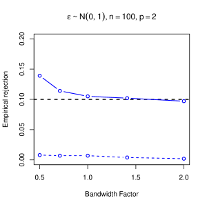
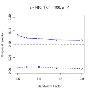
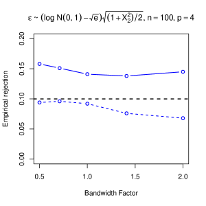
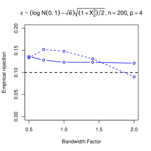
Figure 1: Empirical rejections under $H_{0}$ as a function of the bandwidth

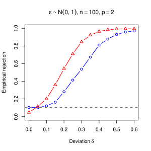
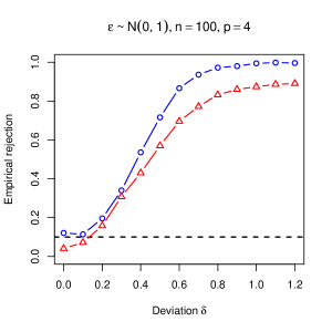
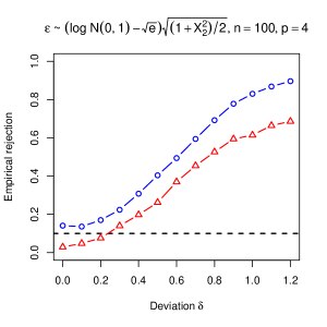
Figure 2: Power curves for model (V.11), $n=100$

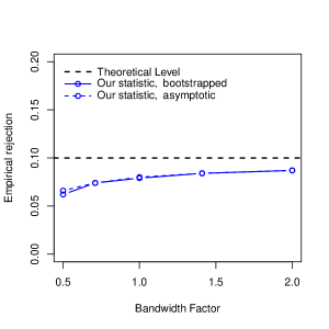
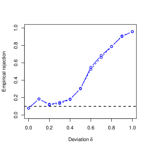
Figure 3: Empirical rejections under $H_{0}$ and $H_{1}$ for conditional law, $n=200$. On the left part, $h=c\times n^{-2/9}$ with varying $c$. On the right part, $Y=\left(1-\delta\right)\mathcal{N}\left(X^{\prime}\beta,\,0.09\right)+\delta\mathcal{N}\left(\left\|X\right\|,\,0.09\right)$.

VI Conclusions and furthers extensions

We have constructed new smoothing-based test procedures for SIM hypotheses for mean regression and for conditional law. Smoothing is only used on the estimated index, and the corresponding test statistics are asymptotically standard normal. A quite effective wild bootstrap procedure allows to correct the critical values with small samples. For simplicity we focused on univariate responses but, with obvious adjustments, our approach also applies to the case of multivariate responses. See Picone and Butler (2000) and Chen and Van Keilegom (2009) for more general situations with multivariate responses where our test methodology applies. Moreover, our statistics directly generalize to test multiple index against fully nonparametric alternatives. It suffice to consider the general methodology presented in section III with $q$ equal to the number of indices. Some other possible extensions that would require additional, though quite straightforward, investigation are the goodness-of-fit checks of index quantile regressions, see Kong and Xia (2012), and the functional index models, see Chen et al. (2011). Such extensions are left for future work.

VII Appendix 1: assumptions and proofs

Let $\mathcal{H}$ be the real line or the Hilbert space of squared integrable functions defined on $[0,1].$ Let $\langle\cdot,\cdot\rangle_{\mathcal{H}}$ and $\|\cdot\|_{\mathcal{H}}$ denote the associated inner product and norm. For an observation $(Y_{i},X_{i}^{\prime})^{\prime},$ $Y_{i}\in\mathbb{R}$ and $X_{i}\in\mathbb{R}^{p},$ let $Y_{i}(t)\equiv Y_{i}$ or $Y_{i}(t)=\mathbf{1}\{Y_{i}\leq\Phi^{-1}(t)\},$ and for any $\beta$ in the parameter set $\mathcal{B}\subset\mathbb{R}^{p},$ let $r_{i}(t;{\beta})=\mathbb{E}[Y_{i}(t)\mid Z_{i}({\beta})],$ $t\in[0,1].$ Thus, $Y_{i}(\cdot)$ is an element of $\mathcal{H}.$

Let $(\epsilon_{i}(\cdot),X_{i}^{\prime})^{\prime},$ $1\leq i\leq n,$ be random variables such that $\epsilon_{i}(\cdot)\in\mathcal{H}$ and $X_{i}\in\mathbb{R}^{p}.$ Let $\bar{\beta}$ be some element in the parameter set $\mathcal{B}.$ Consider $r_{i}(t;\bar{\beta})$ that depends only on $Z_{i}(\bar{\beta})=X_{i}^{\prime}\bar{\beta}$ and $\delta(X_{i},t)$ be such that $\mathbb{E}[\delta(X_{i},t)\mid Z_{i}(\bar{\beta})]=0,$ $t\in[0,1].$ Define

$$Y_{ni}(t)=r_{i}(t;\bar{\beta})+r_{n}\delta(X_{i},t)+\epsilon_{i}(t),\qquad t\in[0,1],1\leq i\leq n,$$

where $r_{n},$ $n\geq 1,$ is some bounded sequence of real numbers. In particular that means $\mathbb{E}[Y_{ni}(\cdot)\mid Z_{i}(\bar{\beta})]=r_{i}(\cdot;\bar{\beta}).$ The case of a null sequence $(r_{n})$ corresponds to the null hypothesis, while a sequence tending to zero corresponds to Pitman alternatives.

Assumption VII.1

a) The random variables $(\epsilon_{i}(\cdot),X_{i}^{\prime})^{\prime},$ $1\leq i\leq n,$ are independent copies of $\epsilon(\cdot)\in\mathcal{H}$ and $X\in\mathbb{R}^{p}.$ Moreover, $X^{\prime}\bar{\beta}$ admits a bounded density $f_{\bar{\beta}}.$

b) $\mathbb{E}[\exp(\rho\|X_{i}\|)]<\infty$ for some $\rho>0$ and $\mathbb{E}[\sup_{t}|r_{i}(t;\bar{\beta})+\epsilon_{i}(t)|^{a}]<\infty$ for some $a>8.$ Moreover, $\mathbb{E}(\|\epsilon_{i}(\cdot)\|^{2}_{\mathcal{H}}\mid X_{i})$ is bounded.

c) For any $t\in[0,1],$ the map $v\mapsto\mathbb{E}[Y_{ni}(t)\mid Z_{i}(\bar{\beta})=v]$ is twice differentiable. The second derivative $r_{i}^{\prime\prime}(\cdot;\bar{\beta})$ is uniformly Lipschitz (that is the Lipschitz constant independent of $t$) and uniformly bounded, while the first derivative satisfies $\mathbb{E}[\|r_{i}^{\prime}(\cdot;\bar{\beta})\|_{\mathcal{H}}^{4}]<\infty.$

d) The function $f_{\bar{\beta}}(\cdot)$ is uniformly Lipschitz.

e) The function $\delta(\cdot,\cdot)$ is bounded.

f) The kernels $K$ and $L$ are symmetric integrable functions, differentiable except at most a finite set of points and $L^{\prime}$ is Lipschitz continuous. Moreover, $\int_{\mathbb{R}}|L(t)|dt=\int|K(t)|dt=1$ and $\int_{\mathbb{R}}(|L^{\prime}(t)|+|K^{\prime}(t)|)dt<\infty.$ The map $v\mapsto|L^{\prime}(v)|/v$ is bounded in a neighborhood of the origin, $v^{2}K(v)\rightarrow 0$ if $v\rightarrow\infty,$ and $\int v^{2}\{|L(v)|+|K(v)|\}dv<\infty.$ Moreover, the Fourier Transform $\mathcal{F}[K]$ is positive on the real line.

g) The bandwidths satisfy the conditions $g,h\rightarrow 0$, $h/g^{2}\rightarrow 0,$ $nh^{1/2}g^{4}\rightarrow 0,$ $r_{n}^{2}nh^{1/2}\rightarrow\infty.$ Moreover, $g=n^{-\gamma}$ with $\gamma\in(1/5,1/4)$ and thus $nh^{2}\rightarrow\infty.$

Proof Proposition 4.1. First let us remark that for any $(a_{n}),$ a sequence divergent to infinity,

$$\mathbb{P}\left(\max_{1\leq i\leq n}\|X_{i}\|>a_{n}\ln n\right)\rightarrow 0\quad\text{and}\quad\mathbb{P}\left(\|\beta_{n}-\bar{\beta}\|>a_{n}n^{-1/2}\right)\rightarrow 0.$$ (VII.1)

Moreover, at least for $\beta$ in a fixed but small enough neighborhood of $\bar{\beta}$, the matrix $\mathbf{A}\left(\beta\right)$ could be built such that the norm of each of the $p-1$ columns of $\mathbf{A}\left(\beta\right)-\mathbf{A}\left(\bar{\beta}\right)$ is bounded by $c\|\beta_{n}-\bar{\beta}\|$ with $c$ a constant independent of $\beta$. Indeed, one could consider $p-1$ independent vectors which completed by any $\beta$ close to $\bar{\beta}$ form a basis. Then one could use the Gram-Schmidt procedure to orthonormalize the basis. By construction, the norm of any columns of $\mathbf{A}\left(\beta\right)-\mathbf{A}\left(\bar{\beta}\right)$ is bounded by $c\|\beta_{n}-\bar{\beta}\|$ for some $c$ depending only on the initial $p-1$ independent vectors. All these facts show that we can reduce the parameter set to $\mathcal{B}_{n},$ $n\geq 1,$ a sequence of balls centered at $\bar{\beta}$ of radius converging to zero. Consider the set of elementary events

$$\mathcal{E}_{n}=\left\{\max_{1\leq i\leq n}\sup_{\beta\in\mathcal{B}_{n}}[\|Z_{i}(\beta)-Z_{i}(\bar{\beta})\|+\|W_{i}(\beta)-W_{i}(\bar{\beta})\|]\leq b_{n}\right\},$$ (VII.2)

where $b_{n}$ is a sequence such that $b_{n}\rightarrow 0.$ The equation (VII.1) indicates that the sequences $\mathcal{B}_{n}$ and $b_{n}$ could be taken such that the radius of $\mathcal{B}_{n}$ converges to zero slower than $n^{-1/2}$ and faster than $b_{n},$ and $b_{n}n^{1/2}/\ln n\rightarrow\infty.$ Then $\mathbb{P}(\beta_{n}\in\mathcal{B}_{n})\rightarrow 1$ and $\mathbb{P}(\mathcal{E}_{n}^{c})$ decreases to zero faster than any negative power of the sample size $n.$ Hence, in the following it will suffices to prove the statements on the set $\{\beta_{n}\in\mathcal{B}_{n}\}\cap\mathcal{E}_{n}.$

We will focus on $I_{n}(\beta_{n})$ since the arguments for $\hat{\omega}(\beta_{n})$ are similar and much simpler. Hereafter, by abuse, we write $Y_{i}(t)$ instead of $Y_{ni}(t)$ even when $r_{n}\neq 0.$ To prove that $I_{n}({\beta_{n}})-I_{n}(\bar{\beta})=o_{\mathbb{P}}(I_{n}(\bar{\beta}))$ we will show below that $I_{n}({\beta_{n}})-I_{n}(\bar{\beta})=o_{\mathbb{P}}(n^{-1}h^{-1/2}+r_{n}^{2}).$ This shows that $I_{n}({\beta_{n}})$ is negligible compared to $I_{n}(\bar{\beta})$ both on the null and alternative hypotheses. Indeed, under the null hypothesis, $r_{n}\equiv 0,$ $\bar{\beta}=\beta_{0}$ and $nh^{1/2}I_{n}({\beta_{0}})$ is asymptotically centered normal distributed, while on the alternative the $I_{n}(\bar{\beta})$ is driven by a term of order $r_{n}^{2}.$

In the following $C,$ $C^{\prime}$,… denote constants that may have different values from line to line. Let us simplify notation and write

$$\widehat{V}_{i}(\beta)=\widehat{U_{i}w(Z_{i})}(\beta)$$

and

$$L_{ij}(\beta)=L_{ij}(\beta,g),\;K_{ij}(\beta)=K_{ij}(\beta,h),\;\phi_{ij}(\beta)=\phi(W_{i}({\beta})-W_{j}({\beta})).$$ (VII.3)

Then,

$$I_{n}({\beta})-I_{n}({\bar{\beta}})\!\! = \!\!\dfrac{1}{n(n-1)h}\sum_{i\neq j}\!\!\left[\left\langle\widehat{V}_{i}(\beta),\;\widehat{V}_{j}(\beta)\right\rangle_{\mathcal{H}}\!-\left\langle\widehat{V}_{i}(\bar{\beta}),\;\widehat{V}_{j}(\bar{\beta})\right\rangle_{\mathcal{H}}\right]K_{ij}({\bar{\beta}})\phi_{ij}(\bar{\beta})$$

$$+ \!\!\dfrac{1}{n(n-1)h}\sum_{i\neq j}\!\!\left\langle\widehat{V}_{i}(\bar{\beta}),\;\widehat{V}_{j}(\bar{\beta})\right\rangle_{\mathcal{H}}\left[K_{ij}({\beta})\phi_{ij}(\beta)-K_{ij}({\bar{\beta}})\phi_{ij}(\bar{\beta})\right]$$

$$+ \dfrac{1}{n(n-1)h}\sum_{i\neq j}\!\!\left[\left\langle\widehat{V}_{i}(\beta),\;\widehat{V}_{j}(\beta)\right\rangle_{\mathcal{H}}\!-\left\langle\widehat{V}_{i}(\bar{\beta}),\;\widehat{V}_{j}(\bar{\beta})\right\rangle_{\mathcal{H}}\right]$$

$$\qquad\qquad\qquad\qquad\qquad\qquad\times\left[K_{ij}({\beta})\phi_{ij}(\beta)-K_{ij}({\bar{\beta}})\phi_{ij}(\bar{\beta})\right]$$

$$= D_{n1}(\beta)+D_{n2}(\beta)+D_{n3}(\beta).$$

Let us investigate the uniform rates of $D_{n1}$ and $D_{n2}$, the term $D_{n3}$ being uniformly smaller. We can write

$$D_{n1}(\beta) = \dfrac{2}{n(n-1)h}\sum_{i\neq j}\left\langle\widehat{V}_{i}(\beta)-\widehat{V}_{i}(\bar{\beta}),\;\widehat{V}_{j}(\bar{\beta})\right\rangle_{\mathcal{H}}K_{ij}({\bar{\beta}})\phi_{ij}(\bar{\beta})$$

$$+\dfrac{1}{n(n-1)h}\sum_{i\neq j}\left\langle\widehat{V}_{i}(\beta)-\widehat{V}_{i}(\bar{\beta}),\;\widehat{V}_{j}(\beta)-\widehat{V}_{j}(\bar{\beta})\right\rangle_{\mathcal{H}}K_{ij}({\bar{\beta}})\phi_{ij}(\bar{\beta})$$

$$= 2D_{n11}(\beta)+D_{n12}(\beta).$$

Moreover,

$$\widehat{V}_{i}(\bar{\beta})(t) = \frac{1}{n-1}\sum\limits_{k\neq i}[Y_{i}(t)-Y_{k}(t)]\frac{1}{g}L_{ik}(\bar{\beta})$$

$$= [Y_{i}(t)-r_{i}(t;\bar{\beta})]f_{\bar{\beta}}(X_{i}^{\prime}\bar{\beta})$$

$$+[Y_{i}(t)-r_{i}(t;\bar{\beta})]\left[\frac{1}{n-1}\sum\limits_{k\neq i}\frac{1}{g}L_{ik}(\bar{\beta})-f_{\bar{\beta}}(X_{i}^{\prime}\bar{\beta})\right]$$

$$+\frac{1}{n-1}\sum\limits_{k\neq i}\{r_{i}(t;\bar{\beta})-r_{k}(t;\bar{\beta})\}\frac{1}{g}L_{ik}(\bar{\beta})$$

$$-\frac{1}{n-1}\sum\limits_{k\neq i}\{Y_{k}(t)-r_{k}(t;\bar{\beta})\}\frac{1}{g}L_{ik}(\bar{\beta})$$

$$= [Y_{i}(t)-r_{i}(t;\bar{\beta})]f_{\bar{\beta}}(X_{i}^{\prime}\bar{\beta})+[Y_{i}(t)-r_{i}(t;\bar{\beta})]R_{1,ni}+R_{2,ni}(t)-R_{3,ni}(t),$$

where, by Lemma 8.2

$$\sup_{1\leq i\leq n}\!\!|R_{1,ni}|=O_{\mathbb{P}}(g+n^{-1/2}g^{-1/2}\ln^{1/2}n),$$

and, Lemma 8.1 yields

$$\sup_{1\leq i\leq n}\sup_{t\in[0,1]}|R_{3,ni}(t)|=O_{\mathbb{P}}(n^{-1/2}g^{-1/2}\ln^{1/2}n).$$

A representation of $R_{2,ni}(t)$ is provided in Lemma 8.3. On the other hand,

$$\widehat{V}_{i}(\beta)(t)-\widehat{V}_{i}(\bar{\beta})(t) = \frac{1}{n-1}\sum\limits_{k\neq i}[Y_{i}(t)-Y_{k}(t)]\left[\frac{1}{g}L_{ik}(\beta)-\frac{1}{g}L_{ik}(\bar{\beta})\right].$$

Uniform bounds for $D_{n1}.$

The rate of $D_{n11}.$ Since $Y_{i}(t)=r_{i}(t;\bar{\beta})+r_{n}\delta(X_{i},t)+\epsilon_{i}(t),$ with $\mathbb{E}[\epsilon_{i}(t)\mid X_{i}]=0,$ we have $D_{n11}(\beta)=D_{n111}(\beta)+R_{n11}(\beta)$ with

$$D_{n111}(\beta) = \dfrac{1}{n(n-1)^{2}h}\sum_{i\neq j\neq k}\left\langle Y_{i}(\cdot)-Y_{k}(\cdot),\;Y_{j}(\cdot)-r_{j}(\cdot;\bar{\beta})\right\rangle_{\mathcal{H}}f_{\bar{\beta}}(X_{j}^{\prime}\bar{\beta})$$

$$\qquad\qquad\qquad\qquad\qquad\times\left[\frac{1}{g}L_{ik}(\beta)-\frac{1}{g}L_{ik}(\bar{\beta})\right]K_{ij}({\bar{\beta}})\phi_{ij}(\bar{\beta})$$

$$= \dfrac{1}{n(n-1)^{2}h}\sum_{i\neq j\neq k}\left\langle Y_{i}(\cdot)-Y_{k}(\cdot),\;\epsilon_{j}(\cdot)\right\rangle_{\mathcal{H}}f_{\bar{\beta}}(X_{j}^{\prime}\bar{\beta})$$

$$\qquad\qquad\qquad\qquad\qquad\times\left[\frac{1}{g}L_{ik}(\beta)-\frac{1}{g}L_{ik}(\bar{\beta})\right]K_{ij}({\bar{\beta}})\phi_{ij}(\bar{\beta}),$$

and $R_{n11}(\beta)=D_{n11}(\beta)-D_{n111}(\beta).$ We decompose

$$D_{n111}(\beta) = \dfrac{1}{n(n-1)^{2}h}\sum_{i\neq j\neq k}\left\langle\epsilon_{i}(\cdot)-\epsilon_{k}(\cdot),\;\epsilon_{j}(\cdot)\right\rangle_{\mathcal{H}}f_{\bar{\beta}}(X_{j}^{\prime}\bar{\beta})$$

$$\qquad\qquad\qquad\times\left[\frac{1}{g}L_{ik}(\beta)-\frac{1}{g}L_{ik}(\bar{\beta})\right]K_{ij}({\bar{\beta}})\phi_{ij}(\bar{\beta})$$

$$+\dfrac{1}{n(n-1)^{2}h}\sum_{i\neq j\neq k}\left\langle r_{i}(\cdot;\bar{\beta})-r_{k}(\cdot;\bar{\beta}),\;\epsilon_{j}(\cdot)\right\rangle_{\mathcal{H}}f_{\bar{\beta}}(X_{j}^{\prime}\bar{\beta})$$

$$\qquad\qquad\qquad\times\left[\frac{1}{g}L_{ik}(\beta)-\frac{1}{g}L_{ik}(\bar{\beta})\right]K_{ij}({\bar{\beta}})\phi_{ij}(\bar{\beta})$$

$$+\dfrac{r_{n}}{n(n-1)^{2}h}\sum_{i\neq j\neq k}\left\langle\delta(X_{i},t)-\delta(X_{k},t),\;\epsilon_{j}(\cdot)\right\rangle_{\mathcal{H}}f_{\bar{\beta}}(X_{j}^{\prime}\bar{\beta})$$

$$\qquad\qquad\qquad\times\left[\frac{1}{g}L_{ik}(\beta)-\frac{1}{g}L_{ik}(\bar{\beta})\right]K_{ij}({\bar{\beta}})\phi_{ij}(\bar{\beta})$$

$$= D_{n1111}(\beta)+D_{n1112}(\beta)+r_{n}D_{n1113}(\beta).$$

The quantity $ghD_{n1111}(\beta)$ could be decomposed in a sum of degenerate $U-$process of order 3 and another one of order 2 indexed by $\beta.$ To bound them we use the maximal inequality of Sherman (1994). Since $nh^{2},ng^{4}\rightarrow\infty,$ deduce that the degenerate $U-$process of order 3 is of uniform rate

$$n^{-3/2}O_{\mathbb{P}}(h^{\alpha/2}\{b_{n}^{2}g^{-1}\}^{\alpha/2})=gh\times o_{\mathbb{P}}(n^{-1}h^{-1/2}),$$

over any sequence of balls centered at $\bar{\beta}$ with radius decreasing to zero faster than $b_{n},$ where $b_{n}$ is a sequence such that $b_{n}n^{1/2}/\ln n\rightarrow\infty$ and $\alpha$ could be a number in the interval $(0,1)$ arbitrarily close to 1. The details on how the maximal inequality of Sherman (1994) applies are provided below for deriving the uniform rate of $D_{n12}.$ To bound the right-hand side term in that maximal inequality we use the fact that $\mathbb{E}(\|\epsilon\|_{\mathcal{H}}^{2}\mid X)$ and $f_{\bar{\beta}}(X^{\prime}\bar{\beta})$ are bounded and the uniform bounds (VIII.6), (VIII.4) and (VIII.5) from Lemma 8.4 in the Appendix. Using very similar arguments, the degenerate $U-$process of order 2 in the decomposition of $ghD_{n1111}(\beta)$ could be shown to be of uniform rate

$$n^{-1}O_{\mathbb{P}}(h^{\alpha/2}\{b_{n}^{2}g^{-1}\}^{\alpha/2})=gh\times o_{\mathbb{P}}(n^{-1}h^{-1/2})$$

provided that $nh^{2},ng^{4}\rightarrow\infty$ and $\alpha$ is sufficiently close to 1. Next, for $ngD_{n1112}(\beta),$ that is centered, use the Hoeffding decomposition and the regularity of the function $v\mapsto\mathbb{E}[Y(t)\mid Z(\bar{\beta})=v].$ For the degenerate $U-$processes of order 3 and 2 in the Hoeffding decomposition of $D_{n1112}(\beta)$ we apply the maximal inequality of Sherman (1994) as previously. Deduce the respective uniform rates over $\mathcal{B}_{n}$

$$g^{2}n^{-3/2}O_{\mathbb{P}}(h^{\alpha/2}\{b_{n}^{2}g^{-1}\}^{\alpha/2})=gh\times o_{\mathbb{P}}(n^{-1}h^{-1/2}),$$

and

$$g^{2}n^{-1}O_{\mathbb{P}}(h^{\alpha/2}\{b_{n}^{2}g^{-1}\}^{\alpha/2})=gh\times o_{\mathbb{P}}(n^{-1}h^{-1/2}).$$

It remains the $U-$process of order 1. Using again the bounds from Lemma 8.4, deduce the uniform rate over $\mathcal{B}_{n}$

$$g^{2}n^{-1/2}O_{\mathbb{P}}(h^{\alpha}\{b_{n}^{2}g^{-1}\}^{\alpha/2})=gh\times o_{\mathbb{P}}(n^{-1}h^{-1/2}).$$

Deduce $D_{n1112}(\beta_{n})=o_{\mathbb{P}}(n^{-1}h^{-1/2}).$ For $ghD_{n1113}(\beta)$ the arguments are similar, but without the $g^{2}$ factor, and yield the uniform rate

$$n^{-1/2}O_{\mathbb{P}}(h^{\alpha}\{b_{n}^{2}g^{-1}\}^{\alpha/2})=gh\times o_{\mathbb{P}}(n^{-1}h^{-1/2})=o_{\mathbb{P}}(n^{-1/2}h^{-1/4}),$$

provided $nh^{2},ng^{4}\rightarrow\infty$ and $\alpha$ is sufficiently close to 1. Deduce that $D_{n111}(\beta_{n})=o_{\mathbb{P}}(n^{-1}h^{-1/2}+r_{n}^{2}).$

For $R_{n11}(\beta)$ we can write

$$R_{n11}(\beta) = \dfrac{1}{n(n-1)^{2}h}\sum_{i\neq j}\left\langle Y_{i}(\cdot)-Y_{j}(\cdot),\;Y_{j}(\cdot)-r_{j}(t;\bar{\beta})\right\rangle_{\mathcal{H}}f_{\bar{\beta}}(X_{j}^{\prime}\bar{\beta})$$

$$\qquad\qquad\qquad\times\left[\frac{1}{g}L_{ij}(\beta)-\frac{1}{g}L_{ij}(\bar{\beta})\right]K_{ij}({\bar{\beta}})\phi_{ij}(\bar{\beta})$$

$$+\dfrac{1}{n(n-1)^{2}h}\sum_{i\neq j,i\neq k}\left\langle Y_{i}(\cdot)-Y_{k}(\cdot),\;Y_{j}(\cdot)-r_{j}(t;\bar{\beta})\right\rangle_{\mathcal{H}}R_{1,nj}$$

$$\qquad\qquad\qquad\times\left[\frac{1}{g}L_{ik}(\beta)-\frac{1}{g}L_{ik}(\bar{\beta})\right]K_{ij}({\bar{\beta}})\phi_{ij}(\bar{\beta})$$

$$+\dfrac{1}{n(n-1)^{2}h}\sum_{i\neq j,i\neq k}\left\langle Y_{i}(\cdot)-Y_{k}(\cdot),\;R_{2,nj}(\cdot)+R_{3,nj}(\cdot)\right\rangle_{\mathcal{H}}$$

$$\qquad\qquad\qquad\times\left[\frac{1}{g}L_{ik}(\beta)-\frac{1}{g}L_{ik}(\bar{\beta})\right]K_{ij}({\bar{\beta}})\phi_{ij}(\bar{\beta})$$

$$= R_{n111}(\beta)+R_{n112}(\beta)+R_{n113}(\beta).$$

We only investigate $R_{n111}(\beta)$, the terms $R_{n112}(\beta)$ and $R_{n113}(\beta)$ are uniformly smaller compared to $D_{n111}(\beta)$. We can write

$$R_{n111}(\beta) = \dfrac{1}{n-1}\;\dfrac{1}{n(n-1)h}\sum_{i\neq j}\left\langle\epsilon_{i}(\cdot)-\epsilon_{j}(\cdot),\;\epsilon_{j}(\cdot)\right\rangle_{\mathcal{H}}f_{\bar{\beta}}(X_{j}^{\prime}\bar{\beta})$$

$$\qquad\qquad\qquad\times\left[\frac{1}{g}L_{ij}(\beta)-\frac{1}{g}L_{ij}(\bar{\beta})\right]K_{ij}({\bar{\beta}})\phi_{ij}(\bar{\beta})$$

$$+\dfrac{1}{n-1}\;\dfrac{1}{n(n-1)h}\sum_{i\neq j}\left\langle r_{i}(\cdot;\bar{\beta})-r_{j}(\cdot;\bar{\beta}),\;\epsilon_{j}(\cdot)\right\rangle_{\mathcal{H}}f_{\bar{\beta}}(X_{j}^{\prime}\bar{\beta})$$

$$\qquad\qquad\qquad\times\left[\frac{1}{g}L_{ij}(\beta)-\frac{1}{g}L_{ij}(\bar{\beta})\right]K_{ij}({\bar{\beta}})\phi_{ij}(\bar{\beta})$$

$$+\dfrac{1}{n-1}\;\dfrac{r_{n}}{n(n-1)h}\sum_{i\neq j}\left\langle\delta(X_{i},t)-\delta(X_{j},t),\;\epsilon_{j}(\cdot)\right\rangle_{\mathcal{H}}f_{\bar{\beta}}(X_{j}^{\prime}\bar{\beta})$$

$$\qquad\qquad\qquad\times\left[\frac{1}{g}L_{ij}(\beta)-\frac{1}{g}L_{ij}(\bar{\beta})\right]K_{ij}({\bar{\beta}})\phi_{ij}(\bar{\beta})$$

$$= R_{n1111}(\beta)+R_{n1112}(\beta)+r_{n}R_{n1113}(\beta).$$

The leading term in $R_{n1111}(\beta)$ is

$$\dfrac{1}{n-1}\dfrac{1}{n(n-1)h}\sum_{i\neq j}\left\|\epsilon_{j}(\cdot)\right\|^{2}_{\mathcal{H}}f_{\bar{\beta}}(X_{j}^{\prime}\bar{\beta})\left[\frac{1}{g}L_{ij}(\beta)-\frac{1}{g}L_{ij}(\bar{\beta})\right]K_{ij}({\bar{\beta}})\phi_{ij}(\bar{\beta}).$$

Use the boundedness of $\mathbb{E}[\left\|\epsilon_{j}(\cdot)\right\|^{2}_{\mathcal{H}}\mid X_{j}]$ and $f_{\bar{\beta}}(X_{j}^{\prime}\bar{\beta}),$ and Lemma 8.4 to deduce that $R_{n1111}(\beta_{n})=o_{\mathbb{P}}(n^{-1}).$ Gathering facts deduce that

$$D_{n11}(\beta_{n})=o_{\mathbb{P}}(n^{-1}h^{-1/2}+r_{n}^{2}).$$

The rate of $D_{n12}.$ We have

$$\widehat{V}_{i}(\beta)(t)-\widehat{V}_{i}(\bar{\beta})(t)=Y_{i}(t)\Delta_{1,ni}(\beta)+\Delta_{2,ni}(\beta)$$

with $\Delta_{1,ni}(\beta)$ and $\Delta_{2,ni}(\beta)$ independent of $t$ and

$$\sup_{1\leq i\leq n}\sup_{\beta\in\mathcal{B}_{n}}\{|\Delta_{1,ni}|+|\Delta_{2,ni}|\}=O_{\mathbb{P}}(n^{-1/2}g^{-1/2}\ln^{1/2}n+b_{n});$$

see Lemma 8.1. Replacing and taking absolute values, deduce

$$D_{n12}(\beta_{n})=O_{\mathbb{P}}(n^{-1}g^{-1}\ln n+n^{-1}\ln^{2}n)=o_{\mathbb{P}}(n^{-1}h^{-1/2}),$$

since $g^{-1}h^{1/2}\rightarrow 0$ and $h\ln^{4}n\rightarrow 0.$

Gathering facts deduce that

$$D_{n1}(\beta_{n})=D_{n11}(\beta_{n})+D_{n12}(\beta_{n})=o_{\mathbb{P}}(n^{-1}h^{-1/2}+r_{n}^{2}).$$

Uniform bounds for $D_{n2}.$

We have

$$D_{n2}(\beta) = \dfrac{1}{n(n-1)h}\sum_{i\neq j}\!\!\left\langle\widehat{V}_{i}(\bar{\beta}),\;\widehat{V}_{j}(\bar{\beta})\right\rangle_{\mathcal{H}}\left[K_{ij}({\beta})\phi_{ij}(\beta)-K_{ij}({\bar{\beta}})\phi_{ij}(\bar{\beta})\right]$$

$$= \dfrac{1}{n(n-1)h}\sum_{i\neq j}\!\!\left\langle[Y_{i}(t)-r_{i}(t;\bar{\beta})]f_{\bar{\beta}}(X_{i}^{\prime}\bar{\beta}),\;[Y_{j}(t)-r_{j}(t;\bar{\beta})]f_{\bar{\beta}}(X_{j}^{\prime}\bar{\beta})\right\rangle_{\mathcal{H}}$$

$$\qquad\qquad\qquad\qquad\qquad\qquad\times\left[K_{ij}({\beta})\phi_{ij}(\beta)-K_{ij}({\bar{\beta}})\phi_{ij}(\bar{\beta})\right]$$

$$+\text{terms of smaller rate}$$

$$= D_{n21}(\beta)+\text{terms of smaller rate}.$$

Recall that by construction,

$$\mathbb{E}[Y_{i}(t)\mid X_{i}]=r_{i}(t;\bar{\beta})+r_{n}\delta(X_{i},t),$$

so that

$$[Y_{i}(t)-r_{i}(t;\bar{\beta})]f_{\bar{\beta}}(X_{i}^{\prime}\bar{\beta})=[\epsilon_{i}(t)+r_{n}\delta(X_{i},t)]f_{\bar{\beta}}(X_{i}^{\prime}\bar{\beta}),$$

with $\mathbb{E}[\epsilon_{i}(t)\mid X_{i}]=0,$ $\forall t\in[0,1].$ Thus

$$D_{n21}(\beta)=\dfrac{1}{n(n-1)h}\sum_{i\neq j}\!\!\left\langle\epsilon_{i}(t),\;\epsilon_{j}(t)\right\rangle_{\mathcal{H}}f_{\bar{\beta}}(X_{i}^{\prime}\bar{\beta})f_{\bar{\beta}}(X_{j}^{\prime}\bar{\beta})\left[K_{ij}({\beta})\phi_{ij}(\beta)-K_{ij}({\bar{\beta}})\phi_{ij}(\bar{\beta})\right]\\ +\dfrac{2r_{n}}{n(n-1)h}\sum_{i\neq j}\!\left\langle\epsilon_{i}(t),\;\delta(X_{j},t)\right\rangle_{\mathcal{H}}f_{\bar{\beta}}(X_{i}^{\prime}\bar{\beta})f_{\bar{\beta}}(X_{j}^{\prime}\bar{\beta})\left[K_{ij}({\beta})\phi_{ij}(\beta)-K_{ij}({\bar{\beta}})\phi_{ij}(\bar{\beta})\right]\\ +\dfrac{r^{2}_{n}}{n(n-1)h}\sum_{i\neq j}\!\left\langle\delta(X_{i},t),\;\delta(X_{j},t)\right\rangle_{\mathcal{H}}f_{\bar{\beta}}(X_{i}^{\prime}\bar{\beta})f_{\bar{\beta}}(X_{j}^{\prime}\bar{\beta})\left[K_{ij}({\beta})\phi_{ij}(\beta)-K_{ij}({\bar{\beta}})\phi_{ij}(\bar{\beta})\right]\\ =D_{n211}(\beta)+2r_{n}D_{n212}(\beta)+r_{n}^{2}D_{n213}(\beta).$$

The term $D_{n211}(\cdot)$ is a degenerate $U-$process of order 2, indexed by $\beta$. Consider the family of functions

$$\mathcal{F}_{n}=\{h(\cdot,\cdot;\beta):\beta\in\mathcal{B}_{n}\}$$ (VII.4)

with

$$h((x_{1},\epsilon_{1}),(x_{2},\epsilon_{2});\beta)=\langle\epsilon_{1}(\cdot),\;\epsilon_{2}(\cdot)\rangle_{\mathcal{H}}f_{\bar{\beta}}(x_{1}^{\prime}\bar{\beta})f_{\bar{\beta}}(x_{2}^{\prime}\bar{\beta})[K_{12}(\beta)\phi_{12}(\beta)-K_{12}(\bar{\beta})\phi_{12}(\bar{\beta})].$$

It is quite easy to see that $\mathcal{F}_{n}$ is a VC class, or Euclidean in the terminology of Sherman (1994), for a squared integrable envelope $H(\cdot),$ with some $A$ and $V$ independent of $n$. (Recall that the $\delta-$covering number of an Euclidean class of function is bounded by $A\delta^{-V}$.) Since $\mathbb{E}(\|\epsilon_{1}(\cdot)\|^{2}_{\mathcal{H}}\mid X_{1})$ and $f_{\bar{\beta}}(X_{1}^{\prime}\bar{\beta})$ are bounded, and the kernel $K$ is bounded, by Lemma 8.4 deduce that

$$\mathbb{E}\left[\sup_{\beta\in\mathcal{B}_{n}}h(\cdot,\cdot;\beta)^{2}\right]\leq Ch^{1/2}b_{n}$$

for some constant $C>0$ independent on $n$ and $\bar{\beta}$. See Lemma 8.4 below. Applying the Main Corollary of Sherman (1994) with $k=2,$ $p=1$, deduce that

$$\sup_{\beta}|hD_{n211}(\beta)|\leq\frac{C^{\prime}}{n}(b_{n}h^{1/2})^{\alpha/2}=n^{-1}h^{1/2}\times O(n^{-\alpha/4}h^{\alpha/4-1/2})$$

for $0<\alpha<1$. Since and $\alpha$ could be arbitrarily close to 1 and $b_{n}$ could be any sequence such that $b_{n}n^{1/2}\ln^{-1}n\rightarrow\infty$ and $nh^{3/2}\rightarrow 0,$ deduce that

$$D_{n211}(\beta_{n})=o_{\mathbb{P}}(n^{-1}h^{-1/2}).$$

For the uniform rate of the centered $U-$process $D_{n212}(\cdot),$ use the Hoeffding decomposition. The degenerate $U-$process of order 1 in this decomposition could be handled with the arguments used for $D_{n211}(\cdot)$ and shown to be of uniform rate $o_{\mathbb{P}}(n^{-1/2})$. The degenerate $U-$process of order 2 in the decomposition is

$$D_{n212,1}(\beta)=\dfrac{1}{n}\sum_{i\neq j}\!\left\langle\epsilon_{i}(t),\;\gamma_{i}(\beta,t;h)\right\rangle_{\mathcal{H}}f_{\bar{\beta}}(X_{i}^{\prime}\bar{\beta})$$

where

$$\gamma_{i}(\beta,t;h)=\mathbb{E}\left\{\delta(X_{j},t)f_{\bar{\beta}}(X_{j}^{\prime}\bar{\beta})h^{-1}\left[K_{ij}({\beta})\phi_{ij}(\beta)-K_{ij}({\bar{\beta}})\phi_{ij}(\bar{\beta})\right]\mid X_{i}\right\}.$$

Since $f_{\bar{\beta}}$ and $\delta(X,\cdot)$ are supposed bounded, arguments as used for Lemma 8.4 allow to show that $\mathbb{E}[\sup_{\beta}\gamma^{2}_{i}(\beta,t)]=o(1).$ Deduce that $D_{n212,1}(\beta_{n})=o_{\mathbb{P}}(n^{-1/2}).$ Gathering facts, $r_{n}D_{n212}(\beta_{n})$ is negligible compared to $r_{n}^{2}.$ By the same arguments, $D_{n213}(\beta_{n})=o_{\mathbb{P}}(1)$ so that we can conclude that $D_{n2}(\beta_{n})=o_{\mathbb{P}}(n^{-1}h^{-1/2}+r_{n}^{2}).$  

Proof of Proposition 4.2. Let us consider the simplified notation from equation (VII.3) and further simplify in the case $\beta=\beta_{0}$ and write

$$L_{ij}=L_{ij}(\beta_{0},g),\quad K_{ij}=K_{ij}(\beta_{0},h),\quad\text{and}\quad\phi_{ij}=\phi(W_{i}(\beta_{0})-W_{j}(\beta_{0})).$$ (VII.5)

Notice that

$$I_{n}^{\{l\}}\left(\beta_{0}\right) = \dfrac{1}{n\left(n-1\right)h}\sum_{1\leq i\neq j\leq n}\left\{\left\langle\left(r_{i}-\tilde{r}_{i}\right)\left(\cdot;\,\beta_{0}\right),\,\left(r_{j}-\tilde{r}_{j}\right)\left(\cdot;\,\beta_{0}\right)\right\rangle_{L^{2}}\right.$$

$$\hphantom{\dfrac{1}{n\left(n-1\right)h}\sum_{1\leq i\neq j\leq n}\quad}+\left.\left\langle\epsilon_{i}\left(\cdot\right),\,\epsilon_{j}\left(\cdot\right)\right\rangle_{L^{2}}\right.$$

$$\hphantom{\dfrac{1}{n\left(n-1\right)h}\sum_{1\leq i\neq j\leq n}\quad}+\left.\left\langle\tilde{\epsilon}_{i}\left(\cdot\right),\,\tilde{\epsilon}_{j}\left(\cdot\right)\right\rangle_{L^{2}}\right.$$

$$\hphantom{\dfrac{1}{n\left(n-1\right)h}\sum_{1\leq i\neq j\leq n}\quad}+\left.2\left\langle\epsilon_{i}\left(\cdot\right),\,\left(r_{j}-\tilde{r}_{j}\right)\left(\cdot;\,\beta_{0}\right)\right\rangle_{L^{2}}\right.$$

$$\hphantom{\dfrac{1}{n\left(n-1\right)h}\sum_{1\leq i\neq j\leq n}\quad}-\left.2\left\langle\tilde{\epsilon}_{i}\left(\cdot\right),\,\left(r_{j}-\tilde{r}_{j}\right)\left(\cdot;\,\beta_{0}\right)\right\rangle_{L^{2}}\right.$$

$$\hphantom{\dfrac{1}{n\left(n-1\right)h}\sum_{1\leq i\neq j\leq n}\quad}-\left.2\left\langle\epsilon_{i}\left(\cdot\right),\,\tilde{\epsilon}_{j}\left(\cdot\right)\right\rangle_{L^{2}}\right\}\hat{f}_{\beta_{0},i}\hat{f}_{\beta_{0},j}K_{ij}\phi_{ij}$$

$$= I_{1}\left(\beta_{0}\right)+I_{2}\left(\beta_{0}\right)+I_{3}\left(\beta_{0}\right)+2I_{4}\left(\beta_{0}\right)-2I_{5}\left(\beta_{0}\right)-2I_{6}\left(\beta_{0}\right)$$

with

$$\hat{f}_{\beta,i}=\dfrac{1}{\left(n-1\right)g}\sum_{k\neq i}L_{ik}\left(\beta\right),\quad r_{i}\left(t;\,\beta\right)=\mathbb{P}\left[Y_{i}\leq\Phi^{-1}\left(t\right)\mid X_{i}^{\prime}\beta\right],$$

$$\tilde{r}_{i}\left(t;\,\beta\right)=\dfrac{1}{\left(n-1\right)g\hat{f}_{\beta,i}}\sum_{k\neq i}r_{k}\left(t;\,\beta\right)L_{ik}\left(\beta\right)$$

and $\tilde{\epsilon}_{i}\left(\cdot\right)$ is defined as $\tilde{r}_{i}\left(t;\,\beta\right)$ by replacing $r_{i}\left(t;\,\beta\right)$ by $\epsilon_{i}\left(\cdot\right)$. This decomposition of $I_{n}^{\{l\}}\left(\beta_{0}\right)$ is given by the identity

$$\widehat{U_{i}\omega\left(Z_{i}\right)}\left(\cdot;\,\beta_{0}\right)=\left[r_{i}\left(\cdot;\,\beta_{0}\right)-\tilde{r}_{i}\left(\cdot;\,\beta_{0}\right)+\epsilon_{i}\left(\cdot\right)-\tilde{\epsilon}_{i}\left(\cdot\right)\right]\hat{f}_{\beta_{0},i}.$$

The terms $I_{1}\left(\beta_{0}\right)$ and $I_{3}\left(\beta_{0}\right)$ are treated in Lemmas 8.6 and 8.7 in Section VIII. For $I_{2}\left(\beta_{0}\right)$, let us introduce

$$\omega_{n}^{2}\left(\beta\right)=\dfrac{2}{n\left(n-1\right)h}\sum_{i=1}^{n}\sum_{j\neq i}\intop\intop\Gamma^{2}\left(s,t\right)ds\,dt\,\hat{f}_{\beta,i}^{2}\hat{f}_{\beta,j}^{2}K_{ij}^{2}\left(\beta\right)\phi_{ij}^{2}\left(\beta\right).$$

Proposition 7.1 below ensures that $nh^{1/2}\omega_{n}^{-1}\left(\beta_{0}\right)I_{2}\left(\beta_{0}\right)\to\mathcal{N}\left(0,1\right)$ in law. The terms $I_{4}\left(\beta_{0}\right)$, $I_{5}\left(\beta_{0}\right)$ and $I_{6}\left(\beta_{0}\right)$ can be shown to be negligible in a similar way as $I_{1}\left(\beta_{0}\right)$ and $I_{3}\left(\beta_{0}\right)$. Lemma 8.9 shows that $\omega_{n}^{2}\left(\beta_{0}\right)\rightarrow\omega^{2}\left(\beta_{0}\right)$ in probability with $\omega^{2}\left(\beta_{0}\right)>0$ and thus $I_{j}\left(\beta_{0}\right)/\omega_{n}\left(\beta_{0}\right)$ is of the same order as $I_{j}\left(\beta_{0}\right)$ for $j\in\left\{1,3,4,5,6\right\}$. Finally, it is easy to check that $\omega_{n}\left(\beta_{0}\right)-\hat{\omega}_{n}^{\{l\}}\left(\beta_{0}\right)=o_{\mathbb{P}}(1).$ Then the result of the proposition follows.  

Proposition 7.1

Under the conditions of Proposition 4.2,

$$nh^{1/2}\omega_{n}^{-1}\left(\beta_{0}\right)I_{2}\left(\beta_{0}\right)\to\mathcal{N}\left(0,1\right)\quad\text{in law}.$$

Proof. $\left\{S_{n,m},\,\mathcal{F}_{n,m},\,1\leq m\leq n,\,n\geq 1\right\}$ is a martingale array with $S_{n,1}=0$ and

$$S_{n,m}\left(\beta_{0}\right)=\sum_{i=1}^{m}G_{n,i}\left(\beta_{0}\right)$$

with

$$G_{n,i}\left(\beta_{0}\right)=\dfrac{2h^{p/2}}{\omega_{n}\left(n-1\right)h}\left\langle\epsilon_{i}\left(\cdot\right)\hat{f}_{\beta_{0},i},\,\sum_{j=1}^{i-1}\epsilon_{j}\left(\cdot\right)\hat{f}_{\beta_{0},j}K_{ij}\phi_{ij}\right\rangle_{L^{2}}$$

and $\mathcal{F}_{n,m}$ is the $\sigma$-field generated by $\left\{X_{1},\dots,\,X_{n},\,Y_{1},\dots,\,Y_{m}\right\}$. Thus

$$nh^{1/2}\omega_{n}^{-1}\left(\beta_{0}\right)I_{2}\left(\beta_{0}\right)=S_{n,n}\left(\beta_{0}\right).$$

Next, define

$$V_{n}^{2}\left(\beta_{0}\right) = \sum_{i=2}^{n}\mathbb{E}\left[G_{n,i}^{2}\left(\beta_{0}\right)\mid\mathcal{F}_{n,i-1}\right]$$

$$= \dfrac{4}{\omega_{n}^{2}\left(n-1\right)^{2}h}\sum_{i=2}^{n}\int\int\Gamma\left(s,t\right)\hat{f}_{\beta_{0},i}^{2}\left(\sum_{j=1}^{i-1}\epsilon_{j}\left(s\right)\hat{f}_{\beta_{0},j}K_{ij}\phi_{ij}\right)$$

$$\qquad\qquad\qquad\qquad\qquad\qquad\times\left(\sum_{k=1}^{i-1}\epsilon_{k}\left(t\right)\hat{f}_{\beta_{0},k}K_{ik}\phi_{ik}\right)ds\,dt$$

and decompose

$$V_{n}^{2}\left(\beta_{0}\right)=\dfrac{4}{\omega_{n}^{2}\left(n-1\right)^{2}h}\sum_{i=2}^{n}\sum_{j=1}^{i-1}\int\int\Gamma\left(s,t\right)\hat{f}_{\beta_{0},i}^{2}\epsilon_{j}\left(s\right)\epsilon_{j}\left(t\right)\hat{f}_{\beta_{0},j}^{2}K_{ij}^{2}\phi_{ij}^{2}ds\,dt\\ +\dfrac{8}{\omega_{n}^{2}\left(n-1\right)^{2}h}\sum_{i=3}^{n}\sum_{j=2}^{i-1}\sum_{k=1}^{j-1}\int\int\Gamma\left(s,t\right)\hat{f}_{\beta_{0},i}^{2}\epsilon_{j}\left(s\right)\epsilon_{k}\left(t\right)\hat{f}_{\beta_{0},j}\hat{f}_{\beta_{0},k}K_{ij}^{2}\phi_{ij}^{2}ds\,dt\\ =A_{n}\left(\beta_{0}\right)+B_{n}\left(\beta_{0}\right).$$ (VII.6)

From Lemma 8.8, we have that the martingale array satisfies Corollary 3.1 of Hall and Heyde (1980) and the result follows. 

VIII Appendix 2: technical lemmas

In the following results the kernels $L$ and $K$ are supposed to satisfy the conditions of Assumption VII.1-(f).

Lemma 8.1

Assume that $\mathbb{E}[\exp(a\|X\|)]<\infty$ for some $a>0.$ Consider that $g\rightarrow 0$ and $ng^{4/3}/\ln n\rightarrow\infty.$ For any $t\in[0,1]$ let $Y_{k}(t),$ $1\leq k\leq n,$ be an i.i.d. random variables like in the proof of Proposition 4.1 such that $\mathbb{E}[\sup_{t}|Y_{k}(t)|^{a}]<\infty$ for some $a>8.$ Moreover, assume that the maps $v\mapsto\mathbb{E}[|Y_{k}(t)|\mid X^{\prime}\bar{\beta}=v]f_{\bar{\beta}}(v),$ $v\in\mathbb{R},$ $t\in[0,1],$ are uniformly Lipschitz (the Lipschitz constant does not depend on $t$). Then

$$\max_{1\leq i\leq n}\sup_{t\in[0,1]}\sup_{\beta\in\mathcal{B}_{n}}\left|\frac{1}{n-1}\sum_{k\neq i}Y_{k}(t)\frac{1}{g}\left[L_{ik}(\beta)-L_{ik}(\bar{\beta})\right]\right|=O_{\mathbb{P}}(n^{-1/2}g^{-1/2}\ln^{1/2}n+b_{n}).$$

Moreover,

$$\max_{1\leq i\leq n}\sup_{t\in[0,1]}\sup_{\beta\in\mathcal{B}_{n}}\left|\frac{1}{n-1}\sum\limits_{k\neq i}\{Y_{k}(t)-\mathbb{E}[Y_{k}(t)\mid X_{k}^{\prime}\bar{\beta}]\}\frac{1}{g}L_{ik}(\bar{\beta})\right|=O_{\mathbb{P}}(n^{-1/2}g^{-1/2}\ln^{1/2}n).$$

Proof of Lemma 8.1. Recall that $Y_{i}(t)\equiv Y_{i}$ (in the case of SIM for mean regression) or $Y_{i}(t)=\mathbf{1}\{Y_{i}\leq\Phi^{-1}(t)\}$ (for the case of single-index assumption on the conditional law), and $r_{i}(t;\bar{\beta})=\mathbb{E}[Y_{i}(t)\mid Z(\bar{\beta})],$ $t\in[0,1].$ For any $t\in[0,1]$ we decompose

$$\frac{1}{ng}\sum_{k\neq i}Y_{k}(t)L_{ik}(\beta)\!\! = \!\!\frac{1}{ng}\sum_{k=1}^{n}\left\{Y_{k}(t)L\left((X_{i}-X_{k})^{\prime}\beta/g\right)-\mathbb{E}\left[Y(t)L\left((X_{i}-X)^{\prime}\beta/g\right)\mid X_{i}\right]\right\}$$

$$+\mathbb{E}\left[Y(t)g^{-1}L\left((X_{i}-X)^{\prime}\beta/g\right)\mid X_{i}\right]-n^{-1}g^{-1}L(0)Y_{i}(t)$$

$$= \Sigma_{1ni}(\beta,t)+\Sigma_{2i}(\beta,t)-n^{-1}g^{-1}L(0)Y_{i}(t).$$

The moment condition on $Y$ guarantees that $\max_{1\leq i\leq n}\sup_{t}|Y_{i}(t)|=o_{\mathbb{P}}(n^{b})$ for some $0<b<1/8.$ This and the fact that $ng^{4/3}/\ln n\rightarrow\infty$ make that $\max_{1\leq i\leq n}\sup_{t}n^{-1}g^{-1}|Y_{i}(t)|=o_{\mathbb{P}}(n^{-1/2}g^{-1/2}\ln^{1/2}n).$ On the other hand, by Lemma 8.5,

$$\max_{1\leq i\leq n}\sup_{t\in[0,1]}\sup_{\beta\in\mathcal{B}_{n}}\left|\Sigma_{2i}(\beta,t)-\Sigma_{2i}(\bar{\beta},t)\right|=O_{\mathbb{P}}(b_{n}).$$

It remains to uniformly bound $\Sigma_{ni}(\beta,t)$ and for this purpose we use empirical process tools. Let us introduce some notation. Let $\mathcal{G}$ be a class of functions of the observations with envelope function $G$ and let

$$J(\delta,\mathcal{G},L^{2})=\sup_{Q}\int_{0}^{\delta}\sqrt{1+\ln N(\varepsilon\|G\|_{2},\mathcal{G},L^{2}(Q))}d\varepsilon,\qquad 0<\delta\leq 1,$$

denote the uniform entropy integral, where the supremum is taken over all finitely discrete probability distributions $Q$ on the space of the observations, and $\|G\|_{2}$ denotes the norm of $G$ in $L^{2}(Q)$. Let $Z_{1},\cdots,Z_{n}$ be a sample of independent observations and let

$$\mathbb{G}_{n}g=\frac{1}{\sqrt{n}}\sum_{i=1}^{n}\gamma(Z_{i}),\qquad\gamma\in\mathcal{G},$$

be the empirical process indexed by $\mathcal{G}$. If the covering number $N(\varepsilon,\mathcal{G},L^{2}(Q))$ is of polynomial order in $1/\varepsilon,$ there exists a constant $c>0$ such that $J(\delta,\mathcal{G},L^{2})\leq c\delta\sqrt{\ln(1/\delta)}$ for $0<\delta<1/2.$ Now if $\mathbb{E}\gamma^{2}<\delta^{2}\mathbb{E}G^{2}$ for every $\gamma$ and some $0<\delta<1$, and $\mathbb{E}G^{(4\upsilon-2)/(\upsilon-1)}<\infty$ for some $\upsilon>1$, under mild additional measurability conditions that are satisfied in our context, Theorem 3.1 of van der Vaart and Wellner (2011) implies

$$\sup_{\mathcal{G}}|\mathbb{G}_{n}\gamma|=J(\delta,\mathcal{G},L^{2})\left(1+\frac{J(\delta^{1/\upsilon},\mathcal{G},L^{2})}{\delta^{2}\sqrt{n}}\frac{\|G\|_{(4\upsilon-2)/(\upsilon-1)}^{2-1/\upsilon}}{\|G\|_{2}^{2-1/\upsilon}}\right)^{\upsilon/(2\upsilon-1)}\|G\|_{2}O_{\mathbb{P}}(1),$$ (VIII.1)

where $\|G\|_{2}^{2}=\mathbb{E}G^{2}$ and the $O_{\mathbb{P}}(1)$ term is independent of $n.$ Note that the family $\mathcal{G}$ could change with $n$, as soon as the envelope is the same for all $n$. We apply this result to the family of functions $\mathcal{G}=\{\gamma(\cdot;\beta,w,t)-\gamma(\cdot;\bar{\beta},w,t):t\in[0,1],\beta\in\mathcal{B},w\in\mathbb{R}\}$ where

$$\gamma(Y,X;\beta,w,t)=Y(t)L((X^{\prime}\beta-w)g^{-1}))$$

for a sequence $g$ that converges to zero and the envelope

$$G(Y,X)=\sup_{t\in[0,1]}|Y(t)|\sup_{w\in\mathbb{R}}L(w).$$

Its entropy number is of polynomial order in $1/\varepsilon$, independently of $n$, as $L(\cdot)$ is of bounded variation and the families of indicator functions have polynomial complexity, see for instance van der Vaart (1998). Now for any $\gamma\in\mathcal{G}$, $\mathbb{E}\gamma^{2}\leq Cg\mathbb{E}G^{2},$ for some constant $C$. Let $\delta=g^{1/2},$ so that $\mathbb{E}\gamma^{2}\leq C^{\prime}\delta^{2}\mathbb{E}G^{2},$ for some constant $C^{\prime}$ and $\upsilon=3/2$, which corresponds to $\mathbb{E}G^{8}<\infty$ that is guaranteed by our assumptions. Thus the bound in (VIII.1) yields

$$\sup_{\mathcal{G}}\left|\frac{1}{g\sqrt{n}}\;\mathbb{G}_{n}\gamma\right|=\frac{\ln^{1/2}(n)}{\sqrt{ng}}\left[1+n^{-1/2}g^{-2/3}\ln^{1/2}(n)\right]^{3/4}O_{\mathbb{P}}(1),$$

where the $O_{\mathbb{P}}(1)$ term is independent of $n$. Since $ng^{4/3}/\ln n\rightarrow\infty,$

$$\max_{1\leq i\leq n}\sup_{t\in[0,1]}\sup_{\beta\in\mathcal{B}_{n}}|\Sigma_{1ni}(\beta,t)-\Sigma_{1ni}(\bar{\beta},t)|=O_{\mathbb{P}}(n^{-1/2}g^{-1/2}\ln^{1/2}n).$$

The second part of the statement is now obvious.  

Lemma 8.2

Assume that the density $f_{\bar{\beta}}(\cdot)$ is Lipschitz. Then

$$\max_{1\leq i\leq n}\left|\frac{1}{n-1}\sum_{k\neq i}\frac{1}{g}L_{ik}(\bar{\beta})-f_{\bar{\beta}}(X_{i}^{\prime}\bar{\beta})\right|=O_{\mathbb{P}}(n^{-1/2}g^{-1/2}\ln^{1/2}n+g).$$

Proof of Lemma 8.2. We can write

$$\frac{1}{n-1}\sum_{k\neq i}\frac{1}{g}L_{ik}(\bar{\beta})-f_{\bar{\beta}}(X_{i}^{\prime}\bar{\beta}) = \frac{1}{n}\sum_{k=1}^{n}\left\{g^{-1}L_{ik}(\bar{\beta})-\mathbb{E}[g^{-1}L_{ik}(\bar{\beta})\mid X_{i}]\right\}$$

$$+\mathbb{E}[g^{-1}L_{ik}(\bar{\beta})\mid X_{i}]-f_{\bar{\beta}}(X_{i}^{\prime}\bar{\beta})+O(n^{-1}g^{-1}).$$

By the empirical process arguments used in Lemma 8.1, the sum on the right-hand side of the display is of rate $O_{\mathbb{P}}(n^{-1/2}g^{-1/2}\ln^{1/2}n)$ uniformly with respect to $i.$ The Lipschitz property of $f_{\bar{\beta}}$ and the fact that $\int|vL(v)|dv<\infty$ guarantee that

$$\max_{1\leq i\leq n}|\mathbb{E}[g^{-1}L_{ik}(\bar{\beta})\mid X_{i}]-f_{\bar{\beta}}(X_{i}^{\prime}\bar{\beta})|\leq Cg$$

for some constant $C.$  

Lemma 8.3

For any $t\in[0,1]$ let $Y_{k}(t),$ $1\leq k\leq n,$ be an independent sample from a random variable $Y(t)$ defined like in the proof of Proposition 4.1. Let $r(v;t,\bar{\beta})=\mathbb{E}[Y(t)\mid X^{\prime}\bar{\beta}=v],$ $v\in\mathbb{R},$ and assume that $r(\cdot;t,\bar{\beta})$ is twice differentiable and the second derivative is bounded by a constant independent of $t$. If $r^{\prime}(v;t,\bar{\beta})$ is the first derivative of $r(\cdot;t,\bar{\beta}),$ then, for any $t\in[0,1],$

$$\frac{1}{n-1}\sum\limits_{k\neq i}\{r(X_{i}^{\prime}\bar{\beta};t,\bar{\beta})-r(X_{k}^{\prime}\bar{\beta};t,\bar{\beta})\}\frac{1}{g}L_{ik}(\bar{\beta})=r^{\prime}(X_{i}^{\prime}\bar{\beta};t,\bar{\beta})gD_{1,ni}+g^{2}D_{1,ni}(t),$$

where $\max_{1\leq i\leq n}|D_{1,ni}|=n^{-1/2}g^{-1/2}\ln^{1/2}n$ and $\max_{1\leq i\leq n}\sup_{t\in[0,1]}\left|D_{1,ni}(t)\right|=O_{\mathbb{P}}\left(1\right).$

Proof of Lemma 8.3. By Taylor expansion

$$\frac{1}{n-1}\sum\limits_{k\neq i}\{r(X_{i}^{\prime}\bar{\beta};t,\bar{\beta})-r(X_{k}^{\prime}\bar{\beta};t,\bar{\beta})\}\frac{1}{g}L_{ik}(\bar{\beta})=r^{\prime}(X_{i}^{\prime}\bar{\beta};t,\bar{\beta})\frac{1}{n}\sum\limits_{k=1}^{n}(X_{i}-X_{k})^{\prime}\bar{\beta}\frac{1}{g}L_{ik}(\bar{\beta})\\ +\frac{1}{n}\sum\limits_{k=1}^{n}r^{\prime\prime}(x_{ik}(t);t,\bar{\beta})[(X_{i}-X_{k})^{\prime}\bar{\beta}]^{2}\frac{1}{g}L_{ik}(\bar{\beta}),$$

where $r^{\prime\prime}$ stands for the second derivative with respect to $v$ and $x_{ik}(t)$ is a point between $X_{i}^{\prime}\bar{\beta}$ and $X_{k}^{\prime}\bar{\beta}.$ Since $L(\cdot)$ is symmetric, by the empirical process arguments as in Lemma 8.1

$$\max_{1\leq i\leq n}\left|\frac{1}{n}\sum\limits_{k=1}^{n}\frac{(X_{i}-X_{k})^{\prime}\bar{\beta}}{g}\frac{1}{g}L_{ik}(\bar{\beta})\right|=O_{\mathbb{P}}(n^{-1/2}g^{-1/2}\ln^{1/2}n).$$

The result follows taking absolute values in the last sum in the last display, using the boudedness of $r^{\prime\prime}$ and the fact that

$$\max_{1\leq i\leq n}\left|\frac{1}{n}\sum\limits_{k=1}^{n}\frac{[(X_{i}-X_{k})^{\prime}\bar{\beta}]^{2}}{g^{2}}\frac{1}{g}L_{ik}(\bar{\beta})-f_{\bar{\beta}}(X_{i}^{\prime}\bar{\beta})\int_{\mathbb{R}}v^{2}|L(v)|dv\right|=o_{\mathbb{P}}(1).$$

 

Lemma 8.4

Assume that $\mathbb{E}[\exp(a\|X\|)]<\infty$ for some $a>0.$ Moreover the kernels $K$ and $L$ are of bounded variation, differentiable except at most a finite set of points, and $\int_{\mathbb{R}}|uK(u)|du<\infty.$ Let $\mathcal{B}_{n}$ be a subset in the parameter space such that the event defined in equation (VII.2) with $b_{n}\rightarrow 0$ and $b_{n}n^{1/2}/\ln n\rightarrow\infty$ has probability tending to 1. Let

$$K_{12}(\beta)=K((X_{1}-X_{2})^{\prime}\beta/h),\quad L_{12}(\beta)=L((X_{1}-X_{2})^{\prime}\beta/g)$$

and $\phi(\beta)=\phi((X_{1}-X_{2})^{\prime}\mathbf{A}(\beta)).$ If the density $f_{\bar{\beta}}$ is Lipschitz with constant $C_{1,\bar{\beta}}$, then there exists a constant $C$ depending only on $K,$ $L,$ $\|f_{\bar{\beta}}\|_{\infty}$ and $C_{1,\bar{\beta}}$ such that

$$\mathbb{P}\left\{\mathbb{E}\left[\sup_{b\in\mathcal{B}_{n}}\left|K_{12}(\beta)\phi_{12}(\beta)-K_{12}(\bar{\beta})\phi_{12}(\bar{\beta})\right|\mid X_{1}\right]\leq Cb_{n}h^{1/2}\right\}\rightarrow 1,$$ (VIII.2)

$$\mathbb{E}\left[\sup_{b\in\mathcal{B}_{n}}\left|K_{12}(\beta)\phi_{12}(\beta)-K_{12}(\bar{\beta})\phi_{12}(\bar{\beta})\right|\right]\leq Cb_{n}h^{1/2},$$ (VIII.3)

$$\mathbb{P}\left\{\mathbb{E}\left[\sup_{b\in\mathcal{B}_{n}}\left|L_{12}(\beta)-L_{12}(\bar{\beta})\right|^{2}\mid X_{1}\right]\leq Cb_{n}g^{-1}\right\}\rightarrow 1$$ (VIII.4)

$$\mathbb{P}\left\{\mathbb{E}\left[\sup_{b\in\mathcal{B}_{n}}\left|L_{13}(\beta)-L_{13}(\bar{\beta})\right|^{2}|K_{12}(\bar{\beta})|^{2}\mid X_{2},X_{3}\right]\leq Chb_{n}g^{-1}\right\}\rightarrow 1,$$ (VIII.5)

and

$$\mathbb{E}\left[\sup_{b\in\mathcal{B}_{n}}\left|L_{13}(\beta)-L_{13}(\bar{\beta})\right|^{2}|K_{12}(\bar{\beta})|^{2}\phi_{12}^{2}(\bar{\beta})\right]\leq Chb_{n}g^{-1},$$ (VIII.6)

In Lemma 8.4 we provide different bounds for $L(\cdot)$ and $K(\cdot)$ because the bandwidths $g$ and $h$ have to satisfy the condition $h/g^{2}\rightarrow 0.$ Hence we need less restrictive conditions on the range of $h$ if we want to allow for a larger domain for the pair $(g,h).$

Proof of Lemma 8.4. Since the kernel $K$ is of bounded univariate kernels, let $K_{1}$ and $K_{2}$ non decreasing bounded functions such that $K=K_{1}-K_{2}$ and denote $K_{1h}=K_{1}(\cdot/h)$. Clearly, it is sufficient to prove the result with $K_{1}$, similar arguments apply for $K_{2}$ and hence we get the results for $K$. For simpler writings we assume that $K$ is differentiable and let $K_{1}(x)=\int^{x}_{-\infty}[K^{\;\prime}(t)]^{+}dt$ and $K_{2}(x)=\int^{x}_{-\infty}[K^{\;\prime}(t)]^{-}dt,$ $x\in\mathbb{R},$ Here $[K^{\;\prime}]^{+}$ (resp. $[K^{\;\prime}]^{-}$) denotes the positive (resp. negative) part of $K^{\;\prime}$. The general case where a finite set of nondifferentiability is allowed can be handled with obvious modifications. Let $K_{1h}(t)=K_{1}(t/h)$ and recall that $Z_{i}(\beta)=X_{i}^{\prime}\beta.$ Note that $|\exp(-t^{2})-\exp(-s^{2})|\leq\sqrt{2}|t-s|.$ For any $\beta\in\mathcal{B}_{n}$ and an elementary event in the set $\mathcal{C}_{n}=\{\max_{1\leq i\leq n}\|X_{i}\|\leq c\log n\}\subset\mathcal{E}_{n}$ for some large constant $c,$

$$\left|K_{1h}\left(Z_{1}(\beta)-Z_{2}(\beta)\right)\phi_{12}(\beta)-K_{1h}\left(Z_{1}(\bar{\beta})-Z_{2}(\bar{\beta})\right)\phi_{12}(\bar{\beta})\right|\\ \leq\sqrt{2}\;b_{n}K_{1h}(Z_{1}(\bar{\beta})-Z_{2}(\bar{\beta})+2b_{n})\\ +[K_{1h}(Z_{1}(\bar{\beta})-Z_{2}(\bar{\beta})+2b_{n})-K_{1h}\left(Z_{1}(\bar{\beta})-Z_{2}(\bar{\beta})-2b_{n}\right)]\phi_{12}(\bar{\beta}).$$

The upper bound on the left-hand side is uniform with respect to $\beta.$ By a suitable change of variable and since the density $f_{\overline{\beta}}$ is bounded, it is easy to check that

$$\mathbb{E}\left[K_{1h}\left(Z_{1}(\bar{\beta})-Z_{2}(\bar{\beta})+2b_{n}\right)\mid Z_{1}(\bar{\beta})\right]$$

is bounded by a constant times $hb_{n}$. Next, note that since $nh\rightarrow\infty,$ there exists a constant $C^{\prime}$ independent of $n$ such that on the set $\mathcal{C}_{n}$ we have $|Z_{1}(\bar{\beta})-Z_{2}(\bar{\beta})\pm 2b_{n}|/h\leq C^{\prime}h^{-1/2}.$ Then, applying twice a change of variables and using the Lipschitz property of $f_{\bar{\beta}}$, on the set $\mathcal{C}_{n},$

$$\mathbb{E}\left[\left|K_{1h}\left(Z_{1}(\bar{\beta})-Z_{2}(\bar{\beta})+2b_{n}\right)-K_{1h}\left(Z_{1}(\bar{\beta})-Z_{2}(\bar{\beta})-2b_{n}\right)\right|\mathbf{1}\{\mathcal{C}_{n}\}\mid Z_{1}(\bar{\beta})\right]\\ \leq h\int_{[-C^{\;\prime}/h^{1/2},\;C^{\;\prime}/h^{1/2}]}K_{1}(u)\left|f_{\bar{\beta}}(2b_{n}+Z_{1}(\bar{\beta})-uh)-f_{\bar{\beta}}(-2b_{n}+Z_{1}(\bar{\beta})-uh)\right|du\\ \leq h\times\sup_{t\in\mathbb{R}}\left|f_{\bar{\beta}}(2b_{n}+t)-f_{\bar{\beta}}(-2b_{n}+t)\right|\int_{[-C^{\;\prime}/h^{1/2},\;C^{\;\prime}/h^{1/2}]}K_{1}(u)du\\ \leq Ch^{1/2}b_{n},$$

for some constant $C>0.$ Since by a suitable choice of $c$ the probability of $\mathbf{1}\{\mathcal{C}_{n}\}$ given $Z_{1}(\bar{\beta})$ could be made smaller than any fixed negative power of $n,$ and the probability of the event $\{|Z_{1}(\bar{\beta})|\leq c\log n\}$ could be also made very small, the bound in the last display implies the statement (VIII.2). For the statement (VIII.3) it suffices to take expectation.

For the bound in equation (VIII.4), recall that $L(t)=L(|t|)$ for any $t\in\mathbb{R}$ so that we can consider only nonnegative $t$. Moreover, without loss of generality we can consider $L$ nonnegative and decreasing on $[0,\infty),$ otherwise, since $L$ is of bounded variation, it could be written an the difference of two nonnegative decreasing functions on $[0,\infty).$ Moreover, let $Z_{13}(\beta)=|Z_{1}(\beta)-Z_{3}(\beta)|$ and $L_{g,13}(\beta)=L(Z_{13}(\beta)/g).$ We split the problem in two cases: $Z_{13}(\beta)\leq Z_{13}(\bar{\beta})$ and $Z_{13}(\beta)>Z_{13}(\bar{\beta}).$ Then, for $\beta\in\mathcal{B}_{n}$ and on the set $\mathcal{C}_{n}$ we have

$$\left|L_{g,13}(\beta)-L_{g,13}(\bar{\beta})\right|\mathbf{1}\{Z_{13}(\beta)\leq Z_{13}(\bar{\beta})\}\\ \leq[L(0)-L_{g,13}(\bar{\beta})]\mathbf{1}\{Z_{13}(\beta)\leq Z_{13}(\bar{\beta}),Z_{13}(\bar{\beta})\leq 2b_{n}\}\\ +[L_{g,13}(\beta)-L_{g,13}(\bar{\beta})]\mathbf{1}\{Z_{13}(\beta)\leq Z_{13}(\bar{\beta}),Z_{13}(\bar{\beta})\geq 2b_{n}\}\\ \leq Cb_{n}^{2}g^{-2}\mathbf{1}\{Z_{13}(\bar{\beta})\leq 2b_{n}\}\\ +\left[L((Z_{13}(\bar{\beta})-2b_{n})/g)-L(Z_{13}(\bar{\beta})/g)\right]\mathbf{1}\{Z_{13}(\beta)\leq Z_{13}(\bar{\beta}),Z_{13}(\bar{\beta})\geq 2b_{n}\}\\ =Cb_{n}^{2}g^{-2}\mathbf{1}\{Z_{13}(\bar{\beta})\leq 2b_{n}\}+A_{n}$$

and

$$\left|L_{g,13}(\beta)-L_{g,13}(\bar{\beta})\right|\mathbf{1}\{Z_{13}(\beta)>Z_{13}(\bar{\beta})\}\\ \leq\left[L(Z_{13}(\bar{\beta})/g)-L((Z_{13}(\bar{\beta})+2b_{n})/g)\right]\mathbf{1}\{Z_{13}(\beta)>Z_{13}(\bar{\beta})\}=B_{n},$$

for some constant $C.$ Let us notice that

$$A_{n}+B_{n}\leq[L([Z_{13}(\bar{\beta})-2b_{n}]/g)-L([Z_{13}(\bar{\beta})+2b_{n}]/g)]\mathbf{1}\{Z_{13}(\bar{\beta})\geq 2b_{n}\}\\ +[L([Z_{13}(\bar{\beta})]/g)-L([Z_{13}(\bar{\beta})+2b_{n}]/g)]\mathbf{1}\{0\leq Z_{13}(\bar{\beta})\leq 2b_{n}\}\\ \leq[L([Z_{13}(\bar{\beta})-2b_{n}]/g)-L([Z_{13}(\bar{\beta})+2b_{n}]/g)]\mathbf{1}\{Z_{13}(\bar{\beta})\geq 2b_{n}\}\\ +Cb_{n}^{2}g^{-2}\mathbf{1}\{Z_{13}(\bar{\beta})\leq 2b_{n}\}\\ \leq[L([Z_{13}(\bar{\beta})-2b_{n}]/g)-L([Z_{13}(\bar{\beta})+2b_{n}]/g)]\\ +2Cb_{n}^{2}g^{-2}\mathbf{1}\{Z_{13}(\bar{\beta})\leq 2b_{n}\}\\ =D_{n}+2Cb_{n}^{2}g^{-2}\mathbf{1}\{Z_{13}(\bar{\beta})\leq 2b_{n}\}.$$

On the other hand, $0\leq D_{n}\leq 4b_{n}g^{-1}|L^{\prime}(\widetilde{Z})|$ where $\widetilde{Z}$ is some value such that $|\widetilde{Z}-Z_{13}(\bar{\beta})|\leq 2b_{n}g^{-1}.$ Since, for some constant $c,$ $|L^{\prime}(v)|\leq c|v|$ in a neighborhood of the origin,

$$D_{n}\leq 4b_{n}g^{-1}|L^{\prime}(Z_{13}(\bar{\beta})|+C^{\prime}b_{n}^{2}g^{-2},$$

for some constant $C^{\prime}.$ Since $L^{\prime}$ is bounded, deduce that $|L_{g,13}(\beta)-L_{g,13}(\bar{\beta})|^{2}$ is bounded by $Cb_{n}^{2}g^{-1}|g^{-1}L^{\prime}(Z_{13}(\bar{\beta})|+o(b_{n}^{2}g^{-1})$ for some constant $C$. Take conditional expectation given $X_{1}$, that is the same with the conditional expectation given $Z_{1}(\beta),$ and deduce the bound in equation (VIII.4).

On the set of events $\mathcal{C}_{n}$,

$$\sup_{\beta\in\mathcal{B}_{n}}\left|L_{13}(\beta)-L_{13}(\bar{\beta})\right||K_{12}(\bar{\beta})|\leq\{D_{n}+3Cb_{n}^{2}g^{-2}\mathbf{1}\{Z_{13}(\bar{\beta})\leq 2b_{n}\}\}|K_{12}(\bar{\beta})|.$$

Take conditional expectation and use standard change of variables to derive the bound in equation (VIII.5). Take expectation and remember that $\phi_{12}(\bar{\beta})$ is bounded to derive the moment bound in equation (VIII.6).  

Lemma 8.5

Under the conditions of Lemma 8.1

$$\sup_{t\in[0,1]}\sup_{\beta\in\mathcal{B}_{n}}\max_{1\leq i\leq n}\left|\Sigma_{2i}(\beta,t)-\Sigma_{2i}(\bar{\beta},t)\right|=O_{\mathbb{P}}(b_{n}).$$

Proof of Lemma 8.5. We can write

$$\left|\Sigma_{2i}(\beta,t)-\Sigma_{2i}(\bar{\beta},t)\right|\leq\mathbb{E}\left[|Y(t)|\left|g^{-1}L\left((X_{i}-X)^{\prime}\beta/g\right)-g^{-1}L\left((X_{i}-X)^{\prime}\bar{\beta}/g\right)\right|\mid X_{i}\right]\\ =\mathbb{E}\left[\mathbb{E}\left\{|Y(t)|X\right\}g^{-1}\left|L\left((X_{i}-X)^{\prime}\beta/g\right)-L\left((X_{i}-X)^{\prime}\bar{\beta}/g\right)\right|\mid X_{i}\right].$$

Now, we can apply the monotonicity argument we used in Lemma 8.4 and deduce the bound.  

Lemma 8.6

Under the conditions of Proposition 4.2, $I_{1}(\beta_{0})=o_{\mathbb{P}}\left(n^{-1}h^{-1/2}\right).$

Proof of Lemma 8.6. With the notation defined in equation (VII.5) we have

$$I_{1}\left(\beta_{0}\right)=\dfrac{1}{n\left(n-1\right)^{3}g^{2}h}\sum_{i=1}^{n}\sum_{j\neq i}\sum_{k\neq i}\sum_{l\neq j}\left\langle\left(r_{i}-r_{k}\right)\left(\cdot;\,\beta_{0}\right),\,\left(r_{j}-r_{l}\right)\left(\cdot;\,\beta_{0}\right)\right\rangle_{L^{2}}L_{ik}L_{jl}K_{ij}\phi_{ij}$$

and if we denote by $I_{1,1}\left(\beta_{0}\right)$ the term where $i$, $j$, $k$ and $l$ are all different, then

$$\mathbb{E}\left[I_{1,1}\left(\beta_{0}\right)\right]=\dfrac{\left(n-2\right)\left(n-3\right)}{\left(n-1\right)^{2}g^{2}h}\mathbb{E}\left[\left\langle\mathbb{E}\left[\left(r_{i}-r_{k}\right)\left(\cdot;\,\beta_{0}\right)L_{ik}\mid Z_{i}\left(\beta_{0}\right)\right],\right.\right.\qquad\qquad\qquad$$

$$\left.\left.\mathbb{E}\left[\left(r_{j}-r_{l}\right)\left(\cdot;\,\beta_{0}\right)L_{jl}\mid Z_{j}\left(\beta_{0}\right)\right]\right\rangle_{L^{2}}K_{ij}\phi_{ij}\right]=O\left(g^{4}\right)$$

as soon as $g^{-1}\mathbb{E}\left[\left(r_{i}-r_{k}\right)\left(t;\,\beta_{0}\right)L_{ik}\left(\beta_{0}\right)\mid Z_{i}\left(\beta_{0}\right)\right]=O\left(g^{2}\right)D\left(t;Z_{i}\left(\beta_{0}\right)\right)$ with $D\left(\cdot\right)$ bounded, which is guaranteed by Assumption VII.1-(c). When $i$, $j$, $k$ and $l$ take no more than $3$ different values, the number of terms is reduced by a factor $n$, and thus we have that $\mathbb{E}\left[I_{1,2}\left(\beta_{0}\right)\right]=O\left(n^{-1}g^{-1}\right)=o\left(n^{-1}h^{-1/2}\right)$. Similar reasoning can be applied to prove that $\mathbb{E}\left[I_{1}^{2}\left(\beta_{0}\right)\right]=o\left(n^{-2}h^{-1}\right)$. See also Proposition A.1. in Fan and Li (1996).  

Lemma 8.7

Under the conditions of Proposition 4.2, $I_{3}(\beta_{0})=o_{\mathbb{P}}\left(n^{-1}h^{-1/2}\right)$ .

Proof of Lemma 8.7. Write

$$I_{3}\left(\beta_{0}\right) = \dfrac{1}{n\left(n-1\right)^{3}g^{2}h}\sum_{i=1}^{n}\sum_{j\neq i}\sum_{k\neq i}\sum_{l\neq j}\left\langle\epsilon_{k}\left(\cdot\right),\,\epsilon_{l}\left(\cdot\right)\right\rangle_{L^{2}}L_{ik}L_{jl}K_{ij}\phi_{ij}$$

$$= \dfrac{1}{n\left(n-1\right)^{3}g^{2}h}\sum_{i=1}^{n}\sum_{j\neq i}\sum_{k\neq i}\sum_{l\neq j,k}\left\langle\epsilon_{k}\left(\cdot\right),\,\epsilon_{l}\left(\cdot\right)\right\rangle_{L^{2}}L_{ik}L_{jl}K_{ij}\phi_{ij}$$

$$+\dfrac{1}{n\left(n-1\right)^{3}g^{2}h}\sum_{i=1}^{n}\sum_{j\neq i}\sum_{k\neq i,j}\left\|\epsilon_{k}\left(\cdot\right)\right\|_{L^{2}}^{2}L_{ik}L_{ji}K_{ij}\phi_{ij}$$

$$+\dfrac{1}{n\left(n-1\right)^{3}g^{2}h}\sum_{i=1}^{n}\sum_{j\neq i}\left\|\epsilon_{j}\left(\cdot\right)\right\|_{L^{2}}^{2}L_{ij}L_{ji}K_{ij}\phi_{ij}$$

$$= I_{3,1}\left(\beta_{0}\right)+I_{3,2}\left(\beta_{0}\right)+I_{3,3}\left(\beta_{0}\right).$$

Then

$$\mathbb{E}\left[I_{3,1}\left(\beta_{0}\right)\right] = \dfrac{1}{\left(n-1\right)^{2}g^{2}h}\mathbb{E}\left[\left\langle\epsilon_{1}\left(\cdot\right),\,\epsilon_{2}\left(\cdot\right)\right\rangle_{L^{2}}L_{12}^{2}K_{12}\phi_{12}\right]$$

$$= O\left(n^{-2}g^{-2}\right)\mathbb{E}\left[\left|\left\langle\epsilon_{1}\left(\cdot\right),\,\epsilon_{2}\left(\cdot\right)\right\rangle_{L^{2}}h^{-1}K_{12}\right|\right]$$

$$= O\left(n^{-2}g^{-2}\right),$$

$\mathbb{E}\left[I_{3,2}\left(\beta_{0}\right)\right]=O\left(n^{-1}g^{-1}\right)$ and $\mathbb{E}\left[I_{3,3}\left(\beta_{0}\right)\right]=O\left(n^{-2}g^{-2}\right)$, thus $\mathbb{E}\left[I_{3}\left(\beta_{0}\right)\right]=o\left(n^{-1}h^{-1/2}\right).$ By quite straightforward but tedious calculations, it can be proved that $\mathbb{E}\left[I_{3}^{2}\left(\beta_{0}\right)\right]=o\left(n^{-2}h^{-1}\right)$ and the rate of $I_{3}(\beta_{0})$ follows.  

Lemma 8.8

Let $A_{n}\left(\beta_{0}\right)$ and $B_{n}\left(\beta_{0}\right)$ be defined as in equation (VII.6). Under the conditions of Proposition 4.2, $A_{n}\left(\beta_{0}\right)\rightarrow 1$ and $B_{n}\left(\beta_{0}\right)\rightarrow 0$ in probability, and

$$\forall\varepsilon>0,\quad\sum_{i=2}^{n}\mathbb{E}\left[G_{n,i}^{2}I\left(\left|G_{n,i}\right|>\varepsilon\right)\mid\mathcal{F}_{n,i-1}\right]\rightarrow 0,\quad\text{in probability}.$$

Proof of Lemma 8.8. First, we have

$$\mathbb{E}\left[A_{n}\left(\beta_{0}\right)\right]=\mathbb{E}\left[\mathbb{E}\left[A_{n}\left(\beta_{0}\right)\mid X_{1},\dots,X_{n}\right]\right]\\ =\mathbb{E}\left[\dfrac{2n}{\omega_{n}^{2}\left(\beta_{0}\right)\left(n-1\right)h}\int\int\Gamma\left(s,t\right)\hat{f}_{\beta_{0},i}^{2}\mathbb{E}\left[\epsilon_{j}\left(s\right)\epsilon_{j}\left(t\right)\right]\hat{f}_{\beta_{0},j}^{2}K_{ij}^{2}\phi_{ij}^{2}ds\,dt\right]\\ =\dfrac{n}{n-1}\xrightarrow{n\to\infty}1.$$

Moreover,

$$\mbox{Var}\left(A_{n}\left(\beta_{0}\right)\right) \leq \dfrac{64\left\|\phi\right\|_{\infty}^{4}}{\left(n-1\right)^{4}h^{2}}\sum_{i=3}^{n}\sum_{j=2}^{i-1}\sum_{j^{\prime}=1}^{j-1}\mathbb{E}\left[\omega_{n}^{-2}\left(\beta_{0}\right)\hat{f}_{\beta_{0},i}^{4}\hat{f}_{\beta_{0},j}^{2}\hat{f}_{\beta_{0},j^{\prime}}^{2}K_{ij}^{2}K_{ij^{\prime}}^{2}\right]$$

$$\hphantom{\dfrac{64\left\|\phi\right\|_{\infty}^{4}}{\left(n-1\right)^{4}h^{2}}\sum_{i=3}^{n}}\times\int\int\int\int\Gamma^{2}\left(s,t\right)\Gamma^{2}\left(u,v\right)dsdtdudv$$

$$+\dfrac{32\left\|\phi\right\|_{\infty}^{4}}{\left(n-1\right)^{4}h^{2}}\sum_{i=3}^{n}\sum_{i^{\prime}=2}^{i-1}\sum_{j=1}^{i^{\prime}-1}\mathbb{E}\left[\omega_{n}^{-2}\left(\beta_{0}\right)\hat{f}_{\beta_{0},i}^{2}\hat{f}_{\beta_{0},i^{\prime}}^{2}\hat{f}_{\beta_{0},j}^{4}K_{ij}^{2}K_{i^{\prime}j}^{2}\right]$$

$$\hphantom{+\dfrac{32\left\|\phi\right\|_{\infty}^{4}}{\left(n-1\right)^{4}}\sum_{i=3}^{n}}\times\int\int\int\int\Gamma\left(s,t\right)\Gamma\left(u,v\right)\mathfrak{G}\left(s,t,u,v\right)dsdtdudv$$

$$+\dfrac{16\left\|\phi\right\|_{\infty}^{4}}{\left(n-1\right)^{4}h^{2}}\sum_{i=3}^{n}\sum_{i^{\prime}=2}^{i-1}\sum_{j=1}^{i^{\prime}-1}\mathbb{E}\left[\omega_{n}^{-2}\left(\beta_{0}\right)\hat{f}_{\beta_{0},i}^{4}\hat{f}_{\beta_{0},j}^{4}K_{ij}^{4}\right]$$

$$\hphantom{+\dfrac{16\left\|\phi\right\|_{\infty}^{4}}{\left(n-1\right)^{4}}\sum_{i=3}^{n}}\times\int\int\int\int\Gamma\left(s,t\right)\Gamma\left(u,v\right)\mathfrak{G}\left(s,t,u,v\right)dsdtdudv$$

$$= o\left(n^{-1}h^{-1/2}\right),$$

where $\mathfrak{G}\left(s,t,u,v\right)=\mathbb{E}\left[\epsilon\left(s\right)\epsilon\left(t\right)\epsilon\left(u\right)\epsilon\left(v\right)\right]$. The decomposition of $\mathbb{E}\left[B_{n}^{2}\right]$ involves the same type of terms and is therefore also of rate $o\left(n^{-1}h^{-1/2}\right)$. For the Lindeberg condition, we have $\forall\varepsilon>0$, $\forall n\geq 1$ and $1<i\leq n$

$$\mathbb{E}\left[G_{n,i}^{2}I\left(\left|G_{n,i}\right|>\varepsilon\right)\mid\mathcal{F}_{n,i-1}\right]\leq\dfrac{\mathbb{E}\left[G_{n,i}^{4}\mid\mathcal{F}_{n,i-1}\right]}{\varepsilon^{2}}.$$

Then

$$\sum_{i=2}^{n}\mathbb{E}\left[G_{n,i}^{2}I\left(\left|G_{n,i}\right|>\varepsilon\right)\mid\mathcal{F}_{n,i-1}\right]$$

$$\leq\; \dfrac{1}{\varepsilon^{2}}\sum_{i=2}^{n}\mathbb{E}\left[G_{n,i}^{4}\mid\mathcal{F}_{n,i-1}\right]$$

$$\leq\; \dfrac{1}{\varepsilon^{2}}\dfrac{16}{\left(n-1\right)^{4}h^{2}}\sum_{i=2}^{n}\int\int\int\int\mathfrak{G}\left(s_{1},s_{2},s_{3},s_{4}\right)\hat{f}_{\beta_{0},i}^{4}$$

$$\hphantom{\dfrac{1}{\varepsilon^{2}}\dfrac{16}{\left(n-1\right)^{4}h^{2}}\sum_{i=2}^{n}\int\int\int\int}\times\prod_{k=1}^{4}\sum_{j_{k}=1}^{i-1}\epsilon_{j_{k}}\left(s_{k}\right)\hat{f}_{\beta_{0},j_{k}}K_{ij_{k}}\phi_{ij_{k}}ds_{k}.$$

The expectation of the last majorant is of rate

$$O\left(n^{-1}\right)\int\int\int\int\mathfrak{G}\left(s_{1},s_{2},s_{3},s_{4}\right)\Gamma\left(s_{1},s_{2}\right)\Gamma\left(s_{3},s_{4}\right)ds_{1}ds_{2}ds_{3}ds_{4}\qquad$$

$$\times\mathbb{E}\left[\hat{f}_{\beta_{0},i}^{4}\hat{f}_{\beta_{0},j}^{2}\hat{f}_{\beta_{0},j^{\prime}}^{2}h^{-1}K_{ij}^{2}h^{-1}K_{ij^{\prime}}^{2}\phi_{ij}^{2}\phi_{ij^{\prime}}^{2}\right]$$

$$+O\left(n^{-2}h^{-1}\right)\sum_{i=2}^{n}\int\int\int\int\mathfrak{G}^{2}\left(s_{1},s_{2},s_{3},s_{4}\right)ds_{1}ds_{2}ds_{3}ds_{4}\qquad$$

$$\times\mathbb{E}\left[\hat{f}_{\beta_{0},i}^{4}\hat{f}_{\beta_{0},j}^{4}h^{-1}K_{ij}^{4}\phi_{ij}^{4}\right]$$

$$= o\left(n^{-1}h^{-1/2}\right).$$

 

Lemma 8.9

Under the conditions of Proposition 4.2, $\omega_{n}^{2}\left(\beta_{0}\right)\rightarrow\omega^{2}\left(\beta_{0}\right)>0,$ in probability.

Proof of Lemma 8.9. We have

$$\mathbb{E}\left[\omega_{n}^{2}\left(\beta_{0}\right)\right]=2\mathbb{E}\left[\hat{f}_{\beta,i}\hat{f}_{\beta,j}h^{-1}K_{ij}^{2}\left(\beta\right)\phi_{ij}^{2}\left(\beta\right)\right]\times\intop\intop\Gamma^{2}\left(s,t\right)ds\,dt.$$

On the other hand,

$$\mathbb{E}\left[\hat{f}_{\beta,i}\hat{f}_{\beta,j}h^{-1}K_{ij}^{2}\phi_{ij}^{2}\right]$$

$$= \dfrac{1}{g^{2}h}\mathbb{E}\left[\sum_{k\neq i}\sum_{l\neq j}\sum_{k^{\prime}\neq i}\sum_{l^{\prime}\neq j}L_{ik}L_{jl}L_{ik^{\prime}}L_{jl^{\prime}}h^{-1}K_{ij}^{2}\phi_{ij}^{2}\right]$$

$$= \dfrac{1}{g^{2}h\left(n-1\right)^{2}}\mathbb{E}\left[\sum_{k\neq i}\sum_{l\neq j}\sum_{k^{\prime}\neq i}\sum_{l^{\prime}\neq j}L_{ik}L_{jl}L_{ik^{\prime}}L_{jl^{\prime}}h^{-1}K_{ij}^{2}\phi_{ij}^{2}\right]$$

$$= \dfrac{1}{g^{2}h\left(n-1\right)^{4}}\mathbb{E}\left[\sum_{k\neq i}\sum_{l\neq j}\sum_{k^{\prime}\neq i}\sum_{l^{\prime}\neq j}L_{ik}L_{jl}L_{ik^{\prime}}L_{jl^{\prime}}h^{-1}K_{ij}^{2}\phi_{ij}^{2}\right]$$

$$+o\left(n^{-1}h^{-1/2}\right)$$

$$= \dfrac{\left(n-1\right)^{3}}{\left(n-2\right)\left(n-3\right)\left(n-4\right)}\tilde{\omega}_{n}^{2}\left(\beta_{0}\right)+o\left(n^{-1}h^{-1/2}\right)$$

where

$$\tilde{\omega}_{n}^{2}\left(\beta_{0}\right)=\; \mathbb{E}\left[\int\int\int\int\dfrac{1}{g}L\left(\dfrac{z_{i}-z_{k}}{g}\right)\dfrac{1}{g}L\left(\dfrac{z_{j}-z_{l}}{g}\right)\dfrac{1}{g}L\left(\dfrac{z_{i}-z_{k^{\prime}}}{g}\right)\dfrac{1}{g}L\left(\dfrac{z_{j}-z_{l^{\prime}}}{g}\right)\right.$$

$$\qquad\qquad\times\dfrac{1}{h}K^{2}\left(\dfrac{z_{i}-z_{j}}{h}\right)\phi_{ij}$$

$$\qquad\qquad\times f_{\beta_{0}}\left(z_{k}\right)f_{\beta_{0}}\left(z_{l}\right)f_{\beta_{0}}\left(z_{k^{\prime}}\right)f_{\beta_{0}}\left(z_{l^{\prime}}\right)$$

$$\qquad\qquad\left.\times\pi_{\beta_{0}}\left(z_{i}\mid W_{i}\left(\beta_{0}\right)\right)\pi_{\beta_{0}}\left(z_{j}\mid W_{j}\left(\beta_{0}\right)\right)dz_{i}dz_{j}dz_{k}dz_{l}dz_{k^{\prime}}dz_{l^{\prime}}\vphantom{\dfrac{1}{g}}\right]$$

$$=\; \mathbb{E}\left[\int\int\int\int f_{\beta_{0}}\left(z_{i}-gs_{1}\right)f_{\beta_{0}}\left(z_{i}-gs_{2}\right)f_{\beta_{0}}\left(z_{j}-gt_{1}\right)f_{\beta_{0}}\left(z_{j}-gt_{2}\right)\right.$$

$$\qquad\qquad\times\pi_{\beta_{0}}\left(z_{i}\mid W_{i}\left(\beta_{0}\right)\right)\pi_{\beta_{0}}\left(z_{j}\mid W_{j}\left(\beta_{0}\right)\right)\phi_{ij}$$

$$\qquad\qquad\left.\times L\left(s_{1}\right)L\left(t_{1}\right)L\left(s_{2}\right)L\left(t_{2}\right)\dfrac{1}{h}K^{2}\left(\dfrac{z_{i}-z_{j}}{h}\right)dz_{i}dz_{j}ds_{1}dt_{1}ds_{2}dt_{2}\vphantom{\dfrac{1}{g}}\right]$$

$$=\; \mathbb{E}\left[\int\int\int\int f_{\beta_{0}}\left(z_{i}-gs_{1}\right)f_{\beta_{0}}\left(z_{i}-gs_{2}\right)f_{\beta_{0}}\left(z_{i}-gu-gt_{1}\right)f_{\beta_{0}}\left(z_{i}-gu-gt_{2}\right)\right.$$

$$\qquad\qquad\times\pi_{\beta_{0}}\left(z_{i}\mid W_{i}\left(\beta_{0}\right)\right)\pi_{\beta_{0}}\left(z_{i}-gu\mid W_{j}\left(\beta_{0}\right)\right)\phi_{ij}$$

$$\qquad\qquad\left.\times L\left(s_{1}\right)L\left(t_{1}\right)L\left(s_{2}\right)L\left(t_{2}\right)K^{2}\left(u\right)dz_{i}ds_{1}dt_{1}ds_{2}dt_{2}du\vphantom{\dfrac{1}{g}}\right]$$

$$\to\; \mathbb{E}\left[\int f_{\beta_{0}}^{4}\left(z\right)\pi_{\beta_{0}}\left(z\mid W_{i}\left(\beta_{0}\right)\right)\pi_{\beta_{0}}\left(z\mid W_{j}\left(\beta_{0}\right)\right)\phi_{ij}dz\right]\times\int K^{2}\left(u\right)du$$

where the limit is obtained by standard arguments, using uniform continuity of $f_{\beta_{0}}\left(\cdot\right)$ and $\pi_{\beta_{0}}\left(\cdot\mid w\right)$.

References

Chen
et al. (2011)Chen, D., P. Hall, and H.-G. Müller (2011): “Single and
multiple index functional regression models with nonparametric link,”
Ann. Statist., 39, 1720–1747.
Chen and
Van Keilegom (2009)Chen, S. X. and I. Van Keilegom (2009): “A goodness-of-fit
test for parametric and semi-parametric models in multiresponse regression,”
Bernoulli, 15, 955–976.
Chiang and
Huang (2012)Chiang, C.-T. and M.-Y. Huang (2012): “New estimation and
inference procedures for a single-index conditional distribution model.”
J. Multivariate Anal., 111, 271–285.
Cox (1972)Cox, D. R. (1972): “Regression Models and Life-Tables,”
J. R. Stat. Soc. Ser. B, 34, 187–220.
Delecroix et al. (2003)Delecroix, M., W. Härdle, and M. Hristache (2003):
“Efficient estimation in conditional single-index regression,”
J. Multivariate Anal., 86, 213–226.
Delecroix
et al. (1999)Delecroix, M., M. Hristache, and V. Patilea (1999): “Optimal
Smoothing in Semiparametric Index Approximation of Regression Functions,”
CREST Working Paper 9952.
Delecroix
et al. (2006)
——— (2006): “On semiparametric
estimation in single-index regression.” J. Statist. Plan.
Inference, 136, 730–769.
Escanciano and
Song (2010)Escanciano, J. C. and K. Song (2010): “Testing single-index
restrictions with a focus on average derivatives,” J. Econometrics,
156, 377–391.
Fan and Li (1996)Fan, Y. and Q. Li (1996): “Consistent Model Specification
Tests: Omitted Variables and Semiparametric Functional Forms,”
Econometrica, 64, 865–90.
Hall and
Heyde (1980)Hall, P. and C. C. Heyde (1980): Martingale limit theory and its
application, New York: Academic Press Inc. [Harcourt Brace Jovanovich
Publishers], probab. Math. Statist.
Hall and Yao (2005)Hall, P. and Q. Yao (2005): “Approximating conditional
distribution functions using dimension reduction,” Ann. Statist., 33,
977–1454.
Härdle
et al. (1993)Härdle, W., P. Hall, and H. Ichimura (1993): “Optimal
smoothing in single-index models.” Ann. Statist., 21, 157–178.
Horowitz (2009)Horowitz, J. L. (2009): Semiparametric and Nonparametric Methods
in Econometrics, Springer Series in Statistics. Springer: New-York.
Hristache
et al. (2001)Hristache, M., A. Juditsky, and V. Spokoiny (2001): “Direct
estimation of the index coefficient in a single-index model,” Ann.
Statist., 29, 595–917.
Ichimura (1993)Ichimura, H. (1993): “Semiparametric least squares (SLS) and
weighted SLS estimation of single-index models,” J. Econometrics, 58,
71–120.
Kong and Xia (2012)Kong, E. and Y. Xia (2012): “A single-index quantile
regression model and its estimation,” Econometric Theory, 28,
730–768.
Lavergne
et al. (2014)Lavergne, P., S. Maistre, and V. Patilea (2014): “A
significance test for covariates in nonparametric regression.”
arXiv:1403.7063 [math.ST].
Picone and
Butler (2000)Picone, G. and J. Butler (2000): “Semiparametric stimation of
multiple equation models,” Econometric Th., 26, 551–575.
Powell
et al. (1989)Powell, J. L., J. H. Stock, and T. M. Stocker (1989):
“Semiparametric Estimation of Index Coefficients,”
Econometrica, 57, 1403–1430.
Sherman (1994)Sherman, R. P. (1994): “Maximal inequalities for degenerate
-processes with applications to optimization estimators,” Ann.
Statist., 22, 439–459.
Stute et al. (1998)Stute, W., W. González-Manteiga, and M. P. Quindimil (1998):
“Bootstrap Approximations in Model Checks for Regression,” J.
Amer. Statist. Assoc., 93, pp. 141–149.
Stute and
Zhu (2005)Stute, W. and L.-X. Zhu (2005): “Nonparametric Checks for
Single-Index Models,” Ann. Statist., 33, pp. 1048–1083.
van der
Vaart (1998)van der Vaart, A. W. (1998): Asymptotic statistics, vol. 3 of
Camb. Ser. Stat. Probab. Math., Cambridge: Cambridge University Press.
van der Vaart and
Wellner (2011)van der Vaart, A. W. and J. A. Wellner (2011): “A local
maximal inequality under uniform entropy,” Electron. J. Stat., 5,
192–203.
Xia
et al. (2011)Xia, C., W. Härdle, and L. Zhu (2011): “The EFM approach
for single-index models,” Ann. Statist., 39, 1658–1688.
Xia
et al. (2004)Xia, Y., W. K. Li, H. Tong, and D. Zhang (2004): “A
Goodness-of-Fit Test For Single-Index Models,” Statist. Sinica, 14,
1–39.