Dynamical symmetries and observational constraints in scalar field cosmology

Abstract

We propose to use dynamical symmetries of the field equations, in order to classify the dark energy models in the context of scalar field (quintessence or phantom) FLRW cosmologies. Practically, symmetries provide a useful mathematical tool in physical problems since they can be used to simplify a given system of differential equations as well as to determine the integrability of the physical system. The requirement that the field equations admit dynamical symmetries results in two potentials one of which is the well known Unified Dark Matter (UDM) potential and another new potential. For each hyperbolic potential we obtain the corresponding analytic solution of the field equations. The proposed analysis suggests that the requirement of the contact symmetry appears to be very competitive to other independent tests used to probe the functional form of a given potential and thus the associated nature of dark energy. Finally, in order to test the viability of the above scalar field models we perform a joint likelihood analysis using some of the latest cosmological data.

I Introduction

The detailed analysis of the current cosmological data indicate that the universe is spatially flat and has incorporated two acceleration phases. An early acceleration phase (inflation), which occurred prior the radiation dominated era and a recently initiated accelerated expansion (see Teg04 ; Spergel07 ; essence ; Kowal08 ; Hic09 ; komatsu08 ; LJC09 ; BasPli10 ; komatsu11 ; Ade13 and references therein). The source for the late time cosmic acceleration has been attributed to an unidentified type of ”matter” with negative equation of state, usually called dark energy (DE). Despite the mounting observational evidences on the existence of the DE component in the universe, its nature has yet to be found (for a review see Ame10 and references therein).

The easiest path for DE corresponds to the so called cosmological constant (see Weinberg89 ; Peebles03 ; Pad03 for reviews). Indeed the spatially flat concordance $\Lambda$CDM model, which contains cold dark matter (DM) and a cosmological constant $\Lambda,$ fits accurately the current cosmological data and thus it is an excellent candidate as a model which describes the observed universe. However, more complex dynamics are necessary since the idea of a rigid cosmological constant or vacuum energy is very difficult to reconcile with a possible solution of the cosmological constant (tuning and coincidence problems) plaguing theoretical cosmology Weinberg89 ; coincidence . A constant cosmological constant term throughout the entire history of the universe presents strong conceptual difficulties from the point of view of fundamental physics.

Attempts to overcome the above cosmological problems have been presented in the literature (see Peebles03 ; Pad03 ; Egan08 and references therein), by replacing the constant vacuum energy with a DE that evolves with time. Popular proposals for the DE are, among others, the existence of new fields in nature and the modified gravity (see Ratra88 ; Oze87 ; Chen90 ; Carvalho92 ; Lima94 ; Bas09c ; Caldwell98 ; KAM ; Caldwell ; Bento03 ; chime04 ; Linder2004 ; LSS08 ; SR ; Xin ; SVJ ; Basi09 and references therein). Particular attention over the last decades has been paid on scalar field DE Ame10 due to its simplicity. In the scalar field models  Dolgov82 and later in the quintessence context, one can ad-hoc introduce an adjusting or tracker scalar field $\phi~{}$ Caldwell98 , rolling down the potential energy $V(\phi)$, which could mimic the DE Peebles03 ; Pad03 ; SR ; Xin ; SVJ . The potential $V(\phi)$ is not known and one must introduce it by some kind of ad hoc assumption. There have been many such proposals as to the form of this potential e.g. power law, hyperbolic, exponential etc Ber07 ; Frieman95 ; Steinh ; Bar00 ; Sahni . However one would like to have a fundamental method according to which one would fix the form (or forms) of the potential. One such method is the geometric requirement that the resulting field equations admit Noether point symmetries deRitis89 .

In fact the idea to use Noether symmetries as a cosmological tool is not new in this kind of studies. It has been proposed that the Noether point symmetry approach as a selection rule for the dark energy models is a geometric criterion; that is, the geometry of the field equations can be used as a selection criterion in order to discriminate the dark energy models. Specifically, such a selection approach in the framework of scalar field cosmology has been considered in Cap96 ; TsamGRG ; Basilakos ; capPhantom ; Vak ; Leach ; Pal2SF and in the context of modified theories of gravity in Paliathanasis ; HaoW ; CapHam ; deSouza ; Kucu ; CapfR ; vakfR ; Dong ; BasFT ; PalFT ; PalST . Dynamically speaking, Noether symmetries are considered to play a central role in physical problems because they provide first integrals which can be utilized in order to simplify a given system of differential equations and thus to determine the integrability of the system. Indeed, in TsamGRG it has been shown that the Lie point symmetries of a dynamical system are related to the geometry of the underlying space where the motion occurs (a similar analysis can be found in Aminova2000 ; PrinceGE ; JGP ).

In the current article we attempt to generalize our previous work of Basilakos, Paliathanasis & Tsamparlis Basilakos (see also Pal2SF ; Paliathanasis ; PalST ) in the sense that we use dynamical Noether symmetries instead of point Noether symmetries to select the potential of the scalar field cosmology in a spatially flat Friedmann-Robertson-Walker spacetime (FRW). Geometrically speaking, the Noether point symmetries of the Lagrangian are connected with the homothetic algebra of the minisuperspace (see TsamGRG and references therein), and the dynamical Noether symmetries are related with the Killing tensors of the minisuperspace Kalotas . Obviously, the latter implies that the Noether approach provides a useful tool in order to study the geometrical properties of the Lagrangian in the context of the scalar field Cosmology. I this respect, we would like to emphasize that dynamical symmetries have properties which are well above the corresponding properties of point symmetries. Indeed the dynamical Noether symmetries provide conserved quantities both in Newtonian physics and in General Relativity which point symmetries cannot. For instance, the well known Runge-Lenz vector field of the Kepler potential OConnell , the Ermakov integral Lewis ; Ermakov , and the Carter constant in the Kerr spacetime Carter all follow from dynamical symmetries and not from point symmetries. These integrals are not linear in the momentum; that is, dynamical Noether symmetries provide new conservation laws in contrast to Noether point symmetries which give integrals linear in the momentum Stephani ; Bluman . Furthermore, the integrals they provide contain a larger number of degrees of freedom allowing the consideration of more scenarios in a given dynamical problem.

To our view it is important to consider the possibility of dynamical symmetries in scalar field cosmology. As it will be shown bellow such symmetries (at the level of contact symmetries) exist for some hyperbolic scalar field potentials which provide us with a wide range of possibilities. The structure of the article is as follows. In section II we review briefly the basic elements of scalar field cosmology. In section III we give the basic definitions of generalized symmetries. In section IV we apply the dynamical symmetry condition and classify the potentials of the scalar field cosmology which admit contact Noether symmetries. In section V we apply the results of the section IV and determine the analytical solution for each model. In order to test the viability of the resulting cosmological models in section VI we perform a joint likelihood analysis using some of the latest cosmological data namely, Supernovae type Ia data (SNIa), Baryonic Acoustic Oscillations (BAO) and the $H\left(z\right)$ data. Finally, the main conclusions are summarized in section VII.

II Field Equations

The scalar field contribution to the curvature of space-time can be absorbed in Einstein’s field equations as follows:

$$R_{\mu\nu}-\frac{1}{2}g_{\mu\nu}R=k\ \tilde{T}_{\mu\nu}\;\;\;\;\;k=8\pi G$$ (1)

where $R_{\mu\nu}$ is the Ricci tensor and $\tilde{T}_{\mu\nu}$ is the total energy momentum tensor given by $\tilde{T}_{\mu\nu}\equiv T_{\mu\nu}+T_{\mu\nu}(\phi)$. Here $T_{\mu\nu}(\phi)$ is the energy-momentum tensor associated with the scalar field $\phi$, and $T_{\mu\nu}$ is the energy-momentum tensor of matter and radiation. Modeling the expanding universe as a perfect fluid that includes radiation, matter and DE with $4-$velocity $U_{\mu}$, we have $\tilde{T}_{\mu\nu}=-P\,g_{\mu\nu}+(\rho+P)U_{\mu}U_{\nu}$, where $\rho=\rho_{m}+\rho_{\phi}$ and $P=P_{m}+P_{\phi}$ are the total energy density and pressure of the cosmic fluid respectively. Note that $\rho_{m}$ is the proper isotropic density of matter-radiation, $\rho_{\phi}$ denotes the density of the scalar field and $P_{m}$, $P_{\phi}$ are the corresponding isotropic pressures. In the context of a FRW metric in Cartesian coordinates

$$ds^{2}=-dt^{2}+a^{2}(t)\frac{1}{(1+\frac{\mathit{K}}{4}\mathbf{x}^{2})^{2}}(dx^{2}+dy^{2}+dz^{2})$$ (2)

the Einstein’s field equations (1), for comoving observers ($U^{\mu}=\delta_{0}^{\mu}$), provide

$$R_{00} =-3\frac{\ddot{a}}{a}$$ (3)

$$R_{\mu\nu} =\left[\frac{\ddot{a}}{a}+2\frac{\dot{a}^{2}+\mathit{K}}{a^{2}}\right]g_{\mu\nu}$$ (4)

$$R=g^{\mu\nu}R_{\mu\nu}=6\left[\frac{\ddot{a}}{a}+\frac{\dot{a}^{2}+\mathit{K}}{a^{2}}\right]$$ (5)

where the over-dot denotes derivative with respect to the cosmic time $t$, $a(t)$ is the scale factor of the universe and $\mathit{K}=0,\pm 1$ is the spatial curvature parameter. Finally, the gravitational field equations boil down to Freedman’s equation

$$H^{2}\equiv\left(\frac{\dot{a}}{a}\right)^{2}=\frac{k}{3}\left(\rho_{m}+\rho_{\phi}\right)-\frac{\mathit{K}}{a^{2}},$$ (6)

and

$$3H^{2}+2\dot{H}=-k(P_{m}+P_{\phi})-\frac{\mathit{K}}{a^{2}}$$ (7)

where $H(t)\equiv\dot{a}/a$ is the Hubble function. The Bianchi identity $\bigtriangledown^{\mu}\,{\tilde{T}}_{\mu\nu}=0$ amounts to the following generalized local conservation law:

$$\dot{\rho}_{m}+\dot{\rho_{\phi}}+3H(\rho_{m}+P_{m}+\rho_{\phi}+P_{\phi})=0\,.$$ (8)

Combining eqs. (6), (7) and (8) we obtain

$$\frac{\ddot{a}}{a}=-\frac{k}{6}\,[\rho_{m}+\rho_{\phi}+3\,(P_{m}+P_{\phi})].$$ (9)

Assuming negligible interaction between matter and the scalar field we have:

$$(\rho_{m},P_{m})\equiv(-T_{0}^{0},T_{i}^{i})\;\;\;\;(\rho_{\phi},P_{\phi})\equiv(-T_{0}^{0}(\phi),T_{i}^{i}(\phi)).$$ (10)

Then eq. (8) leads to the following independent differential equations

$$\dot{\rho}_{m}+3H(\rho_{m}+P_{m})=0\,$$ (11)

$$\dot{\rho}_{\phi}+3H(\rho_{\phi}+P_{\phi})=0\,$$ (12)

and the corresponding equation of state (EoS) parameters are given by $w_{m}=P_{m}/\rho_{m}$ and $w_{\phi}=P_{\phi}/\rho_{\phi}$. In what follows we assume a constant $w_{m}$ which implies that $\rho_{m}=\rho_{m0}a^{-3(1+w_{m})}$ ($w_{m}=0$ for cold matter and $w_{m}=1/3$ for  relativistic matter), where $\rho_{m0}$ is the matter density at the present time. Generically, some high energy field theories suggest that the dark energy EoS parameter is a function of cosmic time (see, for instance, Ellis05 ) and thus

$$\rho_{\phi}(a)=\rho_{\phi 0}\;{\exp}\left(\int_{a}^{1}\frac{3[1+w_{\phi}(\sigma)]}{\sigma}d\sigma\right)$$ (13)

where $\rho_{\phi 0}$ is the DE density at the current epoch.

II.1 Scalar field cosmology

We consider a scalar field in a FRW background which is minimally coupled to gravity, such that the field satisfies the Cosmological Principle that is, $\phi$ inherits the symmetries of the metric. This means that the scalar field depends only on the cosmic time $t$ and consequently $\phi_{,\nu}=\dot{\phi}\delta_{\nu}^{0}$ where $\dot{\phi}=\frac{d\phi}{dt}$. A scalar field $\phi(t)$ with a potential $V(\phi)$ is defined by the energy momentum tensor of the form (for review see Ame10 and references therein)

$$T_{\mu\nu}(\phi)=-\frac{2}{\sqrt{-g}}\frac{\delta(\sqrt{-g}L_{\phi})}{\delta g^{\mu\nu}}$$ (14)

where $L_{\phi}$ is the Lagrangian of the scalar field. Although in the current analysis we study generically, as much as possible, the problem we will focus on a scalar field with

$$L_{\phi}=-\frac{1}{2}\varepsilon g^{\mu\nu}\phi_{,\mu}\phi_{,\nu}-V(\phi)$$ (15)

or equivalently

$$L_{\phi}=\frac{1}{2}\varepsilon\dot{\phi}^{2}-V(\phi)$$ (16)

where

$$\varepsilon=\left\{\begin{array}[c]{cc}1&\mbox{Quintessence}\\ -1&\mbox{Phantom\;.}\end{array}\right.$$ (17)

Therefore, using the second equality of eq.(10), eq.(14) and eq.(16) the energy density $\rho_{\phi}$ and the pressure $P_{\phi}$ of the scalar field are given by

$$\rho_{\phi}\equiv-T_{0}^{0}(\phi)=\frac{1}{2}\varepsilon\dot{\phi}^{2}+V(\phi)$$ (18)

and

$$P_{\phi}\equiv T_{i}^{i}(\phi)=L_{\phi}=\frac{1}{2}\varepsilon\dot{\phi}^{2}-V(\phi)\;\;.$$ (19)

Inserting eq.(18) and eq.(19) into eq.(12) we derive the Klein-Gordon equation which describes the time evolution of the scalar field. This is

$$\ddot{\phi}+\frac{3}{a}\dot{a}\dot{\phi}+\varepsilon V_{,\phi}=0$$ (20)

where $V_{,\phi}=dV/d\phi$. If we use the current functional form of $L_{\phi}$ then eq.(7) takes the form:

$$\frac{\ddot{a}}{a}+\frac{1}{2}\left(\frac{\dot{a}^{2}}{a^{2}}+\frac{\mathit{K}}{a^{2}}\right)+\frac{k}{2}\left(P_{m}+\frac{1}{2}\varepsilon\dot{\phi}^{2}-V(\phi)\right)=0$$ (21)

Notice, that for the rest of the paper we use a spatially flat FLRW metric, namely $\mathit{K}=0.$

The corresponding dark energy EoS parameter is

$$w_{\phi}=\frac{P_{\phi}}{\rho_{\phi}}=\frac{\varepsilon(\dot{\phi}^{2}/2)-V(\phi)}{\varepsilon(\dot{\phi}^{2}/2)+V(\phi)}\;\;.$$ (22)

The quintessence ($\varepsilon=1$) cosmological model accommodates a late time cosmic acceleration in the case of $w_{\phi}<-1/3$ which implies that $\dot{\phi}^{2}<V(\phi)$. On the other hand, if the kinetic term of the scalar field is negligible with respect to the potential energy [i.e. $\frac{\dot{\phi}^{2}}{2}\ll V(\phi)$] then the equation of state parameter is $w_{\phi}\simeq-1$. In the case of a phantom DE ($\varepsilon=-1$), due to the negative kinetic term, one has $w_{\phi}<-1$ and $(\dot{\phi}^{2}/2)<V(\phi)$.

The unknown quantities of the problem are $a(t),$ $\phi(t)$ and $V(\phi)$ whereas we have only two independent differential equations available namely eqs. (20) and (21). Therefore in order to solve the system of differential equations we need to assume a functional form of the scalar field potential $V(\phi)$. In the literature, due to the unknown nature of DE, there are many forms of this potential (for a review see Ame10 ) which describe differently the physical features of the scalar field. In the present work we use dynamical symmetries of the field equations in order to determine the unknown potential $V\left(\phi\right)$.

III Lie Bäcklund symmetries

In this section we give the basic definitions and properties for the generalized symmetries. Consider a function $H\left(x^{i},u^{A},u_{,i}^{A},u_{,ij}^{A}...\right)$ in the space $B_{M}\left\{x^{i},u^{A},u_{,i}^{A},u_{,ij}^{A},...\right\}$ where $x^{i}$ are $n$ independent variables and $u^{A}$ are $m$ dependent variables. The infinitesimal transformation

$$\bar{x}^{i} =x^{i}+\varepsilon\xi^{i}\left(x^{i},u^{B},u_{,i}^{B},u_{,ij}^{B}...\right)$$ (23)

$$\bar{u}^{A} =u^{A}+\varepsilon\eta^{A}\left(x^{i},u^{B},u_{,i}^{B},u_{,ij}^{B}...\right)$$ (24)

with generator

$$X=\xi^{i}\left(x^{i},u^{B},u_{,i}^{B},u_{,ij}^{B}...\right)\partial_{i}+\eta^{A}\left(x^{i},u^{B},u_{,i}^{B},u_{,ij}^{B}...\right)\partial_{u}$$ (25)

is called a Lie Bäcklund symmetry of the differential equation

$$H\left(x^{i},u^{A},u_{,i}^{A},u_{,ij}^{A}...\right)=0$$ (26)

if and only if there exist a function $\lambda\left(x^{i},u,u_{,i},u_{,ij}...\right)$ such that Stephani ; Bluman

$$\left[X,H\right]=\lambda H~{}\ ,~{}\mathrm{mod}H=0.$$ (27)

From the above definition it follows that a Lie Bäcklund symmetry preserves the set of solutions $u$ of $H\left(x^{i},u,u_{,i},u_{,ij}...\right)$. In the case where the generator (25) of the infinitesimal transformation (23), (24) depends only on the variables $\left\{x^{i},u^{A}\right\}$, i.e. $\frac{\partial\xi^{i}}{\partial u_{,ij..}^{B}}=\frac{\partial\eta^{A}}{\partial u_{,ij..}^{B}}=0$; the infinitesimal transformation (23), (24) is a point transformation and the generator $X$ is a Lie point symmetry if there exist $\lambda$ such as condition (27) holds. That is, the Lie Bäcklund symmetries are more general and reduce to the Lie point symmetries when the generator $X$ is independent of the derivatives. In the following we consider only Lie Bäcklund symmetries.

The operator $D_{i}=\partial_{i}+u_{,i}\partial_{u}+u_{,ij}\partial_{u,_{i}}+...$ defines always a Lie Bäcklund symmetry (the trivial one) Stephani . Therefore, if (25) is a Lie Bäcklund symmetry of $H$ then the generator

$$\bar{X}=X-f^{i}D_{i}=\left(\xi^{k}-f^{k}\right)\partial_{k}+\left(\eta^{A}-f^{k}u_{,k}^{A}\right)\partial_{u^{A}}+...$$

is also a Lie Bäcklund symmetry. Since $f^{k}$ is an arbitrary function we set $f^{k}=\xi^{k}$ and obtain

$$\bar{X}=\left(\eta^{A}-\xi^{k}u_{,k}^{A}\right)\partial_{u^{A}}.$$ (28)

The generator (28) is the canonical form of the Lie Bäcklund symmetry (25). Furthermore we can always absorb the term $\xi^{k}u_{k}$ inside the $\eta$ and conclude that $\bar{X}=Z^{A}\left(x^{i},u^{B},u_{,i}^{B},u_{,ij}^{B}...\right)\partial_{u^{A}}$ is the generator of a Lie Bäcklund symmetry. A special class of Lie Bäcklund symmetries are the contact symmetries defined by the requirement that the generator depends only on the first derivatives $u_{,i}$, i.e. it has the general canonical form

$$X_{C}=Z^{A}\left(x^{i},u^{B},u_{,i}^{B}\right)\partial_{u^{A}}.$$ (29)

III.1 Dynamical Noether symmetries

Suppose that the dynamical system (26) follows from a variational principle, that is, equations (26) are the Euler-Lagrange equations for a Lagrangian function $L\left(x^{i},u^{A},u_{,i}^{A}...\right).~{}$The vector field $\bar{X}=Z^{i}\left(t,q^{k},\dot{q}^{k}\right)\partial_{q^{i}}~{}$where $\dot{q}^{i}=\frac{dq^{i}}{dt}$ and $Z^{i}\left(t,q^{k},\dot{q}^{k}\right)$ is linear in $\dot{q}^{k}$ is called a dynamical (contact) Noether symmetry of the Lagrangian $L\left(t,q^{i},\dot{q}^{i}\right)$ if there exist a function $f\left(t,q^{i}\right)$ such that the following condition holds Sarlet

$$\bar{X}^{\left[1\right]}L=\dot{f}\left(t,q^{i}\right)$$ (30)

where $\bar{X}^{\left[1\right]}$ is the first prolongation of $\bar{X}$, i.e. $\bar{X}^{\left[1\right]}=X+\dot{Z}^{i}\partial_{q^{i}}$.

If $\bar{X}$ is a dynamical Noether symmetry of $L\left(t,q^{i},\dot{q}^{i}\right)$, then the quantity Sarlet ; Crampin

$$I=Z^{i}\left(t,q^{k},\dot{q}^{k}\right)\frac{\partial L}{\partial\dot{q}^{i}}-f\left(t,q^{i}\right)$$ (31)

is a first integral of Lagrange equations and it is called a (contact) Noether Integral. When $Z^{i}\left(t,q^{k},\dot{q}^{k}\right)=Z^{i}\left(t,q^{k}\right)$ the integral $I\left(t,q^{k},\dot{q}^{k}\right)$ it is linear in the momentum and in that case the Noether symmetry $\bar{X}~{}$ it is a Noether point symmetry.

Consider a particle moving in an $n$ dimensional Riemannian space with metric $g_{ij}\left(q^{k}\right)$ under the action of the potential $V\left(q^{k}\right).$ The Lagrangian of the system is

$$L\left(q^{k},\dot{q}^{k}\right)=\frac{1}{2}g_{ij}\dot{q}^{i}\dot{q}^{j}-V\left(q^{k}\right).$$ (32)

Let $\bar{X}=K_{j}^{i}\left(t,q^{k}\right)\dot{q}^{i}\partial_{i}$ be the generator of a contact Lie Bäcklund symmetry of (32). In Kalotas it has been shown that in this case the dynamical symmetry condition (30) is equivalent to the the following conditions

$$K_{\left(ij;k\right)}=0~{}$$ (33)

$$K_{ij,t}=0~{}~{},~{}f_{,t}=0$$ (34)

$$K^{ij}V_{j}+f_{,i}=0.$$ (35)

where $";"$ denotes covariant derivative with respect to the connection coefficients of the metric $g_{ij}$.

From (34) it follows that $K_{j}^{i}=K_{j}^{i}\left(q^{k}\right)$ and $f=f\left(q^{k}\right)$. Furthermore, condition (33) means that the second rank tensor $K_{j}^{i}\left(q^{k}\right)$ is a Killing tensor of the metric $g_{ij}~{}$. Finally (35) is a constraint relating the potential with the Killing tensor $K^{ij}$ and the Noether function $f.$ The use of dynamical Noether symmetries provides first integrals which can be used to reduce the order of the dynamical system and possibly lead to analytic solutions.

The application of the Noether point symmetries in scalar field cosmology has been studied in Basilakos . In this work we would to extend the analysis to the case of dynamical (contact) Noether symmetries. In the following section we use the symmetry condition (35) in order to identify the potential(s) of the scalar field in scalar field cosmology for which the field equations admit contact Noether symmetries. Subsequently we use the conserved currents of these symmetries to determine analytic solutions of the resulting scalar field equations.

IV Dynamical Noether symmetries in scalar field cosmology

Consider a dynamical system which consists of a minimally coupled scalar field and dust (DM component) in the flat FRW background (2). The gravitational field equations are the Euler Lagrange equations of the Lagrangian

$$L\left(a,\phi,\dot{a},\dot{\phi}\right)=-3a\dot{a}^{2}+\frac{\varepsilon}{2}a^{3}\dot{\phi}^{2}-a^{3}V\left(\phi\right)$$ (36)

with Hamiltonian

$$E=-3a\dot{a}^{2}+\frac{\varepsilon}{2}a^{3}\dot{\phi}^{2}+a^{3}V\left(\phi\right)$$ (37)

where $\rho_{m}=\left|E\right|a^{-3}~{}$and $E$ is a constant, hence the today value of $\rho_{m}$ is $\rho_{m0}=\left|E\right|$ and $\rho_{m0}=3\omega_{m0}$ where $\omega_{m0}=\Omega_{m0}H_{0}^{2}$.

Using the coordinate transformation $\left(a,\phi\right)\rightarrow\left(r,\theta\right)$ defined by

$$r=\sqrt{\frac{8}{3}}a^{\frac{3}{2}}~{},~{}\theta=\sqrt{\frac{3\varepsilon}{8}}\phi$$ (38)

the Lagrangian (36) becomes

$$L\left(r,\theta,\dot{r},\dot{\theta}\right)=-\frac{1}{2}\dot{r}^{2}+\frac{1}{2}r^{2}\dot{\theta}^{2}-r^{2}V\left(\theta\right).$$ (39)

The potential of the scalar field is yet unspecified. In order to select a potential we make the geometric assumption that Lagrange equations admit a dynamical (contact) Noether symmetry. As it has been shown in the last section this requirement is equivalent to condition (30). From Lagrangian (39) we infer that the kinetic metric is the 2d minisuperspace with line element

$$ds^{2}=-dr^{2}+r^{2}d\theta^{2}$$ (40)

whereas the effective potential is $V_{eff}\left(r,\theta\right)=r^{2}V\left(\theta\right)$.

Dynamical Noether symmetries require the knowledge of Killing tensors of valence two in the minisuperspace (40). This space is 2d flat hence the Killing tensors $K_{ij}$ form a six dimensional space and all are constructed from the symmetrized products of the KVs (see e.g. Chanu ). In Cartesian coordinates the generic form of a second rank Killing tensor in (40) is Chanu

$$K_{ij}=\begin{pmatrix}c_{1}y^{2}+2c_{2}y+c_{3}&c_{6}-c_{1}yx-c_{2}x-c_{4}y\\ c_{6}-c_{1}yx-c_{2}x-c_{4}y&c_{1}x^{2}+2c_{4}x+c_{5}\end{pmatrix}.$$

We apply condition (35) taking into account the above result. For arbitrary potential $V\left(\theta\right)$  the Lagrangian (39) admits only the trivial contact symmetry $X_{H}=g_{j}^{i}\dot{x}^{j}\partial_{i}$ where $g_{ij}$ is the two dimensional kinetic metric (40). The corresponding Noether integral of this symmetry is the Hamiltonian constraint.

In order to find extra dynamical Noether symmetries we must consider special forms for the potential $V\left(\theta\right)$.  A detailed analysis gives the following results:

• For the potential

  $$V\left(\theta\right)=c_{1}+c_{2}\cosh^{2}\theta$$ (41)

  Lagrangian (39) admits the additional dynamical symmetry

  $$X=-\left(\cosh^{2}\theta\dot{r}+\frac{1}{2}r\sinh\left(2\theta\right)\dot{\theta}\right)\partial_{r}+\frac{1}{r}\left(\frac{1}{2}\sinh\left(2\theta\right)\dot{r}+r\sinh\theta~{}\dot{\theta}\right)\partial_{\dot{r}}$$ (42)

  with corresponding Noether Integral

  $$I_{1}=\left(\cosh\theta\dot{r}+r\sinh\theta~{}\dot{\theta}\right)^{2}-2r^{2}\left(c_{1}+c_{2}\right)\cosh^{2}\theta.$$ (43)

  The model with potential (41) is the well known UDM model Basilakos ; BasilLukes . If  $c_{2}=3c_{1}$ the potential (41) admits one more  dynamical symmetry

  $$X=-r^{2}\sinh\theta~{}\dot{\theta}\partial_{r}+\left(\sinh\theta\dot{r}+2r\cosh\theta~{}\dot{\theta}\right)\partial_{\theta}$$ (44)

  with corresponding Noether Integral

  $$\bar{I}_{1}=\left(r^{2}\sinh\theta~{}\dot{r}\dot{\theta}+r^{3}\cosh\theta~{}\dot{\theta}^{2}\right)+2c_{1}r^{3}\cosh\theta\sinh^{2}\theta$$ (45)

• For the potential

  $$V\left(\theta\right)=c_{1}\left(1+3\cosh^{2}\theta\right)+c_{2}\left(3\cosh\theta+\cosh^{3}\theta\right)$$ (46)

  Lagrangian (39) admits the dynamical symmetry (44) with corresponding Noether Integral

  $$I_{2}=\left(r^{2}\sinh\theta~{}\dot{r}\dot{\theta}+r^{3}\cosh\theta~{}\dot{\theta}^{2}\right)+r^{3}\sinh^{2}\theta\left(2c_{1}\cosh\theta+c_{2}\left(1+\cosh^{2}\theta\right)\right)$$ (47)

  In case $c_{1}=c_{2}$ the potential becomes

  $$V\left(\theta\right)=c_{1}\left(1+\cosh\theta\right)^{3}.$$

  which is the model of Sahni et.al Sahni (for $p=3$).

V Analytic solutions

It is straightforward to see that the dynamical Noether integrals $I_{1},I_{2}$ are in involution and independent of the Hamiltonian $H$, i.e.$\left\{I,H\right\}=0$, hence the dynamical systems we have found are Liouville integrable. In this section we apply the extra integrals to reduce the order of the dynamical system and if it is feasible to find an exact solution. In the following the constants $c_{1},c_{2}$ are assumed to be positive. We would like to mention that analytical solutions in the context of an hyperbolic type potential can be also found BarrowR .

V.1 The Unified Dark Matter Model

The quintessence UDM cosmological model has been studied both analytically and statistically in BasilLukes (see also Ber07 ; Gorini04 ; Gorini05 ; Basilakos ; capPhantom ; BasilLukes ). In the latter papers it has been found that the quintessence UDM scalar field model is in a fair agreement with that of the $\Lambda$-cosmology at expansion and at perturbation levels, although there are some differences between the two models. In the current work we solve analytically the UDM dynamical problem by treating dark energy simultaneously either as quintessence or phantom. Moreover we have provided, for a first time (to our knowledge), the dynamical Noether symmetries of the UDM model. Evidently, the combination of the results published by Basilakos & Lukes BasilLukes and Basilakos et al. Basilakos with the current article provide a complete investigation of the UDM scalar field model.

Using the notations of Bertacca et al. Ber07 , the real constants in Eq. (41) are chosen to obey $c_{1}=c_{2}>0$. It is interesting to mention that the potential (41) has one minimum at $\phi=0$, which reads

$$V_{min}=V(0)=c_{1}+c_{2}.$$ (48)

Lastly, as long as the scalar field is taking negative and large values the UDM model has the attractive feature due to $V(\theta)\propto e^{-2\theta}$ Sahni .

V.1.1 UDM: Quintessence

Inserting in Eq.(36) Eq.(41) and $\varepsilon=1$ the Lagrangian of the field equations becomes

$$L\left(a,\phi,\dot{a},\dot{\phi}\right)=-3a\dot{a}^{2}+\frac{1}{2}a^{3}\dot{\phi}^{2}-a^{3}\left(c_{Q1}+c_{Q2}\cosh^{2}\sqrt{\frac{3}{8}}\phi\right)$$ (49)

where the index $Q$ denotes the quintessence model. Under the coordinate transformation

$$a^{3}=\frac{3}{8}\left(x^{2}-y^{2}~{}\right),~{}\phi=\sqrt{\frac{8}{3}}\arctan h\left(\frac{y}{x}\right)$$

the Lagrangian becomes

$$L=\frac{1}{2}\left(-\dot{x}^{2}+\dot{y}^{2}\right)-\frac{1}{2}\left(\omega_{1}^{2}x^{2}-\omega_{2}^{2}y^{2}\right)$$ (50)

which is the Lagrangian of the 2d unharmonic hyperbolic oscillator. The field equations are the Hamiltonian constraint

$$\frac{1}{2}\left(-p_{x}^{2}+p_{y}^{2}\right)+\frac{1}{2}\left(\omega_{1}^{2}x^{2}-\omega_{2}^{2}y^{2}\right)=E$$ (51)

and Hamilton’s equations of (51). Furthermore $\omega_{1}^{2}=\frac{3}{4}\left(c_{Q1}+c_{Q2}\right)$, $\omega_{2}^{2}=\frac{3}{4}c_{Q1}$ are the oscillators’ “frequencies” with units of inverse of time ($\omega_{1,2}\propto H_{0}$) and $p_{x},p_{y}$ are the components of the momentum. Since $c_{Q1}=c_{Q2}$ we simply derive $\omega_{1}=\sqrt{2}\omega_{2}$.

The solution of the field equations is

$$x\left(t\right) =x_{0}\sinh\left(\omega_{1}t+\theta_{1}\right)$$ (52)

$$y\left(t\right) =y_{0}\sinh\left(\omega_{2}t+\theta_{2}\right).$$ (53)

The Hamiltonian constraint (51) gives $E=\frac{1}{2}\left(\omega_{2}^{2}y_{0}^{2}-\omega_{1}^{2}x_{0}^{2}\right)$. Moreover close to the singularity $a\left(t\rightarrow 0^{+}\right)\rightarrow 0^{+}$ we have the constraint

$$\theta_{2}=\pm\arcsin h\left(\frac{x_{0}}{y_{0}}\sinh\theta_{1}\right).$$ (54)

Without loosing the generality we set $x_{0}=y_{0}$. In that case from the Hamiltonian constraint we have$~{}\left|E\right|=\frac{1}{4}x_{0}^{2}\omega_{1}^{2}$. This gives $x_{0}^{2}=\frac{8}{3}\frac{\left|E\right|}{c_{Q1}}$ and the solution of the scale factor becomes

$$a^{3}\left(t\right)=\frac{9}{2}\frac{\omega_{m0}}{\omega_{1}^{2}}\left[\sinh^{2}\left(\omega_{1}t+\theta_{1}\right)-\sinh^{2}\left(\frac{\sqrt{2}}{2}\omega_{1}t+\varepsilon_{\theta}\theta_{1}\right)\right]$$ (55)

where $\varepsilon_{\theta}=\pm 1$. Equation (55) can be written

$$a\left(t\right)=a_{-}\left(t\right)\sinh^{\frac{2}{3}}\left(\omega_{1}t+\theta_{1}\right)$$ (56)

where

$$a_{-}^{3}\left(t\right)=\frac{9}{2}\frac{\omega_{m0}}{\omega_{1}^{2}}\left[1-\left(\frac{\sinh\left(\frac{\sqrt{2}}{2}\omega_{1}t+\varepsilon_{\theta}\theta_{1}\right)}{\sinh\left(\omega_{1}t+\theta_{1}\right)}\right)^{2}\right]$$ (57)

with limit $a_{-}\left(t\right)|_{\omega_{1}t+\theta_{1}>>1}=\frac{9}{2}\frac{\omega_{m0}}{\omega_{1}^{2}}=const$. Therefore for the late time, $\omega_{1}t+\theta_{1}\simeq\omega_{1}t$ the scale factor (56) becomes the $\Lambda-$cosmology. Furthermore for the late time, $\omega_{1}t+\theta_{1}\simeq\omega_{1}t$ the Hubble function for the scale factor (56) is

$$H\left(t\right)=H_{\Lambda}\left(t\right)+\frac{\dot{a}_{-}\left(t\right)}{a_{-}\left(t\right)}$$ (58)

where $H_{\Lambda}\left(t\right)$ is the Hubble function of the $\Lambda$ cosmology.

In Fig. 1 we present the evolution of the equation of state parameter of the scalar field and the evolution of the deceleration parameter of the scale factor (55). We observe that for values of $\theta_{1}\in\left(0,0.1\right)$ the equation of state parameter has values $w_{\phi}\in\left[-1,1\right]$ and reaches the value $-1$ for large scale factor, however for $\theta_{1}=0~{}$the equation of state parameter is $w_{\phi}\in[-1,-0.95)$.

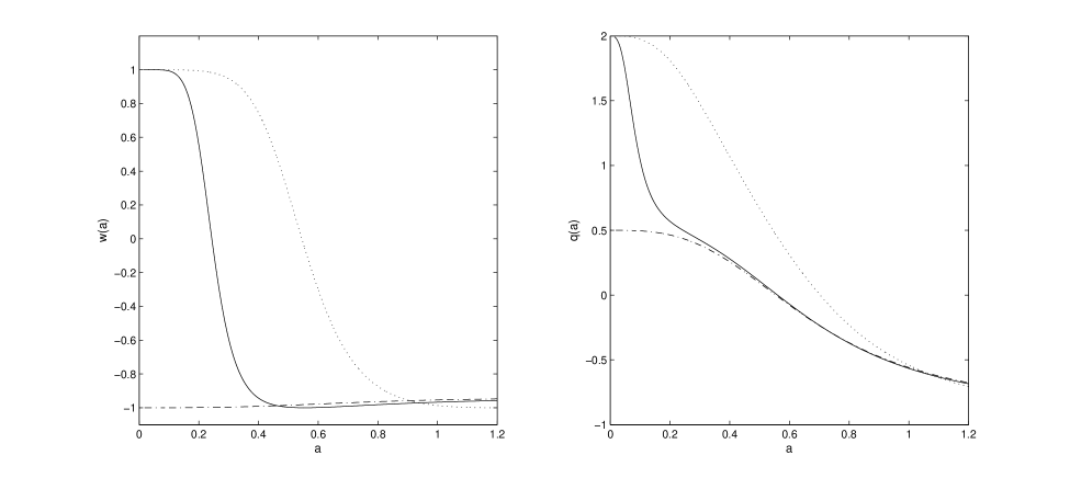
Figure 1: Left: Equation of state $w_{\phi}\left(a\right)$ evolution for scalar field with scale factor (55). Right: Deceleration parameter $q\left(a\right)$ for scale factor (55). We use $\left(\omega_{m0},c_{Q1}\right)=\left(0.12,0.36\right)\times 10^{4}$, $\varepsilon_{\theta}=-1$ ; solid line is for $\theta_{1}=0.01$, the dot line is for $\theta_{1}=0.1$ and the dash dot line is for $\theta_{1}=0.$

V.1.2 UDM: Phantom

For $\varepsilon=-1$ and the potential (41) the Lagrangian of the field equations becomes

$$L\left(a,\phi,\dot{a},\dot{\phi}\right)=-3a\dot{a}^{2}-\frac{1}{2}a^{3}\dot{\phi}^{2}-a^{3}\left(c_{p1}+c_{p2}\cos^{2}\sqrt{\frac{3}{8}}\phi\right)$$ (59)

where the index $P$ denotes the phantom model. Under the coordinate transformation

$$a^{3}=\frac{3}{8}\left(\bar{x}^{2}+\bar{y}^{2}~{}\right),~{}\phi=\sqrt{\frac{8}{3}}\arctan\left(\frac{\bar{y}}{\bar{x}}\right)$$

the field equations are the Hamiltonian constraint

$$-\frac{1}{2}\left(p_{\bar{x}}^{2}+p_{\bar{y}}^{2}\right)+\frac{1}{2}\left(\bar{\omega}_{1}^{2}\bar{x}^{2}+\bar{\omega}_{2}^{2}\bar{y}^{2}\right)=E.$$ (60)

and the Hamilton’s equations of (60). This dynamical system is the 2d unharmonic hyperbolic oscillator where $p_{\bar{x}},p_{\bar{y}}$ are the components of the momentum and $\bar{\omega}_{1}^{2}=\frac{3}{4}\left(c_{p1}+c_{p2}\right)$, $\bar{\omega}_{2}^{2}=\frac{3}{4}c_{p_{1}}.~{}$ The solution of the system is

$$\bar{x}\left(t\right) =\bar{x}_{0}\sinh\left(\bar{\omega}_{1}t+\bar{\theta}_{1}\right)$$

$$\bar{y}\left(t\right) =\bar{y}_{0}\sinh\left(\bar{\omega}_{2}t+\bar{\theta}_{2}\right)$$

for which the Hamiltonian constraint (60) gives $E=-\frac{1}{2}\left(\bar{x}_{0}^{2}\bar{\omega}_{1}^{2}+\bar{y}_{0}^{2}\bar{\omega}_{2}^{2}\right)$. Prior to the singularity we have $a\left(t\rightarrow 0^{+}\right)\rightarrow 0^{+}$ implying $\bar{\theta}_{1}=\bar{\theta}_{2}=0$.

In order to reduce the number of the free parameters we make again the ansazt $c_{p1}=c_{p2}$ and $\bar{x}_{0}=\bar{y}_{0}$. Then from the Hamiltonian constraint we have $\bar{x}_{0}^{2}=\frac{8}{9}\frac{\left|E\right|}{c_{p1}}$ and the analytic solution of the scale factor is

$$a^{3}\left(t\right)=\frac{3}{2}\frac{\omega_{m0}}{\bar{\omega}_{1}^{2}}\left[\sinh^{2}\left(\bar{\omega}_{1}t\right)+\sinh^{2}\left(\frac{\sqrt{2}}{2}\bar{\omega}_{1}t\right)\right].$$ (61)

However, the scalar factor (61) can be written in the following form

$$a\left(t\right)=a_{+}\left(t\right)\sinh^{\frac{2}{3}}\left(\bar{\omega}_{1}t\right)$$ (62)

where

$$a_{+}^{3}\left(t\right)=\frac{3}{2}\frac{\omega_{m0}}{\bar{\omega}_{1}^{2}}\left[1+\left(\frac{\sinh\left(\frac{\sqrt{2}}{2}\bar{\omega}_{1}t\right)}{\sinh\left(\bar{\omega}_{1}t\right)}\right)^{2}\right]$$ (63)

with limit $a_{+}^{3}\left(t\right)|_{\omega_{1}t>>1}=\frac{3}{2}\frac{\omega_{m0}}{\bar{\omega}_{1}^{2}}$, hence in the late time the scale factor (62) is that of the $\Lambda-$cosmology.  Therefore, for the Hubble function holds

$$H\left(t\right)=H_{\Lambda}\left(t\right)+\frac{\dot{a}_{+}\left(t\right)}{a_{+}\left(t\right)}.$$ (64)

V.2 The new hyperbolic model

In the following we use the second integral $I_{2}$ of the hyperbolic potential (46) in order to reduce the order of the dynamical system.

V.2.1 Quintessence, $\varepsilon=1$

For the potential (46) and $\varepsilon=1,$ we apply the coordinate transformation (hyper-parabolic coordinates)

$$a^{3}=\frac{3}{32}\left(u^{2}-v^{2}\right)^{2}~{}\ ,~{}\phi=-\sqrt{\frac{8}{3}}\arctan h\left(\frac{2uv}{u^{2}+v^{2}}\right)$$

and the Lagrangian (36) of the field equations becomes

$$L\left(u,v,\dot{u},\dot{v}\right)=\frac{\left(u^{2}-v^{2}\right)}{2}\left(-\dot{u}^{2}+\dot{v}^{2}\right)-\frac{V_{1}u^{6}-V_{2}v^{6}}{u^{2}-v^{2}}$$ (65)

whereas the Hamiltonian (37) is

$$\left(u^{2}-v^{2}\right)^{-1}\left[\frac{1}{2}\left(-p_{u}^{2}+p_{v}^{2}\right)+\frac{V_{1}}{6}u^{6}-\frac{V_{2}}{6}v^{6}\right]=E$$ (66)

where $p_{u},p_{v}$ are momenta and $V_{1}=\frac{9}{4}\left(c_{Q1}+c_{Q2}\right),$ $V_{2}=\frac{9}{4}\left(c_{Q1}-c_{Q2}\right)$.

Einstein field equations are the Hamiltonian constraint (66) and Hamilton’s equations

$$\left(u^{2}-v^{2}\right)\dot{u}=-p_{u}~{}~{}~{}~{}~{},~{}~{}~{}\left(u^{2}-v^{2}\right)\dot{v}=p_{v}$$

$$\dot{p}_{u}=\frac{2Eu-V_{1}u^{5}}{\left(u^{2}-v^{2}\right)}~{}~{},~{}~{}~{}\ \dot{p}_{v}=-\frac{2Ev-V_{2}v^{5}}{\left(u^{2}-v^{2}\right)}.$$

In order to solve the system of equations we prefer to work with the Hamilton Jacobi equation. Hence from (66) we have

$$\left(u^{2}-v^{2}\right)^{-1}\left[\frac{1}{2}\left(-\left(\frac{\partial S}{\partial u}\right)^{2}+\left(\frac{\partial S}{\partial v}\right)^{2}\right)+\frac{V_{1}}{6}u^{6}-\frac{V_{2}}{6}v^{6}\right]-E\frac{\partial S}{\partial t}=0$$ (67)

where $S=S\left(u,v,t\right)$ is the Hamiltonian and $p_{u}=\frac{\partial S}{\partial u}~{},~{}p_{v}=\frac{\partial S}{\partial v}$.   It is easy to see that (67) is separable, hence the solution is

$$S\left(t,u,v\right)=-\frac{\sqrt{3}}{3}\int\sqrt{V_{1}u^{6}+6\left|E\right|u^{2}+\Phi_{0}}du\pm\frac{\sqrt{3}}{3}\int\sqrt{V_{2}v^{6}+6\left|E\right|v^{2}+\Phi_{0}}dv+t$$

where $\Phi_{0}$ is an integration constant  $\left(\Phi_{0}~{}\varpropto~{}I_{2}\right).$ 

Using the Hamiltonian function we find that the reduced system is

$$\left(u^{2}-v^{2}\right)\dot{u} =\frac{\sqrt{3}}{3}\sqrt{V_{1}u^{6}+6\left|E\right|u^{2}+\Phi_{0}}$$ (68)

$$~{}\left(u^{2}-v^{2}\right)\dot{v} =\pm\frac{\sqrt{3}}{3}\sqrt{V_{2}v^{6}+6\left|E\right|v^{2}+\Phi_{0}}.$$ (69)

From the singularity condition $a\left(t\rightarrow 0\right)=0$ we have that $\left|u\right|_{t\rightarrow 0}=\left|v\right|_{t\rightarrow 0}.$However if in $t\rightarrow 0^{+}$ we consider $u>v>1~{},$ then from (68),(69) we have that $\dot{u}>\dot{v}$, when $V_{1}>V_{2}$ hence in late time hold that $u^{2}>>v^{2},$ then the system (68), (69) becomes

$$\dot{u}=\mu_{1}u~{},~{}\dot{v}=\pm\mu_{2}\frac{v^{3}}{u^{2}}$$

where $\mu_{1,2}=\frac{\sqrt{3}}{3}\sqrt{V_{1,2}}$; hence the solution of the scale factor is

$$a^{\frac{3}{2}}\left(t\right)=a_{1}e^{2\mu_{1}t}\mp\frac{a_{1}^{2}\mu_{1}^{2}}{\mu_{2}e^{-2\mu_{1}t}+a_{1}^{2}a_{2}\mu_{1}}$$ (70)

when $a_{2}=0$ the scale factor (70) becomes

$$a^{\frac{3}{2}}\left(t\right)=\left(a_{1}\mp\frac{a_{1}^{2}\mu_{1}^{2}}{\mu_{2}}\right)e^{2\mu_{1}t}$$ (71)

which is the deSitter solution.

In Fig. 2   we give the evolution of the equation of state parameter of the scalar field and the evolution of the deceleration parameter of the model with Lagrangian (65) where in (69) we considered the minus. We observe that for the equation of state parameter $w_{\phi}$ holds $w_{\phi}\left(a\rightarrow 1\right)=-1$ provided that the integration constant $\Phi_{0}$ satisfies the condition $\log\Phi_{0}\leq 1$.

Figure 2: In the left fig. we give the equation of state $w_{\phi}\left(a\right)$ evolution of the scalar field with Lagrangian (65) and in the right fig. we give the deceleration parameter $q\left(a\right)$ of the scale factor with Lagrangian (65) where in (69) we considered the sing minus. For the numeric solution we use $\left(u,v\right)_{t\rightarrow 0}=\left(0.01,0.0998\right),~{}$ $\left(\rho_{m0},c_{1},c_{2}\right)=\left(0.33,1,0.8\right)\times 10^{4};$ solid line is for $\Phi_{0}=0$, the dot line is for $\Phi_{0}=10^{3}$ and the dash dot line is for $\Phi_{0}=10^{4}.$

Exact solution

The dynamical system (68), (69) is a non linear 2d system of first order ODEs. In order to solve this system analytically we consider the ”conformal” transformation $\ dt=\sqrt{3}\left(u^{2}-v^{2}\right)d\tau~{},~{}$i.e. $dt\cong a^{\frac{3}{2}}d\tau$ which transforms the dynamical system to

$$u^{\prime} =\sqrt{V_{1}u^{6}+6\left|E\right|u^{2}+\Phi_{0}}$$ (72)

$$v^{\prime} =\sqrt{V_{2}v^{6}+6\left|E\right|v^{2}+\Phi_{0}}$$ (73)

where $u^{\prime}=\frac{du}{d\tau}$.  From (72),(73) follows

$$\int\frac{du}{\sqrt{V_{1}u^{6}+6\left|E\right|u^{2}+\Phi_{0}}} =\int d\tau~{}~{}~{}$$ (74)

$$~{}\int\frac{dv}{\sqrt{V_{2}v^{6}+6\left|E\right|v^{2}+\Phi_{0}}} =\int d\tau.$$ (75)

The solution of (74), (75) can be written in terms of elliptic functions.  In order to simplify the integrals (74), (75)  and obtain an explicit solution we select special values for the constants. For $\Phi_{0}=0$ and $E=0$ the solution of the system (74),(75) gives the deSitter universe (71).

However when $\Phi_{0}=0$ and $E\neq 0$ the solution of the system (74),(75) is

$$u\left(\tau\right) =\frac{2\exp\left(C_{1}\left(\tau-\tau_{0}\right)\right)}{\sqrt{\exp\left(\pm 4\sqrt{6\left|E\right|}\left(\tau-\tau_{0}\right)\right)-4C_{1}^{2}}}$$

$$v\left(\tau\right) =\frac{2\exp\left(C_{2}\left(\tau-\tau_{0}\right)\right)}{\sqrt{\exp\left(4\sqrt{6\left|E\right|}\left(\tau-\tau_{0}\right)\right)-4C_{2}^{2}}}$$

where $C_{1,2}=\varepsilon_{C}\left(\frac{6\left|E\right|}{V_{1,2}}\right)^{\frac{1}{2}}$ , $\varepsilon_{C}=\pm 1~{}$and from the relation $dt=\sqrt{3}\left(u^{2}-v^{2}\right)d\tau$ we have

$$t-t_{0}=\sqrt{3}\left[\ln\left(\frac{2C_{1}e^{2C_{1}\tau_{0}}-e^{2C_{1}\tau}}{2C_{1}e^{2C_{1}\tau_{0}}+e^{2C_{1}\tau}}\right)+\ln\left(\frac{2C_{2}e^{2C_{2}\tau_{0}}+e^{2C_{2}\tau}}{2C_{2}e^{2C_{2}\tau_{0}}-e^{2C_{2}\tau}}\right)\right].$$

V.2.2 Phantom, $\varepsilon=-1$

In the case of phantom scalar field, i.e. $\varepsilon=-1$,   in parabolic coordinates

$$a^{3}=\frac{3}{32}\left(w^{2}+z^{2}\right)^{2}~{}\ ,~{}\phi=\sqrt{\frac{8}{3}}\arctan\left(\frac{2wz}{w^{2}-z^{2}}\right)$$ (76)

the Lagrangian (36) of the field equations becomes

$$L\left(w,z,\dot{w},\dot{z}\right)=-\frac{\left(w^{2}+z^{2}\right)}{2}\left(\dot{w}^{2}+\dot{z}^{2}\right)+\frac{V_{1}w^{6}+V_{2}z^{6}}{u^{2}+v^{2}}.$$

The field equations are the Hamiltonian

$$-\frac{1}{\left(w^{2}+z^{2}\right)}\left[\frac{1}{2}\left(p_{w}^{2}+p_{z}^{2}\right)-\frac{\bar{V}_{1}}{6}w^{6}-\frac{\bar{V}_{2}}{6}z^{6}\right]=E$$ (77)

and Hamilton’s equations of (77), where $p_{w},p_{z}$ are the momenta and $\bar{V}_{1}=\frac{9}{4}\left(c_{p1}+c_{p2}\right),$ $\bar{V}_{2}=\frac{9}{4}\left(c_{p2}-c_{p1}\right).$

Working as previously we find that the solution of the Hamilton Jacobi equation is

$$S\left(t,w,z\right)=-\frac{\sqrt{3}}{3}\int\sqrt{\bar{V}_{1}w^{6}+6\left|E\right|w^{2}+\Phi_{0}}dw\pm\frac{\sqrt{3}}{3}\int\sqrt{\bar{V}_{2}z^{6}+6\left|E\right|z^{2}-\Phi_{0}^{\prime}}dz-t.$$

Therefore the reduced dynamical system is

$$\left(w^{2}+z^{2}\right)\dot{w} =\frac{\sqrt{3}}{3}\sqrt{\bar{V}_{1}w^{6}+6\left|E\right|w^{2}+\Phi_{0}^{\prime}}$$ (78)

$$\left(w^{2}+z^{2}\right)\dot{z} =\pm\frac{\sqrt{3}}{3}\sqrt{\bar{V}_{2}z^{6}+6\left|E\right|z^{2}-\Phi_{0}^{\prime}}$$ (79)

The dynamical system (78), (79) is a two dimensional nonlinear system. In order to simplify it we may apply the conformal transformation $dt=\sqrt{3}\left(w^{2}+z^{2}\right)d\tau,~{}$i.e. $dt\cong a^{\frac{3}{2}}d\tau,$ as we did in section V.2.1. Furthermore, from the singularity condition $a\left(t\rightarrow 0^{+}\right)\rightarrow 0^{+}$, we have $\left(w,z\right)_{t\rightarrow 0}=0;$ hence,  in order to avoid complex solutions of the system (78), (79) we set $\Phi_{0}^{\prime}=0$.

VI Observational constraints

In this section, we test the viability of the cosmological model in the late times (well inside the matter era) resulting for the scalar field potentials we have determined, by performing a joint likelihood analysis using the SNIa, BAO and the $H\left(z\right)$ data. The likelihood function is

$$\mathcal{L}\left(\mathbf{p}\right)\mathcal{=L}_{SNIa}\mathcal{\times L}_{BAO}\mathcal{\times L}_{H\left(z\right)}$$ (80)

where $\mathbf{p}$ is the statistical vector that contains the free parameters and $\mathcal{L}_{A}\varpropto e^{-\chi_{A}^{2}/2}~{}$; that is, $\chi^{2}=\chi_{SNIa}^{2}+\chi_{BAO}^{2}+\chi_{H\left(z\right)}^{2}$.

For the Type Ia supernova data we use the Union 2.1 set which provides us with 580 SNIa distance modulus at observed redshift Suzuki . The chi-square is given by the expression

$$\chi_{SNIa}^{2}=\sum\limits_{i=1}^{N_{SNIa}}\left(\frac{\mu_{obs}\left(z_{i}\right)-\mu_{th}\left(z_{i};\mathbf{p}\right)}{\sigma_{i}}\right)^{2}$$ (81)

where $N_{SNIa}=580$, $z_{i}$ is the observed redshift $z_{i}\in$ $\left[0.015,1.414\right]$, $\mu$ is the distance modulus $\mu=m-M=5\log D_{L}+25$ and $D_{L}$ is the luminosity distance.

The chi-square for the Hubble parameter constraint data is

$$\chi_{H\left(z\right)}^{2}=\sum\limits_{i=1}^{N_{H(z)}}\left(\frac{H_{obs}\left(z_{i}\right)-H_{th}\left(z_{i};\mathbf{p}\right)}{\sigma_{i}}\right)^{2}$$ (82)

where $N_{H(z)}=21$, $H_{th}\left(z_{i};\mathbf{p}\right)$ is the theoretical Hubble parameter and $H_{obs}$ are the 21 observed Hubble parameters at the observed redshift $z_{i}$ simon ; stern ; Gaz ; mar (see Table 1 of Farooq ).

Furthermore we use the 6dF, the SDSS and WiggleZ BAO data Percival ; BlakeC for which the corresponding chi-square is

$$\chi_{BAO}^{2}=\sum\limits_{i=1}^{N_{BAO}}\left(\sum\limits_{j=1}^{N_{BAO}}\left[d_{obs}\left(z_{i}\right)-d_{th}\left(z_{i};\mathbf{p}\right)\right]C_{ij}^{-1}\left[d_{obs}\left(z_{j}\right)-d_{th}\left(z_{j};\mathbf{p}\right)\right]\right)$$ (83)

where $N_{BAO}=6$, $C_{ij}^{-1}$ is the inverse of the covariant matrix in terms of $d_{z}~{}\$BasilNess , and the parameter $d_{z}$ follows from the relation $d_{z}=\frac{l_{BAO}}{D_{V}\left(z\right)}$; $~{}l_{BAO}\left(z_{drag}\right)$ is the BAO scale at the drag redshift and $D_{V}\left(z\right)$ is the volume distance BlakeC .

Without losing the generality in the case of the quintessence UDM model we set $\theta_{1}\rightarrow 0$. Therefore, the UDM statistical vector $\mathbf{p~{}}$is of dimension two $\left(\dim\mathbf{p=2}\right);$ that is, $\mathbf{p=}\left(\omega_{m0},c_{\left(Q,p\right)1}\right),$ recall that $\omega_{m0}=\Omega_{m0}H_{0}^{2}$, and $\rho_{m0}=3\omega_{m0}=\left|E\right|.$ In order to constraint the new hyperbolic scalar field with potential (46) with the data, we have to define six free parameters, that is, $c_{\left(Q,p\right)1},c_{\left(Q,p\right)2},\omega_{m0}$, $\Phi_{0}/\Phi_{0}^{{}^{\prime}}$ and the initial conditions$~{}\left(u,v\right)/\left(w,z\right)$. In order to reduce the number of the free parameters we make the ansatz $c_{\left(Q,p\right)2}=0.8c_{\left(Q,p\right)1}.$ Furthermore from the singularity condition $a\left(t\rightarrow 0^{+}\right)\rightarrow 0^{+}$ we select the initial conditions $\left(u,v\right)_{t\rightarrow 0^{+}}=\left(0.1,0.0998\right),~{}\left(w,z\right)_{{}_{t\rightarrow 0^{+}}}=\left(10^{-3},10^{-4}\right)~{}$where in (69) we considered the sign minus $"-"~{}$and in (79) the sign plus $"+"$. Finally we assume the integration constants $\Phi_{0}/\Phi_{0}^{{}^{\prime}}~{}$to vanish .

Lastly, since $N/n_{fit}>40$ we will use, the relevant to our case, corrected Akaike information criterion Akaike1974 , defined, for the case of Gaussian errors, as:

$$\mathrm{AIC}=\chi_{min}^{2}+2n_{fit}$$ (84)

where $N=N_{SNIa}+N_{H(z)}+N_{BAO}=607$ and $n_{fit}$ is the number of free parameters. A smaller value of AIC indicates a better model-data fit (for the scalar field models $n_{fit}=2$ and for the $\Lambda$CDM we have $n_{fit}=2$). However, small differences in AIC are not necessarily significant and therefore, in order to assess, the effectiveness of the different models in reproducing the data, one has to investigate the model pair difference $\Delta$AIC$=\mathrm{AIC}_{y}-\mathrm{AIC}_{x}$. The higher the value of $|\Delta\mathrm{AIC}|$, the higher the evidence against the model with higher value of $\mathrm{AIC}$, with a difference $|\Delta$AIC$|\raise-3.0pt\hbox{\hbox to0.0pt{\hbox{$\sim$}\hss}\raise 4.0pt\hbox{$>$}\ }2$ indicating a positive such evidence and $|\Delta$AIC$|\raise-3.0pt\hbox{\hbox to0.0pt{\hbox{$\sim$}\hss}\raise 4.0pt\hbox{$>$}\ }6$ indicating a strong such evidence, while a value $\raise-3.0pt\hbox{\hbox to0.0pt{\hbox{$\sim$}\hss}\raise 4.0pt\hbox{$<$}\ }2$ indicates consistency among the two comparison models.

The scalar field with potential (41) has been compared with the cosmological data in BasilLukes for the quintessence field and in capPhantom for the phantom field. In contrast to BasilLukes in our solution we include the dark matter component in the field equations. Furthermore in capPhantom the authors examine the case where $\bar{c}_{p1}=0~{}$and$~{}\bar{c}_{p2}\neq 0$.

Table 1: Best fit values and cosmological parameters for the SNIa+BAO and SNIa+BAO+H(z) tests for the $\Lambda$-cosmology and for the Scalar fields dark energy models which admit dynamical symmetries. The final three column present the goodness-of-fit statistics $\chi^{2}_{min}$ parameter

$\Lambda$CDM	$\Omega_{m0}$	$H_{0}$	$w_{\Lambda}~{}$(fixed)	$\omega_{m0}\times 10^{-4}$	$\chi_{min}^{2}$
SNIa+BAO	$0.29_{-0.032}^{+0.016}$	$68.4_{-1.40}^{+0.70}$	$-1.000$	$0.14$	$560.32$
SNIa+BAO+H(z)	$0.29_{-0.020}^{+0.016}$	$68.4_{-0.10}^{+2.70}$	$-1.000$	$0.14$	$574.77$
Scalar Field (41)	$\Omega_{m0}$	$H_{0}$	$w_{\phi 0}$	$\left(\omega_{m0},c_{\left(Q,p\right)1}\right)\times 10^{-4}$	$\chi_{min}^{2}$
Quintessence, $\varepsilon=1$
SNIa+BAO	$0.25$	$68.1$	$-0.965$	$\left(0.12_{-0.019}^{+0.031},0.39_{-0.052}^{+0.020}\right)$	$563.48$
SNIa+BAO+H(z)	$0.28$	$69.8$	$-0.968$	$\left(0.13_{-0.009}^{+0.015},0.39_{-0.028}^{+0.016}\right)$	$577.82$
Phantom, $\varepsilon=-1$
SNIa+BAO	$0.29$	$67.9$	$-1.017$	$\left(0.13_{-0.021}^{+0.020},0.58_{-0.048}^{+0.088}\right)$	$562.93$
SNIa+BAO+H(z)	$0.30$	$69.6$	$-1.016$	$\left(0.15_{-0.013}^{+0.008},0.60_{-0.012}^{+0.060}\right)$	$576.59$
Scalar Field (46)	$\Omega_{m0}$	$H_{0}$	$w_{\phi 0}$	$\left(\omega_{m0},c_{\left(Q,p\right)1}\right)\times 10^{-4}$	$\chi_{min}^{2}$
Quintessence, $\varepsilon=1$
SNIa+BAO	$0.27$	$67.9$	$-1.000$	$\left(0.12_{-0.014}^{+0.026},0.14_{-0.010}^{+0.015}\right)$	$562.84$
SNIa+BAO+H(z)	$0.28$	$69.7$	$-1.000$	$\left(0.14_{-0.005}^{+0.015},0.15_{-0.010}^{+0.009}\right)$	$576.76$
Phantom, $\varepsilon=-1$
SNIa+BAO	$0.27$	$68.3$	$-1.044$	$\left(0.13_{-0.017}^{+0.023},0.15_{-0.012}^{+0.014}\right)$	$562.75$
SNIa+BAO+H(z)	$0.29$	$69.6$	$-1.048$	$\left(0.14_{-0.002}^{+0.009},0.15_{-0.013}^{+0.006}\right)$	$576.65$

In table 1 we give a numerical summary of the current statistical analysis  and the scalar field models with potentials (41), (46). For the $\Lambda$-cosmology we find the minimum total chi-square $\chi_{min}^{2}=574.77$ ($\mathrm{dof}=606$) with best fit values $\left(\Omega_{m0},H_{0}\right)_{\Lambda}=\left(0.29,68.4\right)$. For the scalar field model (41) we find for the quintessence field $\min_{Q1}\chi_{min}^{2}=577.82$ ($\mathrm{dof}=605$) and for the best fit values of the parameters $\omega_{m0},c_{Q1}$ we have the cosmological parameters $\left(\Omega_{m0},H_{0},w_{\phi 0}\right)_{Q1}=\left(0.28,69.8,-0.968\right)$ whereas for the phantom field we have $\chi_{min}^{2}=576.59$ and $\left(\Omega_{m0},H_{0},w_{\phi 0}\right)_{P1}=\left(0.30,69.6,-1.016\right).$

Similarly for the potential (46) we find for the quintessence field $\chi_{min}^{2}=576.76$,  $\left(\Omega_{m0},H_{0},w_{\phi 0}\right)_{Q2}=\left(0.28,69.7,-1.000\right)$ and for the phantom field $\chi_{min}^{2}=576.65$,  $\left(\Omega_{m0},H_{0},w_{\phi 0}\right)_{P2}=\left(0.29,69.6,-1.048\right).$

As it is expected the value of AIC_Λ($\simeq 578.77$) is smaller than the corresponding values of the scalar field models AIC_scalar($580.59-581.82$) which indicates that the $\Lambda$CDM model appears to fit better than the scalar fields models the expansion data. However, the differential value $|\Delta\mathrm{AIC}|$=$|\mathrm{AIC}_{\Lambda}-\mathrm{AIC}_{scalar}|$ is actually $\leq 2$ which indicates that the cosmological data are perfectly consistent with the current scalar field models in a way comparable to the concordance model.

In order to give the reader the opportunity to appreciate our observational constraints, in fig. 3 and 4 we provide the likelihood contours for the best fit parameters $\left(\omega_{m0},c_{\left(Q,p\right)1}\right)$ of the scalar fields with potentials (41) and (46).

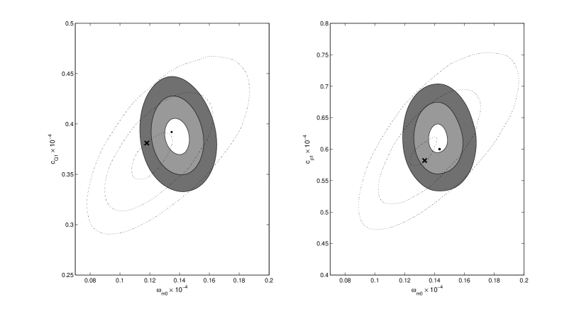
Figure 3: Likelihood contours of $1\sigma~{}\left(\Delta\chi^{2}=2.3\right),2\sigma~{}\left(\Delta\chi^{2}=6.18\right)$ and $3\sigma~{}\left(\Delta\chi^{2}=11.83\right)$ in the plane $\left(\omega_{m0},c_{\left(Q,p\right)1}\right)$ for the scalar field with potential (41). Left figure is for the Quintessence field whereas right figure is for the Phantom field. The filled areas are for the SnIa+BAO+H(z) test, the best fit values are marked with a dot; the dot lines are for the SnIa+BAO test and the best fit values are marked with $\times$.  

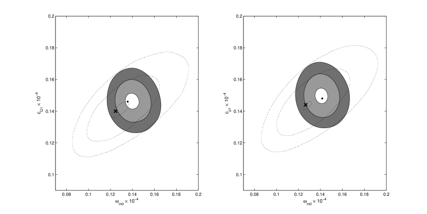
Figure 4: Likelihood contours of $1\sigma~{}\left(\Delta\chi^{2}=2.3\right),2\sigma~{}\left(\Delta\chi^{2}=6.18\right)$ and $3\sigma~{}\left(\Delta\chi^{2}=11.83\right)$ in the plane $\left(\omega_{m0},c_{\left(Q,p\right)1}\right)$ for the scalar field with potential (46). Left figure is for the Quintessence field whereas right figure is for the Phantom field. The filled areas are for the SnIa+BAO+H(z) test, the best fit values are marked with a dot; the dot lines are for the SnIa+BAO test and the best fit values are marked with $\times$.  

VII Conclusion

In this work we have applied the dynamical Noether symmetry approach as a geometric rule to select the potential of the scalar field in the scalar field cosmology. We have found two potentials with this property and have used the resulting Noether integrals to integrate the corresponding field equations. The first potential is the well known UDM model whereas the second potential is new. In both cases we have found the analytic solution of the field equations both in the quintessence and in the phantom case. The solution for the new potential is expressed in terms of elliptic functions and contains a number of free parameters.  In order to find an explicit analytic solution we consider certain simplifications which are compatible with the physical assumptions. Furthermore we test the solutions we have found against the observed cosmological constraints that is, the SNIa, BAO and the $H\left(z\right)$ data. We find that the cosmological parameters for the scalar field models which admit dynamical symmetries are similar with those of the $\Lambda$-cosmology

Besides the actual value of the new solution the approach shows that the use of careful geometric requirements/ assumptions can help in two directions, namely a.) to produce new results which is impossible to be found by ordinary physical reasoning and b) to lead to models with a large number of free parameters which provide adequate freedom of adjustment; in the sense that the values of the constants are fixed in accordance with the observed data, therefore leading to viable/ sound cosmological models.

Appendix A Classification of scalar field potentials which admit dynamical symmetries

In this appendix we give the complete classification of the potentials for which the Lagrangian (39) admits contact Noether symmetries. We have the following results.

• If the scalar field potential is

  $$V\left(\theta\right)=c_{1}\left(1-3\sinh^{2}\theta\right)+c_{2}\left(3\sinh\theta-\sinh^{3}\theta\right)$$ (85)

  Lagrangian (39) admits the additional dynamical symmetry

  $$X=-r^{2}\cosh\theta~{}\dot{\theta}\partial_{r}+\left(\cosh\theta~{}\dot{r}+2r\sinh\theta~{}\dot{\theta}\right)\partial_{\theta}$$ (86)

  with corresponding Noether Integral

  $$\bar{I}_{2}=\left(\cosh\theta~{}\dot{r}+r\sinh\theta~{}\dot{\theta}\right)r^{2}\dot{\theta}-r^{3}\cosh^{2}\theta\left(2c_{1}\sinh\theta-c_{2}\left(1-\sinh^{2}\theta\right)\right).$$ (87)

  This potential is equivalent to potential (46) under the transformation $\theta=\bar{\theta}+i\frac{\pi}{2}.$

• If the scalar field potential is

  $$V\left(\theta\right)=c_{1}+c_{2}e^{2\theta}$$ (88)

  Lagrangian (39) admits the dynamical symmetry

  $$X=-e^{2\theta}\left(\dot{r}+r\dot{\theta}\right)\partial_{r}+\frac{e^{2\theta}}{r}\left(\dot{r}+r\dot{\theta}\right)\partial_{\theta}$$ (89)

  with corresponding Noether Integral

  $$I_{3}=e^{2\theta}\left(\left(\dot{r}+r\dot{\theta}\right)^{2}-2r^{2}c_{1}\right)$$ (90)

  When $c_{1}=0$ the dynamical system admits the additional dynamical symmetry

  $$X_{3}=-r^{2}e^{\theta}\dot{\theta}\partial_{r}+e^{\theta}\left(\dot{r}+2r\dot{\theta}\right)\partial_{\theta}$$ (91)

  with corresponding Noether Integral

  $$\bar{I}_{3}=r^{2}e^{\theta}\left(\dot{r}\dot{\theta}+r\dot{\theta}^{2}\right)+\frac{2}{3}c_{2}r^{3}e^{3\theta}.$$ (92)

• In the case where the potential is

  $$V\left(\theta\right)=c_{1}e^{2\theta}+c_{2}e^{3\theta}$$ (93)

  Lagrangian (39) admits the dynamical symmetry (91) with corresponding Noether Integral

  $$I_{3}=r^{2}e^{\theta}\left(\dot{r}\dot{\theta}+r\dot{\theta}^{2}\right)+r^{3}e^{3\theta}\left(\frac{2}{3}c_{1}+c_{2}e^{\theta}\right).$$ (94)

  Note that the potential (93) can be seen in the context of the early dark energy potential Bar00 .

In order to complete our analysis in appendix B we apply the integral (94) in order to reduce the order of the field equations with potential (93).

Appendix B Reduction of order for the early dark energy potential with $\left(\lambda_{1},\lambda_{2}\right)=\left(2,3\right).$

In this appendix we reduce the field equations of the model with potential (93). In this case Lagrangian (36) becomes

$$L\left(a,\phi,\dot{a},\dot{\phi}\right)=-3a\dot{a}^{2}+\frac{1}{2}a^{3}\dot{\phi}^{2}-a^{3}\left(c_{1}e^{\frac{\sqrt{6}}{2}\phi}+c_{2}e^{\frac{3\sqrt{6}}{4}\phi}\right)$$ (95)

We consider the coordinate transformation

$$a^{3}=\frac{3}{8}\xi^{2}\eta~{},~{}\phi=\sqrt{\frac{8}{3}}\ln\left(\frac{\sqrt{\eta}}{\xi}\right)$$

by which the Lagrangian (95) becomes

$$L\left(\xi,\eta,\dot{\xi},\dot{\eta}\right)=-\xi\dot{\eta}\dot{\xi}-\bar{c}_{1}\eta^{2}-\bar{c}_{2}\frac{\eta^{\frac{5}{2}}}{\xi}$$

where $\bar{c}_{1,2}=\frac{3}{8}c_{1,2}$. The Hamiltonian in normal coordinates is

$$E=-\frac{p_{\xi}p_{\eta}}{\xi}+\bar{c}_{1}\eta^{2}+\bar{c}_{2}\frac{\eta^{\frac{5}{2}}}{\xi}$$ (96)

The field equations are the Hamiltonian constraint (96) and Hamilton’s equations

$$\xi\dot{\eta}=-p_{\xi}~{}~{},~{}~{}\xi\dot{\xi}=-p_{\eta}$$

$$\dot{p}_{\xi}=\frac{c_{2}\eta^{\frac{5}{2}}-p_{\xi}p_{\eta}}{\xi^{2}}~{}~{},~{}~{}\dot{p}_{\eta}=-\left(2\bar{c}_{1}\eta+\frac{5}{2}\bar{c}_{2}\frac{\eta^{\frac{3}{2}}}{\xi}\right).$$

We note that (96) is in the form of equations (16) and (18) of Daskal (where $F\left(\eta\right)=1,~{}G\left(\eta\right)=0,~{}f\left(\eta\right)=\bar{c}_{1}\eta^{2}$ and $g\left(\eta\right)=\bar{c}_{2}\eta^{\frac{5}{2}}$). The solution of the Hamilton Jacobi equation

$$-\frac{1}{\xi}\left(\frac{\partial S}{\partial\xi}\right)\left(\frac{\partial S}{\partial\eta}\right)+\bar{c}_{1}\eta^{2}+\bar{c}_{2}\frac{\eta^{\frac{5}{2}}}{\xi}-E\frac{\partial S}{\partial t}=0$$

is

$$S\left(t,\xi,\eta\right)=-\frac{\xi}{3}\sqrt{6\bar{c}_{1}\eta^{3}+18\left|E\right|~{}\eta+\Phi_{0}}-\int\frac{3\bar{c}_{2}\eta^{\frac{5}{2}}}{\sqrt{6\bar{c}_{1}\eta^{3}+18\left|E\right|~{}\eta+\bar{\Phi}_{0}}}d\eta-t.$$

where $\bar{\Phi}_{0}\propto I_{3}$.

Therefore the reduced Hamilton’s equations are

$$\xi\dot{\eta} =\frac{1}{3}\sqrt{6\bar{c}_{1}\eta^{3}+18\left|E\right|\eta+\bar{\Phi}_{0}}$$ (97)

$$~{}~{}\xi\dot{\xi} =\frac{3\left(\left(\bar{c}_{1}\eta^{2}+\left|E\right|\right)\xi+\bar{c}_{2}\eta^{\frac{5}{2}}\right)}{\sqrt{6\bar{c}_{1}\eta^{3}+18\left|E\right|~{}\eta+\bar{\Phi}_{0}}.}$$ (98)

References

- (1) M. Tegmark et al., Astrophys. J. 606, 702 (2004)
- (2) D. N. Spergel et al., Astrophys. J. Suplem. 170, 377 (2007)
- (3) T. M. Davis et al., Astrophys. J. 666, 716 (2007)
- (4) M. Kowalski et al., Astrophys. J. 686, 749(2008)
- (5) M. Hicken et al., Astroplys. J. 700, 1097 (2009)
- (6) E. Komatsu et al., Astrophys. J. Suplem. 180, 330 (2009); G. Hinshaw et al., Astrophys. J. Suplem. 180, 225 (2009)
- (7) J. A. S. Lima and J. S. Alcaniz, Mon. Not. Roy. Astron. Soc. 317, 893 (2000); J. F. Jesus and J. V. Cunha, Astrophys. J. Lett. 690, L85 (2009)
- (8) S. Basilakos and M. Plionis, Astrophys. J. Lett. 714, 185 (2010)
- (9) E. Komatsu et al., Astrophys. J. Suplem. 192, 18 (2011)
- (10) P.A.R Ade, et al., (Planck Collaboration), (2013), [arXiv:1303.5076]
- (11) E. J. Copeland, M. Sami and S. Tsujikawa, Intern. Journal of Modern Physics D, 15, 1753,(2006); L. Amendola and S. Tsujikawa, Dark Energy Theory and Observations, Cambridge University Press, Cambridge UK, (2010); R. R. Caldwell and M. Kamionkowski, Ann.Rev.Nucl.Part.Sci., 59, 397 (2009); I. Sawicki and W. Hu, Phys. Rev. D., 75, 127502 (2007)
- (12) S. Weinberg, Rev. Mod. Phys. 61 1, (1989)
- (13) P.J. Peebles and B. Ratra, Rev. Mod. Phys. 75 559 (2003)
- (14) T. Padmanabhan, Phys. Rept. 380 235, (2003)
- (15) P.J Steinhardt, Phil. Trans. R. Soc. Lond. A. 361 2497 (2003)
- (16) C. A. Egan and C. H. Lineweaver, Phys. Rev. D. 78 3528 (2008)
- (17) B. Ratra and P. J. E. Peebles, Phys. Rev. D 37 3406 (1988)
- (18) M. Ozer and O. Taha, Nucl. Phys. B 287 776 (1987)
- (19) W. Chen and Y.S. Wu, Phys. Rev. D 41 695 (1990)
- (20) J. C. Carvalho, J. A. S. Lima and I. Waga, Phys. Rev. D 46, 2404 (1992)
- (21) J. A. S. Lima and J. M. F. Maia, Phys. Rev D 49 5597 (1994)
- (22) S. Basilakos, M. Plionis and S. Solà, Phys. Rev. D. 80 083511 (2009)
- (23) R. R. Caldwell, R. Dave, and P.J. Steinhardt, Phys. Rev. Lett., 80 1582 (1998)
- (24) A. Kamenshchik, U. Moschella, and V. Pasquier, Phys. Lett. B. 511 265 (2001)
- (25) R. R. Caldwell, Phys. Rev. Lett. B., 545 23 (2002).
- (26) M. C. Bento, O. Bertolami, and A.A. Sen, Phys. Rev. D., 70 083519 (2004)
- (27) L. P. Chimento, and A. Feinstein, Mod. Phys. Lett. A, 19 761 (2004)
- (28) E. V. Linder, Phys. Rev. D. 70, 023511 (2004)
- (29) J. A. S. Lima, F. E. Silva and R. C. Santos, Class. Quant. Grav. 25 205006 (2008)
- (30) L. Samushia, B. Ratra, Astrophys. J. 650, L5, (2006); Astrophys. J. 680 L1 (2008)
- (31) J.Q. Xia, H. Li, G.B. Zhao and X. Zhang, Phys. Rev. D 78 083524 (2008)
- (32) J. Simon, L. Verde, R. Jiménez, Phys. Rev. D 71 123001 (2005)
- (33) S. Basilakos, J. C. Sanchez, L. Perivolaropoulos, Phys. Rev. D. 80 043530 (2009)
- (34) A. D. Dolgov, in: The very Early Universe, edited by G. Gibbons, S.W. Hawking, and S. T. Tiklos, Cambridge University Press, Cambridge, England (1982)
- (35) P. Brax and J. Martin, Phys. Lett. B 468 10 (1999)
- (36) J. L. Sievers et al., Astrophys. J. 591 599 (2003)
- (37) D. Bertacca, S. Matarrese and M. Pietroni Mod. Phys. Lett. A 22 2893 (2007)
- (38) J. A. Frieman, C. T. Hill, A Stwebbins, and I. Waga, Phys. Rev. Lett. 75 2077 (1995)
- (39) P. J. Steinhardt, L. Wang, and I. Zlatev, Phys. Rev. D 59 123504 (1999)
- (40) T. Barreiro, E. Copeland, and N. J. Nunes, Phys. Rev. D 61, 127301 (2000)
- (41) V. Sahni and L.M. Wang, Phys. Rev. D 62 103517 (2000)
- (42) R. de Ritis, et al. Phys. Rev. D 42 1091 (1990)
- (43) S. Capozziello, R de Ritis, C. Rubano, and, P. Scudellaro, Riv. Nuovo Cim., 19, 1, (1996); M. Szydlowski et al., Gen. Rel. Grav., 38, 795, (2006); S. Capozziello, S. Nesseris, and L. Perivolaropoulos, JCAP, 0712, 009, (2007); Yi Zhang, Yun-gui Gong and Zong-Hong Zhu, Phys. Lett. B., bf 688, 13, (2010); S. Capozziello and De Felice, JCAP, 0808, 016, (2008); P.A. Terzis, N. Dimakis and T. Christodoulakis arXiv:1410.0802
- (44) M. Tsamparlis and A. Paliathanasis, Gen. Relativ. Gravit. 43 1861 (2011)
- (45) A. V. Aminova, Tensor N.S., 62 65 (2000)
- (46) G.E. Prince and M. Crampin, Gen Relativ. Gravit. 16 921 (1984)
- (47) A. Paliathanasis and M. Tsamparlis, J. Geometry and Physics 62 2443 (2012)
- (48) V. Gorini, A. Kamenshchik, U. Moschella, V. Pasquier, Phys. Rev. D, 69, 123512, (2004)
- (49) V. Gorini, A. Kamenshchik, U. Moschella, V. Pasquier, A. Starobinsky, Phys. Rev. D, 72, 103518, (2005)
- (50) S. Basilakos, M. Tsamparlis and A. Paliathanasis, Phys. Rev. D. 83 103512 (2011)
- (51) S. Capozziello, E. Piedipalumbo, C. Rubano and P. Scudellaro, Phys. Rev. D. 80 104030 (2009)
- (52) B. Vakili, F. Khazaie, Class. Quant. Grav. 29 035015 (2012)
- (53) S. Cotsakis, P.G.L. Leach and H. Pantazi, Grav. Cosm. 4 314 (1998)
- (54) A. Paliathanasis and M. Tsamparlis, Phys. Rev. D. 90 (2014) 043529
- (55) A. Paliathanasis, M. Tsamparlis and S. Basilakos, Phys. Rev. D. 84 123514 (2011)
- (56) H. Wei, X.J. Guo and L.F. Wang, Phys. Lett. B. 707 298 (2012)
- (57) S. Capozziello, M. De Laurentis and S.D. Odintsov, Eur. Phys. J. C 72 2068 (2012)
- (58) R.C. de Souza, R. Andre and G. M. Kremer Phys. Rev. D 87 08351 (2013)
- (59) Y. Kucukakca, Eur. Phys. J. C 73 2327 (2013)
- (60) S. Capozziello, A. Stabile, and A. Troisi, Class. Quant. Grav. 24 2153 (2007)
- (61) Vakili B., Phys. Lett. B. 669 (2008) 206
- (62) H. Dong, J. Wang and X. Meng, Eur. Phys. J. C 73 2543 (2013)
- (63) S. Basilakos, S. Capozziello, M. De Laurentis, A. Paliathanasis and M. Tsamparlis, Phys. Rev. D. 88 103526 (2013)
- (64) A. Paliathanasis, S. Basilakos, E.N. Saridakis, S. Capozziello, K. Atazadeh, F. Darabi and M. Tsamparlis, Phys. Rev. D. 89 104042 (2014)
- (65) A. Paliathanasis, M. Tsamparlis, S. Basilakos and S. Capozziello, Phys. Rev. D. 89 063532 (2014)
- (66) H. Stephani, Differential Equations: Their Solutions Using Symmetry, Cambridge University Press, New York (1989)
- (67) G. Bluman and S. Kumei, Symmetries and Differential Equations, Springer-Verlag New York, Heidelberg, Berlin (1989)
- (68) R. C. O’Connell and K. Jagannathan, Am. J. Phys. 71 243 (2003)
- (69) H. R. Jr. Lewis, Phys. Rev. Lett. 18 510 (1967)
- (70) M. Tsamparlis and A. Paliathanasis, J. Phys. A: Math. Theor. 45 275202 (2012)
- (71) B. Carter, Phys. Rev. 174 1559 (1968)
- (72) J. R. Ellis, N. E. Mavromatos, and D.V. Nanopoulos, Phys. Lett. B 619 17 (2005).
- (73) W. Sarlet and F. Cantrijin., SIAM Review 23 467 (1981)
- (74) M. Crampin, Reports on Mathematical Physics, 20 31 (1984)
- (75) T.M. Kalotas and B.G. Wybourne, J. Phys. A: Math. Gen. 15 2077 (1982)
- (76) C. Chanu, L. Degiovanni and R.G. McLenaghan, J. Math. Phys. 47 073506 (2006)
- (77) C. Rubano and J. D. Barrow, Phys. Rev. D., 64, 127301 (2001)
- (78) S. Basilakos and G. Lukes-Gerakopoulos, Phys. Rev. D. 78 083509 (2008)
- (79) N. Suzuki et.al, Astrophys. J. 746 85 (2012)
- (80) J. Simon, L. Verde and R. Jimenez, Phys. Rev. D 71 123001 (2005)
- (81) D. Stern, R. Jimenez, L. Verde, M. Kamionkowski and S.A. Stansford., JCAP 02 008 (2010)
- (82) E. Gaztañaga, A. Cabré and L. Hui, Mon. Not. R. Astron. Soc. 399 1663 (2009)
- (83) M. Moresco et al, JCAP 08 006 (2012)
- (84) O. Farooq, D. Mania and B. Ratra, Ap.J. 764 138 (2013) [arXiv:1211.4253]
- (85) W.J. Percival et al, Mon. Not. R. Astron. Soc., 401 2148 (2010)
- (86) C. Blake et al., Mon. Not. R. Astron. Soc. 418 1707 (2011)
- (87) H. Akaike, IEEE Transactions of Automatic Control, 19, 716 (1974); N. Sugiura, Communications in Statistics A, Theory and Methods, 7, 13 (1978)
- (88) S. Basilakos, S. Nesseris and L. Perivolaropoulos, Phys. Rev. D. 87 123529 (2013)
- (89) C. Daskaloyannis and K. Ypsilantis, J. Math. Phys. 47 042904 (2006)