Assessing the Inequalities of Wealth in Regions:
the Italian Case

Abstract

This paper discusses region wealth size distributions, through their member cities aggregated tax income. As an illustration, the official data of the Italian Ministry of Economics and Finance has been considered, for all Italian municipalities, over the period 2007-2011. Yearly data of the aggregated tax income is transformed into a few indicators: the Gini, Theil, and Herfindahl-Hirschman indices. On one hand, the relative interest of each index is discussed. On the other hand, numerical results confirm that Italy is divided into very different regional realities, a few which are specifically outlined. This shows the interest of transforming data in an adequate manner and of comparing such indices.

1 Introduction

Spatial patterns based on geographical agglomerations and dispersions of economic quantities play a fundamental role. In discussing the features of the geographical entities, the contribution that each city gives to the GDP of the reference Country may be of particular interest.
The main purpose of the reported research here below is to provide a detailed analysis, both at a national as well as at the regional level, of the value (=size) wealth distribution among cities, according to their Aggregated Tax Income, denoted hereafter ATI. The numerical analysis is carried out on the basis of official data provided by the Italian Ministry of Economics and Finance (MEF), and concerns each year of the 2007-2011 quinquennium.
To pursue the scope, some statistically meaningful indicators are computed. In particular, the Herfindahl index is calculated, while adapted both Theil and Gini indices are provided.
The Theil index (Theil 1967) represents one of the most common statistical tools to measure inequality among data (Miskiewicz 2008, Iglesias and de Almeida 2012, Clippe and Ausloos 2012). Basically the index represents a number which synthesizes the degree of dispersion of an agent in a population with respect to a given variable (= measure).
The most relevant field of application of the Theil index is represented by the measure of income diversity. Therefore, it seems to be particularly appropriate to compute such an index here, ATI data being a proxy of the aggregated income of the citizens, clustered within cities or regions, thereby representing municipalities inhabitants wealth diversity.
The Herfindahl index, also known as the Herfindahl-Hirschman index (HHI), represents a measure of concentration (for some details on the story of this index, developed independently by Hirschman in 1945 and Herfindahl in 1950, see Hirschman, 1964). It is applied mainly to describe company sizes (in terms of $concentration$) with respect to the entire market, and may then well represent the amount of concentration among firms (Alvarado 1999, Rotundo and D’Arcangelis 2014). It is adapted here to the case of the ATI of cities. Thus, the HHI is an indicator of the amount of competition among municipalities in a region, province, or in the entire country. The higher the value of HHI, the smaller the number of cities with a large value of ATI, the weaker the competition in concurring to the formation of Italian GDP. (From an industry competition point of view, a HHI index below 0.01 indicates a highly homogeneous index. From a portfolio point of view, a low HHI index implies a very diversified portfolio).
The Gini index (Gini 1909) can be viewed as a measure of the level of fairness of a resource distribution among a group of individuals (Souma 2012, Bagatella-Flores et al. 2014, Aristondo et al. 2012).
To sum up, the Herfindahl index allows to gain insights on the level of competition among cities and on their interactions, while both Theil and Gini indices provide measures of the dispersion of the data. Since the analysis is performed not only at the country but also at the regional level, such indices lead to a deeper understanding of the Italian cities distribution at a global and local level.
To the best of our knowledge, the analysis methods here employed have not often been compared (but see Mussard et al. 2003), and surely never been applied to the Italian reality. Nevertheless, it is fair to emphasize that several contributions have appeared in the literature for measuring the income inequalities in other regional realities. In this respect, we mention Fan and Sun (2008) for the measure of inequality in China over the period 1979-2006, Walks (2013) for Canada, Bartels (2008) for the U.S.A., Wang et al. (2007) for China. Some papers propose the statistical measure of the income distribution in developing and poor Countries, which is an interesting theme also for improving the economic growth of the depressed areas (see e.g. Essama-Nssah, 1997 and Psacharopoulos et al., 1995).
The paper is organized as follows: Section 2 contains the description of the data. The adapted definition and computation of the statistical indicators is found in Section 3. The findings are collected and discussed in Section 4. The last section allows us to conclude and to offer suggestions for further research lines. All the Tables collecting the results at the regional level are reported in the Appendix.

2 Data

The economic data analyzed here below has been obtained by (and from) the Research Center of the Italian MEF. We have disaggregated contributions at the municipal level (in IT a municipality or city is denoted as comune, - plural $comuni$) to the Italian GDP, for five recent years: 2007-2011, in order to keep the discussion as up-to-date as possible.
Let it be known that Italy (IT) is composed of 20 regions, more than 100 provinces and 8000 municipalities. Each municipality belongs to one and only one province, and each province is contained in one and only one region. Administrative modifications due to the IT political system has led to a varying number of provinces and municipalities during the quinquennium, and also of the number of cities in each entity. The number of cities has been yearly evolving as follows : 8101, 8094, 8094, 8092, 8092, - from 2007 till 2011. In brief, several (precisely 10) cities have merged into (3) new entities, (2) others were phagocytized.
First of all, it is worth to point out that 228 municipalities have changed from a province to another one, nevertheless remaining in the same region, but 7 municipalities have changed from a province to another one, in so doing also changing from a region (Marche) to another one (Emilia-Romagna), in 2008.
However, the number of regions has been constantly equal to 20, which makes the regional level the most interesting one for any data measure and discussion.
Thus, we have considered the latest 2011 ”count” as the basic one. We have made a virtual merging of cities, in the appropriate (previous to 2011) years, according to IT administrative law statements (see also $http://www.comuni-italiani.it/regioni.html$), in order to compare ATI data for ”stable size” regions
In short, the ATI of the resulting cities, thus in fine for the regions also, have been linearly adapted, as if these were preexisting before the merging or phagocytosis. Even this approximation is reasonable for the negligible entity -in terms of regional ATI- of the administrative changes, it seems to be of interest to further investigate the economic effects of such modifications at a regional level.
Therefore, the number of cities belonging to a region can be summarized as in Table 1. For setting up the numerical analysis framework, let a summary of the statistical characteristics for ATI of all IT cities ($N=8092$) in 2007-2011 be reported in Table 2 .
Note that, in this time window, the data claims a number of 103 provinces in 2007, with an increase by 7 units (institutionally labeled as BT, CI, FM, MB, OG, OT, VS, which stand for Barletta-Andria-Trani, Carbonia-Iglesias, Fermo, Monza e Brianza, Ogliastra, Olbia-Tempio, Medio Campidano, respectively) thereafter, leading to 110 provinces. In this respect, it is worth noting a discrepancy between what data say and the real legislative evolution of the provinces. In fact, 4 new provinces have been instituted by the 12 July 2001 regional law in Sardinia and became operative in 2005 (CI, MB, OG, OT), while the 3 BT, FM and VS provinces have been created on June 11, 2004 and became operative on June 2009. The number of provinces was then changing : 103, 110, 110, 110, 110 - from 2007 till 2011 for the statistical purpose of the MEF. In this respect, it is interesting to observe that the Italian Government is currently seeking for a reduction of the number of the provinces or, eventually, their removal from the Italian Institutional setting.

	$N_{c,r}$
Lombardia	1544
Piemonte	1206
Veneto	581
Campania	551
Calabria	409
Sicilia	390
Lazio	378
Sardegna	377
Emilia-Romagna	348
Trentino-Alto Adige	333
Abruzzo	305
Toscana	287
Puglia	258
Marche	239
Liguria	235
Friuli-Venezia Giulia	218
Molise	136
Basilicata	131
Umbria	92
Valle d’Aosta	74

Table 1: Number $N_{c,r}$ of (8092) cities (in 2011) taken into account for calculating the economic indicators of the (20) IT regions in 2011, but in 2007-2010 as well, as explained in the text. The regions are ranked according to the decreasing $N_{c,r}$

	2007	2008	2009	2010	2011
min. (x$10^{-5}$)	3.0455	2.9914	3.0909	3.6083	3.3479
Max. (x$10^{-10}$)	4.3590	4.4360	4.4777	4.5413	4.5490
Sum (x$10^{-11}$)	6.8947	7.0427	7.0600	7.1426	7.2184
mean ($\mu$) (x$10^{-7}$)	8.5204	8.7033	8.7248	8.8267	8.9204
median ($m$) (x$10^{-7}$)	2.2875	2.3553	2.3777	2.4055	2.4601
RMS (x$10^{-8}$)	6.5629	6.6598	6.6640	6.7531	6.7701
Std. Dev. ($\sigma$) (x$10^{-8}$)	6.5078	6.6031	6.6070	6.6956	6.7115
Var. (x$10^{-17}$)	4.2351	4.3601	4.3653	4.4831	4.5044
Std. Err. (x$10^{-6}$)	7.2344	7.3404	7.3448	7.4432	7.4609
Skewness	48.685	48.855	49.266	49.414	49.490
Kurtosis	2898.7	2920.42	2978.1	2991.0	2994.7
$\mu/\sigma$	0.1309	0.1318	0.1321	0.1319	0.1329
$3(\mu-m)/\sigma$	0.2873	0.2884	0.2883	0.2878	0.2889

Table 2: Summary of (rounded) statistical characteristics for ATI (in Euros) of IT cities ($N=8092$) in 2007-2011.

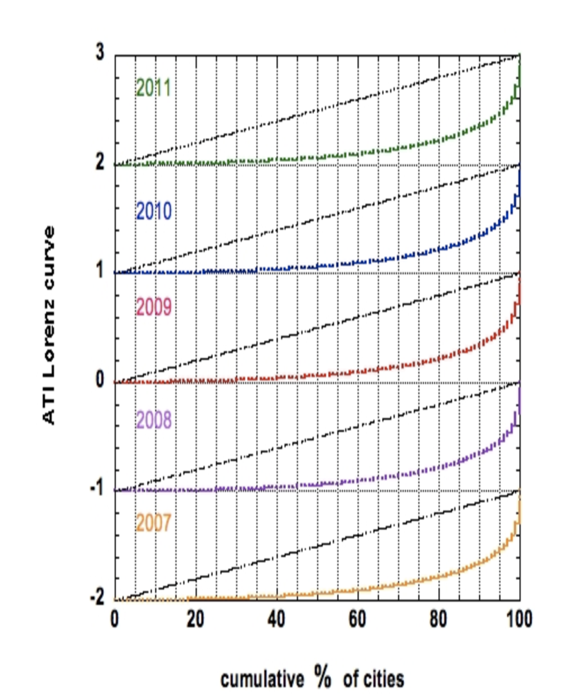
Figure 1: ATI Lorenz curve (color) and (straight) line of ATI equality (black dots) for various years of the whole set of $N$=8092 cities, i.e. all in Italy in 2011. The Gini coefficient (the values given in Table 3) is the area between those two lines. The Lorenz curves have been displaced along the $y$-axis by an obvious amount for better readability.

3 Statistical dissimilarity and competition among municipalities

This section discusses whether cities exhibit on average similar ATI values, and whenever their level of competition is high or low. For this purpose, the Theil, Gini and Herfindahl indices for each IT region are computed. All the results (necessarily numbers) are going to be presented in Tables 4-23. Nevertheless, to exemplify what a relevant corresponding figure, for these indices would be, see Fig. 1 showing the Gini case for the whole Italy. Any reader should agree that it seems unnecessary to present 20 similar figures. Further discussion is postponed to Section 4.
First, let us enter the various measure details, with defining formulae for completeness.

3.1 Theil index

The Theil index (Theil 1967) is adapted here as being defined by

$$Th=\frac{1}{N}\sum_{i=1}^{N}\frac{y_{i}}{\sum_{j}y_{j}}\cdot\ln\left(\frac{y_{i}}{\sum_{j}y_{j}}\right)$$ (3.1)

where $y_{i}$ is the ATI of the $i$-th city, and the sum $\sum_{j}y_{j}$ is the aggregation of ATI in the entire Italy, while $N$ is the number of cities ($N=8092$).
It can be easily shown, from Eq. (3.1), that the Theil index ($Th$) is given by the difference between the maximum possible entropy of the data and the observed entropy. It is a special case of the generalized entropy index. The value of the Theil index is then expressed in terms of negative entropy. Therefore, a high Theil number indicates more order that is further away from the ”ideal” maximum disorder, $ln(N)$. More specifically, a high level of Theil index is associated to a high distance from the uniform distribution of the reference variable to the elements of the sample set, which implies closeness to a polarized distribution and a high level of dispersion.
Formally, introducing the entropy:

$$H=-\sum_{i}^{N}\frac{y_{i}}{\sum_{j}y_{j}}\cdot\ln\left(\frac{y_{i}}{\sum_{j}y_{j}}\right)$$ (3.2)

where $\frac{y_{i}}{\sum_{j}y_{j}}$ is the ”market share” of the $i$-th city, it results that

$$H\;=\;ln(N)-Th\;\;or\;\;Th=ln(N)-H.$$ (3.3)

The order of magnitude of the Theil index is $Th\sim 1.73$ for the whole country; see Table 3.

3.2 Herfindahl index

The adapted Herfindahl-Hirschman index (Hirschman 1964) is formally defined as follows:

$$HHI=\sum_{i\in L_{50}}\left(\frac{y_{i}}{\sum_{j}y_{j}}\right)^{2},$$ (3.4)

where $L_{50}$ is the set of the 50 largest cities in terms of ATI, and $y_{i}$ is the ATI of the $i$-th city. The value 50 is conventional, and $HHI$ in Eq. (3.4) is the sum of the squares of the market shares of the 50 largest cities, where the market shares are expressed as fractions. The index emphasizes the weight of the largest cities. In our specific case, its value is approximately given by $7\cdot 10^{-3}$; see Table 3.
A normalized Herfindahl index is sometimes used and defined as:

$$H^{*}=\frac{\left(HHI-1/N\right)}{1-1/N}.$$ (3.5)

with the appropriate $N$. For $N$ large, $HHI\simeq H^{*}$, as it is of course for the whole country. However, except for Lombardia and Piemonte, $N$ is usually less than 600. Thus, the ”normalized” $H^{*}$ is also given in the economic index tables, for each region.

whole IT	2007	2008	2009	2010	2011	$<5yav>$
Entropy ($H$)	7.2476	7.2603	7.2659	7.2669	7.2826	7.2650
Max. Entropy	8.9986	8.9986	8.9986	8.9986	8.9986	8.9986
Theil index	$\sim 1.751$	1.7383	1.7327	1.7317	1.7160	1.7336
103 $HHI$	7.332	7.236	7.205	7.230	7.115	7.222
103 $H^{*}$	7.209	7.113	7.083	7.107	6.992	7.099
Gini Coeff.	0.7591	0.7576	0.7566	0.7565	0.7547	0.75685

Table 3: Statistical characteristics of the whole IT ATI data distribution as a function of time; $N$= 8092. Entropy is $H$ (see Eq. (3.3)); Max. Entropy $\equiv ln(8092)$; the Herfindahl index is $HHI$ (see Eq. (3.4)); the normalized Herfindahl index is $H^{*}$ (see Eq. (3.5)). Theil index is taken from Eq. (3.1).

3.3 Gini coefficient

Referring to the specific case treated here, the Gini index (Gini 1909) can be defined through the so called Lorenz curve, which (in the present case) gives the proportion $f$ of the total Italian ATI that is cumulatively provided by the bottom $x$% of the cities. If the Lorenz curve is a line at 45 degrees in an $f(x)$ plot, then there is perfect equality of ATI. The Gini index (also called coefficient ($Gi$)) is the ratio of the area that lies between the line of equality and the Lorenz curve over the total area under the line of equality.
A Gini coefficient of zero, of course, expresses perfect equality, i.e. all ATI values are the same, while a Gini coefficient equal to one (or 100%) expresses maximal inequality among values, e.g. only one city contributes to the the total Italian ATI.
For example, the IT Gini coefficient can be deduced from Fig. 1 for the whole Italy. Its yearly value, given in Table 3, is $\simeq 0.75$. It is seen that the IT $Gi$ does not much vary with time for the considered years.

3.4 Local level coefficients

Each Theil, Gini and Herfindahl index can be calculated at the country level, as presented in Table 3 and also for each IT region (or IT province). All formulae are easily transcribed. Nevertheless, for example, see how the Gini coefficient for a region reads:

$$Gi_{r}=\frac{2\sum_{i=1}^{N_{c,r}}i\;y_{i,r}}{N_{c,r}\;\sum_{i=1}^{N_{c,r}}y_{i,r}}-\frac{N_{c,r}+1}{N_{c,r}}$$ (3.6)

where $N_{c,r}$ is the number of cities in region $r$ and $y_{i,r}$ is the ATI of the $i$-th city in region $r$. Each $Gi_{r}$ is given in the corresponding 20 Tables here below for each year.
The Gini coefficient for a province would be

$$Gi_{p}=\frac{2\sum_{i=1}^{N_{c,p}}i\;y_{i,p}}{N_{c,p}\;\sum_{i=1}^{N_{c,p}}y_{i,p}}-\frac{N_{c,p}+1}{N_{c,p}}$$ (3.7)

where $N_{c,p}$ is the number of cities in province $p$ and $y_{i,p}$ is the ATI of the $i$-th city in province $p$.
Similar writings hold for the Theil and Herfindahl indices.

4 Results and discussion

This section fixes and discusses the results of the investigation. The 20 regional cases are reported in Tables 4-23. In exploring these regional cases, several facts emerge. First, it is important to note a substantial time-invariance of the values of the Theil, Herfindahl and Gini indices, which is rather expected due to not excessive length of the examined time interval.

The ranking of the Italian regions along the Theil, Gini and Herfindahl indicator values leads to the identification of several remarkable clusters. We discuss three of them.

4.1 Region clustering through index values

• Low Theil and Gini indices: Basilicata, Valle d’Aosta, Puglia and Veneto are making the bottom four.

The low levels of the Gini and Theil indicators point to regions with ”fairly distributed” ATIs. Substantially, the member cities contribute rather equally to their regional ATI. Nevertheless, within this cluster, regional cases can be quite diversified. In particular, Veneto is a region with a relevant economic core, the so called Nord-Est, with a great number of rich mid-sized cities, -in terms of population, which equally share the regional economic market. In contrast, Valle d’Aosta is the smallest (in terms of $N_{c,r}$) region of Italy: it contains only 74 municipalities (with a small number of inhabitants). A wide number of such cities are rich and comparable in terms of ATI, and this explains the fairness of the distribution of the ATI at a city level. However, Aosta -the main city- is much larger than the other municipalities, and thereby plays a predominant role (look also at the high value of the HHI index for Valle d’Aosta). Conversely, Puglia belongs to the South of Italy, and its economic structure is still in development. For the considered years, such a region appears to be made of small- and mid-sized cities, - in terms of ATI. Hence, the fair distribution of the ATIs among these municipalities describes here a generally low level of individual city ATI values.

Therefore, there can be several ”practical reasons” why an index is small, and why a cluster can be somewhat of heterogeneous nature.

• Low Herfindahl index: Emilia Romagna, Marche, Puglia and Toscana exhibit the lowest values.

This cluster mirrors different regional realities, which are however comparable in terms of the economic competition among the cities. Toscana has a large number of cultural and historical cities, attracting an enormous flow of tourism. The industrial structure of Toscana is also developed, and not polarized in a specific area. For example, Prato (a small city close to Florence) is the headquarter of a textile industrial district. Hence, the regional ATI is shared among several not much populated cities. On the other hand, Emilia Romagna has a peculiar economic characterization. The main part of the business of this region is grounded on the food industry, which is very delocalized in the entire territory. Amadori, one of the largest companies in the sector of food in Italy, has its headquarter in San Vittore di Cesena, a very small municipality close to Rimini. Yet, Bologna -the main city in Emilia Romagna- has not enough economic power to polarize the regional ATI of Emilia Romagna. Third, Puglia is a region whose economic structure is not highly developed. In this case, the lack of competition is due to an overall depressed situation. Finally, Marche has plenty of small-medium sized cities collecting extensive industrial districts. The main economic activities of this region are also in this case not concentrated in a small territory. They are principally based on clothing and shoe factories. Several brands are worldwide famous, like Diego Della Valle Tod’s (the headquarter is located at Casette d’Ete, a minuscule village close to Macerata) and Poltrona Frau (headquarter in Tolentino, a little town in the center of Marche). Ancona, the administrative center, is undoubtedly an important harbor, but with more passengers than commercial activities. Hence, Ancona is not economically powerful enough to polarize the regional ATI of Marche.
Therefore, the HHI index low value ”cluster” also implies heterogeneity, but in a different manner than the Gini and Theil index. Note that the only overlap between the two above clusters is Puglia.

• High Theil, Gini and Herfindahl indices: Lazio and Liguria assume the first two values of the rank, always, with very high values of the indices. Piemonte belongs to this cluster for what concerns Theil and Gini, but has a HHI index rather small.

In this case, statistical indicators are coherent with the Italian economical-geographical reality ”common expectation”. Lazio and Liguria are polarized regions, where the main part of the ATI is provided by a small number of cities. Specifically, there are two municipalities (Rome for Lazio and Genova for Liguria), which are remarkably predominant with respect to the other municipalities in such regions. Is it worth recalling that Rome is the capital city of Italy and encloses also Vatican City (an independent State, but with a huge percentage of Italians over the total labor force)? On the other hand, Genova holds the main commercial harbor of Italy and is the headquarter of very important companies and industrial units (one for all: Finmeccanica SPA).
The case of Piemonte is of great interest for discussing indices through this cluster . Piemonte exhibits high levels of Theil and Gini indicators, but HHI is rather small. This fact meets the evidence that Turin, with the FIAT company, provides the main part of the regional GDP. The low Herfindahl index is due to the presence -among the high-rank fifty municipalities- of a number of rich large-sized cities, but with rather few inhabitants. Indeed, Piemonte has an important industrial structure, and its economic market -in terms of ATI- is fairly shared among several competitors.
Therefore, it is shown that there is some ”practical value” in discussing the three indices in parallel for a given region.

In concluding this subsection, note that the only overlap between the two ”low index” clusters is Puglia. In some sense, it could be considered in itself as the extreme of the third cluster which have values of the indices.

4.2 Evolutions

The disorder in the yearly rankings of Italian regions for the considered indicators is due to the oscillations of the contributions that regions provide to the Italian GDP. However, the rank changes are worth to be described.

• For what concerns the Theil index, the last two in 2007 (Puglia and Veneto) interchanged their position in 2011 ($r=19\rightarrow 20$, and conversely). In so doing, Veneto lost its ever last place in the Theil index only, in 2011, but only due to the 5th decimal;

• in Theil index: Trentino Alto Adige ($r=10\rightarrow 11$) and Calabria ($r=11\rightarrow 10$);

• in Gini index: Sardegna ($r=4\rightarrow 5$) and Abruzzo ($r=5\rightarrow 4$);

• in Gini index: Sicilia ($r=7\rightarrow 8$) and Umbria ($r=8\rightarrow 7$);

• in Gini index, there is much reshuffling in row 13 to 16 between Calabria, Trentino Alto Adige, Friuli Venezia Giulia and Emilia Romagna;

• in HHI index: Campania ($r=8\rightarrow 9$) and Friuli Venezia Giulia ($r=9\rightarrow 8$);

• in HHI index: Trentino Alto Adige ($r=12\rightarrow 13$) and Lombardia ($r=13\rightarrow 12$).

The changes in the rank listed above suggest to consider the economic history of the considered regions, to grasp the reasons for such modifications. Two examples can illustrate the points:

• The case $(ii)$ can be explained by looking at the values of the Theil indices in the corresponding Tables. Trentino Alto Adige moved from 1.2823 (2007) to 1.2329 (2011), while Calabria from 1.2712 (2007) to 1.2344 (2011). The reduction of the Theil index means that in both regions a more fair income distribution has been reached, but Trentino Alto Adige was more unfair than Calabria in 2007. This result can be interpreted as follows: the current financial crisis has the merit of reducing the inequalities among the individuals, even if such fairness is attained through an overall worsening of the economic situation of Italy. The high economic level of Trentino Alto Adige, which is richer than Calabria in terms of GDP pro capite, is responsible of a more evident deterioration of the economic situation at a regional level.

• The change of position in $(vi)$ is due to a substantial invariance of the Friuli Venezia Giulia’s HHI (0.51994 in 2007, 0.51841 in 2011) and a remarkable decreasing in that of Campania (0.052596 in 2007 and 0.047086 in 2011). Campania is then over the quinquennium increasingly less polarized, which suggests the tendency of the cities to equally contribute to the regional ATI. This outcome is due to the deterioration of the regional overall economic situation, leading to the removal of the differences between the economic power of the municipalities. In this respect, we recommend the reading of the detailed report of the Bank of Italy regarding the economic situation of Campania in 2011 (Bank of Italy 2011).

4.3 Relative national impact

Finally, it is interesting to point out how the indices values fare with respect to the whole IT values. Note that

• for the Theil and Gini indices: Lazio, Liguria and Piemonte are above the Italian values of this indices, respectively;

• for the HHI index: Lazio, Liguria, but also Valle d’Aosta, Umbria and Molise are above the Italian index value, but not Piemonte.

This result is expected for Lazio, Liguria and Piemonte (see the discussion above). For what concerns Valle d’Aosta, Umbria and Molise, the datum says that a few cities highly polarize the regional index (Aosta for Valle d’Aosta, Perugia and Terni for Umbria and Campobasso and Isernia for Molise). The polarization is due to different reasons: while Valle d’Aosta -a rich region- collects a number of very small cities, leading to the predominance of Aosta (which is by itself a rather small city, but much greater than its competitors), Molise is a rather poor region where the polarization is due to concentration of all the main institutions (universities, companies’ headquarters, political institutions) in the most populated municipalities. Umbria is a particular case, because polarization is due to the contribution of Perugia -the capital of the region- but also to the presence of a very developed industrial area -including also an important plant of the Thyssenkrupp- close to Terni.

5 Conclusions

In this paper different classical economic indices have been adapted and compared in order to emphasize their relative interest in discussing city wealth contribution to a region wealth, - somewhat as a function of (recent) time. The analysis is supported through numerical application as a statistical analysis of the Italian regions for the period 2007-2011, measured by their municipalities aggregated tax income values.

Thus, it has been shown, on the IT case, that it is of interest in one hand to consider the (three) indices for a given region, and on the other hand, to consider one index for a set of regions, and compare the respective values. Moreover, it is of interest to consider the relative values with respect to the global set.

The data analysis confirms that IT is a unique entity, but with different regional realities. In particular, a detailed description of the 20 Italian regions through the Gini, Theil and Herfindahl-Hirschmann indices contribute to explain the main characteristics of the Northern and Southern regions. In particular, we concur with Mussard et al. (2003) that the Gini index attributes as much importance to the contribution between regions as to the within-regions component, whereas the Theil and Herfindahl-Hirshmann indices only consider that the inequalities are generated within the regions.

Acknowledgements

This paper is part of scientific activities in COST Action IS1104, ”The EU in the new complex geography of economic systems: models, tools and policy evaluation”.

Appendix

This Appendix contains the discussed economic indices of the 20 regional cases, in Tables 4-23.

Abruzzo	2007	2008	2009	2010	2011
Entropy	4.3501	4.3722	4.3586	4.3570	4.3634
Max. Entropy	5.7203	5.7203	5.7203	5.7203	5.7203
Theil index	1.3702	1.3481	1.3617	1.3633	1.3569
Herfindahl	0.033622	0.032324	0.032865	0.032937	0.032697
Norm. Herfindahl	0.030444	0.029141	0.029683	0.029756	0.029515
Gini Coeff.	0.750812	0.74967	0.75173	0.75212	0.75054

Table 4: Various characteristics of the ATI data for Abruzzo as a function of time; $N$= 305.

Aosta Valley	2007	2008	2009	2010	2011
Entropy	3.3003	3.3053	3.3129	3.3132	3.3204
Max. Entropy	4.3041	4.3041	4.3041	4.3041	4.3041
Theil index	1.0037	0.99880	0.99114	0.99089	0.98369
Herfindahl	0.10416	0.10330	0.10267	0.10244	0.10132
Norm. Herfindahl	0.091887	0.091017	0.090380	0.090150	0.089007
Gini Coeff.	0.64394	0.64290	0.63988	0.64020	0.63868

Table 5: Various characteristics of the ATI data for Aosta Valley as a function of time; $N$=74.

Basilicata	2007	2008	2009	2010	2011
Entropy	3.8392	3.8544	3.8569	3.8493	3.8589
Max. Entropy	4.8752	4.8752	4.8752	4.8752	4.8752
Theil index	1.0360	1.0208	1.0183	1.0259	1.0163
Herfindahl	0.060062	0.058582	0.058448	0.059088	0.058246
Norm. Herfindahl	0.052831	0.051341	0.051205	0.051850	0.051002
Gini Coeff.	0.64826	0.64559	0.64498	0.64674	0.64461

Table 6: Various characteristics of the ATI data for Basilicata as a function of time; $N$= 131.

Calabria	2007	2008	2009	2010	2011
Entropy	4.7425	4.7614	4.7704	4.7729	4.7793
Max. Entropy	6.0137	6.0137	6.0137	6.0137	6.0137
Theil index	1.2712	1.2523	1.2434	1.2408	1.2344
Herfindahl	0.031257	0.030534	0.030101	0.029947	0.029500
Norm. Herfindahl	0.028882	0.028158	0.027723	0.027569	0.027121
Gini Coeff.	0.68512	0.68231	0.68072	0.68040	0.68055

Table 7: Various characteristics of the ATI data for Calabria as a function of time; $N$= 409.

Campania	2007	2008	2009	2010	2011
Entropy	4.7335	4.7655	4.7739	4.7765	4.8062
Max. Entropy	6.3117	6.3117	6.3117	6.3117	6.3117
Theil Index	1.5783	1.5463	1.5378	1.5352	1.5056
Herfindahl	0.052596	0.049981	0.049289	0.049167	0.047086
Norm. Herfindahl	0.050873	0.048253	0.047561	0.047438	0.045354
Gini Coeff.	0.74246	0.73900	0.73812	0.73765	0.73390

Table 8: Various characteristics of the ATI data for Campania as a function of time; $N$= 551.

Emilia Romagna	2007	2008	2009	2010	2011
Entropy	4.6856	4.7011	4.7002	4.7032	4.7090
Max. Entropy	5.8319	5.8522	5.8522	5.8522	5.8522
Theil index	1.1463	1.1511	1.1520	1.1490	1.1432
Herfindahl	0.026274	0.025869	0.025875	0.025711	0.025425
Norm. Herfindahl	0.02341	0.023061	0.023068	0.022904	0.022617
Gini Coeff.	0.68118	0.68272	0.68254	0.68209	0.68066

Table 9: Various characteristics of the ATI data for Emilia Romagna as a function of time; $N$= 341 in 2007, and 348 next.

Friuli Venetia Giulia	2007	2008	2009	2010	2011
Entropy	4.1877	4.1849	4.179864	4.1799	4.1935
Max. Entropy	5.3891	5.3845	5.384495	5.3845	5.3845
Theil index	1.2014	1.1996	1.2046	1.2046	1.1910
Herfindahl	0.051994	0.052270	0.052972	0.052852	0.051841
Norm. Herfindahl	0.047646	0.047902	0.048607	0.048487	0.047471
Gini Coeff.	0.68181	0.68135	0.681851	0.68228	0.67983

Table 10: Various characteristics of the ATI data for Friuli Venetia Giulia a function of time; $N$ depends on year. It is 219 in 2007, and 218 next.

Lazio	2007	2008	2009	2010	2011
Entropy	2.6121	2.6297	2.6458	2.6442	2.6664
Max. Entropy	5.9349	5.9349	5.9349	5.9349	5.9349
Theil index	3.3228	3.3052	3.2891	3.2906	3.2685
Herfindahl	0.37093	0.36688	0.36337	0.36350	0.35877
Norm. Herfindahl	0.36926	0.36520	0.36168	0.36181	0.35707
Gini Coeff.	0.88065	0.87985	0.87891	0.87927	0.87790

Table 11: Various characteristics of the ATI data for Lazio as a function of time; $N$= 378.

Liguria	2007	2008	2009	2010	2011
Entropy	3.1712	3.1775	3.1859	3.1875	3.2039
Max. Entropy	5.4596	5.4596	5.4596	5.4596	5.4596
Theil index	2.2884	2.2821	2.2737	2.2721	2.2557
Herfindahl	0.19257	0.19169	0.19060	0.19010	0.18758
Norm. Herfindahl	0.18912	0.18824	0.18714	0.18664	0.18411
Gini Coeff.	0.83346	0.83257	0.83133	0.83143	0.82956

Table 12: Various characteristics of the ATI data for Liguria as a function of time; $N$= 235.

Lombardia	2007	2008	2009	2010	2011
Entropy	5.6933	5.7056	5.7140	5.7135	5.7239
Max. Entropy	7.3434	7.3434	7.3434	7.3421	7.3421
Theil index	1.6501	1.6379	1.6294	1.6287	1.6182
Herfindahl	0.038857	0.038179	0.037639	0.037805	0.037402
Norm. Herfindahl	0.038235	0.037556	0.037016	0.037181	0.036779
Gini Coeff.	0.71799	0.71688	0.71592	0.71544	0.71405

Table 13: Various characteristics of the ATI data for Lombardia as a function of time; $N$= 1546 in 2007-09, and becomes 1544 next.

Marche	2007	2008	2009	2010	2011
Entropy	4.4416	4.4179	4.4165	4.4212	4.4328
Max. Entropy	5.5053	5.4765	5.4765	5.4765	5.4765
Theil index	1.0638	1.0586	1.0600	1.0552	1.0436
Herfindahl	0.024916	0.025284	0.025419	0.025215	0.024742
Norm. Herfindahl	0.020936	0.021189	0.021324	0.021119	0.020644
Gini Coeff.	0.70161	0.70162	0.70152	0.70082	0.69835

Table 14: Various characteristics of the ATI data for Marche as a function of time; $N$= 239.

Molise	2007	2008	2009	2010	2011
Entropy	3.6245	3.6314	3.6371	3.6407	3.6396
Max. Entropy	4.9127	4.9127	4.9127	4.9127	4.9127
Theil index	1.2882	1.2813	1.2756	1.2719	1.2730
Herfindahl	0.076722	0.076097	0.076336	0.076014	0.075998
Norm. Herfindahl	0.069883	0.069253	0.069494	0.069170	0.069153
Gini Coeff.	0.70074	0.69894	0.69593	0.69571	0.69669

Table 15: Various characteristics of the ATI data for Molise as a function of time; $N$= 136.

Piemonte	2007	2008	2009	2010	2011
Entropy	5.0806	5.0873	5.0974	5.1005	5.1240
Max. Entropy	7.0951	7.0951	7.0951	7.0951	7.0951
Theil index	2.0145	2.0077	1.9977	1.9946	1.9711
Herfindahl	0.056106	0.055743	0.054883	0.054699	0.053053
Norm. Herfindahl	0.055323	0.054959	0.054099	0.053914	0.052267
Gini Coeff.	0.78607	0.78524	0.78395	0.78380	0.78179

Table 16: Various characteristics of the ATI data for Piemonte as a function of time; $N$= 1206.

Puglia	2007	2008	2009	2010	2011
Entropy	4.5759	4.5907	4.5987	4.6018	4.6148
Max. Entropy	5.5530	5.5530	5.5530	5.5530	5.5530
Theil index	0.9770	0.9622	0.9542	0.9512	0.9381
Herfindahl	0.027864	0.027173	0.026807	0.026671	0.026025
Norm. Herfindahl	0.024082	0.023388	0.023020	0.022884	0.022235
Gini Coeff.	0.65401	0.65077	0.64895	0.64841	0.64556

Table 17: Various characteristics of the ATI data for Puglia as a function of time; $N$= 258.

Sardegna	2007	2008	2009	2010	2011
Entropy	4.4108	4.4302	4.4407	4.4405	4.4486
Max. Entropy	5.9322	5.9322	5.9322	5.9322	5.9322
Theil index	1.5215	1.5020	1.4915	1.4918	1.4836
Herfindahl	0.042023	0.040887	0.040300	0.040363	0.039878
Norm. Herfindahl	0.039475	0.038336	0.037747	0.037810	0.037325
Gini Coeff.	0.75202	0.74918	0.74738	0.74760	0.74684

Table 18: Various characteristics of the ATI data for Sardegna as a function of time; $N$= 377.

Sicilia	2007	2008	2009	2010	2011
Entropy	4.4933	4.5243	4.5327	4.5351	4.5584
Max. Entropy	5.9661	5.9661	5.9661	5.9661	5.9661
Theil index	1.4729	1.4418	1.4335	1.4310	1.4077
Herfindahl	0.045118	0.043540	0.043014	0.042918	0.041555
Norm. Herfindahl	0.042664	0.041081	0.040554	0.040457	0.039091
Gini Coeff.	0.73536	0.73044	0.72899	0.72878	0.72502

Table 19: Various characteristics of the ATI data for Sicilia as a function of time; $N$= 390.

Toscana	2007	2008	2009	2010	2011
Entropy	4.5757	4.5809	4.5860	4.5875	4.5959
Max. Entropy	5.6595	5.6595	5.6595	5.6595	5.6595
Theil index	1.0838	1.0786	1.0735	1.0719	1.0636
Herfindahl	0.028356	0.028135	0.027904	0.027858	0.027605
Norm. Herfindahl	0.024959	0.024737	0.024505	0.024459	0.024205
Gini Coeff.	0.68612	0.68493	0.68342	0.68303	0.68126

Table 20: Various characteristics of the ATI data for Toscana as a function of time; $N$= 287.

Trentino Alto Adige	2007	2008	2009	2010	2011
Entropy	4.5437	4.5386	4.5527	4.5619	4.5753
Max. Entropy	5.8260	5.8081	5.8081	5.8081	5.8081
Theil Index	1.2823	1.2695	1.2555	1.2462	1.2329
Herfindahl	0.039446	0.039042	0.038398	0.037800	0.036930
Norm. Herfindahl	0.036605	0.036147	0.035502	0.034902	0.034029
Gini Coeff.	0.68340	0.68286	0.68017	0.67910	0.67741

Table 21: Various characteristics of the ATI data for Trentino Alto Adige as a function of time; $N$=333.

Umbria	2007	2008	2009	2010	2011
Entropy	3.3039	3.3074	3.3119	3.3117	3.3236
Max. Entropy	4.5218	4.5218	4.5218	4.5218	4.5218
Theil index	1.2179	1.2144	1.2099	1.2101	1.1982
Herfindahl	0.083292	0.082894	0.082372	0.082275	0.080978
Norm. Herfindahl	0.073219	0.072816	0.072288	0.072190	0.070879
Gini Coeff.	0.73213	0.73151	0.73072	0.73131	0.72907

Table 22: Various characteristics of the ATI data for Umbria as a function of time; $N$= 92.

Veneto	2007	2008	2009	2010	2011
Entropy	5.4028	5.4088	5.4073	5.4124	5.4266
Max. Entropy	6.3648	6.3648	6.3648	6.3648	6.3648
Theil index	0.9619	0.9559	0.9574	0.9524	0.9381
Herfindahl	0.015352	0.015143	0.015164	0.015013	0.014591
Norm. Herfindahl	0.013654	0.013445	0.013466	0.013314	0.012892
Gini Coefficient	0.61816	0.61755	0.61821	0.61733	0.61476

Table 23: Various characteristics of the ATI data for Veneto as a function of time; $N$= 581.

References

- [1] Alvarado, F.L., 1999, Market Power: a dynamical definition, Strategic Management Journal 20, 969-975
- [2] Aristondo, O., Garc a-Lapresta, J.L., Lasso de la Vega, C., Marques Pereira, R.A., 2012. The Gini index, the dual decomposition of aggregation functions, and the consistent measurement of inequality. International Journal of Intelligent Systems 27(2), 132-152.
- [3] Bagatella-Flores, N., Rodríguez-Achach, M., Coronel-Brizio,H.F. , Hernández-Montoya, A.R. 2014, Wealth distribution of simple exchange models coupled with extremal dynamics. (Unpublished manuscript available at) .
- [4] Bank of Italy, 2011, Economie regionali - L’economia della Campania. Centro Stampa della Banca d’ IItalia.
- [5] Bartels, L., Unequal Democracy: The Political Economy of the New Gilded Age. Princeton University Press: Princeton, 2008.
- [6] Clippe, P., Ausloos, M., 2012. Benford’s law and Theil transform of financial data, Physica A 391(24), 6556-6567.
- [7] Fan, C.C., Sun, M., 2008. Regional Inequality in China, 1978-2006, Eurasian Geography and Economics 49(1), 1-20.
- [8] Gini, C., 1909. Concentration and dependency ratios (in Italian). English translation in Rivista di Politica Economica 87 (1997), 769-789.
- [9] Hirschman, A.O., 1964. The paternity of an index, The American Economic Review 54(5), 761-762.
- [10] Iglesias, J. R., de Almeida, R.M. C. 2012, Entropy and equilibrium state of free market models, European Journal of Physics B 85, 1-10.
- [11] Miskiewicz, J., 2008. Globalization Entropy unification through the Theil index, Physica A 387(26), 6595-6604.
- [12] Mussard, S., Seyte, Fr., Terraza, M. 2003. Decomposition of Gini and the generalized entropy inequality measures. Economics Bulletin, 4 (7) 1-6.
- [13] Essama-Nssah, B., 1997. Impact of growth and distribution on poverty in madagascar, Review of Income and Wealth 43(2), 239 252.
- [14] Psacharopoulos, G., Morley, S., Fiszbein, A., Lee, H., Wood, W.C., 1995. Poverty and income inequality in latin america during the 1980s, Review of Income and Wealth 41(3), 245 264.
- [15] Rotundo, G., D’Arcangelis, A.M., 2014. Network of companies: an analysis of market concentration in the Italian stock market, Quality and Quantity 48 (4), 1893-1910.
- [16] Souma, R., 2002. Physics of Personal Income, in Empirical Science of Financial Fluctuations, H. Takayasu ed, (Springer) pp. 343–352
- [17] Theil, H., 1967. Economics and Information Theory, Chicago: Rand McNally and Company.
- [18] Walks, A., 2013. Income Inequality and Polarization in Canada’s Cities: An Examination and New Form of Measurement, Research Paper 227, Neighbourhood Change Research Partnership, University of Toronto, August 2013.
- [19] Wan, G., Lu, M., Chen, Z., 2007. Globalization and regional income inequality: empirical evidence from within china, Review of Income and Wealth 53(1), 35 59.