Non-Gaussian features from Excited Squeezed Vacuum State

Abstract

In this work, we introduce a non-Gaussian quantum state named excited squeezed vacuum state (ESVS), which can be ustilized to describe quantum light field emitted from the multiphoton quantum process occurred in some restricted quantum systems. We investigate its nonclassical properties such as Wigner distribution in phase space, photon number distribution, the second-order autocorrelation and the quadrature fluctuations. By virtue of the Hilbert-Schmidt distance method, we quantify the non-Gaussianity of the ESVS. Due to the similar photon statistics, we examine the fidelity between the ESVS and the photon-subtraction squeezed vacuum state (PSSVS), and then find the optimal fidelity by monitoring the relevant parameters.

PACS numbers: 42.50.Dv, 03.67. a, 42.50.Ex

1 Introduction

Current research suggests that non-Gaussian states, endowed with the qualitative role of quantum coherence or entanglement for revealling the fascinating quantum phenomena, can preserve their nonclassicality much better than Gaussian ones in quantum information process (QIP). Also non-Gaussian operations become an essential ingredient for some quantum tasks such as entanglement distillation [1, 2] and noiseless amplication [3]. To say the least, non-Gaussian regime has powerfully extended to quantum information tasks, e.g. metrology [4], cloning [5], communication [6], computation [7, 8] and testing of quantum theory [9].

In the frame of non-Gaussian mechanism, much attention has been foused on generation schemes [10, 11, 12, 13, 14], nonclassicality investigation [15, 16, 17], quantum protocols [18, 19, 20]. In general, due to the lack of high order nonlinearity, it is very difficult to deterministically generate non-Gaussian states of light via optical material media. Quantum systems with restricted dimensions have proved to be fertile ground for discovering non-Gaussian light. For instance, in a coupled cavity-atom system an extra resonance has been observed as well as vacuum Rabi resonance [21]. In a photonic crystal cavity containing a strongly coupled quantum dot, authors have discovered the photon-induced tunneling phenomena, which is a nonclassical transmitted light [22]. In circuit quantum electrodynamics (QED), the giant self-Kerr effect can be detected by measuring the second-order correlation function and quadrature squeezing spectrum [23]. In those coupled microscopic quantum systems, strong interactions can generate highly nonclassical light, which has possible uses in quantum communication [24] and metrology [25].

One important question that arises is how to describe quantum states of nonclassical light emitted from the restricted quantum system. Due to strong coupling, the composite system consisting of a multi-level atom (or quantum dot) coupled to a cavity and driven by a weak coherent field, can be described as Jaynes-Cummings (JC) model. Quantum-optical effects can be demonstrated in the interaction processes of photon emission and absorbtion with atom between ground and excited states. Its energy-level structure is discrete, so-called the dressed states [26, 27], which is an overall description of evalution. Multi-photon processes originated from quantum nonlinearity can be monitored via the fluorescent resonance [28, 29, 30] and the other extra resonance [31]. Only considering an effective measurement to optical field, photon-statistics methods [22], such as the second-order coherence function at time delay zero $g^{\left(2\right)}\left(0\right)=\frac{\left\langle a^{{\dagger}}a^{{\dagger}}aa\right\rangle}{\left\langle a^{{\dagger}}a\right\rangle^{2}}$ or high order differential correlation function $C^{\left(n\right)}\left(0\right)=\left\langle a^{{\dagger}n}a^{n}\right\rangle-\left\langle a^{{\dagger}}a\right\rangle^{n},$ are often utilized to study nonclassical characteristics of emitting light. For the case of weak coherent incident field, the quantum state of emitted light can be expressed as a series of excited coherent states $\sum_{m}C_{m}a^{{\dagger}m}\left|\alpha\right\rangle$ or a superposition of the different Fock states $\left|\psi\right\rangle=\sum_{n}C_{n}\left|n\right\rangle$ (due to $\left|\alpha\right\rangle=\sum_{n}\frac{\alpha^{n}}{\sqrt{n!}}\left|n\right\rangle$) [22]. Its photon-statistics can exhibit similar behavior to that of an excited quantum state (e.g. $a^{{\dagger}m}\left|\varphi\right\rangle$).

It is interesting to consider a single-mode squeezed vacuum field to be an initial state of the incident source. Therefore, abundant nonclassicality of emitting field can be demonstrated by studying excited squeezed vacuum state (ESVS). In Ref.[32], considering the interaction of a two-level atom with a squeezed vacuum, authors have calculated the second-order intensity correlation function, the spectrum of squeezing, the coherent spectrum and discussed nonclassical behavior of light field. Similar issues have been addressed in Refs.[33, 34, 35, 36, 37, 38]. A recent experimental study found a twofold reduction of the transverse radiative decay rate of a superconducting artificial atom coupled to continuum squeezed vacuum [39]. More attention has been paid to investigate Wigner function and tomogram of ESVS in Ref. [40, 15, 16, 17]. In this work, we focus on a single-mode squeezed vacuum field with any number of photon addition, and investigate its nonclassical properties. In Sec. II, by virtue of quantum phase space technique, we derive an analytical expression of quasi-probability distribution Wigner function, negativity of which can exhibit nonclassical behavior of the ESVS. And then we investigate its photon number statistics, calculate the Mandel’s $Q$ parameter, examine the quadrature fluctuations $\left\langle\Delta X\right\rangle,$ $\left\langle\Delta Y\right\rangle$ and the correlation $\left\langle\Delta X\right\rangle\left\langle\Delta Y\right\rangle,$ which can be measured outside the cavity by using a homodyne detection with a controllable phase. In Sec. III, we evaluate its non-Gaussianity via the Hilbert-Schmidt distance method [41]. As results, we shall study how the photon number modulation affects the non-Gaussianity of the ESVS and provide a guide to enhance non-Gaussianity of a desired quantum state. It is found that photon number distribution of the ESVS is similar to that of the photon-subtraction squeezed vacuum state (PSSVS). Fidelity between the ESVE and the PSSVS is obtained and the optimal fidelity has been discussed in Sec. IV. We end with the main conclusions of our work.

2 Nonclassical Properties Investigation of the ESVS

As is well known, a single mode squeezed field is an approximation with a superposition of all even number photon states, i.e.,

$$S\left(r\right)\left|0\right\rangle=\exp\left[\frac{r}{2}\left(a^{{\dagger}2}-a^{2}\right)\right]\left|0\right\rangle=\frac{1}{\sqrt{\cosh r}}\sum_{n=0}\left(-1\right)^{n}\frac{\sqrt{\left(2n\right)!}}{2^{n}n!}\tanh^{n}r\left|2n\right\rangle,$$ (1)

in which $r$ is the squeezing parameter. Adding one single photon to a weak squeezed field can be described by

$$a^{{\dagger}}S\left(r\right)\left|0\right\rangle\rightarrow\sum_{n=0}\left(-1\right)^{n}\frac{\sqrt{\left(2n+1\right)!}}{2^{n}n!}\tanh^{n}r\left|2n+1\right\rangle,$$ (2)

which is a superposition of all odd number photon states. Theoretically, by repeating ($n$ times) application of the photon creation operator $a^{{\dagger}}$ on the squeezed vacuum field, we can obtain the excited squeezed vacuum state (ESVS) $a^{{\dagger}n}S\left(r\right)\left|0\right\rangle.$ For the case of small value of $n$, the ESVS can be generated via the spontaneous parametric down-conversion (SPDC) occured in nonlinear optical media or the multiphoton processes in above-mentioned restricted quantum systems. Thus its density operator reads

$$\rho\left(r,n\right)=C_{n}^{-1}a^{{\dagger}}{}^{n}S\left(r\right)\left|0\right\rangle\left\langle 0\right|S^{-1}\left(r\right)a^{n}\equiv C_{n}^{-1}a^{{\dagger}}{}^{n}\rho\left(r\right)a^{n},$$ (3)

in which $\rho\left(r\right)\equiv S\left(r\right)\left|0\right\rangle\left\langle 0\right|S^{-1}\left(r\right)$ denotes the squeezed vacuum field, $C_{n}=Tr\left[\rho\left(r,n\right)\right]=n!\cosh^{n}rP_{n}\left(\cosh r\right)$ is a normalized constant. $P_{n}\left(\cosh r\right)$ is the expression of the Legendre polynomials and this result has also obtained in Ref.[40].

2.1 Quasi-probability Distribution: Wigner Function

In order to interview the nonclassical properties of a quantum light fields, the Wigner function, although not positive definition in general, provides a closely parallel interpretation as a probability distribution function. Based on the Weyl’s mapping rule [42, 43], the classical correspondence of density operator $\rho$ is just the Wigner function, namely

$$\rho=\int\int_{-\infty}^{\infty}dqdp\Delta\left(q,p\right)W\left(q,p\right)$$ (4)

or

$$W\left(q,p\right)=Tr\left[\rho\Delta\left(q,p\right)\right],$$ (5)

$W\left(q,p\right)$ is the Wigner function of $\rho$ and $\Delta\left(q,p\right)$ denotes the Wigner operator, defined in the coordinate representation $\left|q\right\rangle$ as

$$\Delta\left(p,q\right)=\int_{-\infty}^{\infty}\frac{dv}{2\pi}e^{ipv}\left|q+\frac{v}{2}\right\rangle\left\langle q-\frac{v}{2}\right|.$$ (6)

Noting that $\alpha=\frac{1}{\sqrt{2}}\left(q+ip\right),$ we can see $W\left(\alpha,\alpha^{\ast}\right)=Tr\left[\rho\Delta\left(\alpha,\alpha^{\ast}\right)\right],$ where

$$\Delta\left(\alpha,\alpha^{\ast}\right) = \int\frac{d^{2}z}{\pi^{2}}\left|\alpha+z\right\rangle\left\langle\alpha-z\right|e^{\alpha z^{\ast}-\alpha^{\ast}z}=\frac{1}{\pi}\colon\exp\left[-2\left(a^{\dagger}-\alpha^{\ast}\right)\left(a-\alpha\right)\right]\colon$$ (9)

$$= \frac{1}{2}\begin{array}[]{c}\dot{\vdots}\end{array}\delta\left(\alpha-a\right)\delta\left(\alpha^{\ast}-a^{\dagger}\right)\begin{array}[]{c}\dot{\vdots}\end{array},$$

$\left\langle z\right|=\left\langle 0\right|\exp\left[-\frac{1}{2}|z|^{2}+z^{\ast}a\right]$ is the Glauber coherent state [44], the symbols ’ $\colon\colon$’ and ’$\begin{array}[]{c}\dot{\vdots}\end{array}\begin{array}[]{c}\dot{\vdots}\end{array}$’denote the normal ordering and Weyl ordering, repectively. In particular, a unitary operator (e.g. $S$ with its identities $SaS^{-1}=\mu a+\nu a^{\dagger},$ $Sa^{\dagger}S^{-1}=\sigma a+\tau a^{\dagger})$ can ’run across’ the ’border’ of ’$\begin{array}[]{c}\dot{\vdots}\end{array}\begin{array}[]{c}\dot{\vdots}\end{array}$’ and directly transforms bosonic operators, i.e.

$$SF\left(a^{\dagger},a\right)S^{-1}=F\left(\mu a+\nu a^{\dagger},\sigma a+\tau a^{\dagger}\right)=\begin{array}[]{c}\dot{\vdots}\end{array}f\left(\mu a+\nu a^{\dagger},\sigma a+\tau a^{\dagger}\right)\begin{array}[]{c}\dot{\vdots}\end{array},$$ (10)

which also named the Weyl ordering invariance under similarity transformations [45]. Substituting Eq.(3) into Eq.(5), we can derive the Wigner function of the ESVS, namely

$$W\left(\alpha,\alpha^{\ast}\right) = \frac{1}{P_{n}\left(\cosh r\right)}\left(\frac{\sinh r}{2}\right)^{n}\exp\left[-2\left|\alpha\cosh r-\alpha^{\ast}\sinh r\right|^{2}\right]$$ (11)

$$\times\sum_{m=0}^{n}\binom{n}{m}\left(-2\coth r\right)^{m}\left|H_{n-m}\left[-i\sqrt{\frac{2}{\tanh r}}\left(\alpha\cosh r-\alpha^{\ast}\sinh r\right)\right]\right|^{2},$$

where $H_{n}\left(x\right)$ is the Hermite polynomials defined as

$$H_{n}\left(x\right)=x^{n}\sum_{k=0}^{\left[n/2\right]}\frac{n!}{2^{2k}\left(k!\right)^{2}\left(n-2k\right)!}\left(1-\frac{1}{x^{2}}\right)^{k}.$$ (12)

As we can see in Eq.(11), the exponential function $\exp\left[-2\left|\alpha\cosh r-\alpha^{\ast}\sinh r\right|^{2}\right]$ is a discription of Gaussian distribution and the Wigner function $W\left(\alpha,\alpha^{\ast}\right)$ of the ESVS is a sum of products of the Hermite-Gaussian functions. Details in the derivation of Eq.(11) has been shown in Appendix A.

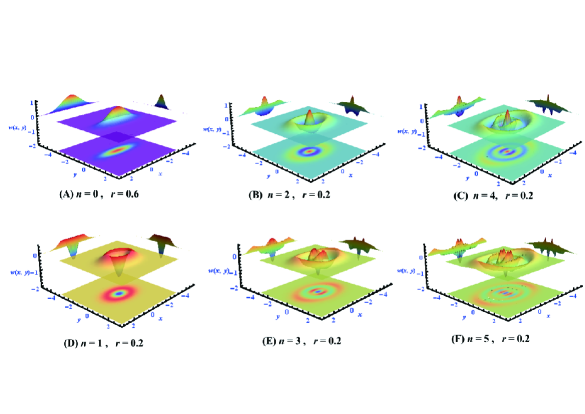
Figure 1: Wigner functions of the ESVS with fixed $n$ and $r$ : (A). $n=0,$ $r=0.6,$ (B). $n=2,$ $r=0.2,$ (C). $n=4,$ $r=0.2,$ (D). $n=1,$ $r=0.2,$ (E). $n=3,$ $r=0.2,$ (F). $n=5,$ $r=0.2.$ In the top row, Figure 1(A) exhibits a squeezed vacuum state, and in Figure 1(B)–1(C) adding even photon shows a a smaller positive value at the center. In the bottom row (Figure 1(D)–1(F)), adding odd photon leads to a negative value at the center of phase space. More added-photon means a much more complex distribution.

Figure 1 shows the quantum non-Gaussian states can be preapred by adding photon to a weak light field. At low intensities of the squeezed vacuum field (see Figure 1(A)), the variance of photon-addition can exhibit different nonclassical features (negative distribution). (B) and (C) describe the even photon-addition states, odd photon-addition states in (D), (E) and (F). Indeed, the squeezing parameter $r$ dominates the quadrature distribution in the directions of $-X$ and $-Y$. Here the values of $r$ are $0.6$ in (A) and $0.2$ in (B)-(F), respectively.

2.2 Photon Number Distribution

In Eq.(3), noting that $\left|0\right\rangle\left\langle 0\right|=\colon\exp\left(-a^{{\dagger}}a\right)\colon,$ we have

$$\rho\left(r\right)\equiv S\left(r\right)\left|0\right\rangle\left\langle 0\right|S^{-1}\left(r\right)=\frac{1}{\cosh r}\colon\exp\left[\frac{1}{2}a^{{\dagger}2}\tanh r+\frac{1}{2}a^{2}\tanh r-a^{{\dagger}}a\right]\colon$$ (13)

Photon number distribution (PND) of the ESVS can be defined via the probability of finding $m$ photons, namely

$$P_{m}\left(r,n\right) = \left\langle m\right|\rho\left(r,n\right)\left|m\right\rangle$$ (14)

$$= C_{n}^{-1}\frac{1}{\cosh r}\frac{m!}{\left(m-n\right)!}\left\langle m-n\right|\colon\exp\left[\frac{1}{2}a^{{\dagger}2}\tanh r+\frac{1}{2}a^{2}\tanh r-a^{{\dagger}}a\right]\colon\left|m-n\right\rangle.$$

And using $\left|n\right\rangle=\frac{1}{\sqrt{n!}}\left.\frac{d^{n}}{d\alpha^{n}}\left|\alpha\right\rangle\right|_{\alpha=0}$ , $\left\langle\beta\right.\left|\alpha\right\rangle=\exp\left(\alpha\beta^{\ast}\right)$ and the differential form of the Hermite polynomials

$$H_{n}\left(x\right)=\left(-1\right)^{n}e^{x^{2}}\frac{d^{n}}{dx^{n}}e^{-x^{2}},$$ (15)

we have

$$P_{m}\left(r,n\right) = C_{n}^{-1}\frac{1}{\cosh r}\frac{m!}{\left[\left(m-n\right)!\right]^{2}}\left.\frac{d^{m-n}}{d\beta^{\ast m-n}}\frac{d^{m-n}}{d\alpha^{m-n}}\exp\left[\frac{1}{2}\beta^{\ast 2}e^{-i\theta}\tanh r+\frac{1}{2}\alpha^{2}e^{i\theta}\tanh r\right]\right|_{\alpha,\beta^{\ast}=0}$$ (16)

$$= C_{n}^{-1}\frac{1}{\cosh r}\frac{m!}{\left[\left(m-n\right)!\right]^{2}}\left(-\frac{\tanh r}{2}\right)^{m-n}\left[H_{m-n}\left(0\right)\right]^{2},$$

where $C_{n}\$is given in Eq.(3). For the case of $x=0,$ we can see

$$H_{2n}\left(0\right)=\left(-1\right)^{n}\frac{\left(2n\right)!}{n!},\text{ \ \ \ }H_{2n+1}\left(0\right)=0.$$ (17)

Therefore, the results of $P_{m}\left(r,n\right)$ can be decided by the value of $m-n.$ Noting a differential identity for the Legendre polynomials, i.e.

$$\left.\frac{\partial{}^{2m}}{\partial t{}^{m}\partial\tau{}^{m}}\exp\left[-t{}^{2}-\tau{}^{2}+\frac{2xt\tau}{\sqrt{x^{2}-1}}\right]\right|_{t,\tau=0}=\frac{2^{m}m!}{\left(x^{2}-1\right)^{m/2}}P_{m}\left(x\right),$$ (18)

we can rewrite Eq.(16) as

$$P_{m}\left(r,n\right) = \frac{C_{n}^{-1}}{\cosh r}\frac{m!}{\left[\left(m-n\right)!\right]^{2}}\left(-\frac{\tanh r}{2}\right)^{m-n}\left.\frac{d^{m-n}}{d\beta^{\ast m-n}}\frac{d^{m-n}}{d\alpha^{m-n}}\exp\left[-\beta^{\ast 2}-\alpha^{2}\right]\right|_{\alpha,\beta^{\ast}=0}$$ (19)

$$= \frac{C_{n}^{-1}}{\cosh r}\left(-\frac{\tanh r}{2}\right)^{m-n}\frac{m!}{\left(m-n\right)!}\frac{2^{m-n}}{\left(-1\right)^{(m-n)/2}}P_{m-n}\left(0\right).$$

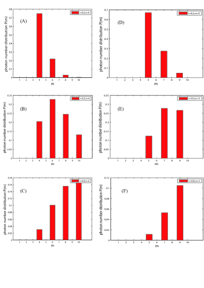
Figure 2: Photon number distributions of the ESVE with fixed added-photon number $n.$ Enhancing squeezing leads to the transition of photon number probability distribution from the left column (Figure 2(A)–2(C)) with $n=4$ and $r=0.2,$ $0.5,$ $0.8,$ to the right (Figure 2(D)–2(F)) with $n=5$ and $r=0.2,$ $0.5,$ $0.8$.

Indeed, the squeezed vacuum field is close to the even number photon superposition states. For the case of an odd photon-addition, the final state can be described by an odd photon superposition states, for details see Eq.(43) in Sec. IV. This point has also been shown on the right column of Figure 2. When rising value of the squeezing parameter $r,$ we can see that the probability distribution has gradually transited towards to the larger photon number distribution (see from figure 2(D) to figure 2(E)). If adding even photon, this distribution can be described by an even photon superposition states, as you can see on the left column of Figure 2. For the case of an odd photon-addition, the similar results can also be obtained by enhancing the squeezing $r$ (see from Figure 2(A) to 2(C)).

2.3 Mandel’s $Q$ Parameter

In order to show the occupation of photon number distribution, the above mentioned second-order coherence function at time delay zero $g^{\left(2\right)}\left(0\right)$ is often utilized to measure the nonclassicality of quantum light. Alternatively, Ref.[46] defined the Mandel’s $Q$ parameter,

$$Q=\frac{\left\langle a^{{\dagger}2}a^{2}\right\rangle}{\left\langle a^{{\dagger}}a\right\rangle}-\left\langle a^{{\dagger}}a\right\rangle=\frac{\left\langle\hat{n}^{2}\right\rangle-\left\langle\hat{n}\right\rangle^{2}}{\left\langle\hat{n}\right\rangle}-1=\left\langle\hat{n}\right\rangle\left[g^{\left(2\right)}\left(0\right)-1\right]$$ (20)

to characterize nonclassicality with negative values indicating a sub-Poissonian statistics in resonance fluorescence. The minimal value $Q=-1$ indicates the photon number states and $-1\leq Q<0$ can be interpreted as a nonclassical probability distribution. $Q=0$ means a Poissonian photon number statistics, which is mostly close to the classical probability distribution (e.g. coherent state). For the case of $Q>0,$ light field is considered to be the super-Poissonian distribution. From Eq. (3) and noting that

$$\left\langle a^{{\dagger}}a\right\rangle = \left\langle\lambda,n\right|a^{{\dagger}}a\left|\lambda,n\right\rangle=C_{n}^{-1}\left\langle 0\right|S^{-1}\left(\lambda\right)a{}^{n}a^{{\dagger}}aa^{{\dagger}}{}^{n}S\left(\lambda\right)\left|0\right\rangle=\frac{C_{n+1}-C_{n}}{C_{n}},$$

$$\left\langle a^{{\dagger}2}a^{2}\right\rangle = \left\langle\lambda,n\right|a^{{\dagger}2}a^{2}\left|\lambda,n\right\rangle=C_{n}^{-1}\left\langle 0\right|S^{-1}\left(\lambda\right)a{}^{n}a^{{\dagger}2}a^{2}a^{{\dagger}}{}^{n}S\left(\lambda\right)\left|0\right\rangle=\frac{C_{n+2}}{C_{n}}-4\frac{C_{n+1}}{C_{n}}+2,$$ (21)

the Mandel’s Q parameter is given by

$$Q=\frac{\left\langle a^{{\dagger}2}a^{2}\right\rangle}{\left\langle a^{{\dagger}}a\right\rangle}-\left\langle a^{{\dagger}}a\right\rangle=\frac{C_{n+2}-2C_{n}}{C_{n+1}-C_{n}}-\frac{C_{n+1}}{C_{n}}-3,$$ (22)

where coeffcient $C_{n+j}=\left(n+j\right)!\cosh^{n+j}rP_{n+j}\left(\cosh r\right)$ has defined in Eq.(3). As a function of parameters $n$ and $r$, the Mandel’s $Q$  has been shown in Figure 3(A). From the top to bottom, the values of $n$ are fixed with $0$, $1$ and $6$. For the case of $n=0,$ $Q\geqslant 1$ means the squeezing vacuum field has super-Poissonian photon statistics (see orange line in Figure 3(A)). Besides $n=0,$ the ESVS is sub-Poissonian, Poissonian and super-Poissonian with the different ranges of squeezing parameter $r\$(see red line and dashed line in Figure 3(A)). If $n\neq 0,$ the ESVS is always a nonclassical state, we can see that $Q>0$ does not mean that the state is classical. This point can be confirmed by taking $n=1$ and $6$ in Figure 3(A). Obviously, at lower intensity squeezing, the ESVS is sub-Poissonian photon statistics, while high strength means the super-Poisson.

2.4 Quadrature Fluctuations

The ESVS is quadrature squeezed and can yield an $\hat{X}$ quadrature variance $\Delta\hat{X}$ above the standard quantum limit (SQL) at the cost of the other $\hat{Y}$ quadrature variance $\Delta\hat{Y}$ below the SQL. In order to investigate its squeezing behaviour, firstly we calculate the expected value of a general operator $a^{k}a^{{\dagger}}{}^{l}$ under the ESVS,

$$\left\langle r,n\right|a^{k}a^{{\dagger}}{}^{l}\left|\lambda,n\right\rangle = C_{n}^{-1}\left\langle 0\right|S^{-1}\left(r\right)a^{n}a^{k}a^{{\dagger}}{}^{l}a^{{\dagger}}{}^{n}S\left(r\right)\left|0\right\rangle$$ (23)

$$= C_{n}^{-1}\left\langle 0\right|\left(a\cosh r+a^{{\dagger}}\sinh r\right)^{n+k}\left(a^{{\dagger}}\cosh r+a\sinh r\right)^{n+l}\left|0\right\rangle$$

and we can obtain

$$\left\langle\lambda,n\right|a^{k}a^{{\dagger}}{}^{l}\left|\lambda,n\right\rangle = C_{n}^{-1}\left(-i\sqrt{\frac{\sinh 2r}{4}}\right)^{k}\left(i\sqrt{\frac{\sinh 2r}{4}}\right)^{l}\left(\frac{\sinh 2r}{4}\right)^{n}$$ (24)

$$\times\sum_{m=0}^{n+k}\dbinom{n+k}{m}\frac{\left(-1\right)^{n+k-m}2^{m}\left(n+l\right)!}{\left(n+l-m\right)!}\left(\coth r\right)^{m}H_{n+l-m}\left(0\right)H_{n+k-m}\left(0\right).$$

From Eq.(17), the conditions for existance of non-zero value as you can see in Eq.(24) that $n+l-m$ and $n+k-m$ must also take even. The above derivation for details have shown in Appendix B. For the cases of $k=1,$ $l=0$ and $k=0,$ $l=1,$ we can see one of $n-m$ and $n+1-m$ must be odd. Thus we have

$$\left\langle r,n\right|a\left|r,n\right\rangle = -iC_{n}^{-1}\left(\frac{\sinh 2r}{4}\right)^{n+\frac{1}{2}}\sum_{m=0}^{n+1}\dbinom{n+1}{m}\frac{\left(-1\right)^{n+1-m}2^{m}n!}{\left(n-m\right)!}\left(\coth r\right)^{m}H_{n-m}\left(0\right)H_{n+1-m}\left(0\right)=0$$

$$\left\langle r,n\right|a^{{\dagger}}\left|r,n\right\rangle = iC_{n}^{-1}\left(\frac{\sinh 2r}{4}\right)^{n+\frac{1}{2}}\sum_{m=0}^{n+1}\dbinom{n+1}{m}\frac{\left(-1\right)^{n+1-m}2^{m}n!}{\left(n-m\right)!}\left(\coth r\right)^{m}H_{n-m}\left(0\right)H_{n+1-m}\left(0\right)=0$$ (25)

For the cases of $k=2,$ $l=0$ and $k=0,$ $l=2,$ we have

$$\left\langle r,n\right|a^{2}\left|r,n\right\rangle=\left\langle r,n\right|a^{{\dagger}2}\left|r,n\right\rangle=M\left(n,r\right)$$ (26)

where $M\left(n,r\right)\equiv-C_{n}^{-1}\left(\frac{\sinh 2r}{4}\right)^{n+1}\sum_{m=0}^{n+2}\dbinom{n+2}{m}\frac{2^{m}n!}{\left(n-m\right)!}\left(\coth r\right)^{m}H_{n-m}\left(0\right)H_{n+2-m}\left(0\right).$ When taking $k=l=1,$ we have $\left\langle r,n\right|aa^{{\dagger}}\left|r,n\right\rangle=C_{n+1}/C_{n}.$ Generally, the quantized electric field (propagation direction $\overrightarrow{z}$) can be expressed as $E\left(z,t\right)\varpropto\sin\left(kz\right)\left[X\cos\left(\omega t\right)+Y\sin\left(\omega t\right)\right],$ here the quadrature operators $X$ and $Y$ are associated with the amplitude and phase of field. By virtue of the annihilation and creation operators, we have $X=\frac{a+a^{{\dagger}}}{\sqrt{2}}$ and $Y=\frac{a-a^{{\dagger}}}{i\sqrt{2}}.$ Therefore, the uncertainties in both quadratures are

$$\left\langle\Delta X\right\rangle^{2} = \left\langle X^{2}\right\rangle-\left\langle X\right\rangle^{2}=M\left(n,r\right)+N\left(n,r\right)+\frac{1}{2},$$

$$\left\langle\Delta Y\right\rangle^{2} = \left\langle Y^{2}\right\rangle-\left\langle Y\right\rangle^{2}=-M\left(n,r\right)+N\left(n,r\right)+\frac{1}{2},$$ (27)

$$\left\langle\Delta X\right\rangle\left\langle\Delta Y\right\rangle = \sqrt{\left\langle X^{2}\right\rangle-\left\langle X\right\rangle^{2}}\times\sqrt{\left\langle Y^{2}\right\rangle-\left\langle Y\right\rangle^{2}},$$

where $N\left(n,r\right)=\frac{C_{n+1}}{C_{n}}-1.$ As is well known, the coherent state is nearly a classical-like state and its quadratures are the same minimum uncertainty, i.e.

$$\left\langle\Delta X\right\rangle_{c}^{2}=\left\langle\Delta Y\right\rangle_{c}^{2}=1/2,$$ (28)

which shows the expectation values of field contains only the noise of the vacuum and this noise does not vanish. Reference to the vacuum nosie, signal-to-noise ratio (SNR) $SNR\left(\hat{O}\right)=\log_{10}\left(\left\langle\Delta\hat{O}\right\rangle^{2}/\left\langle\Delta\hat{O}\right\rangle_{c}^{2}\right)$ is often used to measure the squeezing level of a quantum field. From (27) and (28), we can derive

$$SNR\left(X\right) = \log_{10}\left(\frac{\left\langle\Delta X\right\rangle^{2}}{\left\langle\Delta X\right\rangle_{c}^{2}}\right)=\log_{10}\left[2M\left(n,r\right)+2N\left(n,r\right)+1\right],$$

$$SNR\left(Y\right) = \log_{10}\left(\frac{\left\langle\Delta Y\right\rangle^{2}}{\left\langle\Delta Y\right\rangle_{c}^{2}}\right)=\log_{10}\left[-2M\left(n,r\right)+2N\left(n,r\right)+1\right],$$ (29)

$$SNR\left(X,Y\right) = \log_{10}\left(\frac{\left\langle\Delta X\right\rangle\left\langle\Delta Y\right\rangle}{\left\langle\Delta X\right\rangle_{c}\left\langle\Delta Y\right\rangle_{c}}\right)=\frac{1}{2}\log_{10}\left[\left[2N\left(n,r\right)+1\right]^{2}-4M^{2}\left(n,r\right)\right].$$

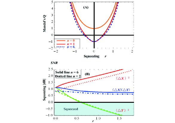
Figure 3: Nonclassical features of the ESVS. (A) The Mandel’s $Q$ parameter with fixed values of $n=0,$ $1$ and $6$. (B) Quadrature fluctuations $\left\langle\Delta X\right\rangle^{2}$ (red line), $\left\langle\Delta Y\right\rangle^{2}$ (green line) and $\left\langle\Delta X\right\rangle\cdot\left\langle\Delta Y\right\rangle$ (blue line) as the functions of the squeezing parameter $r$ with $n=2$ and $6$, respectively.

When $n=2$ and $6,$ squeezing behaviours of the ESVS have been shown in Figure 3(B). As a function of the squeezing parameter $r,$ $SNR$ is a measure to the fluctuation level that is lower than the vacuum noise. Refer to the vacuum field in units of dB, i.e. $SNR=0$ (see the black line in Figure 3(B)), $SNR<0$ means that the noise was squeezed in $Y$ quadrature. With rising the value of $r,$ $Y$ quadrature variance $\left\langle\Delta Y\right\rangle^{2}$ (green line) goes down gradually, as $X$ quadrature variance (red line) goes up and joint variance $\left\langle\Delta X\right\rangle\left\langle\Delta Y\right\rangle$ (blue line) reduces slowly. When adding more and more photons, $SNR$ has a higher level. That means squeezing behaviours of high-order ESVS can be dominated via squeezing parameter $r.$

3 Non-Gaussianity of the ESVS

The criteria and estimation for the quantum non-Gaussianity have proposed by Genoni in Refs.[41]. The non-Gaussianity can be evaluated by

$$\delta\left[\rho\right]=\frac{D_{HS}^{2}\left[\rho,\tau\right]}{\text{Tr}\left[\rho^{2}\right]}=\frac{\text{Tr}\left[\rho^{2}\right]+\text{Tr}\left[\tau^{2}\right]-2\text{Tr}\left[\rho\tau\right]}{2\text{Tr}\left[\rho^{2}\right]}=\frac{\mu\left[\rho\right]+\mu\left[\tau\right]-2\kappa\left[\rho,\tau\right]}{2\mu\left[\rho\right]},$$ (30)

in which $D_{HS}^{2}\left[\rho,\tau\right]$ is the Hilbert-Schmidt distance between the estimated state $\rho$ and the reference Gaussian state $\tau$, $\mu\left[\rho\right]\equiv$Tr$\left[\rho^{2}\right],$ $\mu\left[\tau\right]\equiv$Tr$\left[\tau^{2}\right]$, $\kappa\left[\rho,\tau\right]\equiv$Tr$\left[\rho\tau\right]$. In general, the reference Gaussian state is a displaced squeezed thermal state $\tau=D\left(\epsilon\right)S\left(\varsigma\right)\nu\left(n_{t}\right)S^{-1}\left(\varsigma\right)D^{-1}\left(\epsilon\right)$, where $D\left(\epsilon\right)=\exp\left(\epsilon a^{{\dagger}}-\epsilon^{\ast}a\right)$ and $S\left(\varsigma\right)=\exp\left[\frac{\varsigma}{2}\left(a^{{\dagger}2}-a^{2}\right)\right]$ are the displacement and squeezing operators, repectively. $\nu\left(\bar{n}\right)=\left(1+\bar{n}\right)^{-1}\left[\frac{\bar{n}}{1+\bar{n}}\right]^{a^{{\dagger}}a}=\sum_{m=0}^{\infty}\frac{\bar{n}^{m}}{\left(1+\bar{n}\right)^{m+1}}\left|m\right\rangle\left\langle m\right|$ is the thermal state with an $\bar{n}$ average number of photons. The parameters $\epsilon,$ $\varsigma$ and $\bar{n}$ are analytical functions of $n$ and $r.$ Firstly, the reference Gaussian state $\tau$ will only work if

$$X\left[\rho\right]=X\left[\tau\right],\text{ \ \ }\sigma\left[\rho\right]=\sigma\left[\tau\right],$$ (31)

in other words, their vector of mean values and the covariance matrix are equal. In (31), $X_{j}$ and $\sigma_{kj}$ denote the vector of mean values and the covariance matrix of a quantum state, respectively, satisfying

$$X_{j}=\left\langle R_{j}\right\rangle,\text{ \ \ }\sigma_{kj}=\left\langle\left\{R_{k},R_{j}\right\}\right\rangle-\left\langle R_{k}\right\rangle\left\langle R_{j}\right\rangle,$$ (32)

where the real vector $R=\left(q_{1},p_{1},q_{2},p_{2},\cdots,q_{n},p_{n}\right)^{T}\$has the commutation relations $\left[R_{k},R_{j}\right]=i\Omega_{kj},$ symbol $\left\{\cdots,\cdots\right\}$ denotes the anticommutator, $\left\langle\cdots\right\rangle$ is the expectation value, and $\Omega_{kj}$ is the elements of the symplectic matrix $\Omega=i\oplus_{k=1}^{n}\sigma_{2},$ $\sigma_{2}$ being the $y-$ Pauli matrix. From the first equation of (31), we have

$$\text{Tr}\left[a\rho\left(r,n\right)\right]=\text{Tr}\left[a\tau\left(\epsilon,\varsigma,\bar{n}\right)\right],\text{ \ \ Tr}\left[a^{{\dagger}}\rho\left(r,n\right)\right]=\text{Tr}\left[a^{{\dagger}}\tau\left(\epsilon,\varsigma,\bar{n}\right)\right],$$ (33)

and considering

$$D\left(\epsilon\right)aD^{-1}\left(\epsilon\right)=a-\epsilon,\text{ \ \ \ }D\left(\epsilon\right)a^{{\dagger}}D^{-1}\left(\epsilon\right)=a^{{\dagger}}-\epsilon^{\ast},$$ (34)

we obtain

$$\text{Tr}\left[a\tau\left(\epsilon,\varsigma,\bar{n}\right)\right]=\text{Tr}\left[a\sum_{m=0}^{\infty}\frac{\bar{n}^{m}}{\left(1+\bar{n}\right)^{m+1}}D\left(\epsilon\right)S\left(\varsigma\right)\left|m\right\rangle\left\langle m\right|S^{-1}\left(\varsigma\right)D^{-1}\left(\epsilon\right)\right]=\epsilon=\text{Tr}\left[a\rho\left(r,n\right)\right]=0.$$ (35)

Indeed, the reference Gaussian state of the ESVS is a squeezed thermal state

$$\tau\left(\varsigma,\bar{n}\right)=S\left(\varsigma\right)\nu\left(\bar{n}\right)S^{-1}\left(\varsigma\right)=\sum_{m=0}^{\infty}\frac{\bar{n}^{m}}{\left(1+\bar{n}\right)^{m+1}}S\left(\varsigma\right)\left|m\right\rangle\left\langle m\right|S^{-1}\left(\varsigma\right),$$ (36)

where the squeezing coefficient $\varsigma$ and average photons number $\bar{n}$ shall be decided by the second equation of (31), i.e.

$$\text{Tr}\left[a^{2}\rho\left(r,n\right)\right] = \text{Tr}\left[a^{2}\tau\left(\epsilon,\varsigma,\bar{n}\right)\right],\text{ \ \ }$$

$$\text{Tr}\left[a^{{\dagger}2}\rho\left(r,n\right)\right] = \text{Tr}\left[a^{{\dagger}2}\tau\left(\epsilon,\varsigma,\bar{n}\right)\right],\ \ \ \$$ (37)

$$\text{Tr}\left[a^{{\dagger}}a\rho\left(r,n\right)\right] = \text{Tr}\left[a^{{\dagger}}a\tau\left(\epsilon,\varsigma,\bar{n}\right)\right].$$

Substituting Eqs.(36) and (3) into Eq.(37), we have

$$\text{Tr}\left[a^{2}\tau\left(\varsigma,\bar{n}\right)\right] = \text{Tr}\left[a^{{\dagger}2}\tau\left(\varsigma,\bar{n}\right)\right]=\text{Tr}\left[a^{2}\sum_{m=0}^{\infty}\frac{\bar{n}^{m}}{\left(1+\bar{n}\right)^{m+1}}S\left(\varsigma\right)\left|m\right\rangle\left\langle m\right|S^{-1}\left(\varsigma\right)\right]=\left(2\bar{n}+1\right)\sinh\varsigma\cosh\varsigma=M\left(n,r\right),$$ (38)

$$\text{Tr}\left[a^{{\dagger}}a\tau\left(\epsilon,\varsigma,\bar{n}\right)\right] = \bar{n}\cosh^{2}\varsigma+\left(\bar{n}+1\right)\sinh^{2}\varsigma=N(n,r),$$

then it follows

$$\varsigma=\frac{1}{4}\ln\left[\frac{2N\left(n,r\right)+1+2M\left(n,r\right)}{2N\left(n,r\right)+1-2M\left(n,r\right)}\right],\text{ \ \ \ \ }\bar{n}=\frac{\sqrt{\left[2N\left(n,r\right)+1\right]^{2}-4M^{2}\left(n,r\right)}-1}{2},$$ (39)

$M\left(n,r\right)$ and $N\left(n,r\right)$ are also shown in (26) and (27).

Since the ESVS is a pure state, thus $\mu\left[\rho\right]\equiv$Tr$\left[\rho^{2}\right]=$Tr$\left[\rho\right]=1,$ while the squeezed thermal states is mixture, $\mu\left[\tau\right]=Tr\left[\tau^{2}\right]=\left(1+2\bar{n}\right)^{-1}.$ Substituting (36) and (3) into $\kappa\left[\rho,\tau\right],$ we can derive

$$\kappa\left[\rho,\tau\right] = C_{n}^{-1}\sum_{m=0}^{\infty}\frac{\bar{n}^{m}}{\left(1+\bar{n}\right)^{m+1}}\left\langle 0\right|S^{-1}\left(r\right)a^{n}S\left(\varsigma\right)\left|m\right\rangle\left\langle m\right|S^{-1}\left(\varsigma\right)a^{{\dagger}}{}^{n}S\left(r\right)\left|0\right\rangle$$ (40)

$$= C_{n}^{-1}\sum_{m=0}^{\infty}\frac{\bar{n}^{m}}{\left(1+\bar{n}\right)^{m+1}}\left|\Lambda\left(r,\varsigma,m,n\right)\right|^{2},$$

where $\Lambda\left(r,\varsigma,m,n\right)=\left\langle 0\right|S^{-1}\left(r\right)a^{n}S\left(\varsigma\right)\left|m\right\rangle\$has an analytical expression, for details in Appendix C,

$$\Lambda\left(r,\varsigma,m,n\right) = \frac{1}{\sqrt{m!\cosh\left(\varsigma-r\right)}}\left(-i\sqrt{\frac{\sinh 2r}{4}}\right)^{n}\left[1+\frac{\tanh\left(\varsigma-r\right)}{\tanh r}\right]^{\frac{n}{2}}\left[\frac{\tanh\left(\varsigma-r\right)}{2}\right]^{\frac{m}{2}}$$ (41)

$$\times\sum_{k=0}^{m}\dbinom{m}{k}\frac{\left(2i\right)^{k}n!}{\left(n-k\right)!}\left[\frac{2}{\left(\tanh r+\tanh\left[\varsigma-r\right]\right)\sinh\left(2\varsigma-2r\right)}\right]^{\frac{k}{2}}H_{n-k}\left(0\right)H_{m-k}\left(0\right).$$

Finally, analytical expression of the non-Gaussianity of the ESVS can be derived as

$$\delta\left[\rho\right]=\frac{1}{2}+\frac{1}{2+4\bar{n}}-C_{n}^{-1}\sum_{m=0}^{\infty}\frac{\bar{n}^{m}}{\left(1+\bar{n}\right)^{m+1}}\left|\Lambda\left(r,\varsigma,m,n\right)\right|^{2},$$ (42)

which measures the deviation with reference to a Gaussian squeezed thermal state. $\delta\left[\rho\right]=0$ if and only if $\rho$ is a Gaussian state. This point can be confirmed in Figure 4(A) with $n=0$ (pink line). In Figure 4(A), from the bottom to the top we can see that non-Gaussianity of the ESVS can be enhanced by adding more and more photon to squeezed vacuum field. Besides added photon number, non-Gaussianity also strongly depends on the squeezing level. When $\left|r\right|\rightarrow 0,$ non-Gaussianity of the ESVS has a higher performance. Similar results can be found for the case of odd photon-addition (see Figure 4(B)).

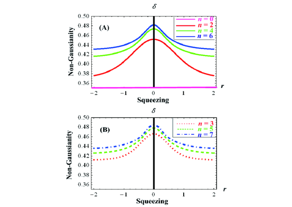
Figure 4: Non-Gaussianity of the ESVS with fixed $n$ and the varying squeezing parameter $r\in[-2,2].$ (A): Adding even photon $n=0,$ $2,$ $4,$ $6\$correspond to the solid lines from the buttom to the top. The lowest line means that non-Gaussianity of a Gaussian state is always zero (pink line). (B): Adding odd photon $n=3,$ $5,$ $7\$correspond to the dotted line, dashed line and dot-dashed line, respectively.

4 Fidelity Between the ESVS and the Photon-subtraction Squeezed Vacuum State (PSSVS)

Eq.(1) indicates that the squeezed field is an approximation of all even number photon superposition states. If adding one single photon to this squeezed field, we can simplify $a^{{\dagger}}S\left(r\right)\left|0\right\rangle\rightarrow\alpha_{1}\left|1\right\rangle+\beta_{1}\left|3\right\rangle+\gamma_{1}\left|5\right\rangle+\cdots,$ which is a superposition of odd number photon states shown in Eq.(2). When subtracting one single photon from the squeezed field, we can see

$$aS\left(r\right)\left|0\right\rangle\rightarrow\sum_{n=0}\frac{\sqrt{\left(2n-1\right)!}}{2^{n-1}\left(n-1\right)!}\tanh^{n}r\left|2n-1\right\rangle\rightarrow\alpha_{2}\left|1\right\rangle+\beta_{2}\left|3\right\rangle+\gamma_{2}\left|5\right\rangle+\cdots,$$ (43)

where $\alpha_{j},$ $\beta_{j}$ and $\gamma_{j}\ \left(j=1,2\right)$ are real. Therefore, from the point of view of the photon number distribution, the ESVS is close to the PSSVS. The similarity of these states can be estimated by difining the fidelity $F,$ i.e.

$$F=\frac{Tr\left[\rho_{0}\rho\left(r,n\right)\right]}{Tr\left[\rho_{0}^{2}\right]},$$ (44)

where $\rho\left(r,n\right)$ is the ESVS shown in Eq.(3), $\rho_{0}$ denotes the PSSVS,

$$\rho_{0}=C_{m}^{-1}a^{m}S\left(\lambda\right)\left|0\right\rangle\left\langle 0\right|S^{-1}\left(\lambda\right)a^{{\dagger}}{}^{m},$$ (45)

$C_{m}=m!\left(i\sinh\lambda\right)^{m}P_{m}\left(-i\sinh\lambda\right)$ is the normalized constant. Noting $Tr\left[\rho_{0}^{2}\right]=Tr\left[\rho_{0}\right]=1,$ we have

$$F = Tr\left[\rho_{0}\rho\left(r,n\right)\right]=Tr\left[C_{n}^{-1}C_{m}^{-1}a^{m}S\left(\lambda\right)\left|0\right\rangle\left\langle 0\right|S^{-1}\left(\lambda\right)a^{{\dagger}}{}^{m}a^{{\dagger}}{}^{n}S\left(r\right)\left|0\right\rangle\left\langle 0\right|S^{-1}\left(r\right)a^{n}\right]$$

$$= C_{n}^{-1}C_{m}^{-1}\left\langle 0\right|S^{-1}\left(r\right)a^{m+n}S\left(\lambda\right)\left|0\right\rangle\left\langle 0\right|S^{-1}\left(\lambda\right)a^{{\dagger}}{}^{m+n}S\left(r\right)\left|0\right\rangle$$

$$\equiv C_{n}^{-1}C_{m}^{-1}\left|\Gamma\left(r,\lambda,m,n\right)\right|^{2}$$

where $\Gamma\left(r,\lambda,m,n\right)=\left\langle 0\right|S^{-1}\left(r\right)a^{m+n}S\left(\lambda\right)\left|0\right\rangle.$ Comparing $\Gamma\left(r,\lambda,m,n\right)$ and $\Lambda\left(r,\varsigma,m,n\right)=\left\langle 0\right|S^{-1}\left(r\right)a^{n}S\left(\varsigma\right)\left|m\right\rangle$ shown in Eq.(40), we can obtain the analytical expression of $\Gamma\left(r,\lambda,m,n\right)$ via the replacement of $\varsigma\rightarrow\lambda,$ $m\rightarrow 0,$ and $n\rightarrow m+n$ in Eq.(41), i.e.

$$\Gamma\left(r,\lambda,m,n\right)=\frac{1}{\sqrt{\cosh\left(\lambda-r\right)}}\left(-i\sqrt{\frac{\sinh 2\lambda}{4}}\right)^{m+n}\left[1+\frac{\tanh\left(\lambda-r\right)}{\tanh r}\right]^{\frac{m+n}{2}}H_{m+n}\left[0\right].$$ (47)

As a result, the fidelity can be derived as

$$F=C_{n}^{-1}C_{m}^{-1}\frac{1}{\cosh\left(\lambda-r\right)}\left(\frac{\sinh 2r}{4}\right)^{m+n}\left[1+\frac{\tanh\left(\lambda-r\right)}{\tanh r}\right]^{m+n}\left[H_{m+n}\left(0\right)\right]^{2},$$ (48)

which is an analytical expression for the fidelity between the ESVS and the PSSVS with variance of parameters $n$, $m$, $\lambda$ and $r.$ On the left column of Figure 5 (see Figure 5(A)—5(C)), the values of photon-addition number $n$ and photon-subtraction number $m$ are independent. In Figure 5(A), taking $n=m=2,$ the fidelity as a function of the squeezing parameter $r$ can be obtianed by taking different values of $\lambda=0.2,$ $0.5,$ $1.0$ and $1.5,$ respectively. When $\lambda=1.5,$ the optimal fidelity is $0.992613$ at $r=1.4758.$ If taking $n=2,$ $m=4,$ the fidelity has been shown in Figure 5(B), and under the same conditions ($\lambda=1.5$) the optimal fidelity is $0.971793$ at $r=1.76518.$ Figure 5(C) describes the case of $n=2,$ $m=6.$

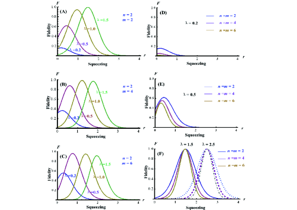
Figure 5: Fidelity between the ESVS and PSSVS with variance of parameters $n$, $m$, $\lambda$ and $r.$ With fixed values of $\lambda=0.2,$ $0.5,$ $1.0$ and $1.5,$ the left column of Figure 5 exhibits the continuously varying fidelity with (A) $n=m=2$, (B) $n=2,$ $m=4$, (C) $n=2,$ $m=6$. For the case of the same values of $n=m=2,$ $4$ and $6,$ the right column exhibits the fidelity with different squeezing (D) $\lambda=0.2$, (E) $\lambda=0.4$, (F) $\lambda=1.5$ and $2.5$.

If always taking the same values of $n$ and $m,$ the fidelity is a continuously varying with the squeezing $r$ and $\lambda$ (with the different values of $\lambda=0.2,$ $0.5,$ $1.5$ and $2.5).$ The details can be found in Figure 5(D)–5(E). With the increase of $\lambda,$ the optimal fidelity for $r$ will be pretty close to $1$. For example of $n=m=2$ and $\lambda=2.5,$ the optimal fidelity is $0.99987$ at $r=2.49645.$ When $n=4,$ $m=6,$ and taking the different values of $\lambda$ and $r$, the fidelity distribution has been shown in Figure 6(A). Figure 6(B) depicts the contour of fidelity with respect to $\lambda$ and $r.$

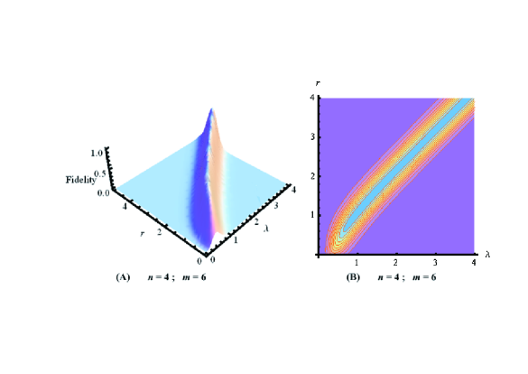
Figure 6: Fidelity distribution (A) and its contour (B) with $n=4$ and $m=6.$ As a function of the squeezing parameters $\lambda$ and $r,$ the optimal fidelity can be decided by adjusting parameters for different cases. In Figure 6(A), the ridge is the descrption of optimal fidelity. In Figure 6(B), the smaller blue region means much higher fidelity.

5 Conclusions and Remarks

Non-Gaussian operations and non-Gaussian quantum states have been proved to be very effective means and useful resources in continuous variable (CV) quantum information processes (QIP). In this work, we have introduced the excited squeezed vacuum state (ESVS), which can be ustilized to describe quantum light field emitted from multiphoton quantum process occurred in some restricted quantum systems. And then we have exhibited its nonclassical properities (e.g. the phase space Wigner distribution, photo number distributions, the second-order autocorrelation Mandel’s $Q$ parameter, the quadrature fluctuations). We have also investigated how to quantify the non-Gaussianity of the ESVS. After all, with enhanced non-Gaussian properties may constitute powerful resources for many quantum information tasks [5, 47, 2, 8, 3]. Due to the similar photon number distribution, we have examined the fidelity between the ESVS and the PSSVS, and obtianed an analytical expression of fidelity, from which the optimal fidelity can be decided by monitoring the relevant parameters. With current technology of experimental study, high fidelity preparation of the ESVS can be replaced by the PSSVS generation. In fact, the photon-subtraction operation is relatively easy to implement via the simple optical devices (e.g. beamsplitter) and coincidence measurement.

6 Acknowledgements

This work has been supported in part by the Natural Science Foundation of China (No. 61203061, 11204004, 61374091, 61403362, and 61473199), Outstanding Young Talent Foundation of Anhui Province Colleges and Universities No.2012SQRL040, and also Natural Science Foundation of Anhui Province Colleges & Universities under grant KJ2012Z035. The authors acknowledge fruitful discussions about physics meaning with Prof. Guoyong Xiang, Prof. Chaoyang Lu and their group members.

7 Appendix A: Derivation of Eq.(11)

Noting the following transformations

$$S^{-1}\left(r\right)aS\left(r\right) = a\cosh r+a^{{\dagger}}\sinh r,$$

$$S^{-1}\left(r\right)a^{{\dagger}}S\left(r\right) = a^{{\dagger}}\cosh r+a\sinh r,$$ (49)

we have

$$\rho\left(\lambda,n\right) = C_{n}^{-1}a^{{\dagger}}{}^{n}S\left(\lambda\right)\left|0\right\rangle\left\langle 0\right|S^{-1}\left(\lambda\right)a^{n}$$ (50)

$$= C_{n}^{-1}S\left(\lambda\right)\left(a^{{\dagger}}\cosh r+a\sinh r\right)^{n}\left|0\right\rangle\left\langle 0\right|\left(a\cosh r+a^{{\dagger}}\sinh r\right)^{n}S^{-1}\left(\lambda\right).$$

Thus the Wigner function of $\rho\left(\lambda,n\right)$ can be written as

$$W\left(\alpha,\alpha^{\ast}\right) = Tr\left[\rho\left(\lambda,n\right)\Delta\left(\alpha,\alpha^{\ast}\right)\right]=C_{n}^{-1}\left\langle 0\right|S^{-1}\left(\lambda\right)a^{n}\Delta\left(\alpha,\alpha^{\ast}\right)a^{{\dagger}}{}^{n}S\left(\lambda\right)\left|0\right\rangle$$ (51)

$$= C_{n}^{-1}\left\langle 0\right|\left(a\cosh r+a^{{\dagger}}\sinh r\right)^{n}S^{-1}\left(\lambda\right)\Delta\left(\alpha,\alpha^{\ast}\right)S\left(\lambda\right)\left(a^{{\dagger}}\cosh r+a\sinh r\right)^{n}\left|0\right\rangle.$$

Considering (9) and directly using the transform in (10), we have

$$S^{-1}\left(\lambda\right)\Delta\left(\alpha,\alpha^{\ast}\right)S\left(\lambda\right) = \frac{1}{2}S^{-1}\left(\lambda\right)\begin{array}[]{c}\dot{\vdots}\end{array}\delta\left(a-\alpha\right)\delta\left(a^{\dagger}-\alpha^{\ast}\right)\begin{array}[]{c}\dot{\vdots}\end{array}S\left(\lambda\right)$$ (54)

$$= \frac{1}{2}\begin{array}[]{c}\dot{\vdots}\end{array}\delta\left(a\cosh r+a^{{\dagger}}\sinh r-\alpha\right)\delta\left(a^{{\dagger}}\cosh r+a\sinh r-\alpha^{\ast}\right)\begin{array}[]{c}\dot{\vdots}\end{array}$$ (57)

$$= \frac{1}{2}\begin{array}[]{c}\dot{\vdots}\end{array}\delta\left(a-\alpha\cosh r+\alpha^{\ast}\sinh r\right)\delta\left(a^{{\dagger}}-\alpha^{\ast}\cosh r+\alpha\sinh r\right)\begin{array}[]{c}\dot{\vdots}\end{array}.$$ (60)

The first equation of Eq.(9) indicates

$$S^{-1}\left(\lambda\right)\Delta\left(\alpha,\alpha^{\ast}\right)S\left(\lambda\right)\rightarrow\Delta\left(z,z^{\ast}\right)=\int\frac{d^{2}\beta}{\pi^{2}}\left|z+\beta\right\rangle\left\langle z-\beta\right|e^{z\beta^{\ast}-z^{\ast}\beta},$$ (61)

where $z=\alpha\cosh r-\alpha^{\ast}\sinh r.$ Thus we have

$$W\left(\alpha,\alpha^{\ast}\right)=C_{n}^{-1}\left\langle 0\right|\left(a\cosh r+a^{{\dagger}}\sinh r\right)^{n}\int\frac{d^{2}\beta}{\pi^{2}}\left|z+\beta\right\rangle\left\langle z-\beta\right|e^{z\beta^{\ast}-z^{\ast}\beta}\left(a^{{\dagger}}\cosh r+a\sinh r\right)^{n}\left|0\right\rangle.$$ (62)

Ref. [40] has given a formular

$$\left(fa+ga^{{\dagger}}\right)^{n}=\left(-i\sqrt{\frac{fg}{2}}\right)^{n}\colon H_{n}\left(i\sqrt{\frac{f}{2g}}a+i\sqrt{\frac{g}{2f}}a^{{\dagger}}\right)\colon,$$ (63)

then it follows

$$\left(a^{{\dagger}}\cosh r+a\sinh r\right)^{n} = \left(-i\sqrt{\frac{\sinh 2r}{4}}\right)^{n}\colon H_{n}\left(i\sqrt{\frac{\sinh r}{2\cosh r}}a+i\sqrt{\frac{\cosh r}{2\sinh r}}a^{{\dagger}}\right)\colon,$$

$$\left(a\cosh r+a^{{\dagger}}\sinh r\right)^{n} = \left(-i\sqrt{\frac{\sinh 2r}{4}}\right)^{n}\colon H_{n}\left(i\sqrt{\frac{\cosh r}{2\sinh r}}a+i\sqrt{\frac{\sinh r}{2\cosh r}}a^{{\dagger}}\right)\colon.$$ (64)

Substituting (64) into (62), we can see

$$W\left(\alpha,\alpha^{\ast}\right) = C_{n}^{-1}\left(-\frac{\sinh 2r}{4}\right)^{n}\int\frac{d^{2}\beta}{\pi^{2}}H_{n}\left[i\sqrt{\frac{\cosh r}{2\sinh r}}\left(z+\beta\right)\right]H_{n}\left[i\sqrt{\frac{\cosh r}{2\sinh r}}\left(z^{\ast}-\beta^{\ast}\right)\right]$$

$$\times\exp\left[-\left|z\right|^{2}-\left|\beta\right|^{2}+z\beta^{\ast}-z^{\ast}\beta\right].$$

Recall the generating function of the Hermite polynomials

$$H_{n}\left(x\right)=\frac{\partial{}^{n}}{\partial t{}^{n}}\left.\exp\left(2xt-t^{2}\right)\right|_{t=0},$$ (66)

we have

$$W\left(\alpha,\alpha^{\ast}\right) = C_{n}^{-1}\left(-\frac{\sinh 2r}{4}\right)^{n}\frac{\partial{}^{2n}}{\partial t{}^{n}\partial\tau{}^{n}}\int\frac{d^{2}\beta}{\pi^{2}}\exp\left[-\left|z\right|^{2}-\left|\beta\right|^{2}+z\beta^{\ast}-z^{\ast}\beta\right]$$ (67)

$$\times\left.\exp\left[2i\sqrt{\frac{\cosh r}{2\sinh r}}\left(z+\beta\right)t-t^{2}+2i\sqrt{\frac{\cosh r}{2\sinh r}}\left(z^{\ast}-\beta^{\ast}\right)\tau-\tau^{2}\right]\right|_{t,\tau=0},$$

and noting the following integral formula

$$\int\frac{d^{2}\alpha}{\pi}\exp\left[h\left|\alpha\right|^{2}+s\alpha+\eta\alpha^{\ast}+f\alpha^{2}+g\alpha^{\ast 2}\right]=\frac{1}{\sqrt{h^{2}-4fg}}\exp\left[\frac{-hs\eta+s^{2}g+\eta^{2}f}{h^{2}-4fg}\right],$$ (68)

whose convergent condition is Re$\left[h\pm f\pm g\right]<0$ and Re$\left[\frac{h^{2}-4fg}{h\pm f\pm g}\right]<0,$ we can derive

$$W\left(\alpha,\alpha^{\ast}\right) = C_{n}^{-1}\left(-\frac{\sinh 2r}{4}\right)^{n}\exp\left[-2\left|z\right|^{2}\right]$$ (69)

$$\times\left.\frac{\partial{}^{2n}}{\partial t{}^{n}\partial\tau{}^{n}}\exp\left[-t^{2}-\tau^{2}+4i\sqrt{\frac{\cosh r}{2\sinh r}}zt+4i\sqrt{\frac{\cosh r}{2\sinh r}}z^{\ast}\tau+\frac{2\cosh r}{\sinh r}t\tau\right]\right|_{t,\tau=0}.$$

Using Eq.(66) again, we have

$$W\left(\alpha,\alpha^{\ast}\right) = C_{n}^{-1}\left(-\frac{\sinh 2r}{4}\right)^{n}\exp\left[-2\left|z\right|^{2}\right]$$

$$\times\left.\frac{\partial{}^{n}}{\partial t{}^{n}}\left\{\left[H_{n}\left(2i\sqrt{\frac{\cosh r}{2\sinh r}}z^{\ast}+\frac{\cosh r}{\sinh r}t\right)\right]\exp\left[-t^{2}+4i\sqrt{\frac{\cosh r}{2\sinh r}}zt\right]\right\}\right|_{t=0},$$

then it follows

$$W\left(\alpha,\alpha^{\ast}\right) = C_{n}^{-1}\left(-\frac{\sinh 2r}{4}\right)^{n}\exp\left[-2\left|z\right|^{2}\right]\sum_{m=0}^{n}\dbinom{n}{m}$$ (71)

$$\times\left.\frac{\partial^{m}}{\partial t^{m}}H_{n}\left(i\sqrt{\frac{2}{\tanh r}}z^{\ast}+\frac{t}{\tanh r}\right)\times\frac{\partial^{n-m}}{\partial t^{n-m}}\exp\left[-t^{2}+2i\sqrt{\frac{2}{\tanh r}}zt\right]\right|_{t=0}.$$

By virtue of the recurrence relation of $H_{n}\left(x\right)$

$$\frac{d^{l}}{dx^{l}}H_{n}\left(x\right)=\frac{2^{l}n!}{\left(n-l\right)!}H_{n-l}\left(x\right),$$ (72)

we have

$$W\left(\alpha,\alpha^{\ast}\right)=C_{n}^{-1}\left(\frac{\sinh 2r}{4}\right)^{n}\exp\left(-2\left|z\right|^{2}\right)\sum_{m=0}^{n}\dbinom{n}{m}\frac{2^{m}n!}{\left(n-m\right)!}\left(-\coth r\right)^{m}\left|H_{n-m}\left(-i\sqrt{\frac{2}{\tanh r}}z\right)\right|^{2}$$ (73)

and substituting $z=\alpha\cosh r-\alpha^{\ast}\sinh r$ into the above equation, finally we obtain the Wigner function of the ESVS

$$W\left(\alpha,\alpha^{\ast}\right) = \frac{1}{P_{n}\left(\cosh r\right)}\left(\frac{\sinh r}{2}\right)^{n}\exp\left[-2\left|\alpha\cosh r-\alpha^{\ast}\sinh r\right|^{2}\right]$$ (74)

$$\times\sum_{m=0}^{n}\dbinom{n}{m}\frac{2^{m}n!}{\left(n-m\right)!}\left(-\coth r\right)^{m}\left|H_{n-m}\left[-i\sqrt{\frac{2}{\tanh r}}\left(\alpha\cosh r-\alpha^{\ast}\sinh r\right)\right]\right|^{2}.$$

8 Appendix B: Derivation of Expected Value in Eq.(24)

From (63), we have

$$\left(a^{{\dagger}}\cosh r+a\sinh r\right)^{n+l} = \left(-i\sqrt{\frac{\sinh r\cosh r}{2}}\right)^{n+l}\colon H_{n+l}\left(i\sqrt{\frac{\sinh r}{2\cosh r}}a+i\sqrt{\frac{\cosh r}{2\sinh r}}a^{{\dagger}}\right)\colon,$$

$$\left(a\cosh r+a^{{\dagger}}\sinh r\right)^{n+k} = \left(-i\sqrt{\frac{\sinh r\cosh r}{2}}\right)^{n+k}\colon H_{n+k}\left(i\sqrt{\frac{\cosh r}{2\sinh r}}a+i\sqrt{\frac{\sinh r}{2\cosh r}}a^{{\dagger}}\right)\colon.$$ (75)

Inserting the completeness $\pi^{-1}\int d^{2}\beta\left|\beta\right\rangle\left\langle\beta\right|=1$ of coherent state $\left|\beta\right\rangle$ into (23), we have

$$\left\langle\lambda,n\right|a^{k}a^{{\dagger}}{}^{l}\left|\lambda,n\right\rangle = C_{n}^{-1}\left(-i\sqrt{\frac{\sinh 2r}{4}}\right)^{k}\left(-i\sqrt{\frac{\sinh 2r}{4}}\right)^{l}\left(-\frac{\sinh 2r}{4}\right)^{n}$$ (76)

$$\times\int\frac{d^{2}\beta}{\pi^{2}}H_{n+k}\left(i\sqrt{\frac{\cosh r}{2\sinh r}}\beta\right)H_{n+l}\left(i\sqrt{\frac{\cosh r}{2\sinh r}}\beta^{\ast}\right)\exp\left(-\left|\beta\right|^{2}\right).$$

Using Eq.(66) twice, we have

$$\left\langle\lambda,n\right|a^{k}a^{{\dagger}}{}^{l}\left|\lambda,n\right\rangle = C_{n}^{-1}\left(-i\sqrt{\frac{\sinh 2r}{4}}\right)^{k}\left(-i\sqrt{\frac{\sinh 2r}{4}}\right)^{l}\left(-\frac{\sinh 2r}{4}\right)^{n}\frac{\partial{}^{n+k}}{\partial t{}^{n+k}}\frac{\partial{}^{n+l}}{\partial\tau{}^{n+l}}$$ (77)

$$\times\left.\int\frac{d^{2}\beta}{\pi^{2}}\exp\left[-\left|\beta\right|^{2}-t^{2}+2i\sqrt{\frac{\cosh r}{2\sinh r}}\beta t-\tau^{2}+2i\sqrt{\frac{\cosh r}{2\sinh r}}\beta^{\ast}\tau\right]\right|_{t,\tau=0},$$

and using the following integral formula

$$\int\frac{d^{2}\alpha}{\pi}\exp\left[h\left|\alpha\right|^{2}+s\alpha+\eta\alpha^{\ast}\right]=\frac{1}{h}\exp\left[-\frac{s\eta}{h}\right],\text{ \ Re}\left[h\right]<0,$$

we can obtain

$$\left\langle\lambda,n\right|a^{k}a^{{\dagger}}{}^{l}\left|\lambda,n\right\rangle = C_{n}^{-1}\left(-i\sqrt{\frac{\sinh 2r}{4}}\right)^{k}\left(-i\sqrt{\frac{\sinh 2r}{4}}\right)^{l}\left(-\frac{\sinh 2r}{4}\right)^{n}\left.\frac{\partial{}^{n+k}}{\partial t{}^{n+k}}\frac{\partial{}^{n+l}}{\partial\tau{}^{n+l}}\exp\left[-t^{2}-\tau^{2}-2\frac{\cosh r}{\sinh r}t\tau\right]\right|_{t,\tau=0}$$

$$= C_{n}^{-1}\left(-i\sqrt{\frac{\sinh 2r}{4}}\right)^{k}\left(i\sqrt{\frac{\sinh 2r}{4}}\right)^{l}\left(\frac{\sinh 2r}{4}\right)^{n}\left.\frac{\partial{}^{n+k}}{\partial t{}^{n+k}}\left[H_{n+l}\left(\frac{\cosh r}{\sinh r}t\right)\exp\left[-t^{2}\right]\right]\right|_{t=0}$$

$$= C_{n}^{-1}\left(-i\sqrt{\frac{\sinh 2r}{4}}\right)^{k}\left(i\sqrt{\frac{\sinh 2r}{4}}\right)^{l}\left(\frac{\sinh 2r}{4}\right)^{n}$$

$$\times\sum_{m=0}^{n+k}\dbinom{n+k}{m}\coth^{m}r\times\left[\frac{\partial^{m}}{\partial t^{m}}H_{n+l}\left(t\right)\right]\times\left.\frac{\partial^{n+k-m}}{\partial t^{n+k-m}}\exp\left(-t^{2}\right)\right|_{t=0}.$$

Then using the recurrence relation in (72) and the differential form of the Hermite polynomials in Eq. (15), we can derive

$$\left\langle\lambda,n\right|a^{k}a^{{\dagger}}{}^{l}\left|\lambda,n\right\rangle = C_{n}^{-1}\left(-i\sqrt{\frac{\sinh 2r}{4}}\right)^{k}\left(i\sqrt{\frac{\sinh 2r}{4}}\right)^{l}\left(\frac{\sinh 2r}{4}\right)^{n}$$ (79)

$$\times\sum_{m=0}^{n+k}\dbinom{n+k}{m}\frac{\left(-1\right)^{n+k-m}2^{m}\left(n+l\right)!\coth^{m}r}{\left(n+l-m\right)!}H_{n+l-m}\left(0\right)H_{n+k-m}\left(0\right).$$

9 Appendix C: Derivation of Non-Gaussianity in Eq.(41)

Noting Eqs.(49), (63) and (64), we have

$$\Lambda\left(r,\varsigma,m,n\right) \equiv \left\langle 0\right|S^{-1}\left(r\right)a^{n}S\left(\varsigma\right)\left|m\right\rangle=\left\langle 0\right|\left(a\cosh r+a^{{\dagger}}\sinh r\right)^{n}S\left(\varsigma-r\right)\left|m\right\rangle$$ (80)

$$= \left(-i\sqrt{\frac{\sinh r\cosh r}{2}}\right)^{n}\left\langle 0\right|H_{n}\left(i\sqrt{\frac{\cosh r}{2\sinh r}}a\right)S\left(\nu\right)\left|m\right\rangle,$$

where $\nu=\varsigma-r.$ Inserting the completeness relation of coherent state into the above equation and using $\left|m\right\rangle=\left.\frac{1}{\sqrt{m!}}\frac{d^{m}}{d\alpha^{m}}\left|\alpha\right\rangle\right|_{\alpha=0}$ ($\left|\alpha\right\rangle=\exp\left(\alpha a^{{\dagger}}\right)\left|0\right\rangle$), we have

$$\Lambda\left(r,\varsigma,m,n\right) = \frac{1}{\sqrt{m!}}\left(-i\sqrt{\frac{\sinh r\cosh r}{2}}\right)^{n}\left.\frac{d^{m}}{d\alpha^{m}}\left\langle 0\right|H_{n}\left(i\sqrt{\frac{\cosh r}{2\sinh r}}a\right)\int\frac{d^{2}z}{\pi}\left|z\right\rangle\left\langle z\right|S\left(\nu\right)\left|\alpha\right\rangle\right|_{\alpha=0}$$

$$= \frac{1}{\sqrt{m!\cosh\nu}}\left(-i\sqrt{\frac{\sinh r\cosh r}{2}}\right)^{n}\left.\frac{d^{m}}{d\alpha^{m}}\exp\left(-\frac{\tanh\nu}{2}\alpha^{2}\right)\right.$$

$$\times\left.\int\frac{d^{2}z}{\pi}H_{n}\left(i\sqrt{\frac{\cosh r}{2\sinh r}}z\right)\exp\left[-\left|z\right|^{2}+\frac{\tanh\nu}{2}z^{\ast 2}+z^{\ast}\alpha\sec h\nu\right]\right|_{\alpha=0},$$

from (66), then it follows

$$\Lambda\left(r,\varsigma,m,n\right) = \frac{1}{\sqrt{m!\cosh\nu}}\left(-i\sqrt{\frac{\sinh r\cosh r}{2}}\right)^{n}\left.\frac{d^{m}}{d\alpha^{m}}\exp\left(-\frac{\tanh\nu}{2}\alpha^{2}\right)\right.$$ (82)

$$\times\left.\frac{\partial{}^{n}}{\partial t{}^{n}}\exp\left(-t^{2}\right)\int\frac{d^{2}z}{\pi}\left.\exp\left(-\left|z\right|^{2}+\frac{\tanh\nu}{2}z^{\ast 2}+z^{\ast}\alpha\sec h\nu+2i\sqrt{\frac{\cosh r}{2\sinh r}}zt\right)\right|_{t=0}\right|_{\alpha=0}.$$

Thus Eq.(68) can tell us

$$\Lambda\left(r,\varsigma,m,n\right) = \frac{1}{\sqrt{m!\cosh\nu}}\left(-i\sqrt{\frac{\sinh r\cosh r}{2}}\right)^{n}\left.\frac{d^{m}}{d\alpha^{m}}\exp\left(-\frac{\tanh\nu}{2}\alpha^{2}\right)\right.$$ (83)

$$\times\left.\left.\frac{\partial{}^{n}}{\partial t{}^{n}}\exp\left[-\left(1+\frac{\tanh\nu}{\tanh r}\right)t^{2}+it\alpha\sqrt{\frac{2\cosh r}{\sinh r}}\sec h\nu\right]\right|_{t=0}\right|_{\alpha=0}.$$

Using (66) again, we can see

$$\Lambda\left(r,\varsigma,m,n\right) = \frac{1}{\sqrt{m!\cosh\nu}}\left(-i\sqrt{\frac{\sinh r\cosh r}{2}}\right)^{n}\left(1+\frac{\tanh\nu}{\tanh r}\right)^{\frac{n}{2}}$$ (84)

$$\times\left.\frac{d^{m}}{d\alpha^{m}}H_{n}\left(\frac{i\alpha\sec h\nu}{\sqrt{2\left(\tanh r+\tanh\nu\right)}}\right)\exp\left(-\frac{\tanh\nu}{2}\alpha^{2}\right)\right|_{\alpha=0},$$

then it follows

$$\Lambda\left(r,\varsigma,m,n\right) = \frac{1}{\sqrt{m!\cosh\nu}}\left(-i\sqrt{\frac{\sinh r\cosh r}{2}}\right)^{n}\left(1+\frac{\tanh\nu}{\tanh r}\right)^{\frac{n}{2}}$$ (85)

$$\times\left.\sum_{k=0}^{m}\dbinom{m}{k}\frac{d^{k}}{d\alpha^{k}}H_{n}\left[\frac{i\alpha\sec h\nu}{\sqrt{2\left(\tanh r+\tanh\nu\right)}}\right]\frac{d^{m-k}}{d\alpha^{m-k}}\exp\left(-\frac{\tanh\nu}{2}\alpha^{2}\right)\right|_{\alpha=0}.$$

From (72), we have

$$\Lambda\left(r,\varsigma,m,n\right) = \frac{1}{\sqrt{m!\cosh\nu}}\left(-i\sqrt{\frac{\sinh r\cosh r}{2}}\right)^{n}\left(1+\frac{\tanh\nu}{\tanh r}\right)^{\frac{n}{2}}\sum_{k=0}^{m}\dbinom{m}{k}\frac{2^{k}n!}{\left(n-k\right)!}$$ (86)

$$\times\left(\frac{i\sec h\nu}{\sqrt{2\left(\tanh r+\tanh\nu\right)}}\right)^{k}\left.H_{n-k}\left(\frac{i\alpha\sec h\nu}{\sqrt{2\left(\tanh r+\tanh\nu\right)}}\right)\frac{d^{m-k}}{d\alpha^{m-k}}\exp\left(-\frac{\tanh\nu}{2}\alpha^{2}\right)\right|_{\alpha=0}$$

and due to $\left.\frac{d^{m-k}}{d\alpha^{m-k}}\exp\left(-\frac{\tanh\nu}{2}\alpha^{2}\right)\right|_{\alpha=0}=\left(\frac{\tanh\nu}{2}\right)^{\frac{m-k}{2}}H_{m-k}\left(0\right)$, finally we can derive

$$\Lambda\left(r,\varsigma,m,n\right) = \frac{1}{\sqrt{m!\cosh\left(\varsigma-r\right)}}\left(-i\sqrt{\frac{\sinh 2r}{4}}\right)^{n}\left[1+\frac{\tanh\left(\varsigma-r\right)}{\tanh r}\right]^{\frac{n}{2}}\left[\frac{\tanh\left(\varsigma-r\right)}{2}\right]^{\frac{m}{2}}$$ (87)

$$\times\sum_{k=0}^{m}\dbinom{m}{k}\frac{\left(2i\right)^{k}n!}{\left(n-k\right)!}\left[\frac{2}{\left(\tanh r+\tanh\left[\varsigma-r\right]\right)\sinh\left(2\varsigma-2r\right)}\right]^{\frac{k}{2}}H_{n-k}\left(0\right)H_{m-k}\left(0\right).$$

References

- [1] H. Takahashi, J. S. Neergaard-Nielsen, M. Takeuchi, M. Takeoka, K. Hayasaka, A. Furusawa, and M. Sasaki, Nature Photonics 4, 178 (2009).
- [2] R. F. Dong, M. Lassen, J. Heersink, C. Marquardt, R. Filip, G. Leuchs, and U. L. Andersen, Nature 4, 919 (2008).
- [3] G. Y. Xiang, T. C. Ralph, A. P. Lund, N. Walk, and G. J. Pryde, Nature Photonics 4, 316 (2010).
- [4] A. Gilchrist, K. Nemoto, W. J. Munro, T. C. Ralph, S. Glancy, S. L. Braunstein, and G. J. Milburn, Journal of Optics B 6, S828 (2004).
- [5] N. J. Cerf, O. Krüger, P. Navez, R. F. Werner, and M. M. Wolf, Physical Review Letters 95, 070501 (2005).
- [6] S. J. van Enk, and O. Hirota, Physical Review A 64, 022313 (2001); T. Opatrný, G. Kurizki, and D. G. Welsch, Physical Review A 61, 032302 (2000); P. T. Cochrane, T. C. Ralph, and G. J. Milburn, Physical Review A 65, 062306 (2002); S. Olivares, M. G. A. Paris, and R. Bonifacio, Physical Review A 67, 032314 (2003).
- [7] T. C. Ralph, A. Gilchrist, G. J. Milburn, W. J. Munro, and S. Glancy, Physical Review A 68, 042319 (2003).
- [8] A. P. Lund, T. C. Ralph, and H. L. Haselgrove, Physical Review Letters 100, 030503 (2008).
- [9] M. S. Kim, H. Jeong, A. Zavatta, V. Parigi, and M. Bellini, Physical Review Letters 101, 260401 (2008).
- [10] A. I. Lvovsky, and J. Mlynek, Physical Review Letters 88, 250401 (2002).
- [11] K. J. Resch, J. S. Lundeen, and A. M. Steinberg, Physical Review Letters 89, 037904 (2002).
- [12] J. S. Neergaard-Nielsen, B. M. Nielsen, C. Hettich, K. Molmer, and E. S. Polzik, Physcial Review Letters 97, 083604 (2006).
- [13] K. Wakui, H. Takahashi, A. Furusawa, and M. Sasaki, Optics Express 15, 3568 (2007).
- [14] T. J. Bartley, G. Donati, J. B. Spring, X. M. Jin, M. Barbieri, A. Datta, B. J. Smith, and I. A. Walmsley, Physical Review A 45, 5193 (2012).
- [15] X. X. Xu, H. C. Yuan, and Y. Wang, Chinese Physics B 23, 070301 (2014).
- [16] X. F. Xu, S. Wang, and B. Tang, Chinese Physics B 23, 024206 (2014).
- [17] L. Y. Hu, X. X. Xu, and H. Y. Fan, Journal of the Optical Society of America B-Optical Physics 27, 286 (2010).
- [18] V. Madhok, and A. Datta, International Journal of Modern Physics B 27, 1245041 (2013).
- [19] A. Datta, A. Shaji, and C. M. Caves, Physical Review Letters 100, 050502 (2008); A. Datta and A. Shaji, International Journal of Quantum Information 9, 1787 (2011); A. Brodutch, and D. R. Terno, Physical Review A 83, 010301 (2011); A. Al-Qasimi, and D. F. V. James, Physical Review A 83, 032101 (2011); G. Passante, O. Moussa, D. A. Trottier, and R. Laflamme, Physical Review A 84, 044302 (2011).
- [20] B. Dakić, Y. O. Lipp, X. S. Ma, M. Ringbauer, S. Kropatschek, S. Barz, T. Paterek, V. Vedral, A. Zeilinger, C. Brukner, and P. Walther, Nature Physics 8, 666 (2012).
- [21] I. Schuster, A. Kubanek, A. Fuhrmanek, T. Puppe, P. W. H. Pinkse, K. Murr, and G. Rempe, Nature physics 4, 382 (2008).
- [22] A. Majumdar, M. Bajcsy, and J. Vučković, Physical Review A 85, 041801(R) (2012).
- [23] S. Rebić, J. Twamley, and G. J Milburn, Physical Review Letters 103, 150503 (2009).
- [24] S. L. Braunstein, and A. K. Pati, Quantum Information with Continuous Variables, Kluwer Akademic Press, Dordrecht, 2003.
- [25] V. Giovannetti, S. Lloyd, and L. Maccone, Science 306, 1330 (2004).
- [26] G. Rempe, H. Walther, and N. Klein, Physical Review Letters 58, 353 (1987).
- [27] D. I. Schuster, A. A. Houck, J. A. Schreier, A. Wallraff, J. M. Gambetta, A. Blais, L. Frunzio, J. Majer, B. Johnson, M. H. Devoret, S. M. Girvin, and R. J. Schoelkopf, Nature 445, 515 (2007).
- [28] P. Maunz, T. Puppe, I. Schuster, N. Syassen, P.W. H. Pinkse, and G. rempe, Physical Review Letters 94, 033002 (2005).
- [29] D. Press, S. Götzinger, S. Reitzenstein, C. Hofmann, A. Löffler, M. Kamp, A. Forchel, and Y. Yamamoto, Physical Review Letters 98, 117402 (2007).
- [30] K. Hennessy, A. Badolato, M. Winger, D. Gerace, M. Atatüre, S. Gulde, S. Fält, E. L. Hu, and A. Imamoǧlu, Nature 445, 896–899 (2007).
- [31] H. J. Carmichael, L. Tian, W. Ren, and P. Alsing, Cavity Quantum Electrodynamics (ed. Berman, P. R.) 381–423 (Advances in Atomic, Molecular, and Optical Physics, Academic, New York, 1994)
- [32] P. R. Rice, and C. A. Baird, Physical Review A 53, 3633 (1996).
- [33] C. Cabrillo, W. S. Smyth, S. Swain, and P. Zhou, Optics Communications 114, 344 (1995).
- [34] S. Swain, and B. J. Dalton, Optics Communications 147, 187 (1998).
- [35] S. V. Lawande, and P. V. Panat, Jounal of Physics B: Atomic, Molecular and Optical Physics 37, 2577 (2004).
- [36] J. H. An, S. J. Wang, H. G. Luo, and C. L. Jia, Journal of Optics B: Quantum and Semiclassical Optics 5, 510 (2004).
- [37] J. Zhang, R. B. Wu, Y. X. Liu, C. W. Li , and T. J. Tarn IEEE Transaction on Automatic Control 57 1997-2008 (2012).
- [38] R. B. Wu, T. F. Li, A. G. Kofman, J. Zhang, Y. X. Liu, A. Pashkin, J. S. Tsai, and N. Franco, Physical Review A 87 022324 (2013).
- [39] K. W. Murch, S. J. Weber, K. M. Beck, E. Ginossar, and I. Siddiqi, Nature 499, 62 (2013).
- [40] X. G. Meng, J. S. Wang, and H. Y. Fan, Physics Letter A 361, 183 (2007).
- [41] M. G. Genoni, M. G. A. Paris, and K. Banaszek, Physical Review A 76, 042327 (2007).
- [42] H. Weyl, Zeitschrift für Physik 46, 1 (1927).
- [43] H. Y. Fan, Journal of Optics B: Quantum Semiclass. Optics 5, R1 (2003).
- [44] R. J. Glauber, Physical Review 130, 2529 (1963); 131, 2766 (1963).
- [45] H. Y. Fan, Annal of Physics (NY) 320, 480 (2006); 323, 1502 (2008).
- [46] L. Mandel, Optics Letter 4, 205 (1979).
- [47] A. Ourjoumtsev, H. Jeong, R. Tualle-Brouri, and P. Grangier, Nature 448, 784 (2007).