Searching for primordial localized features with CMB and LSS spectra
Abstract
Inspired by the study of mild transient reductions in the speed of sound of the adiabatic mode during inflation, we search for a primordial localized feature imprinted in cosmic microwave background and large-scale structure formation observables. We find some common oscillatory patterns both in the Planck CMB temperature-temperature power spectrum and the WiggleZ galaxy spectrum. By performing independent searches with these two data sets, we find a coincidence in the most significant mode previously found by Achúcarro et al. 2013 by using only Planck data. Furthermore, the joint data analysis shows that the oscillation frequency of the feature gets better constrained, and the amplitude marginally deviates from zero, unlike what was observed using only Planck data. Besides the parameter estimation, we also discuss the Bayesian evidence. The addition of WiggleZ data mildly enhances the significance of the best mode found in the Planck data.
pacs:
04.60.-m; 98.80.-k; 98.80.Cq; 98.80.QcI Introduction
There exist several hints of oscillatory signals in the cosmic microwave background (CMB) observables, such as power spectrum Bennett:2012zja ; Ade:2013uln and bispectrum Ade:2013ydc . This motivates a search for such kind of features produced by inflationary scenarios beyond canonical single-field.111By canonical single-field we mean slow-roll regime, Bunch-Davies vacuum and canonical kinetic terms, with . Several mechanisms that produce oscillatory features have been realized, such as a transient reduction in the speed of sound Achucarro:2012fd ; Achucarro:2013cva ; Achucarro:2014msa , step inflaton potential Starobinsky:1992ts ; Adams:2001vc ; Gong:2005jr ; Chen:2008wn ; Arroja:2011yu ; Martin:2011sn ; Adshead:2011jq ; Arroja:2012ae ; Bartolo:2013exa ; Cannone:2014qna ; Covi:2006ci ; Benetti:2011rp ; Benetti:2013cja ; Hamann:2007pa ; Benetti:2012wu ; Stewart:2001cd ; Choe:2004zg ; Dvorkin:2009ne ; Adshead:2011bw ; Miranda:2012rm ; Adshead:2013zfa , different initial vacuum states Danielsson:2002kx ; Greene:2004np ; Meerburg:2009ys ; Jackson:2010cw , multi-field dynamics Gao:2012uq ; Gao:2013ota ; Saito:2013aqa ; Noumi:2013cfa ; Chen:2014joa ; Chen:2012ja , or phenomenological superimposed oscillations in the primordial power spectrum Martin:2003sg ; Flauger:2009ab ; Flauger:2010ja ; Aich:2011qv ; Meerburg:2011gd ; Peiris:2013opa ; Meerburg:2013cla ; Meerburg:2013dla ; Meerburg:2014kna . In this work we focus on searching for oscillatory features in the scenario of a transient reduction in the speed of sound. The effect of a variable speed of sound has also been analyzed both in the power spectrum Achucarro:2010da ; Hu:2011vr ; Achucarro:2012fd and bispectrum Achucarro:2012fd ; Adshead:2013zfa ; Ribeiro:2012ar . Similar studies of power spectrum Park:2012rh ; Miranda:2012rm ; Nakashima:2010sa ; Bean:2008na ; Bartolo:2013exa and bispectrum Bean:2008na ; Bartolo:2013exa ; Meerburg:2010ks have also been done for models with sudden variations. In addition, the Planck collaboration searched for features in the CMB bispectrum for a number of theoretically motivated templates Ade:2013ydc , including oscillatory templates. Although in none of these cases the statistical significance of the extended models has been found to be high enough to claim a detection, with the improvement of experimental accuracy we are now at the threshold of verifying or falsifying these models.
Our test case, introduced in Achucarro:2013cva , consists of a gaussian reduction in the speed of sound occurring within the window of -folds corresponding to the angular scales probed by CMB and large-scale structure (LSS) surveys. Its functional form is consistent with a reduction in the speed of sound resulting from a soft turn along the inflationary trajectory in a multi-field theory in which the mass hierarchy is large enough to allow for an effective single-field description Achucarro:2010jv ; Achucarro:2010da ; Cespedes:2012hu ; Achucarro:2012sm (though one should keep in mind that a similar reduction in the speed of sound may result from a different high-energy completion of the effective field theory).
Since it is the same curvature perturbations that set the initial conditions for CMB anisotropies and large-scale structure distributions, the primordial oscillatory signals should be imprinted in all the observables of CMB anisotropy and LSS tracers, like CMB spectra, bispectra, galaxy spectra, etc. Based on this consideration, in this paper we search for primordial oscillatory features from a transient reduction in the speed of sound of adiabatic curvature perturbations via both CMB anisotropy temperature-temperature spectrum of the Planck satellite as well as galaxy distribution spectrum of the WiggleZ telescope. The rest of this paper is organized as follows. In Sec. II, we will briefly review the theoretical setup of the transient reductions in the speed of sound. In Sec. III, we will introduce the methodology of parameter estimation and model selection which is adopted in this work as well as the data sets used. Then, we arrive at our results and discuss them in Sec. IV. Finally, we conclude in Sec. V.
II Review of the model
In the framework of effective field theory, heavy fields coupled to the inflaton reduce the speed of sound of the adiabatic mode each time the background inflationary trajectory makes a turn. In reference Achucarro:2012fd , Achúcarro et al. prove how small but abrupt changes in the speed of sound of the adiabatic mode during inflation, independently of their physical origin, seed discriminable features in the primordial power spectrum and bispectrum.
Defining , at first order in this quantity a small transient reduction in the speed of sound produces a feature in the primordial scalar curvature power spectrum of the form
| (1) |
where is the featureless power spectrum with constant speed of sound , and is the conformal time. The corresponding feature in the primordial bispectrum can also be found in Achucarro:2012fd , and its calculation is valid in the perturbative regime of small . In the whole framework, it is assumed that the effect of the reduction in the speed of sound in both spectrum and bispectrum dominates over slow roll contributions. Both perturbativity and dominance over slow roll effects set bounds for the shape and the size of speed of sound reduction as
| (2) |
In this paper, following references Achucarro:2013cva ; Achucarro:2014msa , we search for reductions in the speed of sound which take the form of a gaussian in -folds :
| (3) |
where we have introduced the parameters of the feature: the amplitude , the sharpness , and the instant of maximal reduction (or ).222Assuming that the slow-roll regime remains uninterrupted, conformal time and the -folds time scale are related by , where is the value of the scale factor when there were -folds left until the end of inflation – we take here . Eq. (2) imposes limits on the maximum and minimum values of the first two parameters, and , while , from the theoretical point of view, lacks a lower bound. One can set more conservative bounds on those parameters by imposing that the feature falls within the observable window of inflation in the CMB , and it is at the same time sharp enough and oscillates with large enough a frequency not to be degenerated with the cosmological parameters. If are the first 7 -folds of the last of inflation, the constaints take the form Achucarro:2014msa
| (4a) | |||
| (4b) | |||
| (4c) | |||
That observability constraint sets in particular the lower limit of and both limits of , giving bounds which are more conservative than the theoretical ones. Finally, the actual range of is further reduced to lie in the range , motivated by a search for oscillatory features in the primordial bispectrum Achucarro:2013cva .
III Methodology and Data sets
In this paper we solve the Einstein-Boltzmann hierarchy by using CAMB Lewis:1999bs and sample the parameter space using different approaches in order to fulfil two different purposes. On one hand, for parameter estimation, we use the thermodynamic Markov chain Monte Carlo (MCMC) sampler, CosmoMC Lewis:2002ah . In detail, we use a Metropolis-Hastings algorithm to generate chains of samples for a set of cosmological parameters. On the other hand, for Bayesian evidence computation and model selection, we adopt the multimodal nested sampler, MultiNest Feroz:2008xx ; Feroz:2007kg ; 2013arXiv1306.2144F which implements an extended form of the nested sampling algorithm Skilling ; Sivia ; Mukherjee:2005wg ; Liddle:2007fy ; Shaw:2007jj . This is because the dependence of the evidence on the prior requires that the prior space is adequately sampled, even in the regions of low likelihood. This makes evidence evaluation at least an order of magnitude more costly than parameter estimation.
In what follows we make a brief review of the concepts of evidence and Bayesian ratio. The Bayesian ratio is defined as the ratio of the probabilities of each of the two models conditioned on a given set of data :
| (5) |
Here, is the probability ratio for the two models a priori, which is conventionally set to unity; the evidence of a model is the marginalized likelihood of the data, i.e. the probability of having obtained the data integrated over all possible values of the model parameters :
| (6) |
where , and are, respectively, the likelihood of the data, the prior of the parameters in the model and the dimensionality of the parameter space. In this work, we will use and to denote the feature and featureless models;333CDM denotes the 6-parameter base model considered by the Planck collaboration Ade:2013zuv . the cosmological parameter ranges we studied are listed in Tab.1. And the multidimensional integration in Eq. (6) was sampled via the multi-modal implementation of the nested sampling algorithm MultiNest Feroz:2008xx ; Feroz:2007kg ; 2013arXiv1306.2144F .
| Parameter | Range (min, max) |
|---|---|
The Bayesian evidence, Eq. (6), measures the predictivity of a model. The integral is bigger the more amount of likelihood mass falls inside regions with substantial prior probability. The evidence is penalised by the volume of the parameter space allowed by the theory, since the prior density goes roughly like . In turn, the Bayesian ratio quantifies the relative predictivity of two models given a data set: if its value is much smaller than one, the model is a more likely explanation of the data than the model , and vice versa. In the frequentist approach, this is comparable to the increase of -values444From Wikipedia.org, “a -value is the probability of obtaining a test statistic result at least as extreme as the one that was actually observed, assuming that the null hypothesis is true. A researcher will often “reject the null hypothesis” when the -value turns out to be less than a predetermined significance level, often or . Such a result indicates that the observed result would be highly unlikely under the null hypothesis”. due to the look-elsewhere effect. For example, in particle physics, if one allows the predicted mass of a particle to vary within a broad range, the -value of an apparent peak in particle production with a corresponding mass within this range will increase, just because a wider range of energies makes a random, non-physical peak-like feature more likely. Correspondingly, this indicates that the evidence of this model with a new parameter, like the new particle’s mass, gets reduced.
In the particular case of localized primordial features in the CMB and LSS spectra, the Bayesian approach is motivated by the similarity that said features share with shot noise in the corresponding bands. This similarity, when the features are small, will result in the multi-modality of the likelihood of the corresponding parameters, and likelihood enhancements similar to those obtained by fitting the model to feature-less, noisy data. For example, for a specific linear oscillation template, using 5000 Planck-like, signal-less simulated CMB maps, the authors of Meerburg:2014kna found that the noise could account for up to at confidence level, with a typical enhancement of for the best fit of this kind of model. Considering this, it is not easy to assess whether we are fitting noise based on the likelihood enhancement only. Therefore, we focus on the predictivity of the models, given by their Bayesian evidence, to decide on the presence of features in the data. As explained above, in order to derive a reliable value for the evidence, we adopt a muti-modal nested sampling method. We assume flat priors for all the cosmological and nuisance parameters.
On the other hand, the Bayesian ratio can also be used as an indicator of the correlation between two data sets with respect to an extended model based on a simpler model : if the predictivity of the extended model with respect to the basis model increases when adding the new data set, this is an indication of the regions of high probability in the likelihood of the extended model being similar in the two data sets. Otherwise, the product of the likelihoods of both data sets would amount to a smaller evidence ratio than that of the single data sets.
As for the data sets, we use the measurements of CMB temperature anisotropy555http://pla.esac.esa.int/pla/aio/planckProducts.html Ade:2013zuv from the first data release of the Planck survey. Its temperature power-spectrum likelihood is divided into low- () and high- () parts.666This is because the central limit theorem ensures that the distribution of CMB angular power spectrum in the high- regime can be well approximated by Gaussian statistics. However, for the low- part the distribution is non-Gaussian. For these reasons the Planck team adopts two different methodologies to build the likelihood. In detail, for the low- part, the likelihood exploits all Planck frequency channels from to GHz, separating the cosmological CMB signal from diffuse Galactic foregrounds through a physically motivated Bayesian component separation technique. For the high- part, a correlated Gaussian likelihood approximation is employed. This is based on a fine-grained set of angular cross-spectra derived from multiple detector power-spectrum combinations between the , , and GHz frequency channels, marginalizing over power-spectrum foreground templates. In order to break the well-known parameter degeneracy between the reionization optical depth and the scalar index , the low- WMAP polarization likelihood (WP) is used Ade:2013zuv . Finally, the unresolved foregrounds are marginalized over, assuming wide priors on the relevant nuisance parameters as described in Ade:2013kta .
Since several interesting feature modes are hinted at by using only Planck temperature-temperature spectrum in the study of Achúcarro et al. Achucarro:2013cva , a natural step is to cross check these results with other observables seeded by the same initial conditions, coming from different experiments whose systematic uncertainties are different from Planck’s. We use the measurements of the galaxy power spectrum made by the WiggleZ Dark Energy Survey.777http://smp.uq.edu.au/wigglez-data As described in Parkinson:2012vd , we use the power spectrum measured from spectroscopic redshifts of blue emission line galaxies over a volume of Drinkwater:2009sd . The covariance matrices as given in Parkinson:2012vd are computed using the method described by Blake:2010xz . The best model proposed for non-linear corrections to the matter power spectrum was calibrated against simulations. The surveys scan seven fields. Three of them are in the northen hemisphere, -hr, -hr and -hr; and four in the southern hemisphere, -hr, -hr, -hr and -hr regions. Furthermore, the resulting galaxy spectra are constructed in four redshift bins, namely , , as well as . The likelihood in each redshift bins assumes Gaussian form
| (7) |
is the covariance matrix of the galaxy power spectrum. is the -th wavenumber band of the theoretical galaxy power spectrum, , convolved with WiggleZ window function
| (8) |
and is the scaling, which takes into account the observed galaxy redshift-space positions are converted to real space position using a fiducial cosmology. is the linear galaxy bias against matter power spectrum,
| (9) |
In the following analysis, we analytically marginalise over a linear galaxy bias in each of the four redshift bins by using the above expression. It has already been demonstrated that linear theory predictions are as good a fit to the data as the calibrated model up to Parkinson:2012vd ; Riemer-Sorensen:2013jsa . For these reasons we restrict ourselves to scales smaller than and use the linear theory prediction only.
IV Results and Discussion
In order to justify or falsify this model, we should go beyond CMB observables from the Planck satellite. A feature in the primordial spectrum of density perturbations will seed both CMB anisotropies and the tracers of matter perturbation, such as the galaxy distribution. Thus, if those features are big enough we should observe them via all those windows.
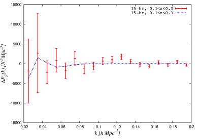
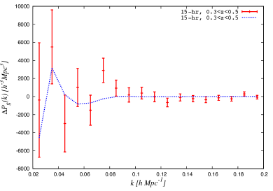
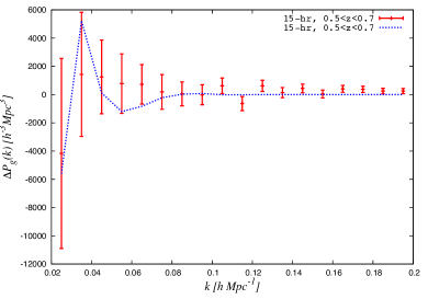
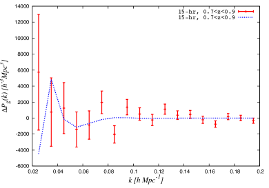
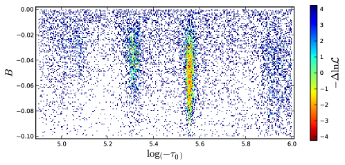
Based on the findings of the previous study Achucarro:2013cva ; Achucarro:2014msa with Planck temperature-temperature power spectrum, we sample the same region of the parameter space using only the galaxy power spectrum from the WiggleZ Dark Energy Survey. As an example, Fig. 1 shows residuals in the convolved galaxy power spectra, eq. 8, of the feature model with parameter values , , , against the base CDM model in four redshift bins, with data points coming from the 15-hr region of the WiggleZ survey. The full set of the power spectra residual from all the seven fields can be found at http://wwwhome.lorentz.leidenuniv.nl/~hu/links/wigglez_res/. The parameter estimation result is shown in Fig. 2(a). In particular we show the profile likelihood of the sample in the plane . The upper limit of has been slightly extended, and the lower one slightly shrunk, in order to limit the interval to the region in which the improvement in the likelihood is significant (but we will later restore the limits of Achucarro:2013cva in the evidence computation). As of the role of nuisance parameters, similarly to the results in reference Achucarro:2013cva , no significant impact on the confidence level for the features’ parameters are reported.
As we can see, in the WiggleZ posterior there exist three diffused modes. In particular, comparing Figs. 2(a) and 2(b) with the naked eye there seems to exist a coincidence between WiggleZ and Planck results around , and , which were three of the most significant modes detected in the previous work Achucarro:2013cva , named respectively modes , and . In order to test such coincidence, we repeated the search combining both data sets. The results are reported in Fig. 2(c). The well-isolated modes previously found in the Planck data are accurately reproduced (compare Figs. 2(b) and 2(c), and also see Fig. 3(a)). In addition we observe an unfolding of mode and a new mode at which survives the addition of the WiggleZ data; both of them will be the subject of future work. We have checked that there exists an enhancement of more than in the value of the likelihood improvement () in modes and , while that of mode shows no enhancement.
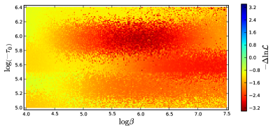
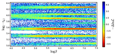
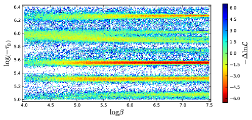
At this point, let us notice two interesting characteristics of the posterior of the feature model which are present using any combination of the Planck and WiggleZ data sets. In the first place, the posterior is multi-modal in all cases. The multi-modality is due to fitting a signal with a size comparable to the noise level of the data. Second, almost every mode is elongated along the direction, due to a degeneracy between and that was already discussed in Achucarro:2014msa in the context of Planck data only, and is not alleviated by including WiggleZ data.
Later, we isolated and resampled using MCMC methods each of the four individual modes found in Achucarro:2013cva (see Fig. 3) with the joint data sets. The corresponding results are shown in the Fig. 3(a). We can see that the individual modes are separated quite well in the direction.
If we force ourselves to focus on one particular mode, such as mode , we can obtain quite stringent constraints on the feature parameters, like those demonstrated in Fig. 7 of reference Achucarro:2014msa . However, finding stringent constraints does not mean that this result has a very strong statistical significance, because the parameter space volume of the feature model is much larger than that of the vanilla model. So, even if there exists a local patch in the parameter space with highly peaked likelihood, the evidence of this signature could still be suppressed greatly by the big volume of the extra parameter space, as discussed in the previous section.
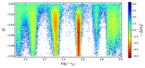
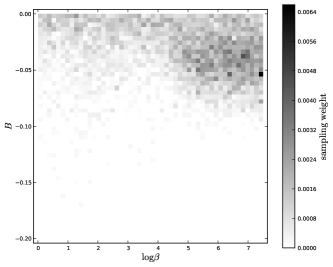
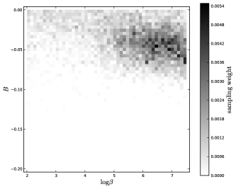
Inspired by the fact that there exists a relatively significant reduction in the likelihood value of the feature model in the best fits compared with that of the featureless model, (e.g. for mode the joint data analysis gives ), we are motivated to compute the Bayesian ratio of the feature model. The statistical results are summarized in Tab. 2, Fig. 3(b) and Fig. 4.
A comparison between the results of the MCMC and multimodal nested samplings, showing the consistency between them, can be seen in Fig. 3. The main difference between both subplots is due to the more thorough sampling of the tails of the distribution (points in parameter space with low likelihood value) achieved by multi-modal nested sampling: these points are crucial to get a reliable evidence estimation, which is the goal of the nested-sampling algorithms, but almost irrelevant to parameter estimation, at which MCMC excel. In Tab. 2, we can see that the resulting best fit likelihood values from multimodal nested sampling are also consistent with those coming from MCMC sampling, though, as expected, the former a little bit lower than the latter, since the sampling around the maxima is more thorough in MCMC’s.
In the first place, the Bayesian ratios listed in Tab. 2 tell us that there exists apparently a slightly positive preference for the feature model: vs. . However, according to the conventional criterion Jeffreys it means that the preference is barely worth mentioning. We must emphasize that in this paper we did not cover all the parameter regime allowed by theory, which sets no lower bound for , but instead the regime in which the features are most likely to be detectable by Planck. Despite the expected corrections, the slightly favourable value of the Bayesian evidence in the observable regime makes us optimistic about the enlargement of the parameter space and the addition of new data sets, namely Planck’s polarization power spectrum and bispectrum. This optimistism is also backed up by how, as discussed in the Sec. III, the increase in the Bayesian ratio when adding the WiggleZ data indicates a positive correlation between the features found in both data sets; nevertheless, when put into the context of the error bars for the evidences cited in table 2, the claim gets milder.
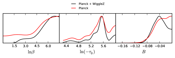
Also, on the positive side, as can be seen in Fig. 4, the addition of the WiggleZ data set clearly pushes the marginalised distribution towards bigger amplitudes of the feature with respect to using Planck data only, which on the one hand is an indication of a positive correlation between the sets, and on the other hand reinforces the overall likelihood of the presence of a feature against the null hypothesis.
| Model | Data set | |||
|---|---|---|---|---|
| Planck | () | |||
| Planck | () | |||
| PlanckWiggleZ | () | |||
| PlanckWiggleZ | () |
V Conclusions and outlook
In this paper we searched for primordial oscillatory signals inspired by a transient reduction in the sound speed of the adiabatic curvature perturbation via CMB (Planck) and LSS (WiggleZ) windows. First of all, by analysing both data sets separately, we found some common oscillatory patterns both in the Planck CMB temperature-temperature power spectrum and the WiggleZ galaxy spectrum. Interestingly, we found a coincidence in the most significant mode previously found by Achúcarro et al. 2013 Achucarro:2013cva by using only Planck data. Second, the joint data analysis showed that the oscillation frequency of the feature gets better constrained, and the amplitude marginally deviates from zero, unlike what was observed by using only Planck data. Besides parameter estimation, we also calculated the Bayesian evidence for the purpose of model selection by using multimodal nested sampling. The results suggest that there exist a slightly positive preference for the feature model, Bayesian factor vs. . However, according to Jeffreys’s criterion it means barely worth mentioning.
Despite the coincidence between both data sets, we notice that the addition of LSS data does not lead to significantly higher predictivity. In theory, the galaxy surveys, compared with the CMB measurements, should be more robust at constraining features existing on scales between tens and hundreds of Mpc, due to the fact that matter perturbations are not damped inside the sound horizon at the epoch of recombination, while they are in the photon temperature anisotropies. Nevertheless, with the present sky coverage of LSS surveys, the sample variance still dominates the uncertainties on the large scales. In order to reach a sensitivity level similar to Planck’s, we need full-sky coverage and deep redshift galaxy surveys, such as Euclid.
The Bayesian evidence analysis shows that although there exists a relatively large improvement in the likelihood value () in several particular parameter regimes, due to the relatively large number of extra parameters () and their broad ranges of variation (look-elsewhere effect), the present Planck temperature-temperature and WiggleZ matter power spectra data still lack significance to claim a detection. However, due to the correlations between temperature and polarization modes of the power spectrum and the correlations with the bispectra given by the model of transient reductions in the speed of sound, the present results have specific predictions for the TE cross-correlation spectrum () Achucarro:2014msa and the temperature bispectrum () Achucarro:2013cva ; Achucarro:2014msa . Particularly, the new fast bispectrum estimator of oscillatory features from Munchmeyer:2014nqa should be able to cover the frequency where the most significant mode that we found is located. If those predictions are right, these signals in polarisation spectra and temperature bispectrum may be observed with the upcoming Planck data release in 2015, though it is by now unclear whether the sensitivity level of the Planck full-mission data will be high enough to claim a detection.
In the light of the additional WiggleZ data, we update the predictions stated in Achucarro:2013cva ; Achucarro:2014msa , based on the high correlation between the bispectrum features studied there and the phenomenological oscillatory shape tested by the Planck collaboration and given in (Ade:2013ydc, , eq. (16)).888For every combination of the feature parameter values in the regions of high likelihood, one can find a combination of the parameters in Ade:2013ydc (including a gaussian envelope as described there) such that the correlation between both shapes at the primordial level is al least . In the parameters used by the Planck collaboration, we expect to find a feature with zero phase, and wavelength in the c.l. interval from mode , or from mode . As happened when using only Planck data Achucarro:2014msa , a degeneracy between and prevents us from setting accurate predictions for the amplitude and envelope of the feature. Nevertheless, for all values of the parameters along the degeneracy, the signal is most significant on the scales beyond the second acoustic peak, and reaches its maximum around the third or fourth peak.
Acknowledgements.
We are indebted to Ana Achúcarro, Enrico Pajer, Pablo Ortiz and Vicente Atal for helpful discussion. BH thanks Alan Heavens for helpful correspondence. This work is supported by the Dutch Foundation for Fundamental Research on Matter (FOM).References
- (1) C. L. Bennett et al. [WMAP Collaboration], Astrophys. J. Suppl. 208, 20 (2013) [arXiv:1212.5225 [astro-ph.CO]].
- (2) P. A. R. Ade et al. [Planck Collaboration], Astron. Astrophys. 571, A22 (2014) [arXiv:1303.5082 [astro-ph.CO]].
- (3) P. A. R. Ade et al. [Planck Collaboration], Astron. Astrophys. 571, A24 (2014) [arXiv:1303.5084 [astro-ph.CO]].
- (4) A. Achucarro, J. -O. Gong, G. A. Palma and S. P. Patil, Phys. Rev. D 87, 121301 (2013) [arXiv:1211.5619 [astro-ph.CO]].
- (5) A. Achucarro, V. Atal, P. Ortiz and J. Torrado, Phys. Rev. D 89, 103006 (2014) [arXiv:1311.2552 [astro-ph.CO]].
- (6) A. Achucarro, V. Atal, B. Hu, P. Ortiz and J. Torrado, Phys. Rev. D 90, 023511 (2014) [arXiv:1404.7522 [astro-ph.CO]].
- (7) A. A. Starobinsky, JETP Lett. 55, 489 (1992) [Pisma Zh. Eksp. Teor. Fiz. 55, 477 (1992)].
- (8) J. A. Adams, B. Cresswell and R. Easther, Phys. Rev. D 64, 123514 (2001) [astro-ph/0102236].
- (9) J. O. Gong, JCAP 0507, 015 (2005) [astro-ph/0504383].
- (10) X. Chen, R. Easther and E. A. Lim, JCAP 0804, 010 (2008) [arXiv:0801.3295 [astro-ph]].
- (11) F. Arroja, A. E. Romano and M. Sasaki, Phys. Rev. D 84, 123503 (2011) [arXiv:1106.5384 [astro-ph.CO]].
- (12) J. Martin and L. Sriramkumar, JCAP 1201, 008 (2012) [arXiv:1109.5838 [astro-ph.CO]].
- (13) P. Adshead, C. Dvorkin, W. Hu and E. A. Lim, Phys. Rev. D 85, 023531 (2012) [arXiv:1110.3050 [astro-ph.CO]].
- (14) F. Arroja and M. Sasaki, JCAP 1208, 012 (2012) [arXiv:1204.6489 [astro-ph.CO]].
- (15) N. Bartolo, D. Cannone and S. Matarrese, JCAP 1310, 038 (2013) [arXiv:1307.3483 [astro-ph.CO]].
- (16) D. Cannone, N. Bartolo and S. Matarrese, Phys. Rev. D 89, 127301 (2014) [arXiv:1402.2258 [astro-ph.CO]].
- (17) L. Covi, J. Hamann, A. Melchiorri, A. Slosar and I. Sorbera, Phys. Rev. D 74, 083509 (2006) [astro-ph/0606452].
- (18) M. Benetti, M. Lattanzi, E. Calabrese and A. Melchiorri, Phys. Rev. D 84, 063509 (2011) [arXiv:1107.4992 [astro-ph.CO]].
- (19) M. Benetti, Phys. Rev. D 88, 087302 (2013) [arXiv:1308.6406 [astro-ph.CO]].
- (20) J. Hamann, L. Covi, A. Melchiorri and A. Slosar, Phys. Rev. D 76, 023503 (2007) [astro-ph/0701380].
- (21) M. Benetti, S. Pandolfi, M. Lattanzi, M. Martinelli and A. Melchiorri, Phys. Rev. D 87, 023519 (2013) [arXiv:1210.3562 [astro-ph.CO]].
- (22) E. D. Stewart, Phys. Rev. D 65, 103508 (2002) [astro-ph/0110322].
- (23) J. Choe, J. O. Gong and E. D. Stewart, JCAP 0407, 012 (2004) [hep-ph/0405155].
- (24) C. Dvorkin and W. Hu, Phys. Rev. D 81, 023518 (2010) [arXiv:0910.2237 [astro-ph.CO]].
- (25) P. Adshead, W. Hu, C. Dvorkin and H. V. Peiris, Phys. Rev. D 84, 043519 (2011) [arXiv:1102.3435 [astro-ph.CO]].
- (26) V. Miranda, W. Hu and P. Adshead, Phys. Rev. D 86, 063529 (2012) [arXiv:1207.2186 [astro-ph.CO]].
- (27) P. Adshead, W. Hu and V. Miranda, Phys. Rev. D 88, no. 2, 023507 (2013) [arXiv:1303.7004 [astro-ph.CO]].
- (28) U. H. Danielsson, Phys. Rev. D 66, 023511 (2002) [hep-th/0203198].
- (29) B. R. Greene, K. Schalm, G. Shiu and J. P. van der Schaar, JCAP 0502, 001 (2005) [hep-th/0411217].
- (30) P. D. Meerburg, J. P. van der Schaar and P. S. Corasaniti, JCAP 0905, 018 (2009) [arXiv:0901.4044 [hep-th]].
- (31) M. G. Jackson and K. Schalm, Phys. Rev. Lett. 108, 111301 (2012) [arXiv:1007.0185 [hep-th]].
- (32) X. Gao, D. Langlois and S. Mizuno, JCAP 1210, 040 (2012) [arXiv:1205.5275 [hep-th]].
- (33) X. Gao, D. Langlois and S. Mizuno, JCAP 1310, 023 (2013) [arXiv:1306.5680 [hep-th]].
- (34) R. Saito and Y. i. Takamizu, JCAP 1306, 031 (2013) [arXiv:1303.3839, arXiv:1303.3839 [astro-ph.CO]].
- (35) T. Noumi and M. Yamaguchi, JCAP 1312, 038 (2013) [arXiv:1307.7110 [hep-th]].
- (36) X. Chen and M. H. Namjoo, Phys. Lett. B 739, 285-292 (2014) [arXiv:1404.1536 [astro-ph.CO]].
- (37) X. Chen and C. Ringeval, JCAP 1208, 014 (2012) [arXiv:1205.6085 [astro-ph.CO]].
- (38) J. Martin and C. Ringeval, Phys. Rev. D 69, 083515 (2004) [astro-ph/0310382].
- (39) R. Flauger, L. McAllister, E. Pajer, A. Westphal and G. Xu, JCAP 1006, 009 (2010) [arXiv:0907.2916 [hep-th]].
- (40) R. Flauger and E. Pajer, JCAP 1101, 017 (2011) [arXiv:1002.0833 [hep-th]].
- (41) M. Aich, D. K. Hazra, L. Sriramkumar and T. Souradeep, Phys. Rev. D 87, 083526 (2013) [arXiv:1106.2798 [astro-ph.CO]].
- (42) P. D. Meerburg, R. Wijers and J. P. van der Schaar, Mon. Not. Roy. Astron. Soc. 421 369-380 (2012) [arXiv:1109.5264 [astro-ph.CO]].
- (43) H. Peiris, R. Easther and R. Flauger, JCAP 1309, 018 (2013) [arXiv:1303.2616 [astro-ph.CO]].
- (44) P. D. Meerburg, D. N. Spergel and B. D. Wandelt, Phys. Rev. D 89, 063536 (2014) [arXiv:1308.3704 [astro-ph.CO]].
- (45) P. D. Meerburg and D. N. Spergel, Phys. Rev. D 89, 063537 (2014) [arXiv:1308.3705 [astro-ph.CO]].
- (46) A. Achucarro, J. O. Gong, S. Hardeman, G. A. Palma and S. P. Patil, JCAP 1101, 030 (2011) [arXiv:1010.3693 [hep-ph]].
- (47) W. Hu, Phys. Rev. D 84, 027303 (2011) [arXiv:1104.4500 [astro-ph.CO]].
- (48) M. Park and L. Sorbo, Phys. Rev. D 85, 083520 (2012) [arXiv:1201.2903 [astro-ph.CO]].
- (49) M. Nakashima, R. Saito, Y. i. Takamizu and J. Yokoyama, Prog. Theor. Phys. 125, 1035 (2011) [arXiv:1009.4394 [astro-ph.CO]].
- (50) R. Bean, X. Chen, G. Hailu, S.-H. H. Tye and J. Xu, JCAP 0803, 026 (2008) [arXiv:0802.0491 [hep-th]].
- (51) R. H. Ribeiro, JCAP 1205, 037 (2012) [arXiv:1202.4453 [astro-ph.CO]].
- (52) P. D. Meerburg, Phys. Rev. D 82, 063517 (2010) [arXiv:1006.2771 [astro-ph.CO]].
- (53) P. D. Meerburg, D. N. Spergel and B. D. Wandelt, arXiv:1406.0548 [astro-ph.CO].
- (54) A. Achucarro, J. O. Gong, S. Hardeman, G. A. Palma and S. P. Patil, Phys. Rev. D 84, 043502 (2011) [arXiv:1005.3848 [hep-th]].
- (55) S. Cespedes, V. Atal and G. A. Palma, JCAP 1205, 008 (2012) [arXiv:1201.4848 [hep-th]].
- (56) A. Achucarro, J. O. Gong, S. Hardeman, G. A. Palma and S. P. Patil, JHEP 1205, 066 (2012) [arXiv:1201.6342 [hep-th]].
- (57) A. Lewis, A. Challinor and A. Lasenby, Astrophys. J. 538, 473 (2000), [astro-ph/9911177].
- (58) A. Lewis and S. Bridle, Phys. Rev. D 66, 103511 (2002) [astro-ph/0205436].
- (59) F. Feroz, M. P. Hobson and M. Bridges, Mon. Not. Roy. Astron. Soc. 398, 1601 (2009) [arXiv:0809.3437 [astro-ph]].
- (60) F. Feroz and M. P. Hobson, Mon. Not. Roy. Astron. Soc. 384, 449 (2008) [arXiv:0704.3704 [astro-ph]].
- (61) Feroz F., Hobson M. P., Cameron E., Pettitt A. N., 2013, arXiv, [arXiv:1306.2144 [astro-ph.IM]].
- (62) P. A. R. Ade et al. [Planck Collaboration], Astron. Astrophys. 571, A16 (2014) [arXiv:1303.5076 [astro-ph.CO]].
- (63) P. A. R. Ade et al. [Planck Collaboration], Astron. Astrophys. 571, A15 (2014) [arXiv:1303.5075 [astro-ph.CO]].
- (64) D. Parkinson, S. Riemer-Sorensen, C. Blake, G. B. Poole, T. M. Davis, S. Brough, M. Colless and C. Contreras et al., Phys. Rev. D 86, 103518 (2012) [arXiv:1210.2130 [astro-ph.CO]].
- (65) M. J. Drinkwater, R. J. Jurek, C. Blake, D. Woods, K. A. Pimbblet, K. Glazebrook, R. Sharp and M. B. Pracy et al., Mon. Not. Roy. Astron. Soc. 401, 1429 (2010) [arXiv:0911.4246 [astro-ph.CO]].
- (66) C. Blake, S. Brough, M. Colless, W. Couch, S. Croom, T. Davis, M. J. Drinkwater and K. Forster et al., Mon. Not. Roy. Astron. Soc. 406, 803 (2010) [arXiv:1003.5721 [astro-ph.CO]].
- (67) S. Riemer-Sørensen, D. Parkinson and T. M. Davis, Phys. Rev. D 89 103505 (2014) [arXiv:1306.4153 [astro-ph.CO]].
- (68) Skilling J., 2004, AIP Conference Proceedings of the 24th International Workshop on Bayesian Inference and Maximum Entropy Methods in Science and Engineering, Vol. 735, pp. 395-405
- (69) Sivia D., Skilling J., 2006, Data Analysis; a Bayesian tutorial, 2nd ed., Oxford University Press, Oxford
- (70) P. Mukherjee, D. Parkinson and A. R. Liddle, Astrophys. J. 638 (2006) L51 [astro-ph/0508461].
- (71) A. R. Liddle, Mon. Not. Roy. Astron. Soc. 377, L74 (2007) [astro-ph/0701113].
- (72) R. Shaw, M. Bridges and M. P. Hobson, Mon. Not. Roy. Astron. Soc. 378, 1365 (2007) [astro-ph/0701867 [ASTRO-PH]].
- (73) S. H. Jeffreys, The Theory of Probability (Oxford University Press, New York, NY, USA, 1961).
- (74) M. Münchmeyer, F. Bouchet, M. Jackson and B. Wandelt, Astron. Astrophys. 570 A94 (2014) [arXiv:1405.2550 [astro-ph.CO]].