Higher Criticism for Large-Scale Inference, Especially for Rare and Weak Effects

Abstract

In modern high-throughput data analysis, researchers perform a large number of statistical tests, expecting to find perhaps a small fraction of significant effects against a predominantly null background. Higher Criticism (HC) was introduced to determine whether there are any nonzero effects; more recently, it was applied to feature selection, where it provides a method for selecting useful predictive features from a large body of potentially useful features, among which only a rare few will prove truly useful.

In this article, we review the basics of HC in both the testing and feature selection settings. HC is a flexible idea, which adapts easily to new situations; we point out simple adaptions to clique detection and bivariate outlier detection. HC, although still early in its development, is seeing increasing interest from practitioners; we illustrate this with worked examples. HC is computationally effective, which gives it a nice leverage in the increasingly more relevant “Big Data” settings we see today.

We also review the underlying theoretical “ideology” behind HC. The Rare/Weak (RW) model is a theoretical framework simultaneously controlling the size and prevalence of useful/significant items among the useless/null bulk. The RW model shows that HC has important advantages over better known procedures such as False Discovery Rate (FDR) control and Family-wise Error control (FwER), in particular, certain optimality properties. We discuss the rare/weak phase diagram, a way to visualize clearly the class of RW settings where the true signals are so rare or so weak that detection and feature selection are simply impossible, and a way to understand the known optimality properties of HC.

FLA

Special Invited Paper

and

1 Introduction

A data deluge is now flooding scientific and technical work datadeluge . In field after field, high-throughput devices gather many measurements per individual; depending on the field, these could be gene expression levels, or spectrum levels, or peak detectors or wavelet transform coefficients; there could be thousands or even millions of different feature measurements per single subject.

High-throughput measurement technology automatically measures systematically generated features and contrasts; these features are not custom-designed for any one project. Only a small proportion of the measured features are expected to be relevant for the research in question, but researchers do not know in advance which those will be; they instead measure every contrast fitting within their systematic scheme, intending later to identify a small fraction of relevant ones post-facto.

This flood of high-throughput measurements is driving a new branch of statistical practice: what Efron EfronLSI calls Large-Scale Inference (LSI). For this paper, two specific LSI problems are of interest:

• Massive multiple testing for sparse intergroup differences. Here we have two groups, a treatment and a control, and for each measured variable we test whether the two groups are different on that measurement, obtaining, say, a $P$-value per feature. Of course, many individual features are unrelated to the specific intervention being studied, and those would be expected to show no significant differences—but we do not know which these are. We expect that even when there are true inter-group differences, only a small fraction of measured features will be affected—but, again, we do not know which features they are. We therefore use the whole collection of $P$-values to correctly decide if there is any difference between the two groups.

• Sparse feature selection. A large number of features are available for training a linear classifier, but we expect that most of those features are in fact useless for separating the underlying classes. We must decide which features to use in designing a class prediction rule.

Higher Criticism (HC) and its elaborations can be useful in both of these LSI settings; under a particular asymptotic model discussed below—the Asymptotic Rare/Weak (ARW) model—HC offers theoretical optimality in selecting features. In this paper we will review the basic notions of HC, some variations and settings where it applies. HC is a flexible idea and can be adapted to a range of new problem areas; we briefly discuss three simple examples.

1.1 HC Basics

John Tukey Tukey76 , Tukey89 , Tukey94 coined the term “Higher Criticism” and motivated it by the following story. A young scientist administers a total of $250$ independent tests, out of which $11$ are significant at the level of $5\%$. The youngster is excited about the findings and plans to trumpet them until a senior researcher tells him that, even in the purely null case, one would expect to have $12.5$ significances. In that sense, finding only $11$ significances is actually disappointing. Tukey proposes a kind of second-level significance testing, based on the statistic

$$\mathrm{HC}_{N,0.05} = \sqrt{N}(\mbox{Fraction significant at $5\%$}-0.05)$$

$${}/\sqrt{0.05\times 0.95},$$

where $N=250$ is the total number of tests. Obviously this score has an interpretation similar to $Z$- and $t$- statistics, so Tukey suggests that a value of $2$ or larger indicates significance of the overall body of tests. In Tukey’s example,

$$\mathrm{HC}_{N,0.05}=-0.43.$$

If the young researcher really “had something” this score should be strongly positive, for example, $2$ or more, but here the score is negative, implying that the overall body of the evidence is consistent with the null hypothesis of no difference. Donoho and Jin DJ04 saw that in the modern context of large $N$ and rare/weak signals, it was advantageous to generalize beyond the single significance level $\alpha=0.05$. They maximized over all levels $\alpha$ between $0$ and some preselected upper bound $\alpha_{0}\in(0,1)$. So generalize Tukey’s proposal and set

$$\mathrm{HC}_{N,\alpha} = \sqrt{N}(\mbox{Fraction significant at $\alpha$}-\alpha)$$

$${}/\sqrt{\alpha\times(1-\alpha)}.$$

If the overall body of tests is significant, then we expect $\mathrm{HC}_{N,\alpha}$ to be large for some $\alpha$. Otherwise, we expect $\mathrm{HC}_{N,\alpha}$ to be small over all $\alpha$ in a wide range. In other words, the significance of the overall body of test is captured in the following Higher Criticism statistic:

$$\mathrm{HC}_{N}^{*}=\max_{\{0\leq\alpha\leq\alpha_{0}\}}\mathrm{HC}_{N,\alpha},$$ (1)

where $\alpha_{0}\in(0,1)$ is a tuning parameter we often set at $\alpha_{0}=1/2$.

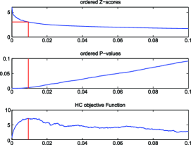
Figure 1: Illustration of HC. The component score maximizing the HC objective is located at the red line. Bottom panel: the HC objective function $\mathrm{HC}_{N,i}$ versus $i/N$. Middle panel: the underlying $P$-vales $\pi_{(i)}$ versus $i/N$. Top panel: the corresponding ordered $Z$-scores $z_{(i)}$ versus $i/N$.

Higher Criticism (HC) can be computed efficiently as follows. Consider a total of $N$ uncorrelated tests:

• For $i=1,2,\ldots,N$, get the corresponding individual $P$-values $\pi_{i}$, producing in all a body of $P$-values $\pi_{1},\pi_{2},\ldots,\pi_{N}$.

• Sort the $P$-values in the ascending order:

  $$\pi_{(1)}<\pi_{(2)}<\cdots<\pi_{(N)}.$$

• The Higher Criticism statistic in (1) can be equivalently written as follows:

  $$\mathrm{HC}_{N}^{*} = \max_{\{1\leq i\leq\alpha_{0}N\}}\mathrm{HC}_{N,i},$$

  $$\mathrm{HC}_{N,i} \equiv \sqrt{N}\frac{(i/N)-\pi_{(i)}}{\sqrt{\pi_{(i)}(1-\pi_{(i)})}}.$$

In words, we are looking at a test for equality of a binomial proportion $\pi_{(i)}$ to an expected value $i/N$, maximizing this statistic across a range of $i$. We think that the evidence against being purely null is located somewhere in this range, but we cannot say in advance where that might be. The computational cost of $\mathrm{HC}$ is $O(N\log(N))$ and is moderate.

Figure 1 illustrates the definition of Higher Criticism. Consider an example where the (one-sided) $P$-values $\pi_{i}$ are produced by $Z$-values $z_{i}$ through $\pi_{i}=1-\Phi(z_{i})$, $1\leq i\leq N$, where $\Phi$ denotes the CDF of $N(0,1)$. The first panel shows the sorted $Z$-values in the descending order, the second panel shows the sorted $P$-values, and the last panel shows $\mathrm{HC}_{N,i}$. In this example, $\mathrm{HC}_{N}^{*}=7.1$, reached by $\mathrm{HC}_{N,i}$ at $i=0.0085\times N$.

Asymptotic theory shows that the component scores $\mathrm{HC}_{N,i}$ can be poorly behaved for $i$ very small (e.g., $1$ or $2$). We often recommend the following modified version:

$$\mathrm{HC}_{N}^{+}=\max_{\{1\leq i\leq\alpha_{0}N\dvtx\pi_{(i)}>1/N\}}\mathrm{HC}_{N,i}.$$

As the last remark illustrates, small variations on the above prescription will sometimes be useful, for example, the modification of the underlying $Z$-like scores, in (2.7)–(2.7) below. Moreover, several other statistics such as Berk–Jones and Average Likelihood Ratio offer cognates or substitutes; see Section 2.7 below. The real point of HC is less the specific definition (• ‣ 1.1) and more a viewpoint about the nature of evidence against the null hypothesis, namely, that although the evidence may be cumulatively substantial, it is diffuse, individually very weak and affecting a relatively small fraction of the individual $P$-values or $Z$-scores in our study.

So HC can be viewed as a family of methods for which the above definitions give a convenient entry point. To make utterly clear, when needed we label definition (• ‣ 1.1) the Orthodox Higher Criticism (OHC).

1.2 The Rare/Weak Effects Viewpoint and Phase Diagram

Effect sparsity was proposed as a useful hypothesis already in the 1980s by Box and Meyer Box ; it proposes that relatively few of the observational units or factorial levels can be expected to show any difference from a global null hypothesis of no effect, and that a priori we have no opinion about which units or levels those might be.

The Effect weakness hypothesis assumes that individual effects are not individually strong enough to be detectable, once traditional multiple comparisons ideas are taken into account.

The Rare/Weak viewpoint combines both hypotheses in analysis of large-scale experiments; it is intended to be a flexible concept and to vary from one setting to another.

The next section operationalizes these ideas in a specific model, where $N$ independent $Z$-scores follow a mixture with a fraction $(1-\varepsilon)$ which are truly null effects and so distributed $N(0,1)$, while the remaining $\varepsilon$ fraction have a common effect size $\tau$ and are distributed $N(\tau,1)$. In this situation, the Rare/Weak viewpoint studies the regime where $\varepsilon$ is small, the locations of the nonzero effects are scattered irregularly through the scores and the effect size $\tau$ is, at moderate $N$, only $2$ or $3$ standard deviations.

For large $N$ one can develop a precise theory; see Section 6 below. There we develop the Asymptotic Rare/Weak (ARW) model, a framework that assigns parameters to the rare and weak attributes of a nonnull situation; a key phenomenon is that in the two-dimensional parameter space there are three separate regions (or phases) where an inference goal is relatively easy, nontrivial but possible, and impossible to achieve, correspondingly. The ARW phase diagram offers revealing comparisons between HC and other seemingly similar methods, such as FDR control.

2 HC for Detecting Sparse and Weak Effects

In DJ04 Higher Criticism was originally proposed for detecting sparse Gaussian mixtures. Suppose we have $N$ test statistics $X_{i}$, $1\leq i\leq N$ (reflecting many individual genes, voxels, etc.). Suppose that these tests are standardized so that each individual test, under its corresponding null hypothesis, would have mean 0 and standard deviation 1. We are interested in testing whether all test statistics are distributed $N(0,1)$ versus the alternative that a small fraction is distributed as normal with an elevated mean $\tau$. In effect, we want an overall test of a complete null hypothesis:

$$H_{0}^{(N)}\dvtx\quad X_{i}\stackrel{{\scriptstyle\mathrm{i.i.d.}}}{{\sim}}N(0,1),\quad 1\leq i\leq N,$$ (3)

against an alternative in its complement,

$$\quad H_{1}^{(N)}\dvtx\quad X_{i}\stackrel{{\scriptstyle\mathrm{i.i.d.}}}{{\sim}}(1-\varepsilon)N(0,1)+\varepsilon N(\tau,1),$$

(4)

$$\eqntext{1\leq i\leq N.}$$ (5)

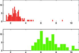
Figure 2: Simulated Higher Criticism values. Top panel: simulation under null hypothesis $H_{0}^{(N)}$. Bottom panel: simulation under alternative hypothesis $H_{1}^{(N)}$.

To use HC for such a case, we calculate the (one-sided) $P$-values by

$$\pi_{i}=1-\Phi(X_{i}),\quad 1\leq i\leq N.$$

We then apply the basic definition of HC to the collection of $P$-values.

In Figure 2, we show the simulated HC values of $H_{0}^{(N)}$ and $H_{1}^{(N)}$ based on $100$ independent repetitions, where the parameters are set as $(N,\varepsilon,\tau)=(10^{6},10^{-3},2)$. It is seen that the simulated HC values under $H_{1}^{(N)}$ are well separated from those under $H_{0}^{(N)}$.

2.1 Critical Value for Using HC as a Level-$\alpha$ Test

Fix $0<\alpha<1$. To use HC as a level-$\alpha$ test, we must find a critical value $h(N,\alpha)$ so that

$$P_{H_{0}^{(N)}}\bigl{\{}\mathrm{HC}_{N}^{*}>h(N,\alpha)\bigr{\}}\leq\alpha.$$

$\mathrm{HC}^{*}_{N}$ can be connected with the maximum of a standardized empirical process; see Donoho and Jin DJ04 . Using this connection, it follows from Wellner86 , page 600, that as $N\rightarrow\infty$, $b_{N}\mathrm{HC}_{N}^{*}-c_{N}$ and $b_{N}\mathrm{HC}_{N}^{+}-c_{N}$ converge weakly to the same limit—the standard Gumbel distribution, where $b_{N}=\sqrt{2\log\log(N)}$ and $c_{N}=2\log\log(N)+(1/2)[\log\log\log(N)-\log(4\pi)]$. As a result, for any fixed $\alpha\in(0,1)$ and $N\rightarrow\infty$,

$$h(N,\alpha) \approx h_{G}(N,\alpha)$$

$$= \sqrt{2\log\log(N)}\bigl{(}1+o(1)\bigr{)},$$

where $h_{G}(N,\alpha)=b_{N}^{-1}[c_{N}-\log\log(\frac{1}{1-\alpha})]$ (“G” stands for Gumbel). When $N$ is moderately large and $\alpha$ is moderately small, the approximations may not be accurate enough, and it is hard to derive an accurate closed-form approximation (even in much simpler cases; see dasgupta for nonasymptotic bound on extreme values of normal samples). In such cases, it is preferable to determine $h(N,\alpha)$ by simulations.

Table 1: Simulated values $h(N,\alpha)$ based on $10^{5}$ repetitions. Numbers in brackets are $h_{G}(N,\alpha)$

		$\bolds{N}$
Level	Statistic	$\bolds{10^{3}}$	$\bolds{5\times 10^{3}}$	$\bolds{2.5\times 10^{4}}$	$\bolds{1.25\times 10^{5}}$
$\alpha=0.05$	$\mathrm{HC}_{N}^{+}$	03.17 (3.00)	03.22 (3.08)	03.26 (3.14)	03.30 (3.19)
	$\mathrm{HC}_{N}^{*}$	04.77 (3.00)	04.73 (3.08)	04.74 (3.14)	04.75 (3.19)
$\alpha=0.01$	$\mathrm{HC}_{N}^{+}$	03.95 (3.83)	03.97 (3.87)	03.96 (3.90)	03.99 (3.93)
	$\mathrm{HC}_{N}^{*}$	10.08 (3.83)	09.88 (3.87)	10.20 (3.90)	09.92 (3.93)
$\alpha=0.005$	$\mathrm{HC}_{N}^{+}$	04.29 (4.18)	04.28 (4.20)	04.26 (4.22)	04.28 (4.24)
	$\mathrm{HC}_{N}^{*}$	13.78 (4.18)	14.39 (4.20)	14.34 (4.22)	13.95 (4.24)
$\alpha=0.001$	$\mathrm{HC}_{N}^{+}$	05.03 (5.00)	05.02 (4.98)	04.98 (4.97)	0 4.98 (4.97)
	$\mathrm{HC}_{N}^{*}$	30.27 (5.00)	30.36 (5.02)	31.95 (4.97)	31.49 (4.97)

Table 2: MPM: malignant pleural mesothelioma. ADCA: adenocarcinoma. ALL: acute lymphoblastic leukemia. AML: acute myelogenous leukemia

Data name	# training samples	# test samples	# genes
Leukemia	27 (ALL), 11 (AML)	20 (ALL), 14 (AML)	0.3571
Lung cancer	16 (MPM), 16 (ADCA)	15 (MPM), 134 (ADCA)	12,533

Table 1 displays $h_{G}(N,\alpha)$ and $h(N,\alpha)$ [where $\alpha_{0}=1/2$ as in (1)] computed from $10^{5}$ independent simulations. One sees that: (a) $h_{G}(N,\alpha)$ approximate the percentiles of $\mathrm{HC}_{N}^{*}$ poorly, but approximate those of $\mathrm{HC}_{N}^{+}$ reasonably well, especially when $N$ get larger and $\alpha$ get smaller; (b) the tail of $\mathrm{HC}_{N}^{*}$ is fat but that of $\mathrm{HC}_{N}^{+}$ is relatively thin; (c) the percentiles of $\mathrm{HC}_{N}^{+}$ and $\mathrm{HC}_{N}^{*}$ increase with $N$ only very slowly, therefore, the values of $h(N,\alpha)$ for a few selected $N$ represent those of a wide range of $N$. Very recently, Li and Siegmund LiSiegmund proposed a new approximation to $h(N,\alpha)$ which is more accurate when $N$ is moderately large.

2.2 Two Gene Microarray Data Sets

In Sections 2.3.1 and 3.1, we use two standard gene microarray data sets to help illustrate the use of HC: the lung cancer data analyzed by Gordon et al. lungcancer , and the leukemia data analyzed by Golub et al. leukemia (for the latter, we use the cleaned version published by Dettling Dettling , which contains measurements for $3571$ genes). Both data sets are available at http://www.stat.cmu.edu/
~jiashun/Research/software/. See Table 2, where the partition of samples into the training set and the test set is the same as in lungcancer and leukemia , respectively.

2.3 Detecting Rare and Weak Effects in Genomics and Genetics

When the genomics revolution began 10–15 years ago, many scientists were hopeful that the common disease-common variant hypothesis CDCVH would apply. Under this hypothesis, there would be, for each common disease, a specific gene that is clearly responsible. Such hopes were dashed over the coming years, and, today, much research starts from the hypothesis that numerous genes are differentially expressed in affected patients Goldstein , but with individually small effect sizes Dai , CDRVH . HC, with its emphasis on detecting rare and weak effects, seems well suited to this new environment.

2.3.1 Two worked examples

Let’s apply HC to the two gene microarray data sets. For each in turn, let $x_{ij}$ denote the expression level for the $i$th sample and the $j$th gene, $1\leq i\leq n$, $1\leq j\leq p$. Let $C$ and $D$ be the set of indices of samples from the training set and the test set, respectively. For notational consistency with later sections, we only use the data in the training set, but using the whole data gives similar results.

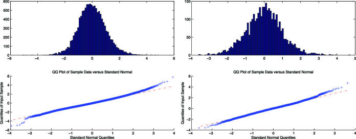
Figure 3: Left column: histogram (top) and $qq$-plot (bottom) of $Z=(Z_{1},Z_{2},\ldots,Z_{p})^{\prime}$ for the lung cancer data set. Right: corresponding plots for the leukemia data set.

Write $C=C_{1}\cup C_{2}$, where $C_{1}$ and $C_{2}$ are the sets of indices of the training samples from classes $1$ and $2$, respectively. Fix $1\leq j\leq p$. Let $\bar{x}_{jk}=\frac{1}{|C_{k}|}\sum_{j\in C_{k}}x_{ij}$ denote the average expression value of gene $j$ for all samples in class $k$, $k=1,2$, and $s_{j}^{2}=\frac{1}{(|C|-2)}[\sum_{i\in C_{1}}(x_{ij}-\bar{x}_{j1})^{2}+\sum_{i\in C_{2}}(x_{ij}-\bar{x}_{j2})^{2}]$ the pooled variance. Define the $t$-like statistic

$$z_{j}^{*}=\frac{1}{\sqrt{1/|C_{1}|+1/|C_{2}|}}\frac{\bar{x}_{j1}-\bar{x}_{j2}}{s_{j}},\quad 1\leq j\leq p.$$

In the null case, if the data $\{x_{ij}\}_{1\leq i\leq n,1\leq j\leq p}$ are independent and identically distributed across different genes, and, for each gene $j$, $\{x_{ij}\}_{i=1}^{n}$ are normal samples with the same variance in each class, then $z_{j}^{*}$ has the Student’s $t$-distribution with $df=|C|-2$ when gene $j$ is not differentially expressed. Using this, we may calculate individual $P$-values for each gene and apply HC. However, as pointed out in Efron EfronNull , a problem one frequently encounters in analyzing gene microarray data is the so-called discrepancy between the empirical null and theoretical null, meaning that there is a gap between the aforementioned $t$-distribution and the empirical null distribution associated with $\{z_{j}^{*}\}_{j=1}^{p}$. This gap might be caused by unsuspected between-gene variance components or other factors. We follow Efron’s suggestion and standardize $z_{j}^{*}$:

$$Z_{j}=\frac{z_{j}^{*}-\bar{z}^{*}}{\mathrm{sd}(z^{*})},\quad 1\leq j\leq p,$$ (7)

where $\bar{z}^{*}$ and $\mathrm{sd}(z^{*})$ represent the empirical mean and standard deviation associated with $\{z_{j}^{*}\}_{j=1}^{p}$, respectively. We call $Z_{1},Z_{2},\ldots,Z_{p}$ the standardized $Z$-scores, and believe that in the purely null case they are approximately normally distributed. In Figure 3, we show the histogram (top) and the $qq$-plot (bottom) associated with the standardized $Z$-scores. The figure suggests that, for both data sets, the standardization in (7) is effective.

We apply HC to $\{Z_{j}\}_{j=1}^{p}$ for both the leukemia and the lung cancer data, where the individual (two-sided) $P$-values are obtained assuming $Z_{j}\sim N(0,1)$ if the $j$th gene is not differentially expressed. The resulting HC scores are $6.1057$ and $13.3025$ in two cases. The $P$-values associated with the scores (computed by numerical simulations) are $\approx 5\times 10^{-5}$ and $<10^{-5}$, respectively. They suggest the definite presence of signals, sparsely scattered in the $Z$-vector. And, indeed, the qqplots exhibit a visible “curving away” from the identity lines.

An alternative approach to computing these two $P$-values uses random shuffles. Denote the data matrix by $X=(x_{ij})_{1\leq i\leq n,1\leq j\leq p}$. First, we randomly shuffle the rows of $X$, independently between different columns. For the permuted data, we follow the steps above and calculate the standardized $Z$-vector. Due to our shuffling, the signals wash out and the $Z$-vector can be viewed as containing no effect signals. Next, apply HC to the $Z$-vector, obtaining an HC statistic specific to that shuffle. Repeat the whole process for $1000$ independent shuffles. As a result, we have $1001$ HC scores: one, based on the original data matrix; all others, based on shuffles. The shuffles are used to calculate the $P$-value of the original HC score. For the (training) leukemia data and the (training) lung cancer data, the resultant $P$-values are approximately $0.01$ and $<0.001$, respectively. Both data sets have standardized $Z$-vectors exhibiting very subtle departures from the null hypothesis, but still permit reliable rejection of the null hypothesis.

2.3.2 Applications to genome-wide association study

By now the literature of Genome-wide association studies (GWAS) has several publications applying HC or its relatives. Parkhomenko et al. GWAS1 used HC to detect modest genetic effects in a genome-wide study of rheumatoid arthritis. It was further suggested in Martin et al. Martin that the implementation of HC in GWAS may provide evidence for the presence of additional remaining SNPs modestly associated with the trait.

Sabatti et al. Sabatti used HC in a GWAS for metabolic traits. HC enabled the authors to quantify the strength of the overall genetic signal for each of the nine traits (Triglycerides, HDL$,\ldots$) they were interested in, where, to deal with the possible dependence caused by Linkage Disequilibrium (LD) between SNPs, they computed individual $P$-values by permutations. See also De la Cruz et al. delaCruz where the authors considered the problem of testing whether there are associated markers in a given region or a given set of markers, with applications to analysis of a SNP data set on Crohn’s disease.

Wu et al. Wu adapted HC for detecting rare and weak genetic signals using the information of LD. He and Wu GWAS2 used HC and innovated HC for signal detection for large-scale exonic single-nucleotide polymorphism data, and suggested modifications of HC in such settings.

Motivated by GWAS, Mukherjee et al. Lin considered the signal detection problem using logistic regression coefficients rather than 2-sample $Z$-scores, and discovered an interesting relationship between the sample size and the detectability when both response variable and design variables are discrete. See Section 2.10 for more discussion on signal detection problems associated with regression models. To address applications in GWAS, Roeder and Wasserman RW made an interesting connection between HC and weighted hypothesis testing.

2.3.3 Applications to DNA copy number variation

Computational biology continues to innovate and GWAS is no longer the only game in town. DNA Copy Number Variation (CNV) data grew rapidly in importance after the GWAS era began, and today provide an important window on genetic structural variation. Jeng et al. Jeng1 , Jeng2 applied HC-style thinking to CNV data and proposed a new method called Proportion Adaptive Segment Selection (PASS). PASS can be viewed as a two-way screening procedure for genomic data, which targets both the signal sparsity across different features (SNPs) and the sparsity across different subjects—so-called rare variation in genomics.

2.4 Applications to Cosmology and Astronomy

HC has been applied in several modern experiments in Astronomy and Cosmology, where typically the experiment produces data which can be interpreted as images (of a kind) and where there is a well-defined null hypothesis, whose overthrow would be considered a shattering event.

Studies of the Cosmic Microwave Background (CMB) offer several examples. CMB is a relic of radiation emitted when the Universe was about 370,000 years old. In the simplest “inflation” models, CMB temperature fluctuations should behave as a realization of a zero-mean Gaussian random variable in each pixel. The resulting Gaussian field (on the sphere) is completely determined by its power spectrum. In recent decades, a large number of studies have been devoted to the subject of detecting non-Gaussian signatures (hot spots, cold spots, excess kurtosis$,\ldots$) in the CMB.

Jin et al. Starck , and Cayon et al. Cayon1 (see also Cruz , Cayon2 ), applied HC to standardized wavelet coefficients of CMB data from the Wilkinson Microwave Anisotropy Probe (WMAP). HC would be sensitive to a small collection of such coefficients departing from the standard null, without requiring that individual coefficients depart in a pronounced way. Compared to the kurtosis-based non-Gaussianity detector (widely used in cosmology when the departure from Gaussianity is in the not-very-extreme tails), HC showed superior power and sensitivity, and pointed, in particular, to the cold spot centered at galactic coordinate (longitude, latitude) = $(207.8^{\circ},-56.3^{\circ})$. In Vielva , Vielva reviews the cold spot detection problem and shows that HC rejects Gaussianity, confirming earlier detections by other methods.

Gravitational weak lensing calculations measure the distortion of background galaxies supposedly caused by intervening large-scale structure. Pires et al. Pires applied many non-Gaussianity detectors to weak lensing data, including the empirical Skewness, the empirical Kurtosis and HC, and showed that HC is competitive, while of course being more specifically focused on excess of observations in the tails of the distribution.

Most recently, Bennett et al. Bennett applied the HC ideas to the problem of Gravitational Wave detection. They use HC as a second-pass method operating on $F$-statistic and $C$-statistics (see Bennett for details) for a monochromatic periodic source in a binary system; such statistics contain a large number of relatively weak signals spread irregularly across many frequency bands. They use a modified form of HC, which is both sensitive and robust, and offer a noticeable increase in the detection power (e.g., a $30\%$ increase in detectability for a phase-wandering source over multiple time intervals).

2.5 Applications to Disease Surveillance and Local Anomaly Detection

In disease surveillance, we have aggregated count data $c_{i}$ representing cases of a certain disease (e.g., influenza) by the $i$th spatial region (e.g., zip code), $1\leq i\leq N$. When disease breaks out, the counts will have elevated values in one or a few small geographical regions. Neill and Lingwall Neill0 , Neill use HC for disease surveillance and spatio-temporal cluster detection: they suppose we have historical counts for each spatial location measured over time $t=1,2,\ldots,T$. The $P$-value of $c_{i}$ is calculated by $(d_{i}+1)/(T+1)$, where $d_{i}$ is the number of historical counts larger than $c_{i}$ at the $i$th location.

Disease outbreak detection is a special case of local anomaly detection as studied in Saligrama and Zhao anomaly . Suppose we have a graph $G=(V,E)$ with usual graph metric, where a random variable is associated with each node. A simple scenario of local anomaly they consider assumes that, for all nodes outside the anomaly, the associated random variables have the same density $f_{0}$, and, for nodes inside the anomaly, the associated density is different from $f_{0}$. Saligrama and Zhao anomaly investigate several models and statistics for local anomaly detection; HC is found to be competitive in this setting.

2.6 Estimating the Proportion of Non-Null Effects

As presented so far, HC offers a test statistic. In the setting of Section 2, we sample $X_{i}$ from the two-component mixture

$$\quad X_{i}\stackrel{{\scriptstyle\mathrm{i.i.d.}}}{{\sim}}(1-\varepsilon)N(0,1)+\varepsilon N(\tau,1),$$

(8)

$$\eqntext{1\leq i\leq N.}$$ (9)

The detection problem which HC addresses involves testing $H_{0}^{(N)}\dvtx\varepsilon=0$ versus $H_{1}^{(N)}\dvtx\varepsilon>0$. Alternatively, one could estimate the mixing proportion $\varepsilon$. Motivated by a study of Kuiper Belt Objects (KBO) (e.g., Rice ), Cai et al. CJL (see also Rice ) developed HC into an estimator for $\varepsilon$, focusing on the regime where $\varepsilon>0$ is very small.

In the growing literature of large-scale multiple testing, the problem of estimating the proportion of nonnull effects has attracted considerable attention in the past decade, though sometimes with different goals. For example, rather than knowing the true proportion of nonzero effects, one might only want to estimate the largest proportion within which the false discovery rate can be controlled. The literature along this line connects to the work of Benjamini and Hochberg BH95 on controlling False Discovery Rate (FDR), and Efron EfronNull on controlling the local FDR in gene microarray studies. See CaiJin2010 , JinCai2007 , Jin2008 and references therein.

2.7 Statistics with HC-Like Constructions

HC can be viewed as a measure of the goodness of fit between two distributions, namely, between the distribution $F_{N}$ of the empirical $P$-values and the model uniform distribution $F_{0}$. In this viewpoint, HC is effectively computing the distance measure

$$\mu_{1}(F_{N},F_{0})$$

(10)

$$\quad=\sqrt{N}\cdot\max_{i=1}^{N}\frac{|F_{N}(i/N)-F_{0}(i/N)|}{\sqrt{F_{0}(i/N)(1-F_{0}(i/N))}}$$

(or, more properly, a restricted form, where $i=1$ and $i>\alpha_{0}N$ are omitted in the maximum) or the reverse

$$\mu_{2}(F_{N},F_{0})$$

(11)

$$\quad=\sqrt{N}\cdot\max_{i=1}^{N}\frac{|i/N-F_{0}(\pi_{(i)})|}{\sqrt{F_{0}(\pi_{(i)})(1-F_{0}(\pi_{(i)}))}}.$$

We call these the theoretically standardized and empirically standardized goodness of fit, respectively.

To understand HC, then, one might consider how it differs from other measures of the discrepancy between two distributions. HC includes the element of standardization, which for many readers will suggest comparison to the Anderson–Darling statistic AndersonDarling :

$$A(F_{N},F_{0})=N\cdot\int\frac{|F_{N}(x)-F_{0}(x)|^{2}}{F_{0}(x)(1-F_{0}(x))}\,dx.$$

HC, however, involves maximization rather than integration, which makes it a kind of weighted Kolmogorov–Smirnov statistic. Jager and Wellner Wellner2004 investigated the limiting distribution of a class of weighted Kolmogorov statistics, including HC as a special case.

Another perspective is to view the $P$-values underlying HC as obtained from the normal approximation to a one-sample test for a known binomial proportion, and to consider instead the exact test based on likelihood ratios, or asymptotic tests based instead on KL divergence between the binomial with parameter $\pi_{i}$ and the binomial with parameter $i/N$. This perspective reveals a similarity of HC to the Berk–Jones (BJ) statistic BerkJones . The similarity was carefully studied in DJ04 , Section 1.6; see details therein. Using the divergence $D(p_{0},p_{1})=p_{0}\log(p_{0}/p_{1})+(1-p_{0})\log((1-p_{0})/(1-p_{1}))$, the Berk–Jones statistic can be written as

$$\mathrm{BJ}=\max_{i=1}^{N}N\cdot D(\pi_{i},i/N).$$

Wellner and Koltchinskii WellnerKoltchinskii derive the limiting distribution of the Berk–Jones statistic, finding that it shares many theoretical properties in common with HC.

In Wellner2007 , Jager and Wellner introduced a new family of goodness-of-fit tests based on the $\phi$-divergence, including HC as a special case, and showed all such tests achieve the optimal detection boundary in DJ04 (see the discussion below in Section 6).

Reintroducing the element of integration found in the Anderson–Darling statistic, Walther Walther proposed an Average Likelihood Ratio (ALR) approach. If $\mathrm{LR}_{i,N}$ denotes the usual likelihood ratio for a one-sided test of the binomial proportion, ALR takes the form

$$\mathrm{ALR} = \sum_{i=1}^{\alpha_{0}N}w_{i,N}\mathrm{LR}_{i,N};$$

$$\mathrm{LR}_{i,N} \equiv \exp\bigl{(}N\max\bigl{\{}D(\pi_{i},i/N),0\bigr{\}}\bigr{)},$$

with weights $w_{i,N}=(2i\log(N/3))^{-1}$. Walther shows that ALR compares favorably with HC and BJ for finite sample performance, while having similar asymptotic properties under the ARW model discussed below. See DJ04 , Tukey76 for more discussions on the relative merits of HC, BJ and ALR.

Additionally, as a measure of goodness of fit, HC is closely related to other goodness-of-fit tests, motivated, however, by the goal of optimal detection of presence of mixture components representing rare/weak signals. We remark that the pontogram of Kendall and Kendall Kendall is an instance of HC, applied to a special set of $P$-values.

Gontscharuk et al. Gontscharuk introduced the notion of local levels for goodness-of-fit tests and studied the asymptotic behavior when applying the framework to one version of HC; for HC, the local level associated with $\mathrm{HC}_{N,i}$ and a critical value $\chi$ roughly translates to $P[\mathrm{HC}_{N,i}\geq\chi]$.

2.8 Connection to FDR-Controlling Methods

HC is connected to Benjamini and Hochberg’s (BH) False Discovery Rate (FDR) control method in large-scale multiple testing BH95 . Given $N$ uncorrelated tests where $\pi_{(1)}<\pi_{(2)}<\cdots<\pi_{(N)}$ are the sorted $P$-values, introduce the ratios

$$r_{k}=\pi_{(k)}/(k/N),\quad 1\leq k\leq N.$$

Given a prescribed level $0<q<1$ (e.g., $q=5\%$), let $k=k_{q}^{\mathrm{FDR}}$ be the largest index such that $r_{k}\leq q$. BH’s procedure rejects all tests whose $P$-values are among the $k_{q}^{\mathrm{FDR}}$ smallest, and accepts all others. The procedure controls the FDR in that the expected fraction of false discoveries is no greater than $q$.

The contrast between FDR control method and HC can be captured in a few simple slogans. We think of the BH procedure as targeting rare but strong signals, with the main goal to select the few strong signals embedded in a long list of null signals, without making too many false selections. HC targets the more delicate regime where the signals are rare and weak. In the rare/weak setting, the signals and the noise may be almost indistinguishable; and while the BH procedure still controls the FDR, it yields very few discoveries. In this case, a more reasonable goal is to test whether any signals exist without demanding that we properly identify them all; this is what HC is specifically designed for. See also Benjamini FDR1 .

HC is also intimately connected to the problem of constructing confidence bands for the False Discovery Proportion (FDP). See Cai et al. CJL , Ge and Li Ge , and de Una-Alvarez Una .

2.9 Innovated HC for Detecting Sparse Mixtures in Colored Noise

So far, the underlying $P$-values were always assumed independent. Dai et al. Dai pointed out the importance of the correlated case for genetics and genomics; we suppose many other application areas have similar concerns. Hall and Jin HJ showed that directly using HC in such cases could be unsatisfactory, especially under strong correlations. Hall and Jin InnovatedHC pointed out that correlations (when known or accurately estimated) need not be a nuisance or curse, but could sometimes be a blessing if used properly. They proposed Innovated Higher Criticism, which applies HC in a transformed coordinate system; in analogy to time series theory, Hall and Jin called this the innovations domain. Innovated HC was shown to be successful when the correlation matrix associated with the noise entries has polynomial off-diagonal decay.

2.10 Signal Detection Problem Associated with Regression Models

Suppose we observe an $n\times 1$ vector $Y$ which satisfies a linear regression model

$$Y=X\beta+z,\quad z\sim N(0,I_{n}),$$

where $X$ is the $n\times N$ design matrix, $\beta$ is the $N\times 1$ vector of regression coefficients, and $z$ is the noise vector. The problem of interest is now to test whether all regression coefficients $\beta_{i}$ are $0$ or a small fraction of them is nonzero. The setting considered in HJ , InnovatedHC is a special case, where the number of variables $N$ is the same as the sample size $n$.

Arias-Castro et al. Castro2 and Ingster, Tsybakov and Verzelen IPV considered the more general case where $N$ is much larger than $n$. The main message is that, under some conditions, what has been previously established for the Gaussian sequence model extends to high-dimensional linear regression. Motivated by GWAS, Mukherjee et al. Lin considered a similar problem with binary response logistic regression. They exposed interesting new phenomena governing the detectability of nonnull $\beta$ when both response variable and design variables are discrete.

Meinshausen Meinshausen considers the problem of variable selection associated with a linear model. Adapting HC to the case of correlated noise with unknown variance, he uses the resultant method for hierarchical testing of variable importance. Charbonnier Charbonnier generalizes HC from a one-sample testing problem to a two-sample testing problem. It considers two linear models and tries to test if the regression coefficient vectors are the same. Also related is Suleiman and Ferrari Suleiman , where the authors use constrained likelihood ratios for detecting sparse signals in highly noisy 3D data.

2.11 Signal Detection when Noise Distribution is Unknown/Non-Gaussian

In models (3)–(2), the noise entries are i.i.d. samples from $N(0,1)$. In many applications, the noise distribution is unknown and is probably non-Gaussian. To use HC for such settings, we need an approach to computing $P$-values $\pi_{i}$, $1\leq i\leq N$.

Delaigle and Hall Delaigle and Delaigle et al. Robustness addressed this problem in the settings where the data are arranged in a $2$-D array $\{X(i,j)\}$, $1\leq i\leq n$, $1\leq j\leq N$. In this array, different columns are independent, and entries in the $j$th column are i.i.d. samples from a distribution $F_{j}$ which is unknown and presumably non-Gaussian. We need to associate a $P$-value with each column. A conventional approach is to compute the $P$-value using the Student’s $t$-statistic. However, when $F_{j}$ are non-Gaussian, the $P$-values may not be accurate enough, and the authors propose to correct the $P$-values with bootstrapping. A similar setting is considered by Greenshtein and Park Greenshtein and by Liu and Shao ShaoQM . The first paper proposes a modified Anderson–Darling statistic and shows that, in certain settings, the proposed approach may have advantages over HC in the presence of non-Gaussianity. The second paper proposes a test based on extreme values of Hotelling’s $T^{2}$, and studies the case where the sparse signals appear in groups and the underlying distributions are not necessarily normal.

2.12 Detecting Sparse Mixtures more Generally

More generally, the problem of detecting sparse mixtures considers hypotheses

$$H_{0}^{(N)}\dvtx\quad X_{i}\stackrel{{\scriptstyle\mathrm{i.i.d.}}}{{\sim}}F,\quad vs.$$

$$H_{1}^{(N)}\dvtx\quad X_{i}\stackrel{{\scriptstyle\mathrm{i.i.d.}}}{{\sim}}(1-\varepsilon)F+\varepsilon G,$$

where $\varepsilon\in(0,1)$ is small and $F$ and $G$ are two distributions that are presumably different; $(\varepsilon,F,G)$ may depend on $N$. In Donoho and Jin DJ04 , $F=N(0,1)$ and $G=N(\tau,1)$ for some $\tau>0$.

Cai et al. CJJ considered the case where $F=N(0,1)$ and $G=N(\tau,\sigma^{2})$, so the mixture in the alternative hypothesis is not only heterogeneous but also heteroscedastic, and $\sigma$ models the heteroscedasticity. They found that $\sigma$ has a surprising phase-change effect over the detection problem. The heteroscedastic model is also considered in Bogdan et al. Bogdan1 and Bogdan et al. Bogdan2 from a Bayesian perspective. Park and Ghosh Ghosh gave a nice review on recent topics on multiple testing where HC is discussed in detail.

Cai and Wu CaiWu extend the study to the more general case where $F=N(0,1)$ and $G$ is a Gaussian location mixture with a general mixing distribution, and study the detection boundary as well as the detectability of HC.

Arias-Castro and Wang WangMeng investigate the case where $F$ is unknown but symmetric, and develop distribution-free tests to tackle several interesting problems, including that of testing of symmetry.

In addition, Gayraud and Ingster Ingstervariable consider the problem of detecting sparse mixtures in the functional setting, and show that the HC statistic continues to be successful in the very sparse case. Laurent et al. Laurent considered the problem of testing whether the samples $X_{i}$ come from a single normal or a mixture of two normals with different means (both means are unknown).

In a closely related setting, Addario-Berry et al. Lugosi and Arias-Castro et al. Erycluster considered structured signals, forming clusters in geometric shapes that are unknown to us. The setting is closely related to the one considered in InnovatedHC , Section 6. Haupt et al. Haupt1 , Haupt2 considered a more complicated setting where an adaptive sample scheme is available, where we can do inference and collect data in an alternating order.

3 Higher Criticism for Feature Selection

Higher Criticism has applications far beyond the testing of a global null hypothesis.

Consider a classification problem where we have training samples $(X_{i},Y_{i})$, $1\leq i\leq n$, from two different classes. We denote $X_{i}$ by the feature vectors and $Y_{i}=\pm 1$ the class labels. For simplicity, we assume two classes are equally likely and the feature vectors $X_{i}\in R^{p}$ are Gaussian distributed with identical covariances, so that, after a standardizing transformation, the feature vector $X_{i}\sim N(Y_{i}\cdot\mu,I_{p})$, with vector $\mu$ being the contrast mean and $I_{p}$ the $p\times p$ identity matrix. Given a fresh feature vector $X$, the goal is to predict the associated class label $Y\in\{-1,1\}$.

We are primarily interested in the case where $p\gg n$ and where the contrast mean vector $\mu$ is unknown but has nonzero coordinates that are both rare and weak. That is, only a small fraction of coordinates of $\mu$ is nonzero, and each nonzero coordinate is individually small and contributes weakly to the classification decision.

In the classical $p<n$ setting, consider traditional Fisher linear discriminant analysis (LDA). Letting $w=(w(j),1\leq j\leq p)$ denote a sequence of feature weights, Fisher’s LDA takes the form

$$L(X)=\sum_{j=1}^{p}w(j)X(j).$$

It is well known that the optimal weight vector $w\propto\mu$, but unfortunately $\mu$ is unknown to us and in the $p>n$ case can be hard to estimate, especially when the nonzero coordinates of $\mu$ are rare and weak; in that case, the empirical estimate $\bar{X}$ is noisy in every coordinate, and only a few coordinates “stick out” from the noise background.

Feature selection (i.e., selecting a small fraction of the available features for classification) is a standard approach to attack the challenges above. Define a vector of feature scores

$$Z=\frac{1}{\sqrt{n}}\sum_{i=1}^{n}(Y_{i}\cdot X_{i});$$ (12)

this contains the evidence in favor of each feature’s significance. We will select a subgroup of features for our classifier, using hard thresholding of the feature scores. For a threshold value $t>0$ still to be determined, define the hard threshold function

$$w_{t}(z)=\mathrm{sgn}(z)\cdot 1_{\{|z|>t\}},$$

which selects the features having sufficiently large evidence and preserves the sign of such feature scores. The post-feature-selection Fisher’s LDA rule is then

$$L_{t}(X)=\sum_{j=1}^{p}w_{t}(j)X(j),$$

and we simply classify $Y$ as $\pm 1$ according to $L_{t}(X)\gtrless 0$. This is related to the modified HC in Chen , but there the focus is on signal detection instead of feature selection.

How should we set the threshold $t$? Consider HC feature selection, where a simple variant of HC is used to set the threshold. To apply HC to feature selection, we fix $\alpha_{0}\in(0,1/2]$ and follow three steps (to be consistent with OHC described in Section 1.1, we switch back from $p$ to $N$; note that $N=p$ in this section):

• Calculate a (two-sided) $P$-value $\pi_{j}=P\{|N(0,1)|\geq|Z(j)|\}$ for each $1\leq j\leq N$.

• Sort the $P$-values into ascending order: $\pi_{(1)}<\pi_{(2)}<\cdots<\pi_{(N)}$.

• Define the Higher Criticism feature scores by

  $$\mathrm{HC}(i;\pi_{(i)})=\sqrt{N}\frac{i/N-\pi_{(i)}}{\sqrt{(i/N)(1-i/N)}},$$

  $$\eqntext{1\leq i\leq N.}$$ (14)

  Obtain the maximizing index of $\mathrm{HC}(i;\pi_{(i)})$:

  $$\hat{i}^{\mathrm{HC}}=\mathop{\operatorname{argmax}}_{\{1\leq i\leq\alpha_{0}\cdot N\}}\bigl{\{}\mathrm{HC}(i,\pi_{(i)})\bigr{\}}.$$

  The Higher Criticism threshold (HCT) for feature selection is then

  $$\hat{t}_{N}^{\mathrm{HC}}=\hat{t}_{N}^{\mathrm{HC}}(Z_{1},Z_{2},\ldots,Z_{N};\alpha_{0},n)=|Z|_{\hat{i}^{\mathrm{HC}}}.$$

In modern high-throughput settings where a priori relatively few features are likely to be useful, we set $\alpha_{0}=0.10$.^, See DJ09 for explanation.

Once the threshold is decided, LDA with HC feature selection is

$$L_{\mathrm{HC}}(X)=\sum_{j=1}^{p}w_{\mathrm{HC}}(j)X(j),$$

$$\eqntext{\mbox{where }\displaystyle w_{\mathrm{HC}}(j)=\mbox{sgn}\bigl{(}Z(j)\bigr{)}1\bigl{\{}\bigl{|}Z(j)\bigr{|}\geq\hat{t}_{p}^{\mathrm{HC}}\bigr{\}},}$$ (15)

and the HCT trained classification rule will classify $Y=\pm 1$ according to $L_{\mathrm{HC}}(X)\gtrless 0$.

The classifier above is a computationally inexpensive approach, especially when compared to resampling-based methods (such as cross-validations, boosting, etc.). This gives HC a lot of computational advantage in the now very relevant “Big Data” settings.

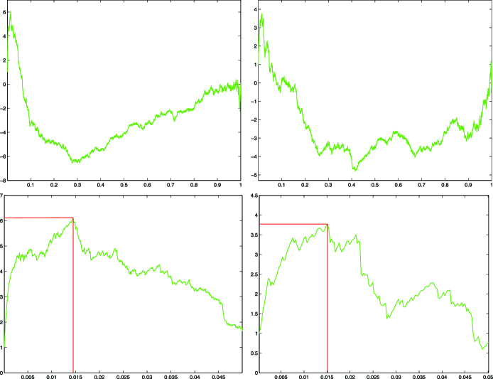
Figure 4: Top row: plot of feature scores $\mathrm{HC}_{N,i}$ versus $i/N$ for lung cancer data (left) and leukemia data (right). Bottom row: enlargements of plots in the top row.

3.1 Applications to Gene Microarray Data

We now apply the HCT classification rule to the two microarray data sets discussed earlier. Again, $Z_{j}$ is the standardized $Z$-score associated with the $j$th gene, using all samples in the training set $C$.

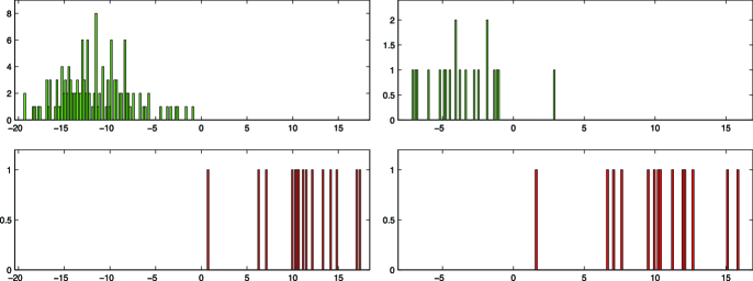
Figure 5: Top row: histogram of the test scores corresponding to class 1. Bottom row: class 2. Left column: lung cancer data. Right column: leukemia data.

First, we apply HC to $Z=(Z_{1},Z_{2},\ldots,Z_{p})^{\prime}$ to obtain the HC threshold; this will also determine how many features we keep for classification. The scores $\mathrm{HC}_{N,i}$ are displayed in Figure 4. For the lung cancer data, the maximizing index is $\hat{i}^{\mathrm{HC}}=182$, at which the HC score is $6.112$, and we retain all $182$ genes with the largest $Z$-scores (in absolute value) for classification (equivalently, a gene is retained if and only if the $Z$-score exceeds $\hat{t}_{p}^{\mathrm{HC}}=2.65$). For the leukemia data, $\hat{i}^{\mathrm{HC}}=54$, with HC score $3.771$ and the threshold $\hat{t}_{p}^{\mathrm{HC}}=2.68$.

Next, for each sample $X_{i}$ in the test set $D$, we calculate the HCT-based LDA score. Recall that for any $i\in C$, the data associated with the $i$th sample is $X_{i}=\{x_{ij}\}_{j=1}^{p}$. The HCT-based LDA score $\mathrm{lda}_{i}=\mathrm{lda}(X_{i})$ is given by

$$\mathrm{lda}_{i}=\sum_{j=1}^{p}w_{\mathrm{HC}}(j)\biggl{(}\frac{x_{ij}-\bar{x}_{j}}{s_{j}}\biggr{)},$$

where we recall $w_{\mathrm{HC}}(j)=\mathrm{sgn}(Z_{j})1\{|Z_{j}|\geq\hat{t}_{p}^{\mathrm{HC}}\}$, and $(\bar{x}_{j},s_{j},w_{\mathrm{HC}}(j))$ only depend on the training samples in $C$. The scores $\{\mathrm{lda}_{i}\}_{i=1}^{n}$ are displayed in Figure 5, where we normalized each score by a common factor of $1/\sqrt{\hat{i}^{\mathrm{HC}}}$ for clarity. The scores corresponding to class 1 are displayed in the top row in green (ADCA for lung cancer data and ALL for leukemia), and the scores for class 2 are displayed in the bottom row in red (the left column displays lung cancer data and the right column displays leukemia data). For lung cancer data, LDA–HCT correctly classifies each sample. For leukemia data, LDA–HCT correctly classifies each sample, with one exception: sample $29$ in the test set (number $67$ in the whole data set).

We employed these two data sets because they gave such a clear illustration. In our previous paper DJ08 , we considered each data in Dettling’s well-known compendium, which includes the colon cancer data and the prostate data. The results were largely as good as or better than other classifiers, many involving much fancier-sounding underlying principles.

3.2 Threshold Choice by HC: Applications to Biomarker Selection

Wehrens and Fannceschi Wehrens used HC thresholding for biomarker selection to analyze metabolomics data from spiked apples. They considered $P$-values that are calculated from Principal Component scores and reported a marked improvement in biomarker selection, compared to the standard selection obtained by existing practices. The paper concludes that HC thresholds can differ considerably from current practice, so it is no longer possible to blindly apply the selection thresholds used historically; the data-specific cutoff values provided by HC open the way to objective comparisons between biomarker selection methods, not biased by arbitrary habitual threshold choices.

3.3 Comparison to Other Classification Approaches

The LDA–HCT classifier is closely related to other threshold-based LDA feature selection rules: PAM by Tibshirani et al. Tibs and FAIR by Fan and Fan FanFan . HCT picks the threshold based on feature $Z$-scores by Higher Criticism, while the other methods set this threshold differently. For the same data sets we discussed earlier, the error rates for PAM and FAIR were reported in FanFan , Tibs ; as it turns out, LDA–HCT has smaller error rates.

Comparisons with some of the more popular “high-tech” classifiers (including Boosting Boosting , SVM SVM and Random Forests Breiman ) were reported in DJ08 . More complex methods usually need careful tuning to perform well, but HCT–LDA is very simple, both conceptually and computationally. When used on the ensemble of standard data sets published in Dettling, HCT–LDA happens to be minimax-regret optimal: it suffers the least performance loss, relative to the best method, across the ensemble.

Hall et al. Hall apply HC for classification in a different manner. They view HC as a goodness-of-fit diagnostic. Their method first uses the training vectors to obtain the empirical distributions of each class, and then uses HC to tell which of these distributions best fits each test vector. They classify each test vector using the best-fitting class distribution. While this rule is sensible, it turns out that in a formal asymptotic analysis using the rare/weak model, it is outperformed substantially by HCT–LDA.

3.4 Connection to Feature Selection by Controlling Feature-FDR

False Discovery Rate control methods offer a popular approach for feature selection. Fix $0<q<1$. $\mathrm{FDRT}_{q}$ selects features in a way so that

$$\mbox{feature-FDR}\equiv E\biggl{[}\frac{\#\{\mbox{Falsely selected features}\}}{\#\{\mbox{All selected features}\}}\biggr{]}\leq q.$$

In the simple setting considered in Section 3, this can be achieved by applying Benjamini–Hochberg’s FDR controlling method to all feature $P$-values. The approach appeals to the common belief that, in order to have optimal classification behavior, we should select features in a way so that the feature-FDR stays small.

However, such beliefs have theoretical support only when signals are rare/strong. In principle, the optimal $q$ associated with the optimal classification behavior should depend on the underlying distribution of the signals (e.g., sparsity and signal strength); and when signals are rare/weak, the optimal FDR level turns out to be much larger than $5\%$, and in some cases is close to $1$. In DJ09 , we studied the optimal level in an asymptotic rare/weak setting and derived the leading asymptotics of the optimal $\mathrm{FDR}$. In Section 6.2 below we give more detail.

In several papers Strimmer , Klaus , Klaus2 , Strimmer and collaborators compared the approach of feature selection by HCT with both that of control of the FDR and that of control of the False non-Discovery Rate (FNDR), analytically and also with synthetic data and several real data sets on cancer gene microarray. In their papers, they also compared the EBayes approach of Efron Efron , which presets an error rate threshold (say, $2.5\%$) and targets a threshold where the prediction error falls below the desired error rate. Their numerical studies confirm the points explained above: HCT adapts well to different sparsity level and signal strengths, while the methods of controlling FNDR and EBayes do not perform as well (in the misclassification sense); and HC typically selects more false features than other approaches. The goal of the HC feature selection, as we will see, is to optimize the classification error, not to control the FDR. In fact, Klaus , Table 2, found that HCT had the best classification performance for the cancer microarray data sets they investigated.

3.5 Feature Selection by HCT When Features Are Correlated

Above, we assumed the feature vector $X_{i}\sim N(Y_{i}\cdot\mu,I_{p})$ for $Y_{i}=\pm 1$. A natural generalization is to assume $X_{i}\sim N(Y_{i}\cdot\mu,\Sigma)$, where $\Sigma=\Sigma_{p,p}$ is a unknown covariance matrix. Two problems arise: how to estimate the precision matrix $\Omega=\Sigma^{-1}$ and how to incorporate the estimated precision matrix into the HCT classifier. In the latter, the key is to extend the idea of threshold choice by HCT to the setting where not only the features are correlated, but the covariance matrix is unknown and must be estimated.

The authors of HuangJin address the first problem by proposing Partial Correlation Screening (PCS) as a new row-wise approach to estimating the precision matrix. PCS starts by computing the $p\times p$ empirical scatter matrix $S=(1/n)\sum_{i=1}^{n}X_{i}X_{i}^{\prime}$. Assume the rows of $\Omega$ are relatively sparse. To estimate a row of $\Omega$, the algorithm only needs to access relatively few rows of $S$. For this reason, the method is able to cope with much larger $p$ (say, $p=10^{4}$) than existing approaches (e.g., Bickel and Levina BLT , glasso glasso , Neighborhood method MB and CLIME CaiLuo ). FanHC addresses the second problem by combining the ideas in Donoho and Jin DJ08 on threshold choices by HCT with those in Hall and Jin HJ on Innovated HC. This combination injects an estimate of $\Omega$ into the HCT classification method; it is asymptotically optimal if $\Omega$ is sufficiently sparse and we have a reasonably good estimate of $\Omega$ (e.g., CaiLuo ).

4 Testing Problems About a Large Covariance Matrix

In this section and the next, we briefly develop stylized applications of HC to settings which may seem initially far outside the original scope of the idea. In each case, HC requires merely the ability to compute a collection of $P$-values for a collection of statistics under an intersection null hypothesis. This allows us to easily obtain HC-tests in diverse settings.

Consider a data matrix $X=X_{n,p}$, where the rows of $X$ are i.i.d. samples from $N(0,\Sigma)$. We are interested in testing $\Sigma=I_{p}$ versus the hypothesis that $\Sigma$ contains a sub-structure. First, we consider the case where the substructure is a small-size clique. In Section 4.1, we approach the testing problem by applying HC to the whole body of pairwise empirical correlations and to the maximum row-wise correlation (for each variable, this is the maximum of each variable’s correlations with all other variables). Second, in Section 4.2, we consider the case where the matrix $\Sigma=I+H$ follows the so-called spiked covariance model John02 , a low-rank perturbation of the identity matrix. We apply HC to the eigenvalues of the empirical covariance matrix.

4.1 Detecting a Possible Clique in the Covariance Matrix

In this section, the global null hypothesis is $\Sigma=I_{p}$, while the alternative is that $\Sigma$ contains a small clique. Formally, $\Sigma$ can be written as $\Sigma=\Gamma\Sigma_{0}\Gamma^{\prime}$, where $\Gamma$ is a permutation matrix, and, for an integer $1\leq k<p$ and $a\in[0,1)$,

$$\Sigma_{0}(i,j)$$

(16)

$$\quad=\cases{1\{i=j\}+a\{i\neq j\},&$\max\{i,j\}\leq k,$\vspace*{2pt}\cr 1\{i=j\},&$\max\{i,j\}>k.$}$$

The parameter $a$ can take negative values as long as $\Sigma_{0}$ remains positive definite.

We suggest two different approaches for detecting the cliques using HC. In each of the two approaches, the key is to obtain $P$-values.

In the first approach, we obtain individual $P$-values from pairwise correlations. In detail, write the data matrix $X=X_{n,p}$ as

$$X=[x_{1},x_{2},\ldots,x_{p}].$$

The pairwise correlation between the $i$th and $j$th variable is

$$\rho_{ij}=\frac{(x_{i},x_{j})}{\|x_{i}\|\|x_{j}\|}.$$

Recall that $t_{k}(0)$ denotes the central Student’s $t$-distribution with $df=k$. The following lemma summarizes some basic properties of $\rho_{ij}$ Ruben .

Lemma 4.1.

Suppose $\Sigma=I_{p}$. If $i\neq j$, then for any $\rho\in(-1,1)$, $P(\rho_{ij}\geq\rho)=P(t_{n-1}(0)\geq\sqrt{n-1}\rho/\break\sqrt{1-\rho^{2}})$, Also, if $(i,j)\neq(k,\ell)$, then $\rho_{ij}$ and $\rho_{k\ell}$ are independent.

This says that the collection of random variables

$$\{\rho_{ij}\dvtx 1\leq i\leq j\leq p\}$$

are pairwise independent (but not jointly independent). It can be further shown that the correlation matrix between different $\rho_{ij}$ is very sparse, so a simple but reasonable approach is to apply OHC to $\{\rho_{ij}\dvtx 1\leq i\leq j\leq p\}$ directly. Numerically, the correlation between different $\rho_{ij}$ will not significantly affect the performance of OHC. On the other hand, since the correlation matrix between $\rho_{ij}$ can be calculated explicitly, a slightly more complicated method is to incorporate the correlation structures into HC, following the idea of Innovated HC InnovatedHC .

In the second approach, we obtain $P$-values from the maximum correlation in each row:

$$\rho_{i}^{*}=\max_{j\neq i}\rho_{ij},\quad 1\leq i\leq p.$$

Lemma 4.2.

Suppose $\Sigma=I_{p}$. For $1\leq i\leq p$ and $\rho\in(-1,1)$,

$$P\bigl{(}\rho_{i}^{*}\leq\rho\bigr{)} = \biggl{[}P\biggl{(}t_{n-1}(0)\leq\frac{\sqrt{(n-1)}\rho}{\sqrt{1-\rho^{2}}}\biggr{)}\biggr{]}^{p-1}$$

$$\equiv F_{p,n}(\rho).$$

For a proof, see Ruben , for example. Let $\pi_{i}^{*}=F_{p,n}(\rho_{i}^{*})$, so under the global null, $\pi_{i}^{*}\sim\mathrm{Unif}(0,1)$. We simply use these $P$-values in the standard HC framework.

We conducted a small-scale simulation as follows. Fix $(p,n)=(1000,500)$. We consider $5$ different combinations of $(k,a)$: $\{(1,0),(5,0.25),(15,0.2),\break(45,0.1),(135,0.05)\}$. For each combination, define $\Sigma_{0}$ as in (4.1). Note that, for the first combination, $\Sigma=I_{p}$. Also, since the OHC is permutation invariant, we take $\Gamma=I_{p}$ for simplicity so that $\Sigma=\Sigma_{0}$. For each $\Sigma$, we generate $n$ samples $X_{1},X_{2},\ldots,X_{n}$ from $N(0,\Sigma)$ and obtain $\rho_{ij}$ for all $1\leq i<j\leq p$.

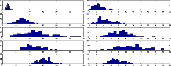
Figure 6: Simulated scores of OHC applied to pairwise correlations (left column) and maximum correlations (right column). The top panel represents the case of no cliques. The others represent cliques with various size and strength (introduced in the text). In comparison, OHC applied to maximum correlations has smaller power than OHC applied to pairwise correlations.

In the first approach, we sort all $N=p(p-1)/2$ different $P$-values $\{\pi_{ij}\dvtx 1\leq i<j\leq p\}$ in ascending order and write them as follows:

$$\pi_{(1)}<\pi_{(2)}<\cdots<\pi_{(N)},\quad N=p(p-1)/2.$$

We then apply the Orthodox Higher Criticism (OHC) and obtain the HC score

$$\mathrm{OHC}_{N}^{+} = \max_{i\dvtx 1/N\leq\pi_{(i)}\leq 1/2}\sqrt{N}\bigl{[}(i/N)-\pi_{(i)}\bigr{]}$$

$${}/\sqrt{\pi_{(i)}(1-\pi_{(i)})}.$$

In the second approach, we sort all $p$ different $P$-values $\pi_{j}^{*}$, $1\leq j\leq p$, in the ascending order and denote them by

$$\pi_{(1)}^{*}<\pi_{(2)}^{*}<\cdots<\pi_{(p)}^{*}.$$

We then apply the HC by (4.1), but with $\pi_{(i)}$ replaced by $\pi_{(i)}^{*}$.

The histograms of $\mathrm{OHC}_{N}^{+}$ based on $100$ repetitions are displayed in Figure 6, which suggests that OHC yields satisfactory detection. For all four types of cliques, the OHC applied in the second approach has smaller power in separation than that in the first approach.

4.2 Detecting Low-Rank Perturbations of the Identity Matrix

Now we test whether $\Sigma=I_{p}$ or instead we have a low-rank perturbation $\Sigma=I+H$, where the rank $r$ of $H$ is relatively small compared to $p$. Consider the spectral decomposition

$$\Sigma=Q\Lambda Q^{\prime},$$

where $Q$ is a $p\times p$ orthogonal matrix and $\Lambda$ is a diagonal matrix, with the first $r$ entries $1+h_{i}$, $h_{i}>0$, $1\leq i\leq r$, and other diagonal entries $1$. We assume the eigenbasis $Q$ is unknown to us. In a “typical” eigenbasis, the coordinates of $Q$ will be “uniformly small,” so that even if some of the eigenvalue excesses $h_{i}$ are nonzero $0$, the matrix $\Sigma$ can be close to the corresponding coordinates of $I_{p}$. Therefore, the pairwise covariances may be a very poor tool for diagnosing departure form the null.

Instead we work with the empirical spectral decomposition and apply HC to the sorted empirical eigenvalues. Denote the empirical covariance matrix by

$$S_{n}=(1/n)X^{\prime}X,$$

and let

$$\lambda_{1}>\lambda_{2}>\cdots>\lambda_{n}$$

be the (nonzero) eigenvalues of $S_{n}$ arranged in the descending order. The sorted eigenvalues play a role analogous to the sorted $P$-values in the earlier sections, since the perturbation of $I_{p}$ by a low-rank matrix $H$ will inflate a small fraction of the empirical eigenvalues, similar to the way the top few order statistics are inflated in the rare/weak model. We define our approximate $Z$-scores by standardizing each $\lambda_{i}$ using its mean and standard deviation under the null. The resulting $t$-like statistics, which we call the $\mathrm{eigenHC}$, are

$$\mathrm{eigenHC}_{n,i}=\frac{(\lambda_{i}-E_{0}[\lambda_{i}])}{\mathrm{\mathrm{SD}}_{0}(\lambda_{i})},\quad 1\leq i\leq p,$$ (18)

where $E_{0}[\lambda_{i}]$ and $\mathrm{SD}_{0}(\lambda_{i})$ are the mean and standard deviation of $\lambda_{i}$ evaluated under the null hypothesis $\Sigma=I_{p}$, respectively. Note that $E_{0}[\lambda_{i}]$ and $\mathrm{SD}_{0}(\lambda_{i})$ can be conveniently evaluated by Monte-Carlo simulations.

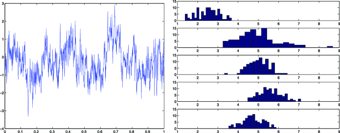
Figure 7: Left column: $x$-axis is $i/n$, $y$-axis is $\mathrm{eigenHC}_{n,i}$. Right column: simulated scores of $\mathrm{eigenHC}^{*}_{n}$. The top panel represents the unperturbed case. The others represent contamination with different ranks (introduced in text).

In Figure 7, we present a realization of $\{\mathrm{eigenHC}_{n,i}\dvtx\break 1\leq i\leq p\}$ in the case of $n=p=1000$. The figure looks vaguely similar to realizations of a normalized uniform empirical process, which suggests that the normalization in (18) makes sense. We consider the test statistic

$$\mathrm{eigenHC}_{n}^{*}=\max_{1\leq i\leq\alpha_{0}n}\{\mathrm{eigenHC}_{n,i}\},$$

where $\alpha_{0}$ is a tuning parameter we set here to $1/2$.

We conducted a small-scale simulation experiment, with $(p,n)=(1000,1000)$. For each of the $5$ different combinations of $(r,h)=(0,0),(5,1),\break(15,0.5),(45,0.2),(135,0.05)$, we let $\Lambda$ be the $p\times p$ diagonal matrix with first $r$ coordinates equal to $(1+h)$ and remaining coordinates all $1$. We then randomly generated a $p\times p$ orthogonal matrix $Q$ (according to the uniform measure on orthogonal matrices) and set

$$\Sigma=Q\Lambda Q^{\prime}.$$

Note that when $(r,h)=(0,0)$, $\Sigma=I_{p}$. Next, for each $\Sigma$, we generated data $X_{1},X_{2},\ldots,X_{n}\stackrel{{\scriptstyle\mathrm{i.i.d.}}}{{\sim}}\break N(0,\Sigma)$ and applied $\mathrm{eigenHC}_{n}^{*}$ to the synthetic data. Simulated results for $100$ such synthetic data sets are reported in Figure 7, illustrating that HC can yield satisfactory results even for small $r$ or $h$.

Testing hypotheses about large covariance matrices has received much attention in recent years. For example, Arias-Castro et al. Erycluster tested that the underlying covariance matrix is the identity versus the alternative where there is a small subset of correlated components. The correlated components may have a certain combinatorial structure known to the statistician. Butucea and Ingster Ingstermatrix consider testing the null model that the coordinates are i.i.d. $N(0,1)$ against a rare/weak model where a small fraction of them has significantly nonzero means. Muralidharan Muralidharan is also related; it adapts HC to test column dependences in gene microarray data.

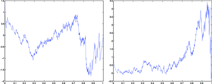
Figure 8: Plot of $\mathrm{pairHC}_{n,k}$ versus $k/n$ under the null (left) and under the alternative [right; $(\varepsilon,\tau,\rho)=(0.05,1,0.25)$]. $x$-axis is $k/n$ ($n=1000$).

5 Sparse Correlated Pairs Among Many Uncorrelated Pairs

Suppose we observe independent samples $(X_{i},Y_{i})$, $1\leq i\leq n$, from a bivariate distribution with zero means and unit variances, which is generally unknown to us. Under the null hypothesis, the $(X_{i})$ are independent of the corresponding $(Y_{i})$ (and each other); but under the alternative, for most pairs $(X_{i},Y_{i})$, independence holds, while for a small fraction $(X_{i},Y_{i})$, the two coordinates may be correlated and each may have an elevated mean. In short, some small collection of the pairs is correlated, unlike the bulk of the data.

Since the underlying distribution of the pairs $(X_{i},Y_{i})$ is unknown to us, we base our test statistics on ranks $(r_{i},s_{i})$ of the data $(X_{i},Y_{i})$. Our strategy is to compare the number of rank-pairs in the upper right corner to the number that would be expected under independence.

For $1\leq k\leq n$, let

$$S_{k} = \#\bigl{\{}1\leq i\leq n\dvtx\min\{r_{i},s_{i}\}\geq k\bigr{\}}$$

$$= \sum_{i=1}^{n}1\bigl{\{}\min\{r_{i},s_{i}\}\geq k\bigr{\}}.$$

Under the null, we have $P(\min\{r_{i},s_{i}\}\geq k)=P(r_{i}\geq k)P(s_{i}\geq k)=(1-k/n)^{2}$, so

$$E[S_{k}]=P(r_{i}\geq k)P(s_{i}\geq k)=n(1-k/n)^{2}$$

and

$$\operatorname{Var}(S_{k})=n\bigl{[}(1-k/n)^{2}\bigl{(}1-(1-k/n)^{2}\bigr{)}\bigr{]}.$$

Therefore, the HC idea applies as follows. Define

$$\mathrm{pairHC}_{n,k}=\sqrt{n}\frac{S_{k}/n-(1-k/n)^{2}}{\sqrt{(1-k/n)^{2}(1-(1-k/n)^{2})}}$$

and

$$\mathrm{pairHC}_{n}^{*}=\max_{(1-\alpha_{0})n\leq k\leq n}\mathrm{pairHC}_{n,k}.$$

Here, $\alpha_{0}$ is a tuning parameter and is set to $1/2$ below.

To illustrate this procedure, suppose that $(X_{i},Y_{i})$, $1\leq i\leq n$, are i.i.d. samples from a mixture of two bivariate normals

$$(1-\varepsilon)N(0,I_{2})+\varepsilon N(\tau{\mathbf{1}}_{2},\Sigma),$$

$${\mathbf{1}}_{2}=\pmatrix{1\cr 1},\quad\Sigma=\pmatrix{1&\rho\cr\rho&1},$$

where $(\varepsilon,\tau,\rho)$ are parameters. In Figure 8, we show a plot of $\mathrm{pairHC}_{n,k}$ for $n=1000$ and $k=1,2,\ldots,n$ under the null and under the alternative where $(\varepsilon,\tau,\rho)=(0.05,1,0.25)$.

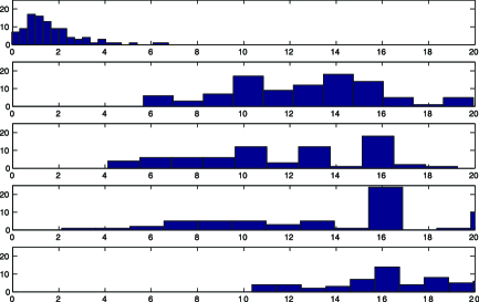
Figure 9: Simulated scores of $\mathrm{pairHC}_{n}^{*}$. The top panel represents the null case. The others represent the alternative cases with different $(\varepsilon,\tau,\rho)$, introduced in the text ($n=1000$).

We conducted a small simulation experiment as follows:

• Fix $n=1000$ and define $5$ different settings where $(\varepsilon,\tau,\rho)=(0,0,0)$, $(0.02,0,2.5)$, $(0.02,0.50,2)$,$(0.01,0.50,2.5)$ and $(0.01,0.25,3)$. Note that the first setting corresponds to the null case.

• Within each setting, conduct 100 Monte-Carlo repetitions, each time generating a synthetic data set with the given parameters and applying $\mathrm{pairHC}_{n}^{*}$.

The results are reported in Figure 9, which suggests that HC yields good separation even when the signals are relatively rare and weak.

6 Asymptotic Rare/Weak Model

In this section we review the rare/weak signal model and discuss the advantages of HC in this setting.

Return to the problem (3)–(2) of detecting a sparse Gaussian mixture. We introduce an asymptotic framework which we call the Asymptotic Rare/Weak (ARW) model. We consider a sequence of problems, indexed by the number $N$ of $P$-values (or $Z$-scores, or other base statistics); in the $N$th problem, we again consider mixtures $(1-\varepsilon)N(0,1)+\varepsilon N(\tau,1)$, but now we tie the behavior of $(\varepsilon,\tau)$ to $N$, in order to honor the spirit of the Rare/Weak situation. In detail, let $\vartheta\in(0,1)$ and set

$$\varepsilon=\varepsilon_{N}=N^{-\vartheta},$$

so that, as $N\rightarrow\infty$, the nonnull effects in $H_{1}^{(N)}$ become increasingly rare. To counter this effect, we let $\tau_{N}$ tend to $\infty$ slowly, so that the testing problem is (barely) solvable. In detail, fix $r>0$ and set

$$\tau_{N}=\sqrt{2r\log(N)}.$$

With these assumptions the Rare/Weak setting corresponds to $\vartheta>1/2$, rare enough that a shift in the overall mean is not detectable, and $r<1$, weak enough that a shift in the maximum observation is not detectable.

The key phenomenon in this model is a threshold for detectability. As a measure of detectability, consider the best possible sum of Types I and II errors of the optimal test. Then, there will be a precise threshold separating values of $(\vartheta,r)$, where the presence of the mixture is detectable from those where it is not detectable.

Let

$$\rho(\vartheta)=\cases{\vartheta-1/2,&$1/2<\vartheta\leq 3/4,$\vspace*{2pt}\cr\bigl{(}1-\sqrt{(1-\vartheta})\bigr{)}^{2},&$3/4<\vartheta<1.$}$$

When $r>\rho(\vartheta)$, the hypotheses separate asymptotically: the best sum of Types I and II errors tends to $0$ as $N$ tends to $\infty$. On the other hand, when $r<\rho(\vartheta)$, the sum of Types I and II errors of any test cannot get substantially smaller than $1$. The result was first proved by Ingster Ingster97 , Ingster99 , and then independently by Jin JinThesis , Jin04 .

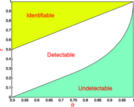
Figure 10: Phase diagram for the detection problem. The detection boundary separates the $\vartheta$-$r$ plane into the detectable region and the undetectable region. In the identifiable region, it is not only able to reliably tell the existence of nonzero coordinates, but also possible to identify individual nonzero coordinates.

In other words, in the two-dimensional $\vartheta$-$r$ phase space, the curve $r=\rho(\vartheta)$ separates the bounded region $\{(\vartheta,r)\dvtx 1/2<\vartheta<1,0<r<1\}$ into two separate subregions, the detectable region and the undetectable region. For $(\vartheta,r)$ in the interior of the detectable region, two hypotheses separate asymptotically and it is possible to separate them. For $(\vartheta,r)$ in the undetectable region, two hypotheses merge asymptotically, and it is impossible to separate them. Hence, the phase diagram splits into two “phases”; see Figure 10 for illustration.

Fix $(\vartheta,r)$ in the detectable region. Suppose we reject $H_{0}^{(N)}$ if and only

$$\mathrm{HC}_{N}^{*}\geq h(N,\alpha_{N}),$$

where $\alpha_{N}$ tends to $0$ slowly enough so that $h(N,\break\alpha_{N})=O(\sqrt{2\log\log(N)})$. Then when $H_{1}^{(N)}$ can be detected by the optimal test, HC also detects it, as $N\rightarrow\infty$.

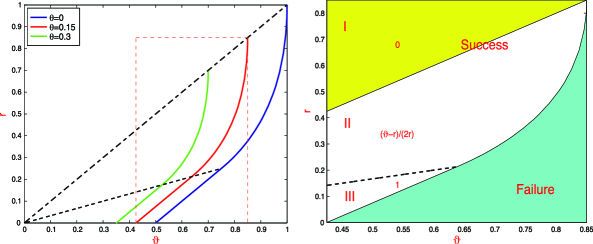
Figure 11: Left: curves $r=\rho_{\theta}(\vartheta)$ for $\theta=0,0.15,0.3$. Two dashed black lines are $r=\vartheta$ and $r=\vartheta/3$, respectively. For $\theta=0.15$, the most interesting region is represented by the rectangular box. Right: enlargement of the rectangular box. The curve $r=\rho_{\theta}(\vartheta)$ ($\theta=0.15$) splits the box into two subregions: Failure (cyan) and Success (white and yellow). The two lines $r=\vartheta$ and $r=\vartheta/3$ further split Region of Success into three subregions, I, II and III, where the leading terms of $q^{\mathrm{ideal}}(\vartheta,r,p)$ in (6.2) are shown. In the yellow region, it is not only possible to have successful classifications, but is also possible to separate useful features from useless ones.

Since HC can be applied without knowing the underlying parameter $(\vartheta,r)$, we say HC is optimally adaptive. HC thus has an advantage over the Neyman–Pearson likelihood ratio test (LRT), which requires precise information about the underlying ARW parameters. The HC approach can be applied much more generally; it is only for theoretical analysis that we focus on the narrow ARW model.

A similar phase diagram holds in a classification problem considered in Section 3, provided that we calibrate the parameters appropriately. Consider a sequence of classification problems indexed by $(n,p)$, where $n$ is the number of observations and $p$ the number of features available to the classifier. Suppose that two classes are equally likely so that $P(Y_{i}=1)=P(Y_{i}=-1)=1/2$ for all $1\leq i\leq n$. For $Z$ in (12), recall that $Z\sim N(\sqrt{n}\mu,I_{p})$. We calibrate with

$$\sqrt{n}\mu(j)\stackrel{{\scriptstyle\mathrm{i.i.d.}}}{{\sim}}(1-\varepsilon)\nu_{0}+\varepsilon\nu_{\tau},$$

where $\nu_{a}$ denotes the point mass at $a$. Similarly, we use an ARW model, where we fix $(\vartheta,r,\theta)\in(0,1)^{3}$ and let

$$\varepsilon = \varepsilon_{p}=p^{-\vartheta},\quad\tau=\tau_{p}=\sqrt{2r\log(p)},$$

$$n = n_{p}=p^{\theta}.$$

Note that when $p\rightarrow\infty$, $n_{p}$ grows with $p$, but is still much smaller than $p$. We call such growth regular growth. The results below hold for other types of growth of $n$; see Jin JinPNAS , for example.

It turns out that there is a similar phase diagram associated with the classification problem. Toward this end, define

$$\rho_{\theta}(\vartheta)=(1-\theta)\rho\biggl{(}\frac{\vartheta}{1-\theta}\biggr{)},\quad 0<\vartheta<(1-\theta).$$

Fix $\theta\in(0,1)$. In the two-dimensional phase space, the most interesting region for $(\vartheta,r)$ is the rectangular region $\{(\vartheta,r)\dvtx 0<\vartheta,r<(1-\theta)\}$. The region partitions into two subregions:

• (Region of success). If $r>\rho_{\theta}(\vartheta)$, then the HC threshold $\hat{t}_{p}^{\mathrm{HC}}/t_{p}^{\mathrm{ideal}}\rightarrow 1$ in probability; $t_{p}^{\mathrm{ideal}}$ is the ideal threshold that one would choose if the underlying parameters $(\vartheta,r)$ are known. Note that HCT is driven by data, without the knowledge of $(\vartheta,r)$. Also, the classification error of an HCT-trained classification rule tends to $0$ as $p\rightarrow\infty$.

• (Region of failure). When $r<\rho_{\theta}(\vartheta)$, the classification error of any trained classification rule tends to $1/2$, as $p\rightarrow\infty$.

See Figure 11. The above includes the case where $n_{p}\rightarrow\infty$ but $n_{p}/p^{a}\rightarrow 0$ for any fixed $a>0$ as the special case of $\theta=0$. See more discussion in DJ08 , JinPNAS , DJ09 . Ingster et al. IPT derived independently the classification boundary, in a broader setting than that in DJ08 , JinPNAS , DJ09 , but they did not discuss HC.

The conceptual advantage of HC lies in its ability to perform optimally under the ARW framework—without needing to know the underlying ARW parameters: HC is a data-driven nonparametric statistic that is not tied to the idealized model we discussed here, and yet works well in this model.

The phase diagrams above are for settings where the test statistics or measured features $X_{i}$ are independent normals with unit variances (the normal means may be different). In more complicated settings, how to derive the phase diagrams is an interesting but nontrivial problem. Delaigle et al. Robustness studied the problem of detecting sparse mixtures by extending models (3)–(2) to a setting where $X_{i}$ are the Student’s $t$-scores based on (possibly) non-Gaussian data, where the marginal density of $X_{i}$ is unknown but is approximately normal. Fan et al. FanHC extended the classification problem considered in Section 3 to a setting where the measured features are correlated; the covariance matrix is unknown and must be estimated. In general, the approximation errors (either in the underlying marginal density or the estimated covariance matrix) have a negligible effect on the phase diagrams when the true effects are sufficiently sparse and a nonnegligible yet subtle effect when the true effects are moderately sparse; see Robustness , FanHC .

6.1 Phase Diagram in the Nonasymptotic Context

The phase diagrams depict an asymptotic situation; it is natural to ask how they behave for finite $N$. This has been studied in DJ09 , Figure 4, Sun Sun , Blomberg Blomberg and Rohban . In principle, for finite $N$, we would not experience “perfectly sharp” phase transition as visualized in Figures 10 and 11. However, numeric studies reveal that, for reasonably large $N$, the transition zone between the region where inference can be rather satisfactory and the region where inference is nearly impossible is comparably narrow, increasingly so as $N$ increases. Sun Sun used such ideas to study a GWAS on Parkinson’s disease, and argued that standard designs for GWAS are inefficient in many cases. Xie Xie and Wu Meihua used the phase diagram as a framework for sample size and power calculations.

6.2 Phase Diagram for FDR-Controlling Methods

Continuing the discussion in Section 3.4, we investigate the optimal FDR control parameter $q$ in the rare/weak setting. Suppose we select features by applying Benjamini–Hochberg’s FDR-controlling method to the ARW. The “ideal” FDR control parameter $q^{\mathrm{ideal}}(\vartheta,r,p)$ is the feature-FDR associated with $t_{p}^{\mathrm{ideal}}$ (i.e., we have a discovery if and only if the feature $Z$-score exceeds $t_{p}^{\mathrm{ideal}}$ in magnitude). In Donoho and Jin DJ09 , it is shown that, as $p\rightarrow\infty$,

$$q^{\mathrm{ideal}}(\vartheta,r,p)$$

$$\quad=\cases{o(1),&$r>\vartheta,$\vspace*{2pt}\cr\displaystyle\frac{\vartheta-r}{2r}+o(1),&$\vartheta/3<r<\vartheta,$\vspace*{2pt}\cr 1-o(1),&$\rho_{\theta}(\vartheta)<r<\vartheta/3,$}$$

which gives an interesting 3-phase structure: see Regions I, II, III in Figure 11. Somewhat surprisingly, the optimal FDR is very close to $1$ in one of the three phases (i.e., Region III); in this phase, to obtain optimal classification behavior, we set the feature selection threshold very low so that we include most of the useful features; but when we do this, we necessarily include many useless features, which dominate in numbers among all selected features. Similar comments apply when replacing Benjamini–Hochberg’s FDR control by the local FDR (Lfdr) approach of Efron Efron ; see DJ09 for details.

6.3 Phase Diagrams in Other Rare/Weak Settings

Phase diagrams offer a new criterion for measuring performance in multiple testing in the rare/weak effects model.

This framework is useful in many other settings. Consider a linear regression model $Y=X\beta+z$, $z\sim N(0,I_{n})$, where $X=X_{n,p}$ and $p\geq n$. The signals in the coefficient vector $\beta$ are rare and weak, and the goal is variable selection (different from that in Section 2.10). In a series of papers GJW , JiJin , JZZ , Ke , we use the Hamming error as the loss function for variable selection and study phase diagrams in settings where the matrices $X$ get increasingly “bad” so the problem get increasingly harder. These studies propose several new variable selection procedures, including UPS JiJin , Graphlet Screening JZZ and CASE Ke . The study is closely related to Donoho on Compressed Sensing.

References JW1 , JW2 present ARW phase diagrams for sparse spectral clustering, and Fienberg presents phase diagrams for computer privacy and confidentiality.

References

- (1) {barticle}[auto:parserefs-M02] \bauthor\bsnmAddario-Berry, \bfnmL.\binitsL., \bauthor\bsnmBroutin, \bfnmN.\binitsN., \bauthor\bsnmDevroye, \bfnmL.\binitsL. and \bauthor\bsnmLugosi, \bfnmG.\binitsG. (\byear2010). \btitleOn combinatorial testing problems. \bjournalAnn. Statist. \bvolume38 \bpages3063–3092. \bidmr=2722464 \bptokimsref \endbibitem
- (2) {barticle}[auto:parserefs-M02] \bauthor\bsnmAhdesmäki, \bfnmM.\binitsM. and \bauthor\bsnmStrimmer, \bfnmK.\binitsK. (\byear2010). \btitleFeature selection in omics prediction problems using cat scores and false nondiscovery rate control. \bjournalAnn. Appl. Stat. \bvolume4 \bpages503–519. \bidmr=2758182 \bptokimsref \endbibitem
- (3) {bmisc}[auto:parserefs-M02] \bauthor\bsnmAnderson, \bfnmC.\binitsC. (\byear2008). \bhowpublishedThe end of theory: The data deluge makes the scientific method obsolete. Wired Magazine 16.07 June 23 2008. \bptokimsref\endbibitem
- (4) {barticle}[auto:parserefs-M02] \bauthor\bsnmAnderson, \bfnmT. W.\binitsT. W. and \bauthor\bsnmDarling, \bfnmD. A.\binitsD. A. (\byear1952). \btitleAsymptotic theory of certain “goodness of fit” criteria based on stochastic processes. \bjournalAnn. Math. Statist. \bvolume23 \bpages193–212. \bidmr=0050238 \bptokimsref \endbibitem
- (5) {barticle}[auto:parserefs-M02] \bauthor\bsnmArias-Castro, \bfnmE.\binitsE., \bauthor\bsnmCandès, \bfnmE.\binitsE. and \bauthor\bsnmDurand, \bfnmA.\binitsA. (\byear2011). \btitleDetection of an anomalous cluster in a network. \bjournalAnn. Statist. \bvolume39 \bpages278–304. \bidmr=2797847 \bptokimsref \endbibitem
- (6) {barticle}[auto:parserefs-M02] \bauthor\bsnmArias-Castro, \bfnmE.\binitsE., \bauthor\bsnmCandès, \bfnmE.\binitsE. and \bauthor\bsnmPlan, \bfnmY.\binitsY. (\byear2011). \btitleGlobal testing under sparse alternatives: ANOVA, multiple comparisons and the higher criticism. \bjournalAnn. Statist. \bvolume39 \bpages2533–2556. \bidmr=2906877 \bptokimsref \endbibitem
- (7) {bmisc}[auto:parserefs-M02] \bauthor\bsnmArias-Castro, \bfnmE.\binitsE. and \bauthor\bsnmWang, \bfnmM.\binitsM. (\byear2013). \bhowpublishedDistribution free tests for sparse heterogeneous mixtures. Available at \arxivurlarXiv:1308.0346. \bptokimsref\endbibitem
- (8) {barticle}[auto:parserefs-M02] \bauthor\bsnmBalabdaoui, \bfnmF.\binitsF., \bauthor\bsnmJankowski, \bfnmH.\binitsH., \bauthor\bsnmPavlides, \bfnmM.\binitsM., \bauthor\bsnmSeregin, \bfnmA.\binitsA. and \bauthor\bsnmWellner, \bfnmJ.\binitsJ. (\byear2011). \btitleOn the Grenander estimator at zero. \bjournalStatist. Sinica \bvolume21 \bpages873–899. \bidmr=2829859 \bptokimsref \endbibitem
- (9) {barticle}[auto:parserefs-M02] \bauthor\bsnmBenjamini, \bfnmY.\binitsY. (\byear2010). \btitleDiscovering the false discovery rate. \bjournalJ. R. Stat. Soc. Ser. B. Stat. Methodol. \bvolume72 \bpages405–416. \bidmr=2758522 \bptokimsref \endbibitem
- (10) {barticle}[auto:parserefs-M02] \bauthor\bsnmBenjamini, \bfnmY.\binitsY. and \bauthor\bsnmHochberg, \bfnmY.\binitsY. (\byear1995). \btitleControlling the false discovery rate: A practical and powerful approach to multiple testing. \bjournalJ. R. Stat. Soc. Ser. B. Stat. Methodol. \bvolume57 \bpages289–300. \bidmr=1325392 \bptokimsref \endbibitem
- (11) {barticle}[auto:parserefs-M02] \bauthor\bsnmBennett, \bfnmM. F.\binitsM. F., \bauthor\bsnmMelatos, \bfnmA.\binitsA., \bauthor\bsnmDelaigle, \bfnmA.\binitsA. and \bauthor\bsnmHall, \bfnmP.\binitsP. (\byear2012). \btitleReanalysis of -statistics gravitational-wave search with the higher criticism statistics. \bjournalAstrophys. J. \bvolume766 \bpages1–10. \bptokimsref\endbibitem
- (12) {barticle}[auto:parserefs-M02] \bauthor\bsnmBerk, \bfnmR. H.\binitsR. H. and \bauthor\bsnmJones, \bfnmD. H.\binitsD. H. (\byear1979). \btitleGoodness-of-fit test statistics that dominates the Kolmogorov statistic. \bjournalZ. Wahrsch. Verw. Geb. \bvolume47 \bpages47–59. \bptokimsref\endbibitem
- (13) {barticle}[auto:parserefs-M02] \bauthor\bsnmBickel, \bfnmP.\binitsP. and \bauthor\bsnmLevina, \bfnmE.\binitsE. (\byear2008). \btitleRegularized estimation of large covariance matrices. \bjournalAnn. Statist. \bvolume36 \bpages199–227. \bidmr=2387969 \bptokimsref \endbibitem
- (14) {bmisc}[auto:parserefs-M02] \bauthor\bsnmBlomberg, \bfnmN.\binitsN. (\byear2012). \bhowpublishedHigher criticism testing for signal detection in rare and weak models. Master thesis, KTH Royal Institute of Technology, Stockholm, Sweden. \bptokimsref\endbibitem
- (15) {bmisc}[auto:parserefs-M02] \bauthor\bsnmBogdan, \bfnmM.\binitsM., \bauthor\bsnmGhosh, \bfnmJ.\binitsJ. and \bauthor\bsnmTokdar, \bfnmT.\binitsT. (\byear2008). \bhowpublishedA comparison of the Benjamini–Hochberg procedure with some Bayesian rules for multiple testing. In Beyond Parametrics in Interdisciplinary Research: Festschrift in Honor of Professor Pranab K. Sen 1 211–230. IMS, Beachwood, OH. \bidmr=2462208 \bptokimsref \endbibitem
- (16) {barticle}[auto:parserefs-M02] \bauthor\bsnmBogdan, \bfnmM.\binitsM., \bauthor\bsnmChakrabarti, \bfnmA.\binitsA., \bauthor\bsnmFrommlet, \bfnmF.\binitsF. and \bauthor\bsnmGhosh, \bfnmJ.\binitsJ. (\byear2011). \btitleAsymptotic Bayes-optimality under sparsity of some multiple testing procedures. \bjournalAnn. Statist. \bvolume39 \bpages1551–1579. \bidmr=2850212 \bptokimsref \endbibitem
- (17) {barticle}[auto:parserefs-M02] \bauthor\bsnmBox, \bfnmM.\binitsM. and \bauthor\bsnmMeyer, \bfnmD.\binitsD. (\byear1986). \btitleAn analysis for unreplicated fractional factorials. \bjournalTechnometrics \bvolume28 \bpages11–18. \bidmr=0824728 \bptokimsref \endbibitem
- (18) {barticle}[auto:parserefs-M02] \bauthor\bsnmBreiman, \bfnmL.\binitsL. (\byear2001). \btitleRandom forests. \bjournalMach. Learn. \bvolume24 \bpages5–32. \bptokimsref\endbibitem
- (19) {barticle}[auto:parserefs-M02] \bauthor\bsnmBurges, \bfnmC.\binitsC. (\byear1998). \btitleA tutorial on support vector machines for pattern recognition. \bjournalData Min. Knowl. Discov. \bvolume2 \bpages121–167. \bptokimsref\endbibitem
- (20) {barticle}[auto:parserefs-M02] \bauthor\bsnmButucea, \bfnmC.\binitsC. and \bauthor\bsnmIngster, \bfnmY. I.\binitsY. I. (\byear2013). \btitleDetection of a sparse submatrix of a high-dimensional noisy matrix. \bjournalBernoulli \bvolume19 \bpages2652–2688. \bidmr=3160567 \bptokimsref \endbibitem
- (21) {barticle}[auto:parserefs-M02] \bauthor\bsnmCai, \bfnmT.\binitsT., \bauthor\bsnmJeng, \bfnmJ.\binitsJ. and \bauthor\bsnmJin, \bfnmJ.\binitsJ. (\byear2011). \btitleDetecting sparse heterogeneous and heteroscedastic mixtures. \bjournalJ. R. Stat. Soc. Ser. B. Stat. Methodol. \bvolume73 \bpages629–662. \bidmr=2867452 \bptokimsref \endbibitem
- (22) {barticle}[auto:parserefs-M02] \bauthor\bsnmCai, \bfnmT.\binitsT. and \bauthor\bsnmJin, \bfnmJ.\binitsJ. (\byear2010). \btitleOptimal rate of convergence of estimating the null density and the proportion of non-null effects in large-scale multiple testing. \bjournalAnn. Statist. \bvolume38 \bpages100–145. \bidmr=2589318 \bptokimsref \endbibitem
- (23) {barticle}[auto:parserefs-M02] \bauthor\bsnmCai, \bfnmT.\binitsT., \bauthor\bsnmJin, \bfnmJ.\binitsJ. and \bauthor\bsnmLow, \bfnmM.\binitsM. (\byear2007). \btitleEstimation and confidence sets for sparse normal mixtures. \bjournalAnn. Statist. \bvolume35 \bpages2421–2449. \bidmr=2382653 \bptokimsref \endbibitem
- (24) {barticle}[auto:parserefs-M02] \bauthor\bsnmCai, \bfnmT.\binitsT., \bauthor\bsnmLiu, \bfnmW.\binitsW. and \bauthor\bsnmLuo, \bfnmX.\binitsX. (\byear2010). \btitleA constrained minimization approach to sparse precision matrix estimation. \bjournalJ. Amer. Statist. Assoc. \bvolume106 \bpages594–607. \bidmr=2847973 \bptokimsref \endbibitem
- (25) {barticle}[auto:parserefs-M02] \bauthor\bsnmCai, \bfnmT.\binitsT. and \bauthor\bsnmWu, \bfnmY.\binitsY. (\byear2014). \btitleOptimal detection of sparse mixtures against a given null distribution. \bjournalIEEE Trans. Inform. Theory \bvolume60 \bpages2217–2232. \bidmr=3181520 \bptokimsref \endbibitem
- (26) {barticle}[auto:parserefs-M02] \bauthor\bsnmCayon, \bfnmL.\binitsL., \bauthor\bsnmBanday, \bfnmA. J.\binitsA. J. \betalet al. (\byear2006). \btitleNo higher criticism of the Bianchi-corrected Wilkinson microwave anisotropy probe data. \bjournalMon. Not. Roy. Astron. Soc. \bvolume369 \bpages598–602. \bptokimsref\endbibitem
- (27) {barticle}[auto:parserefs-M02] \bauthor\bsnmCayon, \bfnmL.\binitsL., \bauthor\bsnmJin, \bfnmJ.\binitsJ. and \bauthor\bsnmTreaster, \bfnmA.\binitsA. (\byear2004). \btitleHigher criticism statistic: Detecting and identifying non-Gaussianity in the WMAP first year data. \bjournalMon. Not. Roy. Astron. Soc. \bvolume362 \bpages826–832. \bptokimsref\endbibitem
- (28) {bmisc}[auto:parserefs-M02] \bauthor\bsnmCharbonnier, \bfnmG.\binitsG. (\byear2012). \bhowpublishedInference of gene regulatory network from non independently and identically distributed transcriptomic data. Ph.D. thesis, Univ. d’Évry Val-d’Essonne, France. \bptokimsref\endbibitem
- (29) {barticle}[auto:parserefs-M02] \bauthor\bsnmCruz, \bfnmM.\binitsM., \bauthor\bsnmCayon, \bfnmL.\binitsL., \bauthor\bsnmMartinez-Gonzalez, \bfnmE.\binitsE., \bauthor\bsnmVielva, \bfnmP.\binitsP. and \bauthor\bsnmJin, \bfnmJ.\binitsJ. (\byear2007). \btitleThe non-Gaussian cold spot in the 3 year Wilkinson Microwave Anisotropy Probe data. \bjournalAstrophys. J. \bvolume655 \bpages11–20. \bptokimsref\endbibitem
- (30) {barticle}[auto:parserefs-M02] \bauthor\bsnmDai, \bfnmH.\binitsH., \bauthor\bsnmCharnigo, \bfnmR.\binitsR., \bauthor\bsnmSrivastava, \bfnmT.\binitsT., \bauthor\bsnmTalebizadeh, \bfnmZ.\binitsZ. and \bauthor\bsnmQing, \bfnmS.\binitsS. (\byear2012). \btitleIntegrating -values for genetic and genomic data analysis. \bjournalJ. Biom. Biostat. \bvolume2012 \bpages3–7. \bptokimsref\endbibitem
- (31) {barticle}[auto:parserefs-M02] \bauthor\bsnmDasgupta, \bfnmA.\binitsA., \bauthor\bsnmLahiri, \bfnmS.\binitsS. and \bauthor\bsnmStoyanov, \bfnmJ.\binitsJ. (\byear2014). \btitleSharp fixed bounds and asymptotic expansions for the means and the median of a Gaussian sample maximum, and applications to Donoho–Jin model. \bjournalStat. Methodol. \bvolume20 \bpages40–62. \bidmr=3205720 \bptokimsref \endbibitem
- (32) {barticle}[pbm] \bauthor\bparticlede \bsnmUña-Alvarez, \bfnmJacobo\binitsJ. (\byear2012). \btitleThe Beta-Binomial SGoF method for multiple dependent tests. \bjournalStat. Appl. Genet. Mol. Biol. \bvolume11 \bpages1544–6115. \bidissn=1544-6115, pmid=22611594, mr=2934896 \bptokimsref \endbibitem
- (33) {bincollection}[auto:parserefs-M02] \bauthor\bsnmDelaigle, \bfnmA.\binitsA. and \bauthor\bsnmHall, \bfnmP.\binitsP. (\byear2009). \btitleHigher criticism in the context of unknown distribution, non-independence and classification. In \bbooktitlePerspectives in Mathematical Sciences I: Probability and Statistics (\beditor\bfnmN.\binitsN. \bsnmSastry, \beditor\bfnmM.\binitsM. \bsnmDelampady, \beditor\bfnmB.\binitsB. \bsnmRajeev and \beditor\bfnmT. S. S. R. K.\binitsT. S. S. R. K. \bsnmRao, eds.) \bpages109–138. \bpublisherWorld Scientific. \bidmr=2581742 \bptokimsref \endbibitem
- (34) {barticle}[auto:parserefs-M02] \bauthor\bsnmDelaigle, \bfnmA.\binitsA., \bauthor\bsnmHall, \bfnmJ.\binitsJ. and \bauthor\bsnmJin, \bfnmJ.\binitsJ. (\byear2011). \btitleRobustness and accuracy of methods for high dimensional data analysis based on Student’s t statistic. \bjournalJ. R. Stat. Soc. Ser. B. Stat. Methodol. \bvolume73 \bpages283–301. \bidmr=2815777 \bptokimsref \endbibitem
- (35) {barticle}[pbm] \bauthor\bsnmDettling, \bfnmMarcel\binitsM. (\byear2004). \btitleBagBoosting for tumor classification with gene expression data. \bjournalBioinformatics \bvolume20 \bpages3583–3593. \biddoi=10.1093/bioinformatics/bth447, issn=1367-4803, pii=bth447, pmid=15466910 \bptokimsref\endbibitem
- (36) {barticle}[pbm] \bauthor\bsnmDettling, \bfnmMarcel\binitsM. and \bauthor\bsnmBühlmann, \bfnmPeter\binitsP. (\byear2003). \btitleBoosting for tumor classification with gene expression data. \bjournalBioinformatics \bvolume19 \bpages1061–1069. \bidissn=1367-4803, pmid=12801866 \bptokimsref\endbibitem
- (37) {barticle}[pbm] \bauthor\bparticleDe la \bsnmCruz, \bfnmOmar\binitsO., \bauthor\bsnmWen, \bfnmXiaoquan\binitsX., \bauthor\bsnmKe, \bfnmBaoguan\binitsB., \bauthor\bsnmSong, \bfnmMinsun\binitsM. and \bauthor\bsnmNicolae, \bfnmDan L.\binitsD. L. (\byear2010). \btitleGene, region and pathway level analyses in whole-genome studies. \bjournalGenet. Epidemiol. \bvolume34 \bpages222–231. \biddoi=10.1002/gepi.20452, issn=1098-2272, mid=NIHMS583784, pmcid=4061611, pmid=20013942 \bptokimsref\endbibitem
- (38) {barticle}[auto:parserefs-M02] \bauthor\bsnmDonoho, \bfnmD.\binitsD. (\byear2006). \btitleCompressed sensing. \bjournalIEEE Trans. Inform. Theory \bvolume52 \bpages1289–1306. \bidmr=2241189 \bptokimsref \endbibitem
- (39) {barticle}[auto:parserefs-M02] \bauthor\bsnmDonoho, \bfnmD.\binitsD. and \bauthor\bsnmJin, \bfnmJ.\binitsJ. (\byear2004). \btitleHigher criticism for detecting sparse heterogeneous mixtures. \bjournalAnn. Statist. \bvolume32 \bpages962–994. \bidmr=2065195 \bptokimsref \endbibitem
- (40) {barticle}[pbm] \bauthor\bsnmDonoho, \bfnmDavid\binitsD. and \bauthor\bsnmJin, \bfnmJiashun\binitsJ. (\byear2008). \btitleHigher criticism thresholding: Optimal feature selection when useful features are rare and weak. \bjournalProc. Natl. Acad. Sci. USA \bvolume105 \bpages14790–14795. \biddoi=10.1073/pnas.0807471105, issn=1091-6490, pii=0807471105, pmcid=2553037, pmid=18815365 \bptokimsref\endbibitem
- (41) {barticle}[auto:parserefs-M02] \bauthor\bsnmDonoho, \bfnmD.\binitsD. and \bauthor\bsnmJin, \bfnmJ.\binitsJ. (\byear2009). \btitleFeature selection by Higher Criticism thresholding: Optimal phase diagram. \bjournalPhilos. Trans. R. Soc. Lond. Ser. A Math. Phys. Eng. Sci. \bvolume367 \bpages4449–4470. \bidmr=2546396 \bptokimsref \endbibitem
- (42) {barticle}[auto:parserefs-M02] \bauthor\bsnmEfron, \bfnmB.\binitsB. (\byear2004). \btitleLarge-scale simultaneous hypothesis testing: The choice of a null hypothesis. \bjournalJ. Amer. Statist. Assoc. \bvolume99 \bpages96–104. \bidmr=2054289 \bptokimsref \endbibitem
- (43) {bbook}[auto:parserefs-M02] \bauthor\bsnmEfron, \bfnmB.\binitsB. (\byear2011). \btitleLarge-Scale Inference: Empirical Bayes Methods for Estimation, Testing, and Prediction. \bpublisherCambridge Univ. Press, \blocationCambridge. \bidmr=2724758 \bptokimsref \endbibitem
- (44) {barticle}[auto:parserefs-M02] \bauthor\bsnmEfron, \bfnmB.\binitsB., \bauthor\bsnmTibshirani, \bfnmR.\binitsR., \bauthor\bsnmStorey, \bfnmJ.\binitsJ. and \bauthor\bsnmTusher, \bfnmV.\binitsV. (\byear2001). \btitleEmpirical Bayes analysis of a microarray experiment. \bjournalJ. Amer. Statist. Assoc. \bvolume99 \bpages96–104. \bidmr=1946571 \bptokimsref \endbibitem
- (45) {barticle}[auto:parserefs-M02] \bauthor\bsnmEl-Fishawy, \bfnmP.\binitsP. (\byear2013). \btitleCommon disease-common variant hypothesis. \bjournalEncyclopedia of Autism Spectral Disorder \bpages719–720. \bptokimsref\endbibitem
- (46) {barticle}[auto:parserefs-M02] \bauthor\bsnmFan, \bfnmJ.\binitsJ. and \bauthor\bsnmFan, \bfnmY.\binitsY. (\byear2008). \btitleHigh dimensional classification using features annealed independence rules. \bjournalAnn. Statist. \bvolume36 \bpages2605–2637. \bidmr=2485009 \bptokimsref \endbibitem
- (47) {barticle}[auto:parserefs-M02] \bauthor\bsnmFan, \bfnmY.\binitsY., \bauthor\bsnmJin, \bfnmJ.\binitsJ. and \bauthor\bsnmYao, \bfnmZ.\binitsZ. (\byear2013). \btitleOptimal feature selection by higher criticism in sparse Gaussian graphic model. \bjournalAnn. Statist. \bvolume41 \bpages2537–2571. \bptokimsref\endbibitem
- (48) {barticle}[auto:parserefs-M02] \bauthor\bsnmFienberg, \bfnmS.\binitsS. and \bauthor\bsnmJin, \bfnmJ.\binitsJ. (\byear2012). \btitlePrivacy-preserving data sharing in high dimensional regression and classification settings. \bjournalJ. Privacy and Confidentiality \bvolume4 \bnoteArticle 10. \bptokimsref\endbibitem
- (49) {barticle}[pbm] \bauthor\bsnmFriedman, \bfnmJerome\binitsJ., \bauthor\bsnmHastie, \bfnmTrevor\binitsT. and \bauthor\bsnmTibshirani, \bfnmRobert\binitsR. (\byear2008). \btitleSparse inverse covariance estimation with the graphical lasso. \bjournalBiostatistics \bvolume9 \bpages432–441. \biddoi=10.1093/biostatistics/kxm045, issn=1468-4357, mid=NIHMS248717, pii=kxm045, pmcid=3019769, pmid=18079126 \bptnotecheck year \bptokimsref\endbibitem
- (50) {bmisc}[auto:parserefs-M02] \bauthor\bsnmGayraud, \bfnmG.\binitsG. and \bauthor\bsnmIngster, \bfnmY. I.\binitsY. I. (\byear2011). \bhowpublishedDetection of sparse variable functions. Available at \arxivurlarXiv:1011.6369. \bptokimsref\endbibitem
- (51) {barticle}[auto:parserefs-M02] \bauthor\bsnmGe, \bfnmY.\binitsY. and \bauthor\bsnmLi, \bfnmX.\binitsX. (\byear2012). \btitleControl of the false discovery proportion for independently tested null hypotheses. \bjournalJ. Probab. Stat. \bnoteArticle ID 320425, 19 pages. \bidmr=2934965 \bptokimsref \endbibitem
- (52) {barticle}[auto:parserefs-M02] \bauthor\bsnmGenovese, \bfnmC.\binitsC., \bauthor\bsnmJin, \bfnmJ.\binitsJ., \bauthor\bsnmWasserman, \bfnmL.\binitsL. and \bauthor\bsnmYao, \bfnmZ.\binitsZ. (\byear2012). \btitleA comparison of the lasso and marginal regression. \bjournalJ. Mach. Learn. Res. \bvolume13 \bpages2107–2143. \bidmr=2956354 \bptokimsref \endbibitem
- (53) {barticle}[auto:parserefs-M02] \bauthor\bsnmGoldstein, \bfnmD. B.\binitsD. B. (\byear2009). \btitleCommon genetic variation and human traits. \bjournalNew England J. Med. \bvolume360 \bpages1696–1698. \bptokimsref\endbibitem
- (54) {barticle}[auto:parserefs-M02] \bauthor\bsnmGolub, \bfnmT.\binitsT. \betalet al. (\byear1999). \btitleMolecular classification of cancer: Class discovery and class prediction by gene expression monitoring. \bjournalScience \bvolume286 \bpages531–536. \bptokimsref\endbibitem
- (55) {barticle}[auto:parserefs-M02] \bauthor\bsnmGontscharuk, \bfnmV.\binitsV., \bauthor\bsnmLandwehr, \bfnmS.\binitsS. and \bauthor\bsnmFinner, \bfnmH.\binitsH. (\byear2012). \btitleOn the behavior of local levels of higher criticism tests. \bjournalElectron. J. Stat. \bpages1–27. \bptokimsref\endbibitem
- (56) {barticle}[pbm] \bauthor\bsnmGordon, \bfnmGavin J.\binitsG. J., \bauthor\bsnmJensen, \bfnmRoderick V.\binitsR. V., \bauthor\bsnmHsiao, \bfnmLi-Li\binitsL.-L., \bauthor\bsnmGullans, \bfnmSteven R.\binitsS. R., \bauthor\bsnmBlumenstock, \bfnmJoshua E.\binitsJ. E., \bauthor\bsnmRamaswamy, \bfnmSridhar\binitsS., \bauthor\bsnmRichards, \bfnmWilliam G.\binitsW. G., \bauthor\bsnmSugarbaker, \bfnmDavid J.\binitsD. J. and \bauthor\bsnmBueno, \bfnmRaphael\binitsR. (\byear2002). \btitleTranslation of microarray data into clinically relevant cancer diagnostic tests using gene expression ratios in lung cancer and mesothelioma. \bjournalCancer Res. \bvolume62 \bpages4963–4967. \bidissn=0008-5472, pmid=12208747 \bptokimsref\endbibitem
- (57) {barticle}[auto:parserefs-M02] \bauthor\bsnmGreenshtein, \bfnmE.\binitsE. and \bauthor\bsnmPark, \bfnmJ.\binitsJ. (\byear2012). \btitleRobust test for detecting a signal in a high dimensional sparse normal vector. \bjournalJ. Statist. Plann. Inference \bvolume142 \bpages1445–1456. \bidmr=2891497 \bptokimsref \endbibitem
- (58) {barticle}[auto:parserefs-M02] \bauthor\bsnmHall, \bfnmP.\binitsP. and \bauthor\bsnmJin, \bfnmJ.\binitsJ. (\byear2008). \btitleProperties of higher criticism under strong dependence. \bjournalAnn. Statist. \bvolume36 \bpages381–402. \bidmr=2387976 \bptokimsref \endbibitem
- (59) {barticle}[auto:parserefs-M02] \bauthor\bsnmHall, \bfnmP.\binitsP. and \bauthor\bsnmJin, \bfnmJ.\binitsJ. (\byear2009). \btitleInnovated higher criticism for detecting sparse signals in correlated noise. \bjournalAnn. Statist. \bvolume38 \bpages1686–1732. \bidmr=2662357 \bptokimsref \endbibitem
- (60) {barticle}[auto:parserefs-M02] \bauthor\bsnmHall, \bfnmP.\binitsP., \bauthor\bsnmPittelkow, \bfnmY.\binitsY. and \bauthor\bsnmGhosh, \bfnmM.\binitsM. (\byear2008). \btitleTheoretical measures of relative performance of classifiers for high dimensional data with small sample sizes. \bjournalJ. R. Stat. Soc. Ser. B. Stat. Methodol. \bvolume70 \bpages158–173. \bidmr=2412636 \bptokimsref \endbibitem
- (61) {bmisc}[auto:parserefs-M02] \bauthor\bsnmHaupt, \bfnmJ.\binitsJ., \bauthor\bsnmCastro, \bfnmR.\binitsR. and \bauthor\bsnmNowak, \bfnmR.\binitsR. (\byear2008). \bhowpublishedAdaptive discovery of sparse signals in noise. In 42nd Asilomar Conference on Signals, Systems and Computers 1727–1731. \bptokimsref\endbibitem
- (62) {bmisc}[auto:parserefs-M02] \bauthor\bsnmHaupt, \bfnmJ.\binitsJ., \bauthor\bsnmCastro, \bfnmR.\binitsR. and \bauthor\bsnmNowak, \bfnmR.\binitsR. (\byear2010). \bhowpublishedImproved bounds for sparse recovery from adaptive measurements. In Information Theory Proceedings (ISIT) 1565–1567. \bptokimsref\endbibitem
- (63) {bmisc}[auto:parserefs-M02] \bauthor\bsnmHe, \bfnmS.\binitsS. and \bauthor\bsnmWu, \bfnmZ.\binitsZ. (\byear2011). \bhowpublishedGene-based higher criticism methods for large-scale exonic single-nucleotide polymorphism data. In BMC Proceedings 5 (Suppl 9) S65. \bptokimsref\endbibitem
- (64) {bmisc}[auto:parserefs-M02] \bauthor\bsnmHuang, \bfnmS.\binitsS. and \bauthor\bsnmJin, \bfnmJ.\binitsJ. (\byear2014). \bhowpublishedPartial correlation screening for estimating large precision matrix, with applications to classifications. Preprint. \bptokimsref\endbibitem
- (65) {barticle}[auto:parserefs-M02] \bauthor\bsnmIngster, \bfnmY. I.\binitsY. I. (\byear1997). \btitleSome problems of hypothesis testing leading to infinitely divisible distribution. \bjournalMath. Methods Statist. \bvolume6 \bpages47–69. \bidmr=1456646 \bptokimsref \endbibitem
- (66) {barticle}[auto:parserefs-M02] \bauthor\bsnmIngster, \bfnmY. I.\binitsY. I. (\byear1999). \btitleMinimax detection of a signal for -balls. \bjournalMath. Methods Statist. \bvolume7 \bpages401–428. \bptokimsref\endbibitem
- (67) {barticle}[pbm] \bauthor\bsnmIngster, \bfnmYuri I.\binitsY. I., \bauthor\bsnmPouet, \bfnmChristophe\binitsC. and \bauthor\bsnmTsybakov, \bfnmAlexandre B.\binitsA. B. (\byear2009). \btitleClassification of sparse high-dimensional vectors. \bjournalPhilos. Trans. R. Soc. Lond. Ser. A Math. Phys. Eng. Sci. \bvolume367 \bpages4427–4448. \biddoi=10.1098/rsta.2009.0156, issn=1364-503X, pii=367/1906/4427, pmid=19805452, mr=2546395 \bptokimsref \endbibitem
- (68) {barticle}[auto:parserefs-M02] \bauthor\bsnmIngster, \bfnmY. I.\binitsY. I., \bauthor\bsnmTsybakov, \bfnmA.\binitsA. and \bauthor\bsnmVerzelen, \bfnmN.\binitsN. (\byear2010). \btitleDetection boundary in sparse regression. \bjournalElectron. J. Stat. \bvolume4 \bpages1476–1526. \bidmr=2747131 \bptokimsref \endbibitem
- (69) {barticle}[pbm] \bauthor\bsnmIyengar, \bfnmSudha K.\binitsS. K. and \bauthor\bsnmElston, \bfnmRobert C.\binitsR. C. (\byear2007). \btitleThe genetic basis of complex traits: Rare variants or “common gene, common disease”? \bjournalMethods Mol. Biol. \bvolume376 \bpages71–84. \biddoi=10.1007/978-1-59745-389-9_6, issn=1064-3745, pii=1-59745-389-7:71, pmid=17984539 \bptokimsref\endbibitem
- (70) {barticle}[auto:parserefs-M02] \bauthor\bsnmJager, \bfnmL.\binitsL. and \bauthor\bsnmWellner, \bfnmJ. A.\binitsJ. A. (\byear2004). \btitleOn the “Poisson boundaries” of the family of weighted Kolmogorov statistics. \bjournalIMS Monograph \bvolume45 \bpages319–331. \bidmr=2126907 \bptokimsref \endbibitem
- (71) {barticle}[auto:parserefs-M02] \bauthor\bsnmJager, \bfnmL.\binitsL. and \bauthor\bsnmWellner, \bfnmJ. A.\binitsJ. A. (\byear2007). \btitleGoodness-of-fit tests via phi-divergences. \bjournalAnn. Statist. \bvolume35 \bpages2018–2053. \bidmr=2363962 \bptokimsref \endbibitem
- (72) {barticle}[auto:parserefs-M02] \bauthor\bsnmJeng, \bfnmJ.\binitsJ., \bauthor\bsnmCai, \bfnmT.\binitsT. and \bauthor\bsnmLi, \bfnmH.\binitsH. (\byear2010). \btitleOptimal sparse segment identification with application in copy number variation analysis. \bjournalJ. Amer. Statist. Assoc. \bvolume105 \bpages1156–1166. \bidmr=2752611 \bptokimsref \endbibitem
- (73) {barticle}[auto:parserefs-M02] \bauthor\bsnmJeng, \bfnmJ.\binitsJ., \bauthor\bsnmCai, \bfnmT.\binitsT. and \bauthor\bsnmLi, \bfnmH.\binitsH. (\byear2013). \btitleSimultaneous discovery of rare and common segment variants. \bjournalBiometrika \bvolume100 \bpages157–172. \bidmr=3034330 \bptokimsref \endbibitem
- (74) {barticle}[auto:parserefs-M02] \bauthor\bsnmJi, \bfnmP.\binitsP. and \bauthor\bsnmJin, \bfnmJ.\binitsJ. (\byear2011). \btitleUPS delivers optimal phase diagram in high dimensional variable selection. \bjournalAnn. Statist. \bvolume40 \bpages73–103. \bidmr=3013180 \bptokimsref \endbibitem
- (75) {bmisc}[auto:parserefs-M02] \bauthor\bsnmJin, \bfnmJ.\binitsJ. (\byear2003). \bhowpublishedDetecting and estimating sparse mixtures. Ph.D. thesis, Dept. Statistics, Stanford Univ., Stanford, CA. \bptokimsref\endbibitem
- (76) {barticle}[auto:parserefs-M02] \bauthor\bsnmJin, \bfnmJ.\binitsJ. (\byear2004). \btitleDetecting a target in very noisy data from multiple looks. \bjournalIMS Monograph \bvolume45 \bpages255–286. \bidmr=2126903 \bptokimsref \endbibitem
- (77) {barticle}[auto:parserefs-M02] \bauthor\bsnmJin, \bfnmJ.\binitsJ. (\byear2007). \btitleProportion of non-zero normal means: Universal oracle equivalences and uniformly consistent estimators. \bjournalJ. Roy. Statist. Soc. \bvolume70 \bpages461–493. \bidmr=2420411 \bptokimsref \endbibitem
- (78) {barticle}[auto:parserefs-M02] \bauthor\bsnmJin, \bfnmJ.\binitsJ. (\byear2009). \btitleImpossibility of successful classification when useful features are rare and weak. \bjournalProc. Natl. Acad. Sci. USA \bvolume106 \bpages8859–9964. \bidmr=2520682 \bptokimsref \endbibitem
- (79) {barticle}[auto:parserefs-M02] \bauthor\bsnmJin, \bfnmJ.\binitsJ. and \bauthor\bsnmCai, \bfnmT.\binitsT. (\byear2007). \btitleEstimating the null and the proportion of nonnull effects in large-scale multiple comparisons. \bjournalJ. Amer. Statist. Assoc. \bvolume102 \bpages495–506. \bidmr=2325113 \bptokimsref \endbibitem
- (80) {bmisc}[auto:parserefs-M02] \bauthor\bsnmJin, \bfnmJ.\binitsJ. and \bauthor\bsnmWang, \bfnmW.\binitsW. (\byear2014a). \bhowpublishedImportant features principle component Analysis for high-dimensional clustering. Available at \arxivurlarXiv:1407.5241. \bptokimsref\endbibitem
- (81) {bmisc}[auto:parserefs-M02] \bauthor\bsnmJin, \bfnmJ.\binitsJ. and \bauthor\bsnmWang, \bfnmW.\binitsW. (\byear2014b). \bhowpublishedOptimal feature selection for important features PCA in high dimensional clustering. Preprint. \bptokimsref\endbibitem
- (82) {barticle}[auto:parserefs-M02] \bauthor\bsnmJin, \bfnmJ.\binitsJ., \bauthor\bsnmZhang, \bfnmC.-H.\binitsC.-H. and \bauthor\bsnmZhang, \bfnmQ.\binitsQ. (\byear2014). \btitleOptimality of Graphlet Screening in high dimensional variable selection. \bjournalJ. Mach. Learn. Res. \bvolume15 \bpages2723–2772. \bidmr=3270749 \bptokimsref \endbibitem
- (83) {barticle}[auto:parserefs-M02] \bauthor\bsnmJin, \bfnmJ.\binitsJ., \bauthor\bsnmStarck, \bfnmJ.-L.\binitsJ.-L., \bauthor\bsnmDonoho, \bfnmD.\binitsD., \bauthor\bsnmAghanim, \bfnmN.\binitsN. and \bauthor\bsnmForni, \bfnmO.\binitsO. (\byear2005). \btitleCosmological non-Gaussian signature detection: Comparing performance of different statistical tests. \bjournalEURASIP J. Appl. Signal Processing \bvolume15 \bpages2470–2485. \bidmr=2210857 \bptokimsref \endbibitem
- (84) {barticle}[auto:parserefs-M02] \bauthor\bsnmJohnstone, \bfnmI.\binitsI. (\byear2001). \btitleOn the distribution of the largest eigenvalue in principal components analysis. \bjournalAnn. Statist. \bvolume29 \bpages295–327. \bidmr=1863961 \bptokimsref \endbibitem
- (85) {barticle}[auto:parserefs-M02] \bauthor\bsnmKe, \bfnmT.\binitsT., \bauthor\bsnmJin, \bfnmJ.\binitsJ. and \bauthor\bsnmFan, \bfnmJ.\binitsJ. (\byear2014). \btitleCovariate assisted screening and estimation. \bjournalAnn. Statist. \bvolume42 \bpages2202–2242. \bidmr=3269978 \bptokimsref \endbibitem
- (86) {barticle}[auto:parserefs-M02] \bauthor\bsnmKendall, \bfnmD. G.\binitsD. G. and \bauthor\bsnmKendall, \bfnmW. S.\binitsW. S. (\byear1980). \btitleAlignments in two-dimensional random sets of points. \bjournalAdv. in Appl. Probab. \bvolume12 \bpages380–424. \bidmr=0569434 \bptokimsref \endbibitem
- (87) {binproceedings}[auto:parserefs-M02] \bauthor\bsnmKlaus, \bfnmB.\binitsB. and \bauthor\bsnmStrimmer, \bfnmK.\binitsK. (\byear2010). \btitleThresholding for feature selection in genomic: Higher criticism versus false non-discovery rate. In \bbooktitleProceedings of the 7th International Workshop on Computational Systems Biology \bpages59–62. \blocationLuxembourg. \bptokimsref\endbibitem
- (88) {barticle}[auto:parserefs-M02] \bauthor\bsnmKlaus, \bfnmB.\binitsB. and \bauthor\bsnmStrimmer, \bfnmK.\binitsK. (\byear2013). \btitleSignal identification for rare and weak features: Higher Criticism and false discovery rate. \bjournalBiostat. \bvolume14 \bpages129–143. \bptokimsref\endbibitem
- (89) {bmisc}[auto:parserefs-M02] \bauthor\bsnmLaurent, \bfnmB.\binitsB., \bauthor\bsnmMarteau, \bfnmC.\binitsC. and \bauthor\bsnmMaugis-Rabusseau, \bfnmC.\binitsC. (\byear2013). \bhowpublishedNon-asymptotic detection of two-component mixture with unknown means. Available at \arxivurlarXiv:1304.6924. \bptokimsref\endbibitem
- (90) {bmisc}[auto:parserefs-M02] \bauthor\bsnmLi, \bfnmJ.\binitsJ. and \bauthor\bsnmSiegmund, \bfnmD.\binitsD. (\byear2014). \bhowpublishedHigher criticism: -values and criticism. Preprint. \bptokimsref\endbibitem
- (91) {barticle}[auto:parserefs-M02] \bauthor\bsnmLiu, \bfnmW.\binitsW. and \bauthor\bsnmShao, \bfnmQ. M.\binitsQ. M. (\byear2013). \btitleA Cramér Rao moderate deviation theorem for Hotelling’s -statistic with applications to global tests. \bjournalAnn. Statist. \bvolume41 \bpages296–322. \bidmr=3059419 \bptokimsref \endbibitem
- (92) {barticle}[auto:parserefs-M02] \bauthor\bsnmMartin, \bfnmL.\binitsL., \bauthor\bsnmGao, \bfnmG.\binitsG., \bauthor\bsnmKang, \bfnmG.\binitsG., \bauthor\bsnmFang, \bfnmY.\binitsY. and \bauthor\bsnmWoo, \bfnmJ.\binitsJ. (\byear2009). \btitleImproving the signal-to-noise ratio in genome-wide association studies. \bjournalGenetic Epidemiology \bvolume33 \bpages29–32. \bptokimsref\endbibitem
- (93) {barticle}[auto:parserefs-M02] \bauthor\bsnmMeinshausen, \bfnmN.\binitsN. (\byear2008). \btitleHierarchical testing of variable importance. \bjournalBiometrika \bvolume95 \bpages265–278. \bidmr=2521583 \bptokimsref \endbibitem
- (94) {barticle}[auto:parserefs-M02] \bauthor\bsnmMeinshausen, \bfnmN.\binitsN. and \bauthor\bsnmBühlmann, \bfnmP.\binitsP. (\byear2006). \btitleHigh-dimensional graphs with the lasso. \bjournalAnn. Statist. \bvolume34 \bpages1436–1462. \bidmr=2278363 \bptokimsref \endbibitem
- (95) {barticle}[auto:parserefs-M02] \bauthor\bsnmMeinshausen, \bfnmN.\binitsN. and \bauthor\bsnmRice, \bfnmJ.\binitsJ. (\byear2006). \btitleEstimating the proportion of false null hypotheses among a large number of independently tested hypotheses. \bjournalAnn. Statist. \bvolume34 \bpages373–393. \bidmr=2275246 \bptokimsref \endbibitem
- (96) {bmisc}[auto:parserefs-M02] \bauthor\bsnmMukherjee, \bfnmR.\binitsR., \bauthor\bsnmPillai, \bfnmN.\binitsN. and \bauthor\bsnmLin, \bfnmX.\binitsX. (\byear2013). \bhowpublishedHypothesis testing for sparse binary regression. Available at \arxivurlarXiv:1308.0764. \bptokimsref\endbibitem
- (97) {barticle}[auto:parserefs-M02] \bauthor\bsnmMuralidharan, \bfnmO.\binitsO. (\byear2010). \btitleDetecting column dependence when rows are correlated and estimating the strength of the row correlation. \bjournalElectron. J. Stat. \bvolume4 \bpages1527–1546. \bidmr=2747132 \bptokimsref \endbibitem
- (98) {bmisc}[auto:parserefs-M02] \bauthor\bsnmNeill, \bfnmD.\binitsD. (\byear2006). \bhowpublishedDetection of spatial and spatio-temporal Clusters. Ph.D. thesis, School of Computer Science, Carnegie Mellon Univ., Pittsburgh, PA. \bptokimsref\endbibitem
- (99) {barticle}[auto:parserefs-M02] \bauthor\bsnmNeill, \bfnmD.\binitsD. and \bauthor\bsnmLingwall, \bfnmJ.\binitsJ. (\byear2007). \btitleA nonparametric scan statistic for multivariate disease surveillance. \bjournalAdvances in Disease Surveillance \bvolume4 \bpages106–106. \bptokimsref\endbibitem
- (100) {barticle}[auto:parserefs-M02] \bauthor\bsnmPark, \bfnmJ.\binitsJ. and \bauthor\bsnmGhosh, \bfnmJ.\binitsJ. (\byear2010). \btitleA guided random walk through some high dimensional problems. \bjournalSankhya A \bvolume72 \bpages81–100. \bidmr=2658165 \bptokimsref \endbibitem
- (101) {barticle}[auto:parserefs-M02] \bauthor\bsnmParkhomenko, \bfnmE.\binitsE., \bauthor\bsnmTritchler, \bfnmD.\binitsD., \bauthor\bsnmLemire, \bfnmM.\binitsM. \betalet al. (\byear2009). \btitleUsing a higher criticism statistic to detect modest effects in a genome-wide study of rheumatoid arthritis. \bjournalBMC Proceedings \bvolume3 \bpagesS40. \bptokimsref\endbibitem
- (102) {barticle}[auto:parserefs-M02] \bauthor\bsnmPires, \bfnmS.\binitsS., \bauthor\bsnmStarck, \bfnmJ.-L.\binitsJ.-L., \bauthor\bsnmAmara, \bfnmA.\binitsA., \bauthor\bsnmRefregier, \bfnmA.\binitsA. and \bauthor\bsnmTeyssier, \bfnmR.\binitsR. (\byear2009). \btitleCosmological models discrimination with weak lensing. \bjournalAstronom. Astrophys. Lib. \bvolume505 \bpages969–979. \bptokimsref\endbibitem
- (103) {barticle}[auto:parserefs-M02] \bauthor\bsnmRoeder, \bfnmK.\binitsK. and \bauthor\bsnmWasserman, \bfnmL.\binitsL. (\byear2009). \btitleGenome-wide significance levels and weighted hypothesis testing. \bjournalStatist. Sci. \bvolume24 \bpages398–413. \bidmr=2779334 \bptokimsref \endbibitem
- (104) {bmisc}[auto:parserefs-M02] \bauthor\bsnmRohban, \bfnmM. H.\binitsM. H., \bauthor\bsnmIshwar, \bfnmP.\binitsP., \bauthor\bsnmOrteny, \bfnmP.\binitsP., \bauthor\bsnmKarl, \bfnmW. C.\binitsW. C. and \bauthor\bsnmSaligrama, \bfnmV.\binitsV. (\byear2013). \bhowpublishedAn impossibility result for high dimensional supervised learning. In Information Theory Workshop (ITW), 2013 IEEE, 1–5. IEEE. \bptokimsref\endbibitem
- (105) {barticle}[auto:parserefs-M02] \bauthor\bsnmRuben, \bfnmH.\binitsH. (\byear1960). \btitleProbability content of regions under spherical normal distribution, I. \bjournalAnn. Statist. \bvolume31 \bpages598–618. \bidmr=0117828 \bptokimsref \endbibitem
- (106) {barticle}[auto:parserefs-M02] \bauthor\bsnmSabatti, \bfnmC.\binitsC., \bauthor\bsnmService, \bfnmS.\binitsS., \bauthor\bsnmHartikainen, \bfnmA. L.\binitsA. L. \betalet al. (\byear2008). \btitleGenome-wide association analysis of metabolic traits in a birth cohort from a founder population. \bjournalNature Genetics \bvolume41 \bpages35–46. \bptokimsref\endbibitem
- (107) {barticle}[auto:parserefs-M02] \bauthor\bsnmSaligrama, \bfnmV.\binitsV. and \bauthor\bsnmZhao, \bfnmM.\binitsM. (\byear2012). \btitleLocal anomaly detection. \bjournalJMLR W&CP \bvolume22 \bpages969–983. \bptokimsref\endbibitem
- (108) {bbook}[auto:parserefs-M02] \bauthor\bsnmShorack, \bfnmG.\binitsG. and \bauthor\bsnmWellner, \bfnmJ.\binitsJ. (\byear1986). \btitleEmpirical Processes with Applications to Statistics. \bpublisherWiley, \blocationNew York. \bidmr=0838963 \bptokimsref \endbibitem
- (109) {binproceedings}[auto:parserefs-M02] \bauthor\bsnmSuleiman, \bfnmR. F. R.\binitsR. F. R., \bauthor\bsnmMary, \bfnmD.\binitsD. and \bauthor\bsnmFerrari, \bfnmA.\binitsA. (\byear2013). \btitleMinimax sparse detection based on one-class classifiers. In \bbooktitleIEEE International Conference on Acoustics, Speech and Signal Processing (ICASSP) \bpages5553–5557. \bptokimsref\endbibitem
- (110) {barticle}[auto:parserefs-M02] \bauthor\bsnmSun, \bfnmL.\binitsL. (\byear2011). \btitleOn the efficiency of genome-wide scans: A multiple hypothesis testing perspective. \bjournalU.P.B. Sci. Bull. Ser. A \bvolume73 \bpages19–26. \bidmr=2799427 \bptokimsref \endbibitem
- (111) {barticle}[pbm] \bauthor\bsnmTibshirani, \bfnmRobert\binitsR., \bauthor\bsnmHastie, \bfnmTrevor\binitsT., \bauthor\bsnmNarasimhan, \bfnmBalasubramanian\binitsB. and \bauthor\bsnmChu, \bfnmGilbert\binitsG. (\byear2002). \btitleDiagnosis of multiple cancer types by shrunken centroids of gene expression. \bjournalProc. Natl. Acad. Sci. USA \bvolume99 \bpages6567–6572. \biddoi=10.1073/pnas.082099299, issn=0027-8424, pii=99/10/6567, pmcid=124443, pmid=12011421 \bptokimsref\endbibitem
- (112) {bmisc}[auto:parserefs-M02] \bauthor\bsnmTukey, \bfnmJ. W.\binitsJ. W. (\byear1976). \bhowpublishedT13 N: The higher criticism. Course Notes. Stat. 411. Princeton Univ. \bptokimsref\endbibitem
- (113) {bmisc}[auto:parserefs-M02] \bauthor\bsnmTukey, \bfnmJ. W.\binitsJ. W. (\byear1989). \bhowpublishedHigher criticism for individual significances in several tables or parts of tables. Internal working paper, Princeton Univ. \bptokimsref\endbibitem
- (114) {bincollection}[auto:parserefs-M02] \bauthor\bsnmTukey, \bfnmJ. W.\binitsJ. W. (\byear1994) \btitleThe problem of multiple comparisons. In \bbooktitleThe Collected Works of John W. Tukey. Vol. III (\beditor\binitsH. I.\bfnmHenry I. \bsnmBraun, ed.) \bpages1948–1983. \bpublisherChapman & Hall, \blocationLondon. \bptokimsref\endbibitem
- (115) {barticle}[auto:parserefs-M02] \bauthor\bsnmVielva, \bfnmP.\binitsP. (\byear2010). \btitleA comprehensive overview of the cold spot. \bjournalAdvances in Astronomy \bnoteArticle ID 592094, 20 p. \bptokimsref\endbibitem
- (116) {bmisc}[auto:parserefs-M02] \bauthor\bsnmWalther, \bfnmG.\binitsG. (\byear2013). \bhowpublishedThe average likelihood ratio for large-scale multiple testing and detecting sparse mixtures. In IMS Collections. From Probability to Statistics and Back: High Dimensional Models and Processes 9 317–326. IMS, Beachwood, OH. \bidmr=3202643 \bptokimsref \endbibitem
- (117) {barticle}[pbm] \bauthor\bsnmWehrens, \bfnmRon\binitsR. and \bauthor\bsnmFranceschi, \bfnmPietro\binitsP. (\byear2012). \btitleThresholding for biomarker selection in multivariate data using higher criticism. \bjournalMol. Biosyst. \bvolume8 \bpages2339–2346. \biddoi=10.1039/c2mb25121c, issn=1742-2051, pmid=22744383 \bptokimsref\endbibitem
- (118) {bincollection}[auto:parserefs-M02] \bauthor\bsnmWellner, \bfnmJ. A.\binitsJ. A. and \bauthor\bsnmKoltchinskii, \bfnmV.\binitsV. (\byear2003). \btitleA note on the asymptotic distribution of Berk–Jones type statistics under the null hypothesis. In \bbooktitleHigh Dimensional Probability III (\beditor\bfnmJ.\binitsJ. \bsnmHoffmann-Jorgensen, \beditor\bfnmM. B.\binitsM. B. \bsnmMarcus and \beditor\bfnmJ. A.\binitsJ. A. \bsnmWellner, eds.) \bpages321–332. \bpublisherBirkhäuser, \blocationBasel. \bptokimsref\endbibitem
- (119) {bmisc}[auto:parserefs-M02] \bauthor\bsnmWu, \bfnmM.\binitsM., \bauthor\bsnmSanchez, \bfnmB. N.\binitsB. N. and \bauthor\bsnmSong, \bfnmP.\binitsP. (\byear2013). \bhowpublishedStudy design in high-dimensional classification analysis. Preprint. \bptokimsref\endbibitem
- (120) {bmisc}[auto:parserefs-M02] \bauthor\bsnmWu, \bfnmZ.\binitsZ., \bauthor\bsnmSun, \bfnmY.\binitsY., \bauthor\bsnmHe, \bfnmS.\binitsS., \bauthor\bsnmChoy, \bfnmJ.\binitsJ., \bauthor\bsnmZhao, \bfnmH.\binitsH. and \bauthor\bsnmJin, \bfnmJ.\binitsJ. (\byear2014). \bhowpublishedDetection boundary and higher criticism approach for sparse and weak genetic effects. Ann. Appl. Stat. 8 824–851. \bidmr=3262536 \bptokimsref \endbibitem
- (121) {barticle}[pbm] \bauthor\bsnmXie, \bfnmJichun\binitsJ., \bauthor\bsnmCai, \bfnmT. Tony\binitsT. T. and \bauthor\bsnmLi, \bfnmHongzhe\binitsH. (\byear2011). \btitleSample size and power analysis for sparse signal recovery in genome-wide association studies. \bjournalBiometrika \bvolume98 \bpages273–290. \biddoi=10.1093/biomet/asr003, issn=0006-3444, pii=asr003, pmcid=3419390, pmid=23049128, mr=2806428 \bptokimsref \endbibitem
- (122) {barticle}[auto:parserefs-M02] \bauthor\bsnmZhong, \bfnmP.\binitsP., \bauthor\bsnmChen, \bfnmS.\binitsS. and \bauthor\bsnmXu, \bfnmM.\binitsM. (\byear2013). \btitleTest alternative to higher criticism for high dimensional means under sparsity and column-wise dependence. \bjournalAnn. Statist. \bvolume41 \bpages2820–2851. \bidmr=3161449 \bptokimsref \endbibitem