Ricci magnetic geodesic motion of vortices and lumps

Abstract

Ricci magnetic geodesic (RMG) motion in a kähler manifold is the analogue of geodesic motion in the presence of a magnetic field proportional to the ricci form. It has been conjectured to model low-energy dynamics of vortex solitons in the presence of a Chern-Simons term, the kähler manifold in question being the $n$-vortex moduli space. This paper presents a detailed study of RMG motion in soliton moduli spaces, focusing on the cases of hyperbolic vortices and spherical ${\mathbb{C}}{{P}}^{1}$ lumps. It is shown that RMG flow localizes on fixed point sets of groups of holomorphic isometries, but that the flow on such submanifolds does not, in general, coincide with their intrinsic RMG flow. For planar vortices, it is shown that RMG flow differs from an earlier reduced dynamics proposed by Kim and Lee, and that the latter flow is ill-defined on the vortex coincidence set. An explicit formula for the metric on the whole moduli space of hyperbolic two-vortices is computed (extending an old result of Strachan’s), and RMG motion of centred two-vortices is studied in detail. Turning to lumps, the moduli space of static $n$-lumps is ${\sf Rat}_{n}$, the space of degree $n$ rational maps, which is known to be kähler and geodesically incomplete. It is proved that ${\sf Rat}_{1}$ is, somewhat surprisingly, RMG complete (meaning that that the initial value problem for RMG motion has a global solution for all initial data). It is also proved that the submanifold of rotationally equivariant $n$-lumps, ${\sf Rat}_{n}^{eq}$, a topologically cylindrical surface of revolution, is intrinsically RMG incomplete for $n=2$ and all $n\geq 5$, but that the extrinsic RMG flow on ${\sf Rat}_{2}^{eq}$ (defined by the inclusion ${\sf Rat}_{2}^{eq}\hookrightarrow{\sf Rat}_{2}$) is complete.

1 Introduction

Let $(M,g,J)$ be a kähler manifold with Ricci form $\rho$, that is, $\rho(X,Y)=\text{Ric}(JX,Y)$ where Ric denotes the Ricci tensor defined by $g$. A smooth curve $\alpha:I\rightarrow M$ is Ricci magnetic geodesic if

$$\nabla^{\alpha}_{d/dt}\dot{\alpha}=\lambda\;\sharp\iota_{\dot{\alpha}}\rho,$$ (1.1)

where $\nabla^{\alpha}$ is the pullback of the Levi-Civita connexion on $M$ to $\alpha^{-1}TM$, $\sharp:T^{*}M\rightarrow TM$ denotes the metric isomorphism, $\iota$ denotes interior product, and $\lambda\in{\mathbb{R}}$ is a constant parameter. We shall call such a curve RMG, or RMG_λ if we wish to emphasize the role of the parameter $\lambda$. This is an example of magnetic geodesic flow, that is, motion of a charged particle, of electric charge $\lambda$, under the influence of a magnetic field, in this case, the two-form $\rho$. Note that the flow reduces to conventional geodesic motion if $\lambda=0$, and that, in all cases, RMG curves have constant speed, since

$$\frac{d}{dt}\|\dot{\alpha}(t)\|^{2}=2g(\dot{\alpha}(t),\lambda\sharp\,\iota_{\dot{\alpha}(t)}\rho)=2\lambda\rho(\dot{\alpha}(t),\dot{\alpha}(t))=0.$$ (1.2)

Unlike geodesics, RMG curves depend on the length, and not just the direction, of their initital velocity. Clearly, $\alpha(t)$ is RMG_λ if and only if $\widetilde{\alpha}(t)=\alpha(\lambda_{*}t)$ is RMG${}_{\lambda_{*}\lambda}$, so we may, without loss of generality, scale $\lambda$ to any convenient value, or leave $\lambda$ general and consider only RMG curves of unit speed.

RMG flow was first proposed by Collie and Tong [6] as a model of the low-energy dynamics of vortex solitons in a certain Chern-Simons variant [10] of the abelian Higgs model on ${\mathbb{R}}^{2}$. In this setting, $M=M_{n}\equiv{\mathbb{C}}^{n}$, the moduli space of static $n$-vortex solutions of the (usual) abelian Higgs model, and $g$ is its $L^{2}$ metric. In the limit $\lambda\rightarrow 0$, one recovers geodesic motion on $M_{n}$, a well-studied problem [18] which is rigorously known to approximate low-energy vortex dynamics in the absence of a Chern-Simons term [22]. RMG flow may thus be regarded as a geometrically natural perturbation of the geodesic approximation of Manton [14], arising from the inclusion of a Chern-Simons term. Low-energy vortex dynamics in this system was previously studied by Kim and Lee [7], who, by a direct perturbative calculation, derived a structurally similar magnetic geodesic flow on $M_{n}$. Indeed, Collie and Tong assert [6] that the Kim-Lee flow actually is RMG flow, and that their own contribution is to generalize and give it both a geometric interpretation, and an alternative (rather indirect) derivation. In fact, we will see that the Kim-Lee flow on $M_{n}$ is not RMG flow, as claimed in [6], and, further, is not a well-defined flow on $M_{n}$ at all, since it is singular on the vortex coincidence set.

In this paper we present a detailed study of RMG flow on the moduli spaces of abelian Higgs vortices and ${\mathbb{C}}{{P}}^{1}$ lumps. For vortices on ${\mathbb{R}}^{2}$, we show that the Kim-Lee flow is ill-defined on the subset of $M_{n}$ where two or more vortices coincide, and hence that this flow cannot coincide with RMG flow which is, perforce, globally well-defined. We then consider the model on the hyperbolic plane of critical curvature, where the vortex equations are integrable [24], and exact $n$-vortex solutions can be written down. By a careful analysis of the isometric action of $SL(2,{\mathbb{R}})$ on $M_{2}$, we find an exact formula for its $L^{2}$ metric, generalizing results of Strachan [21], who computed the induced metric on two different two-dimensional submanifolds of $M_{2}$. We then study RMG flow on the submanifold of centred two-vortices $M_{2}^{0}$ in detail, showing that, contrary to a claim of one of us in [8], this does not coincide with the intrinsic RMG flow on $M_{2}^{0}$ – in fact, the two flows exhibit qualitative differences.

We go on to study RMG flow on ${\sf Rat}_{n}$, the space of degree $n$ holomorphic maps $S^{2}\rightarrow S^{2}$ (or, equivalently, the moduli space of $n$ ${\mathbb{C}}{{P}}^{1}$ lumps on $S^{2}$) equipped with its $L^{2}$ metric. This geometry arises as the infinite electric charge limit of a certain semi-local vortex model [3, 12], so the RMG flow may be relevant to the low energy dynamics of such vortices in the presence of a Chern-Simons term. However, our main interest in it concerns the question of completeness.

Since RMG flow proceeds with constant speed, it is immediate that RMG flow on any geodesically (or, equivalently, metrically) complete kähler manifold is complete, that is, given any initial data $x\in M$, $v\in T_{x}M$, there is a corresponding RMG curve $\alpha:{\mathbb{R}}\rightarrow M$ (well-defined for all times $t\in{\mathbb{R}}$) with $\alpha(0)=x$, $\dot{\alpha}(0)=v$. The converse question is nontrivial, however. If a kähler manifold is RMG complete, does it follow that it is geodesically complete? The time-scaling properties of RMG flow noted above led one of us to conjecture, in [8], that the answer is yes: if $M$ is RMG complete then all RMG_λ curves exist for all time and all $\lambda$, and RMG flow tends to geodesic flow as $\lambda\rightarrow 0$ (or, equivalently, as speed tends to infinity), so it seems plausible that geodesics should likewise exist for all time. In fact, this conjecture is false, and ${\sf Rat}_{1}$ provides a counterexample: it is known [20] to be kähler and geodesically incomplete but, as will be shown, is RMG complete. The point is that the Ricci curvature of ${\sf Rat}_{1}$ grows unbounded as one approaches its boundary at infinity so, even though this boundary lies at finite distance, an unbounded “magnetic field” deflects any “charged” particle from hitting it in finite time. We conjecture that ${\sf Rat}_{n}$ is RMG complete for all $n\geq 2$ also, despite being geodesically incomplete [17], and present some evidence in favour of this conjecture.

The rest of this paper is structured as follows. In section 2 we present some generalities on RMG flow on kähler manifolds, including a useful symmetry reduction lemma. In section 3 RMG flow on vortex moduli spaces is studied, first for vortices on ${\mathbb{R}}^{2}$, then on the hyperbolic plane. In section 4 RMG flow on ${\sf Rat}_{n}$ is studied, focusing on ${\sf Rat}_{1}$. Finally, section 5 presents some concluding remarks.

2 RMG flow

We have already noted that RMG flow (like any magnetic geodesic flow) conserves speed. Since the Ricci form of a kähler manifold is closed, one can locally express $\rho$ as $\mathrm{d}{\cal A}$, for some locally defined one-form ${\cal A}$ on $M$. Then RMG flow has a local Lagrangian formulation,

$$L=\frac{1}{2}\|\dot{\alpha}(t)\|^{2}-\lambda{\cal A}(\dot{\alpha}(t)),$$ (2.1)

that is, $\alpha:[a,b]\rightarrow M$ is RMG if and only if it locally extermizes $S=\int_{a}^{b}Ldt$ among all paths with fixed endpoints. If $H^{2}(M)=0$, as in all cases of interest in this paper, this formulation is actually global. We shall use this fact repeatedly.

Unlike geodesics, RMG curves are not invariant under time reversal, and local isometries do not necessarily map RMG curves to RMG curves. However, holomorphic local isometries do preserve RMG curves:

Proposition 1

Let $\varphi:M\rightarrow N$ be a holomorphic local isometry between two Kähler manifolds $M$ and $N$ and $\alpha:I\rightarrow M$ be an RMG curve on $M$. Then, $\varphi\circ\alpha$ is an RMG curve on $N$.

Proof.

Let $\nabla$ and $\bar{\nabla}$ be the Levi-Civita connexions with respect to the kähler metrics $g_{M}$ and $g_{N}$ on $M$ and $N$, respectively. Similarly, denote by $\rho_{M},\rho_{N}$ and $J_{M},J_{N}$ the Ricci forms and almost complex structures on $M,N$. Let $\alpha:I\rightarrow M$ be an RMG curve and $\widetilde{\alpha}=\varphi\circ\alpha:I\rightarrow N$. Since $\varphi:M\rightarrow N$ is an isometry, then [16]

$$\mathrm{d}\varphi(\nabla^{\alpha}_{d/dt}\dot{\alpha})=\bar{\nabla}^{\widetilde{\alpha}}_{d/dt}\dot{\widetilde{\alpha}}.$$ (2.2)

Hence, for any $X\in\Gamma(TM)$,

$$g_{N}(\bar{\nabla}_{d/dt}^{\widetilde{\alpha}}\dot{\widetilde{\alpha}},d\varphi X) = g_{N}(d\varphi\bigl{(}\nabla_{d/dt}^{\alpha}\dot{\alpha}\bigr{)},d\varphi X)=g_{M}(\nabla_{d/dt}^{\alpha}\dot{\alpha},X)$$ (2.3)

$$= g_{M}(\lambda\sharp_{M}\iota_{\dot{\alpha}}\rho_{M},X)\qquad\mbox{since $\alpha$ is RMG}$$

$$= \lambda\rho_{M}(\dot{\alpha},X)=\lambda\text{Ric}_{M}(J_{M}\dot{\alpha},X)$$

$$= \lambda\text{Ric}_{N}(\mathrm{d}\varphi J_{M}\dot{\alpha},\mathrm{d}\varphi X)\qquad\mbox{since $\varphi$ is an isometry}$$

$$= \lambda\text{Ric}_{N}(J_{N}\mathrm{d}\varphi\dot{\alpha},\mathrm{d}\varphi X)\qquad\mbox{since $\varphi$ is holomorphic}$$

$$= \lambda\rho_{N}(\dot{\widetilde{\alpha}},\mathrm{d}\varphi X)=g_{N}(\lambda\sharp\iota_{\dot{\widetilde{\alpha}}}\rho_{N},\mathrm{d}\varphi X).$$

But $g_{N}$ is nondegenerate and $\mathrm{d}\varphi$ surjective, so $\widetilde{\alpha}$ is RMG. ∎

Corollary 2

Let $M$ be a connected component of a fixed point set of a group of holomorphic isometries of a kähler manifold $\overline{M}$. Then, any RMG curve $\alpha$ on $\overline{M}$ with initial data $\dot{\alpha}(0)\in T_{\alpha(0)}M$ remains on $M$.

Proof.

Let $G$ be a group of holomorphic isometries from $\overline{M}$ to itself and let $M$ be a connected component of the fixed point set of $G$. Let also

$$V_{p}=\{u\in T_{p}\overline{M}:d\varphi_{p}u=u,\;\forall\varphi\in G\},\qquad\forall\;p\in M.$$ (2.4)

We know that $M$ is a totally geodesic submanifold of $\overline{M}$ and $T_{p}M=V_{p}$ for all $p\in M$ [4]. Now, let $\alpha:I\rightarrow M$ be an RMG curve on $\overline{M}$ with initial data

$$\alpha(0)=p\in M,\qquad\dot{\alpha}(0)=v\in T_{p}M.$$ (2.5)

By Proposition 1, for all $\varphi\in G$, the curve $(\varphi\circ\alpha)(t)$ is RMG on $\overline{M}$. But its initial data are

$$(\varphi\circ\alpha)(0)=\varphi(p)=p\in M,\qquad(d\varphi\dot{\alpha})(0)=d\varphi_{p}(v)=v\in T_{p}M.$$ (2.6)

Thus, both $\alpha(t)$ and $(\varphi\circ\alpha)(t)$ satisfy the RMG equation on $\overline{M}$ with the same initial data, and so by standard existence and uniqueness theory for ODEs,

$$(\varphi\circ\alpha)(t)=\alpha(t),\qquad\forall\;\varphi\in G.$$ (2.7)

Hence, $\alpha(t)\in M$ for all time. ∎

Remark 3

One can see that the connected component $M$ of the fixed point set of a group $G$ of holomorphic isometries on a kähler manifold $\overline{M}$ is a complex submanifold of $\overline{M}$, and so is kähler. This follows since for all $u\in T_{p}M=V_{p}$ and all $\varphi\in G$,

$$J_{p}u=J_{p}\>(d\varphi_{p}u)=d\varphi_{p}\>(J_{p}u),$$ (2.8)

so, $J_{p}u\in V_{p}=T_{p}M$ for all $u\in T_{p}M$. It follows that there are two different RMG flows on $M$: the original RMG flow on $\overline{M}\supset M$, which preserves $M$, and the RMG flow on $M$ defined by its own Ricci form $\rho_{M}$. We shall call these the extrinsic and intrinsic RMG flows on $M$ respectively. Since $\iota^{*}\rho_{\overline{M}}\neq\rho_{M}$ in general (where $\iota:M\rightarrow\overline{M}$ denotes inclusion), these two flows on $M$ do not coincide in general.

Remark 4

For two-dimensional kähler manifolds, the RMG equation (1.1) simplifies to

$$\nabla^{\alpha}_{d/dt}\;\dot{\alpha}=\lambda\,\frac{S}{2}\;J\dot{\alpha},$$ (2.9)

where $S$ denotes the scalar curvature of $M$. Choosing $\|\dot{\alpha}\|=1$ for convenience, one sees that RMG_λ curves are precisely those curves whose geodesic curvature is $\lambda$ times the Gauss curvature of $M$.

3 RMG motion of vortices

The field theory of interest is defined on spacetime ${\mathbb{R}}^{3}$ given a Lorentzian metric $\eta=dt^{2}-\Omega(x,y)^{2}(dx^{2}+dy^{2})$. The conformal factor $\Omega$ will later be chosen so that the spacelike slice $t=0$ is either the euclidean plane or the hyperbolic plane, but it is convenient to leave it arbitrary at first. The theory has, like the abelian Higgs model, a complex scalar field $\phi$ minimally coupled to a $U(1)$ gauge connexion $A=A_{\mu}dx^{\mu}$. It has, in addition, a neutral (real) scalar field $N$. Its lagrangian density is

$${\cal L}=\frac{1}{2} \biggl{(}D_{\mu}\phi\overline{D^{\mu}\phi}-\frac{1}{2}F_{\mu\nu}F^{\mu\nu}+\kappa\;\epsilon^{\mu\nu\rho}A_{\mu}\partial_{\nu}A_{\rho}+\partial_{\mu}N\partial^{\mu}N$$

$$-\frac{1}{4}(\left|\phi\right|^{2}-1-2\kappa N)^{2}+\left|\phi\right|^{2}N^{2}\biggr{)}$$ (3.1)

where $D\phi=\mathrm{d}\phi-iA\phi$, $F=\mathrm{d}A$ and $\kappa$ is a real parameter (the Chern-Simons constant) which, at the cost of the redefinitions $t\mapsto-t$, $N\mapsto-N$ if necessary, we may assume is non-negative.

In order to have finite total energy

$$E = \frac{1}{2}\int\bigg{(}\Omega^{2}|D_{0}\phi|^{2}+|D_{1}\phi|^{2}+|D_{2}\phi|^{2}+\Omega^{-2}F_{12}^{2}+F_{0i}F_{0i}+\Omega^{2}\partial_{0}N^{2}+\partial_{i}N\partial_{i}N$$ (3.2)

$$\qquad\qquad\qquad+\frac{1}{4}\Omega^{2}(\left|\phi\right|^{2}-1-2\kappa N)^{2}-\Omega^{2}\left|\phi\right|^{2}N^{2}\bigg{)}dxdy$$

the fields $\phi,N$ must have boundary behaviour $|\phi|\rightarrow 1$, $N\rightarrow 0$, or $\phi\rightarrow 0$, $N\rightarrow-(2\kappa)^{-1}$ as $r=\sqrt{x^{2}+y^{2}}\rightarrow\infty$. We choose the first possibility, as this allows vortex solutions. Then, as usual [14], the Higgs field at spatial infinity winds some integer $n$ times around the unit circle in ${\mathbb{C}}$, and the total magnetic flux of the field is quantized

$$\int Bdxdy=2\pi n$$ (3.3)

where the magnetic field is $B=F_{12}$. There is a Bogomoln’yi argument [10] which shows that among all stationary fields (meaning $\partial_{0}N=0$, $\partial_{0}\phi=0$) of winding $n$,

$$E\geq\pi n$$ (3.4)

with equality if and only if

$$(D_{1}\pm iD_{2})\phi =0\qquad B\pm\frac{\Omega^{2}}{2}(\left|\phi\right|^{2}-1-2\kappa N) =0$$ (3.5)

$$A_{0}\mp N =0\qquad \partial_{i}\partial_{i}A_{0}-\Omega^{2}\left|\phi\right|^{2}A_{0}-\kappa B =0,$$ (3.6)

where the upper (lower) signs apply if $n$ is positive (negative). A formal index calculation indicates the space of (gauge equivalence classes of) winding $n$ solutions of (3.5),(3.6) has real dimension $2n$ [11].

The top two equations (3.5) reduce to the usual Bogomol’nyi equations for vortices when $\kappa=0$, and in this case the bottom two equations (3.6) are trivially satisfied by $A_{0}=N=0$. It follows that, when $\kappa=0$, the moduli space of winding $n$ solutions of (3.5),(3.6) is precisely $M_{n}$, the space of abelian Higgs $n$-vortices [23]. Recall that such vortices are in one-to-one correspondence with unordered $n$-tuples of points in ${\mathbb{R}}^{2}={\mathbb{C}}$, the zeros, with multiplicity, of the field $\phi$, and that their low-energy dynamics is governed by geodesic motion in $M_{n}$ with respect to $\gamma_{L^{2}}$, the $L^{2}$ metric [21, 18]. There is a useful semi-explicit formula for this metric due to Strachan [21] (on the hyperbolic plane) and Samols [18] (on the euclidean plane). Let $\Delta_{n}$ denote the subset of $M_{n}$ on which two or more vortex positions (zeros of $\phi$) coincide. Then on $M_{n}\backslash\Delta_{n}$ we may use the zeroes of $\phi$, $(z_{1},z_{2},\ldots,z_{n})\in{\mathbb{C}}^{n}$ as local complex coordinates for $M_{n}$. For a fixed set of vortex positions, we can expand $\log|\phi(z)|^{2}$ in a neighbourhood of each $z_{r}$, $r=1,\ldots,n$,

$$\log|\phi(z)|^{2}=\log|z-z_{r}|^{2}+a_{r}+\frac{1}{2}\left\{b_{r}(z-z_{r})+\overline{b}_{r}(\overline{z}-\overline{z}_{r})\right\}+\cdots$$ (3.7)

where $b_{r}$ are $n$ unknown complex functions of $(z_{1},\ldots,z_{n})$, and $a_{r}$ are, similarly, unknown real functions. Then the metric on $M_{n}\backslash\Delta_{n}$ is

$$\gamma_{L^{2}}=\pi\sum_{r,s=1}^{n}\biggl{(}\Omega^{2}\delta_{rs}+2\frac{\partial b_{s}}{\partial z_{r}}\biggr{)}\;dz_{r}\,d\bar{z}_{s}.$$ (3.8)

Following Kim and Lee [7] and Collie and Tong [6] we assume that, for $\kappa>0$ but small, $n$-vortex solutions of (3.5),(3.6) remain in bijective correspondence with unordered $n$-tuples of points in ${\mathbb{C}}$, and hence with points in $M_{n}$, and that their low energy dynamics is described by some perturbed geodesic motion in $(M_{n},\gamma_{L^{2}})$. Collie and Tong propose RMG_λ flow on $M_{n}$ with $\lambda=2\pi\kappa$. Before examining this flow in detail, we consider Kim and Lee’s earlier proposal.

3.1 Kim-Lee flow on $M_{2}$

Motivated by a direct perturbative calculation, Kim and Lee [7] propose that low-energy vortex dynamics on the euclidean plane, for small $\kappa$, is described by motion on $M_{n}$ governed by the Lagrangian

$$L=\frac{1}{2}\gamma_{L^{2}}(\dot{\alpha},\dot{\alpha})+{\cal A}_{1}(\dot{\alpha})+{\cal A}_{2}(\dot{\alpha})$$ (3.9)

where ${\cal A}_{1},{\cal A}_{2}$ are two one-forms on $M_{n}$, proportional to $\kappa$. This, then, is magnetic geodesic motion on $M_{n}$ in the effective magnetic field ${\cal B}=\mathrm{d}{\cal A}_{1}+\mathrm{d}{\cal A}_{2}$. On $M_{n}\backslash\Delta_{n}$, the one forms ${\cal A}_{1},{\cal A}_{2}$ are, in terms of the (unknown) functions $b_{r}$,

$${\cal A}_{1} = i\frac{\pi\kappa}{2}\left\{\sum_{r}(b_{r}dz_{r}-\overline{b_{r}}d\overline{z}_{r})-2\sum_{r,s\neq r}\left(\frac{dz_{r}}{z_{r}-z_{s}}-\frac{d\overline{z}_{r}}{\overline{z}_{r}-\overline{z}_{s}}\right)\right\}$$ (3.10)

$${\cal A}_{2} = i\frac{\pi\kappa}{8}\sum_{r}(H_{r}dz_{r}-\overline{H_{r}}d\overline{z}_{r})$$ (3.11)

$$\mbox{where}\qquad H_{r} = -b_{r}+\sum_{s\neq r}\left\{(z_{r}-z_{s})\frac{\partial b_{r}}{\partial z_{s}}+(\overline{z}_{r}-\overline{z}_{s})\frac{\partial b_{r}}{\partial\overline{z}_{s}}\right\}.$$ (3.12)

These formulae simplify considerably in the case $n=2$ (two-vortex dynamics). On $M_{2}\backslash\Delta_{2}$ we define the centre of mass and relative coordinates

$$Z=\frac{1}{2}(z_{1}+z_{2}),\qquad\qquad\zeta=\sigma e^{i\theta}=\frac{1}{2}(z_{1}-z_{2})/2$$ (3.13)

respectively. It is known [18] that $b_{1},b_{2}$ are functions of $\zeta$ only, and that

$$b_{1}(\zeta)=b(\sigma)e^{-i\theta}=-b_{2}(\zeta)$$ (3.14)

where $b(\sigma)$ is some smooth real function on $(0,\infty)$ with the asymptotic behaviour

$$b(\sigma)=\frac{1}{\sigma}-\frac{1}{2}\sigma+O(\sigma^{2})$$ (3.15)

as $\sigma\rightarrow 0$. Substituting (3.14) into (3.10),(3.11) one sees that

$${\cal A}_{1} = 2\pi\kappa\left[1-\sigma b(\sigma)\right]\mathrm{d}\theta,$$

$${\cal A}_{2} = \frac{\pi}{2}\kappa\sigma^{2}b^{\prime}(\sigma)d\theta.$$ (3.16)

It follows that the effective magnetic field is

$${\cal B}=\mathrm{d}({\cal A}_{1}+{\cal A}_{2})=f(\sigma)d\sigma\wedge\sigma d\theta$$ (3.17)

where

$$f(\sigma)=\frac{\pi\kappa}{\sigma}\frac{d\>}{d\sigma}\left(-2\sigma b(\sigma)+\frac{1}{2}\sigma^{2}b^{\prime}(\sigma)\right).$$ (3.18)

This formula defines the magnetic field, and hence the flow, on $M_{2}\backslash\Delta_{2}$. In order that the flow be well defined on the whole of $M_{2}$, the two-form ${\cal B}$ should extend (at least) continuously to $\Delta_{2}$. We now show that ${\cal B}$ does not so extend.

Note that, by virtue of (3.15), $f(\sigma)=\frac{3}{2}\pi\kappa+O(\sigma^{2})$ as $\sigma\rightarrow 0$, that is, as the point in $M_{2}$ approaches $\Delta_{2}$. Recall [18] that $\zeta$ is not a globally well-defined coordinate on $M_{2}$ because $(Z,\zeta)$ and $(Z,-\zeta)$ correspond to exactly the same point in $M_{2}$. To extend any geometric object on $M_{2}$ over the coincidence set $\Delta_{2}$, we must use the global complex coordinates $Z$, $w=\zeta^{2}$. But then

$${\cal B}=f(|w|^{1/2})\frac{i}{8|w|}dw\wedge d\overline{w}=\frac{3}{2}\pi\kappa\left(\frac{1}{|w|}+O(1)\right)\frac{i}{8}dw\wedge d\overline{w}$$ (3.19)

as $|w|\rightarrow 0$. Hence ${\cal B}$ blows up on $\Delta_{2}$, which calls into question the self-consistency of Kim and Lee’s pertrurbative calculation [7].

Since $\gamma_{L^{2}}$ extends smoothly over $\Delta_{n}$ to give a global kähler metric on $M_{n}$, RMG flow is globally well-defined on $M_{n}$. It follows that the Kim-Lee flow cannot, as claimed in [6], coincide with RMG flow.

3.2 The metric on $M_{2}({\mathbb{H}}^{2})$

If we wish to study RMG motion of two-vortices on the euclidean plane, we need the coefficient function $b(\sigma)$ introduced in (3.14), for which no explicit formula is known (although a conjectural large $\sigma$ asymptotic formula is known [13]). One must resort to numerics even to construct the metric on $M_{2}$, therefore [18]. Matters improve considerably if we consider vortices moving instead on the hyperbolic plane with scalar curvature $-1$, since the Bogmol’nyi equations (for $\kappa=0$) are then integrable [24], and the semi-explicit formula for $\gamma_{L^{2}}$ (3.8) can, in some nontrivial cases, be made fully explicit [21]. In this section we will derive an explicit formula for the metric on $M_{2}$. Rather than appealing to (3.8) directly, we will analyze the class of kähler metrics on $M_{2}$ with the same isometries as $\gamma_{L^{2}}$. This space of metrics is infinite dimensional, but the $L^{2}$ metric is uniquely determined by its restriction to a certain pair of two-dimensional submanifolds of $M_{2}$, and these restrictions are already known [21].

Let $\widetilde{M}_{2}$ denote the double cover of $M_{2}\backslash\Delta_{2}$, that is, $\widetilde{M}_{2}={\mathbb{H}}^{2}\times{\mathbb{H}}^{2}\backslash\{(z,z)\>z\in{\mathbb{H}}^{2}\}$, and $\widetilde{\gamma}$ be the pullback of $\gamma_{L^{2}}$ to $\widetilde{M}_{2}$ by the covering map. It is convenient to use the upper half plane model for $\mathbb{H}^{2}$, that is, ${\mathbb{H}}^{2}=\{x+iy\in{\mathbb{C}}\>:\>y>0\}$. with the Riemannian metric

$$g=\frac{2}{y^{2}}\;(dx^{2}+dy^{2}).$$ (3.20)

Then there is an isometric action of the projective real linear group $PL(2,\mathbb{R})$ on ${\mathbb{H}}^{2}$, defined by

$$z\rightarrow\frac{az+b}{cz+d}=\begin{pmatrix}a&b\\ c&d\end{pmatrix}\odot z=:M\odot z,$$ (3.21)

where $[M]\in PL(2,\mathbb{R})$. This induces an isometric action on $(\widetilde{M}_{2},\widetilde{\gamma})$,

$$(z_{1},z_{2})\rightarrow(M\odot z_{1},M\odot z_{2}).$$ (3.22)

For a generic element of $\widetilde{M}_{2}$, the isotropy group of $PL(2,\mathbb{R})$ is trivial. By the Orbit-Stabilizer Theorem [2], it follows that each generic orbit is diffeomorphic to $PL(2,\mathbb{R})$ itself. Hence, the isometric action of $PL(2,\mathbb{R})$ on $\widetilde{M}_{2}$ has cohomogeneity $1$, that is, all generic orbits are submanifolds of $\widetilde{M}_{2}$ with real codimension $1$. Let $s$ denote the distance between two vortices in $\mathbb{H}^{2}$. Then each orbit has a unique element $w_{s}=(ie^{s/2},ie^{-s/2})\in\widetilde{M}_{2}$. Thus, this action decomposes $\widetilde{M}_{2}$ into a one parameter family of orbits parameterized by $s>0$, that is, $\widetilde{M}_{2}\equiv(0,\infty)\times PL(2,{\mathbb{R}})$.

Consider the coframe $\{ds,\sigma_{k}:k=1,2,3\}$ on $\widetilde{M}_{2}$ where $\sigma_{k}$ are the left-invariant $1$-forms dual to the basis $\{e_{k}:k=1,2,3\}$ of $\mathfrak{p}:=T_{[\mathbb{I}_{2}]}PL(2,\mathbb{R})$ given by

$$e_{1}=\begin{pmatrix}0\;\;&1\\ 1\;\;&0\end{pmatrix},\quad e_{2}=\begin{pmatrix}0&1\\ -1&0\end{pmatrix},\quad e_{3}=\begin{pmatrix}1&0\\ 0&-1\end{pmatrix}.$$ (3.23)

Any $PL(2,\mathbb{R})$-invariant metric $\tilde{\gamma}$ on $\widetilde{M}_{2}$ is determined by a one-parameter family of symmetric bilinear forms $\tilde{\gamma}_{s}:V_{s}\times V_{s}\rightarrow\mathbb{R}$ where $V_{s}:=\partial/\partial s\oplus\mathfrak{p}$ is the tangent space to $\widetilde{M}_{2}$ at the element $w_{s}$.

In terms of the complex coordinate system $(z_{1},z_{2})$ on $\widetilde{M}_{2}$, where $z_{1}=x_{1}+iy_{1}$ and $z_{2}=x_{2}+iy_{2}$, one can obtain that

$$e_{1} =(1+e^{s})\frac{\partial}{\partial x_{1}}+(1+e^{-s})\frac{\partial}{\partial x_{2}},\quad e_{2} =(1-e^{s})\frac{\partial}{\partial x_{1}}+(1-e^{-s})\frac{\partial}{\partial x_{2}},$$

$$e_{3} =2\;e^{s/2}\frac{\partial}{\partial y_{1}}+2\;e^{-s/2}\frac{\partial}{\partial y_{2}},\quad \frac{\partial}{\partial s} =\frac{1}{2}\;e^{s/2}\frac{\partial}{\partial y_{1}}-\frac{1}{2}\;e^{-s/2}\frac{\partial}{\partial y_{2}}.$$ (3.24)

Hence, the almost complex structure $J$ on $\widetilde{M}_{2}$ acts as

$$Je_{1} =\cosh(s/2)\;e_{3},\qquad Je_{2} =-4\sinh(s/2)\;\frac{\partial}{\partial s},$$

$$Je_{3} =-\frac{1}{\cosh(s/2)}\;e_{1},\qquad J\frac{\partial}{\partial s} =\frac{1}{4\sinh(s/2)}\;e_{2}.$$ (3.25)

In addition to the $PL(2,\mathbb{R})$ isometric action on $\widetilde{M}_{2}$, there is a discrete isometry on $\widetilde{M}_{2}$ defined as $\text{P}:(z_{1},z_{2})\rightarrow(z_{2},z_{1})$. Hence, the group $G:=PL(2,\mathbb{R})\times\{\text{Id},\text{ P}\}$, where Id is the identity map, acts isometrically on $\widetilde{M}_{2}$.

Proposition 5

Let $\tilde{\gamma}$ be a $G$-invariant kähler metric on $\widetilde{M}_{2}$. Then, there exists a smooth function $A:(0,\infty)\rightarrow\mathbb{R}$ such that

$$\tilde{\gamma}=A_{1}(s)\;ds^{2}+A_{2}(s)\;\sigma_{1}^{2}+A_{3}(s)\;\sigma_{2}^{2}+A_{4}(s)\;\sigma_{3}^{2},$$ (3.26)

where $A_{1}(s),\dots,A_{4}(s)$ are related to $A(s)$ by

$$A_{1} =\frac{1}{8\sinh(s/2)}\frac{d}{ds}\biggl{(}\frac{A(s)}{\cosh(s/2)}\biggr{)},\quad A_{2} =A(s),$$

$$A_{3} =2\sinh(s/2)\frac{d}{ds}\biggl{(}\frac{A(s)}{\cosh(s/2)}\biggr{)},\quad A_{4} =\frac{A(s)}{\cosh^{2}(s/2)}.$$ (3.27)

Proof.

With respect to the coframe $\{ds,\sigma_{k}:k=1,2,3\}$ on $\widetilde{M}_{2}$, any $PL(2,\mathbb{R})$-invariant symmetric $(0,2)$ tensor has the form

$$\tilde{\gamma} =A_{1}\;ds^{2}+A_{2}\;\sigma_{1}^{2}+A_{3}\;\sigma_{2}^{2}+A_{4}\;\sigma_{3}^{2}+2A_{5}\;ds\;\sigma_{1}+2A_{6}\;ds\;\sigma_{2}+2A_{7}\;ds\;\sigma_{3}$$

$$\quad+2A_{8}\;\sigma_{1}\sigma_{2}+2A_{9}\;\sigma_{1}\sigma_{3}+2A_{10}\;\sigma_{2}\sigma_{3},$$ (3.28)

where $A_{1},\dots,A_{10}$ are smooth functions of $s$ only. The metric is also invariant under the isometry P, which swaps the two points in ${\mathbb{H}}^{2}$. For a given non-coincident pair of points in ${\mathbb{H}}^{2}$, this transposition can be accomplished by acting with an isometry in $PL(2,{\mathbb{R}})$. For the point $w_{s}$, we must act with

$$Q=\left(\begin{array}[]{cc}0&1\\ -1&0\end{array}\right),$$ (3.29)

and hence, to swap the pair of points $g\cdot w_{s}$, where $g\in PL(2,{\mathbb{R}})$, we must act with $gQg^{-1}$. Hence, in terms of the coordinates $s\in(0,\infty)$, $g\in PL(2,{\mathbb{R}})$ the isometry P is

$$\text{P}:(s,g)\mapsto(s,gQg^{-1}g)=(s,gQ),$$ (3.30)

that is, right multiplication on $PL(2,{\mathbb{R}})$ by $Q$. The induced action of P on $\mathfrak{p}$, identified with the space of left-invariant vector fields on $PL(2,{\mathbb{R}})$, is $X\mapsto\mathrm{d}\text{P}(X)=Q^{-1}XQ$, so $e_{1}\mapsto-e_{1}$, $e_{2}\mapsto e_{2}$ and $e_{3}\mapsto-e_{3}$. Hence

$$\text{P}^{*}\sigma_{1}=-\sigma_{1},\qquad\text{P}^{*}\sigma_{2}=\sigma_{2},\qquad\text{P}^{*}\sigma_{3}=-\sigma_{3},\qquad\mbox{and}\qquad\text{P}^{*}ds=ds.$$ (3.31)

Now $\text{P}^{*}\widetilde{\gamma}=\widetilde{\gamma}$, so we conclude that $A_{5}=A_{7}=A_{8}=A_{10}=0$.

Now, since $\tilde{\gamma}$ is Hermitian, $\tilde{\gamma}_{s}(u,v)=\tilde{\gamma}_{s}(Ju,Jv)$ for all $u,v\in V_{s}$, whence, using (3.2),

$$A_{3} \equiv 16\sinh^{2}(s/2)A_{1},\quad A_{4} \equiv\frac{A_{2}}{\cosh^{2}(s/2)},\quad A_{9} \equiv A_{6}\equiv 0.$$ (3.32)

The kähler form $\omega(\cdot,\cdot)=\tilde{\gamma}(J\cdot,\cdot)$ on $\widetilde{M}_{2}$ is, therefore,

$$\omega=4\sinh(s/2)A_{1}\;ds\wedge\sigma_{2}+\frac{A_{2}}{\cosh(s/2)}\;\sigma_{1}\wedge\sigma_{3}.$$ (3.33)

Hence,

$$d\omega=-\biggl{[}8\sinh(s/2)A_{1}-\frac{d}{ds}\biggl{(}\frac{A_{2}}{\cosh(s/2)}\biggr{)}\biggr{]}\;ds\wedge\sigma_{2}\wedge\sigma_{3}.$$ (3.34)

where we have used the fact that, for our chosen frame/coframe for $PL(2,{\mathbb{R}})$,

$$\mathrm{d}\sigma_{i}(e_{j},e_{k})=e_{j}[\sigma_{i}(e_{k})]-e_{k}[\sigma_{i}(e_{j})]-\sigma_{i}([e_{j},e_{k}])=0-0-\sigma_{i}([e_{j},e_{k}]|_{\mathfrak{p}}).$$ (3.35)

whence

$$d\sigma_{1}=2\;\sigma_{2}\wedge\sigma_{3},\qquad d\sigma_{2}=2\;\sigma_{1}\wedge\sigma_{3},\qquad d\sigma_{3}=2\;\sigma_{1}\wedge\sigma_{2}.$$ (3.36)

Since $\tilde{\gamma}$ is kähler, $d\omega=0$, so

$$\frac{d}{ds}\biggl{(}\frac{A_{2}}{\cosh(s/2)}\biggr{)}-8\sinh(s/2)A_{1}=0.$$ (3.37)

So $A_{1}$, $A_{3}$, $A_{4}$ are uniquely determined by the single function $A(\lambda)=A_{2}(\lambda)$, by (3.37), (3.32) as claimed. ∎

Remark 6

We can equally well think of (3.26) as a formula for a general $PL(2,{\mathbb{R}})$ invariant kähler metric on $M_{2}$. This space decomposes into a one-parameter family of orbits, parametrized by $s\in[0,\infty)$. Generic orbits are diffeomorphic to $PL(2,{\mathbb{R}})/K$ where $K$ denotes the subgroup $\{{\mathbb{I}}_{2},Q\}$, and there is an exceptional orbit at $s=0$ diffeomorphic to ${\mathbb{H}}^{2}$ (the submanifold of coincident vortices). In this picture, one should interpret $\sigma_{1}^{2},\sigma_{2}^{2},\sigma_{3}^{2}$ as $Ad(K)$-invariant symmetric bilinear forms on $\mathfrak{p}=T_{[{\mathbb{I}}_{2}]}(PL(2,{\mathbb{R}})/K)$ (note that $\sigma_{1}$ and $\sigma_{3}$ are not $Ad(K)$-invariant, so are not well-defined one-forms on $PL(2,{\mathbb{R}})/K$).

Now, consider the holomorphic isometry of $(\widetilde{M}_{2},\widetilde{\gamma})$ defined by

$$\tilde{K}:(z_{1},z_{2})\rightarrow(-\frac{1}{z_{2}},-\frac{1}{z_{1}})$$ (3.38)

The fixed point set in $\widetilde{M}_{2}$ of this isometry is

$$\widetilde{M}_{2}^{0}=\{(\xi,-\frac{1}{\xi}):i\neq\xi\in\mathbb{H}^{2}\}\subset\widetilde{M}_{2}.$$ (3.39)

Clearly, $\widetilde{M}_{2}^{0}$ is a non-compact $1$-dimensional complex submanifold of $\widetilde{M}_{2}$. This is the (double cover of the) $2$-vortex relative moduli space. The induced metric on $\widetilde{M}_{2}^{0}$ is

$$\widetilde{\gamma}^{0}=A_{1}(s)\;ds^{2}+A_{3}(s)\;\sigma_{2}^{2}=A_{1}(s)\;(ds^{2}+16\sinh^{2}(s/2)\sigma_{2}^{2}).$$ (3.40)

Corollary 7

The $L^{2}$ metric on the moduli space $M_{2}$ is

$$\tilde{\gamma}_{L^{2}}=A_{1}(s)\;ds^{2}+A_{2}(s)\;\sigma_{1}^{2}+A_{3}(s)\;\sigma_{2}^{2}+A_{4}(s)\;\sigma_{3}^{2},$$ (3.41)

where $A_{1},\dots,A_{4}$ are functions of $s$ only determined as in (3.27) by

$$A_{L^{2}}(s)=8\pi\Bigl{(}1+\cosh^{2}(s/2)+2\sqrt{\cosh^{2}(s/2)+\sinh^{4}(s/2)}\;\Bigr{)}.$$ (3.42)

Proof.

The lifted $L^{2}$ metric on $\widetilde{M}_{2}$ is a $G$-invariant kähler metric, and so is covered by Proposition 5. Hence, we only need to determine the function $A(s)$ of the $L^{2}$ metric.

An explicit formula for the induced $L^{2}$ metric on the relative moduli space $\widetilde{M}_{2}^{0}$ has been determined by Strachan in [21], and rederived and generalized in [8], which uses the same conventions for the abelian Higgs model that we are using. Comparing the formula in [8] with (3.40), we deduce that

$$A_{1}(s) =2\pi\frac{\tanh^{2}(s/4)}{(1+\tanh^{2}(s/4))^{2}}\Biggl{[}1+\frac{4(1+\tanh^{4}(s/4))}{\sqrt{1+\tanh^{8}(s/4)+14\tanh^{4}(s/4)}}\Biggr{]},$$ (3.43)

$$=\frac{\pi}{2}\tanh^{2}(s/2)\Biggl{[}1+\frac{2(\cosh^{2}(s/2)+1)/\sinh^{2}(s/2)}{\sqrt{[\cosh(s/2)/\sinh^{2}(s/2)]^{2}+1}}\Biggr{]}.$$ (3.44)

where we have used the hyperbolic double-angle formulae. Equation (3.37) now gives a differential equation for $A(\lambda)=A_{2}$, whose general solution is

$$A(s)=8\pi\Bigl{(}(\cosh^{2}(s/2)+1)+2\sinh^{2}(s/2)\sqrt{[\cosh(s/2)/\sinh^{2}(s/2)]^{2}+1}\;\Bigr{)}+c\cosh(s/2),$$ (3.45)

where $c$ is an integration constant.

Strachan also gave an explicit formula for the induced $L^{2}$ metric on $M_{n}^{co}$, the two-dimensional submanifold of $M_{n}$ consisting of entirely coincident vortices. By symmetry, this metric must be homothetic to the (physical) metric $g$ on ${\mathbb{H}}^{2}$ (3.20). In fact [21]

$$\gamma_{co}=\frac{1}{2}\pi n(n+2)g$$ (3.46)

in our conventions. Consider $X$, the killing vector field on $M_{2}$ generated by $e_{1}\in\mathfrak{p}$. Its squared length, with respect to $\gamma_{L^{2}}$, at the point $(i,i)$ (that is, the coincident two-vortex positioned at $i\in{\mathbb{H}}^{2}$) is, by definition, $A_{2}(0)$. $X((i,i))$ is clearly tangent to $M_{2}^{co}$ and moves the coincident two-vortex through $x+iy=i$ with initial velocity vector $2\partial/\partial y$, and hence with squared speed $8$ (with respect to the metric $g$). Hence, by (3.46),

$$\gamma_{co}(X,X)=32\pi.$$ (3.47)

Comparing with (3.45), we deduce that $c=0$, which completes the proof. ∎

Proposition 8

Let $\tilde{\gamma}$ be a $G$-invariant Kähler metric on $\widetilde{M}_{2}$, determined as in Proposition 5 by a function $A(s)$. Then, its Ricci curvature tensor is

$$\text{Ric}=C_{1}(s)\;ds^{2}+C_{2}(s)\;\sigma_{1}^{2}+C_{3}(s)\;\sigma_{2}^{2}+C_{4}(s)\;\sigma_{3}^{2},$$ (3.48)

where $C_{1},\dots,C_{4}$ are smooth functions of $s$ only, defined as in (3.27), by a single function $C(s)$ given by

$$C(s)=-4\sinh(s/2)\cosh(s/2)\frac{d}{ds}\log\biggr{(}\frac{A_{1}A_{2}}{\cosh^{2}(s/2)}\biggl{)}-8\cosh^{2}(s/2).$$ (3.49)

Proof.

The Ricci curvature tensor with respect to $\tilde{\gamma}$ is a $G$-invariant symmetric $(0,2)$ tensor on $\widetilde{M}_{2}$ which is hermitian and whose associated $2$-form $\rho(\cdot,\cdot)=\text{Ric}(J\cdot,\cdot)$, the Ricci form, is closed. Thus, it is covered by Proposition 5, that is, Ric has the same structure as $\tilde{\gamma}$ and its coefficients $C_{1},\dots,C_{4}$ are related, as in (3.27), to the function $C(s):=C_{2}(s)=\text{Ric}_{s}(e_{1},e_{1})$. Introducing an orthonormal basis $\{E_{k}:k=0,1,2,3\}$ of $(V_{s},\gamma_{s})$ as

$$E_{0}=\frac{1}{\sqrt{A_{1}}}\frac{\partial}{\partial s},\quad E_{1}=\frac{1}{\sqrt{A_{2}}}\;e_{1},\quad E_{2}=\frac{1}{\sqrt{A_{3}}}\;e_{2},\quad E_{3}=\frac{1}{\sqrt{A_{4}}}\;e_{3},$$ (3.50)

then, by the definition of the Ricci curvature tensor, we obtain that

$$\text{Ric}_{s}(e_{1},e_{1}) =\sum_{i=0}^{3}\tilde{\gamma}_{s}(R(E_{i},e_{1})e_{1},E_{i}),$$

$$=-4\sinh(s/2)\cosh(s/2)\frac{d}{ds}\log\biggr{(}\frac{A_{1}A_{2}}{\cosh^{2}(s/2)}\biggl{)}-8\cosh^{2}(s/2),$$ (3.51)

where $R$ is the Riemannian curvature tensor associated with $\tilde{\gamma}$. Hence, the claim is proved. ∎

The Ricci form $\rho$ on $M_{2}$ has the same structure as the kähler form $\omega$, that is,

$$\rho=4\sinh(s/2)C_{1}\;ds\wedge\sigma_{2}+\frac{C_{2}}{\cosh(s/2)}\;\sigma_{1}\wedge\sigma_{3}.$$ (3.52)

Since $M_{2}$ has trivial second cohomology, this (closed) form must be exact. Rewriting $C_{1}$ in terms of $C$ one sees that

$$\rho=\mathrm{d}\left(\frac{C(s)}{2\cosh(s/2)}\>\sigma_{2}\right).$$ (3.53)

3.3 RMG motion on the reduced moduli space

The $2$-vortex relative moduli space $M_{2}^{0}$ is the fixed point set in $\widetilde{M}_{2}$ of the holomorphic isometry $\tilde{K}$, defined in (3.38). Hence, by Corollary 2, RMG curves with initial data in $TM_{2}^{0}$ remain on $M_{2}^{0}$ for all time. So, RMG flow localizes to $M_{2}^{0}$. However, the restriction of the Ricci form $\rho$ on $M_{2}$ to $M_{2}^{0}$ does not coincide with $\rho^{0}$, the Ricci form on $M_{2}^{0}$ defined by its induced metric $\gamma^{0}$. Hence, the RMG flow on $M_{2}^{0}$, thought of as a submanifold of $M_{2}$, does not coincide with the RMG flow on $M_{2}^{0}$, thought of as a kähler manifold in its own right. Here, we will compare these flows on $M_{2}^{0}$, which we call the extrinsic and intrinsic RMG flow, respectively.

It follows from Corollary 7 and Proposition 8 that the restricted and intrinsic Ricci forms on $M_{2}^{0}$ are

$$\rho\rvert=F|(s)ds\wedge\sigma_{2},\qquad\rho^{0}=F^{0}(s)ds\wedge\sigma_{2}$$ (3.54)

where

$$F\rvert(s) = F^{0}(s)-\frac{d}{ds}\Bigl{[}2\sinh(s/2)\frac{d}{ds}\log\Bigl{(}\frac{A(s)}{\cosh^{2}(s/2)}\Bigr{)}\Bigr{]}-\sinh(s/2)$$ (3.55)

$$F^{0}(s) = -\frac{d}{ds}\Bigl{[}2\sinh(s/2)\frac{d}{ds}\log\left(\frac{d}{ds}\Bigl{(}\frac{A(s)}{\cosh(s/2)}\Bigr{)}\right)\Bigr{]}-\frac{1}{2}\sinh(s/2)$$ (3.56)

In the case of the $L^{2}$ metric, these functions behave asymptotically like

$$F\rvert \sim-\frac{1}{5}s^{3},\qquad{F^{0}}\sim\frac{7}{40}s^{3},\quad\;\;\;\text{as}\;s\rightarrow 0,$$ (3.57)

$$F\rvert \sim-e^{s/2},\qquad{F^{0}}\sim-\frac{1}{2}e^{s/2},\quad\text{as}\;s\rightarrow\infty.$$ (3.58)

From (3.58), one can see that even as $s\rightarrow\infty$, the restricted and intrinsic Ricci forms do not coincide. Comparing $F\rvert$ with ${F^{0}}$ in (3.58), one expects that the extrinsic and intrinsic RMG flows coincide for large $s$ if the RMG parameters in each are related by

$$\lambda_{\text{extrinsic}}=\frac{1}{2}\lambda_{\text{intrinsic}}.$$ (3.59)

Henceforth, when comparing the two flows we choose their parameters to be related in this fashion. In this case, one expects the RMG flows in the core region of $M_{2}^{0}$ (i.e. for $s$ small) to be qualitatively quite different, since $F|$ is uniformly negative, while $F^{0}$ is positive for $s$ small and negative for $s$ large. Figure 1 compares $F|$ and $2F^{0}$.

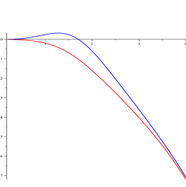
Figure 1: Comparison of the restricted and intrinsic Ricci forms on the space of centred hyperbolic two vortices: plots of $F|(s)$ (red) and $2F^{0}(s)$ (blue).

Magnetic geodesic flow on $M_{2}^{0}$ with respect to a rotationally invariant effective magnetic field ${\cal B}=F(s)ds\wedge\sigma_{2}$ is governed by the ODE system

$$\ddot{s} =-\frac{1}{2A_{1}(s)}\bigl{[}A_{1}^{\prime}(s)\dot{s}^{2}-A_{3}^{\prime}(s)\dot{\psi}^{2}+2F(s)\dot{\psi}\bigr{]},$$

$$\ddot{\psi} =-\frac{1}{A_{3}(s)}\bigl{[}A_{3}^{\prime}(s)\dot{s}\;\dot{\psi}-F(s)\dot{s}\bigr{]},$$ (3.60)

where $\psi$ is an angular coordinate chosen so that $d\psi=\sigma_{2}\rvert$. Choosing $F(s)$ to be $F\rvert(s)$ or $2F^{0}(s)$ we obtain the extrinsic and intrinsic RMG flows, respectively, normalized so as to coincide asymptotically at large $s$. We have solved these ODE systems numerically for various initial values. The corresponding RMG trajectories of one of the vortices on the Poincaré disk are depicted in Figure 2. As expected, RMG trajectories which reach the core region of $M_{2}^{0}$ exhibit marked differences in the two flows.

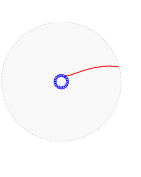
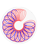
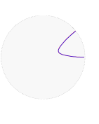
(a)	(b)	(c)

Figure 2: Plots of vortex trajectories under the extrinsic RMG flow on $M_{2}^{0}$ (red) and the intrinsic RMG flow (blue) with $\lambda_{\text{intrinsic}}=2\lambda_{\text{extrinsic}}$ and various initial values .

A related observation concerns orbiting vortex pairs. It is immediate from (3.60) that a circle of constant $s$ is a closed magnetic geodesic if and only if it is traversed at constant angular velocity

$$\dot{\psi}=\nu(s)=2\frac{F(s)}{A_{3}^{\prime}(s)}.$$ (3.61)

This, then, gives the frequency-separation relation for a pair of vortices orbiting one another at fixed separation. Note that $A_{3}^{\prime}(s)>0$ for all $s>0$. From figure 1, one sees that (for $\lambda>0$) vortex pairs obeying the intrinsic RMG flow orbit one another anticlockwise for $s<s_{0}\approx 1.7$ and clockwise for $s>s_{0}$, whereas orbiting vortex pairs always circulate clockwise in the extrinsic flow.

Unlike geodesics, the features of RMG flow on a fixed point set of a holomorphic isometry, such as $M_{2}^{0}$, cannot be deduced by knowing only the metric on the fixed point set. This difference makes RMG flow significantly harder to study than geodesic flow and means that studies of intrinsic RMG flow on low-dimensional submanifolds, such as those presented in [8], are of limited value in trying to understand the true (extrinsic) RMG flow.

4 RMG motion of $\mathbb{C}P^{1}$ lumps

As observed in section 1, the question of completeness of RMG flow on a noncompact kähler manifold is interesting and nontrivial. Certainly, if the manifold is complete (as a metric space or, equivalently, its geodesic flow is complete), then it is RMG complete since RMG flow conserves speed (so an RMG curve which escaped every compact set in bounded time would define a divergent Cauchy sequence). Since RMG flow converges (pointwise) to geodesic flow in the limit of large speed, it has been conjectured that the converse holds also: if a kähler manifold is RMG complete then it is geodesically complete [8]. In fact this is false, and in this section we provide a counterexample of independent interest: the moduli space of unit charge ${\mathbb{C}}{{P}}^{1}$ lumps on $S^{2}$, or, equivalently, the space ${\sf Rat}_{1}$ of degree one rational maps $S^{2}\rightarrow S^{2}$, given its $L^{2}$ metric.

Recall that ${\sf Rat}_{n}$ is the space of degree $n$ holomorphic maps $S^{2}\rightarrow S^{2}$. If one chooses stereographic coordinates $z,W$ on the domain and codomain, such maps take the form

$$W(z)=\frac{a_{0}+a_{1}z+\cdots+a_{n}z^{n}}{b_{0}+b_{1}z+\cdots+b_{n}z^{n}}$$ (4.1)

where $a_{0},\ldots,a_{n},b_{0},\ldots,b_{n}\in{\mathbb{C}}$ are constant. There is a natural inclusion ${\sf Rat}_{n}\hookrightarrow{\mathbb{C}}{{P}}^{2n+1}$ defined by $W(z)\mapsto[a_{0},\ldots,a_{n},b_{0},\ldots,b_{n}]$, which equips ${\sf Rat}_{n}$ with a complex structure, and a natural metric on ${\sf Rat}_{n}$ defined by restricting the $L^{2}$ norm on $W^{-1}TS^{2}$ to $T{\sf Rat}_{n}$. It is known [20] that ${\sf Rat}_{n}$ is kähler with respect to this metric and complex structure. Further, ${\sf Rat}_{1}$ is diffeomorphic to $SO(3)\times{\mathbb{R}}^{3}$. One may regard ${\cal O}\in SO(3)$ as parametrizing the internal orientation of the lump and $\mbox{\boldmath{$\lambda$}}\in{\mathbb{R}}^{3}$ as parametrizing both its sharpness, $\lambda=|\mbox{\boldmath{$\lambda$}}|$, and its position in physical space $-\mbox{\boldmath{$\lambda$}}/|\mbox{\boldmath{$\lambda$}}|\in S^{2}$. Lumps with $\mbox{\boldmath{$\lambda$}}=\mbox{\boldmath{$0$}}$ have sharpness $0$, that is, constant energy density, so do not have a well-defined position. Explicitly, the point $({\mathbb{I}}_{3},(0,0,\lambda))$ corresponds to the rational map

$$W(z)=\mu(\lambda)z,\qquad\mbox{where}\qquad\mu=\frac{\Lambda+\lambda}{\Lambda-\lambda}\qquad\mbox{and}\qquad\Lambda=\sqrt{1+\lambda^{2}},$$ (4.2)

and every other point in ${\sf Rat}_{1}$ can be reached from a point such as this by acting with some isometry: $G=SO(3)\times SO(3)$ acts isometrically on ${\sf Rat}_{1}$ via

$$({\cal L},{\cal R}):({\cal O},\mbox{\boldmath{$\lambda$}})\mapsto({\cal LOR}^{-1},{\cal R}\mbox{\boldmath{$\lambda$}}).$$ (4.3)

This is just the restiction to ${\sf Rat}_{1}$ of the natural action of $G$ on all smooth maps $S^{2}\rightarrow S^{2}$, namely, $({\cal L},{\cal R}):\phi\mapsto{\cal L}\circ\phi\circ{\cal R}^{-1}$.

$G$-invariance and the kähler property almost completely determine $\gamma_{L^{2}}$. By an argument similar to that used to prove Proposition 5, one finds [20] that

$$\gamma_{L^{2}}=A_{1}d\boldsymbol{\lambda}\cdot d\boldsymbol{\lambda}+A_{2}(\boldsymbol{\lambda}\cdot d\boldsymbol{\lambda})^{2}+A_{3}\boldsymbol{\sigma}\cdot\boldsymbol{\sigma}+A_{4}(\boldsymbol{\lambda}\cdot\boldsymbol{\sigma})^{2}+A_{5}\boldsymbol{\lambda}\cdot(\boldsymbol{\sigma}\times d\boldsymbol{\lambda}),$$ (4.4)

where $A_{1},\dots,A_{5}$ are smooth functions of $\lambda$ only defined by the single function

$$A(\lambda)=2\pi\mu\;\frac{[\mu^{4}-4\mu^{2}\log\mu-1]}{(\mu^{2}-1)^{3}},$$ (4.5)

as follows

$$A_{1} =A(\lambda),\qquad A_{2}=\frac{A(\lambda)}{\Lambda^{2}}+\frac{A^{\prime}(\lambda)}{\lambda},\qquad A_{3}=(\frac{1+2\lambda^{2}}{4})A(\lambda),$$

$$A_{4} =\biggl{(}\frac{\Lambda^{2}}{4\lambda}\biggr{)}A^{\prime}(\lambda),\qquad A_{5}=A(\lambda).$$ (4.6)

In (4.4) $\mbox{\boldmath{$\sigma$}}=(\sigma_{1},\sigma_{2},\sigma_{3})$ is the triple of left invariant one forms on $SO(3)$ dual to the left invariant vector fields $\theta_{1},\theta_{2},\theta_{3}$ which, at the identity ${\mathbb{I}}_{3}$, coincide with the usual basis for ${\mathfrak{so}}(3)$, that is

$$E_{1}=\left(\begin{array}[]{ccc}0&0&0\\ 0&0&-1\\ 0&1&0\end{array}\right),\qquad E_{2}=\left(\begin{array}[]{ccc}0&0&1\\ 0&0&0\\ -1&0&0\end{array}\right),\qquad E_{3}=\left(\begin{array}[]{ccc}0&-1&0\\ 1&0&0\\ 0&0&0\end{array}\right).$$ (4.7)

Also, $\times$ denotes vector product in ${\mathbb{R}}^{3}$, and juxtaposition of one-forms denotes symmetrized tensor product. Note that, although we are using similar notation to that of section 3.2, the functions $A_{i}$ and one-forms $\sigma_{i}$ in (4.4) are unrelated to the analogous quantities defined there. It follows immediately from (4.4) that ${\sf Rat}_{1}$ is geodesically incomplete (for example, the curve $({\mathbb{I}}_{3},(0,0,s))$ with $s\in{\mathbb{R}}$ has finite length).

Since ${\sf Rat}_{1}$ has trivial second cohomology, its Ricci form $\rho$ is necessarily exact. An explicit formula for $\rho$ was derived in [20], from which it quickly follows that

$$\rho=\mathrm{d}{\cal A},\qquad{\cal A}=\frac{\Lambda}{2}\bar{A}(\lambda)\>\;(\boldsymbol{\lambda}\cdot\boldsymbol{\sigma}),$$ (4.8)

where

$$\bar{A}(\lambda)=-\frac{1}{2\lambda}\frac{d}{d\lambda}\log(A^{2}(\lambda)\;B(\lambda)),$$ (4.9)

and

$$B(\lambda):=A_{3}(\lambda)+\lambda^{2}A_{4}(\lambda)=\frac{1+2\lambda^{2}}{4}A(\lambda)+\frac{\lambda\Lambda^{2}}{4}A^{\prime}(\lambda)=\frac{\Lambda}{4}\frac{d}{d\lambda}(\lambda\Lambda A(\lambda)).$$ (4.10)

Hence RMG flow on ${\sf Rat}_{1}$ is governed by the Lagrangian

$$L=\frac{1}{2}[A_{1}(\dot{\boldsymbol{\lambda}}\cdot\dot{\boldsymbol{\lambda}})+A_{2}(\boldsymbol{\lambda}\cdot\dot{\boldsymbol{\lambda}})^{2}+A_{3}(\boldsymbol{\Omega}\cdot\boldsymbol{\Omega})+A_{4}(\boldsymbol{\lambda}\cdot\boldsymbol{\Omega})^{2}+A_{5}\boldsymbol{\lambda}\cdot(\boldsymbol{\Omega}\times\dot{\boldsymbol{\lambda}})-\Lambda\bar{A}(\boldsymbol{\lambda}\cdot\boldsymbol{\Omega})]$$ (4.11)

for a curve $\chi(t)=({\cal O}(t),\boldsymbol{\lambda}(t))$ on ${\sf Rat}_{1}$ whose angular velocity $\mbox{\boldmath{$\Omega$}}\in{\mathbb{R}}^{3}$ is defined such that ${\cal O}(t)^{-1}\dot{\cal O}(t)=\mbox{\boldmath{$\Omega$}}\cdot\mbox{\boldmath{$E$}}\in{\mathfrak{so}}(3)$. Note that, to avoid confusion with the radial coordinate $\lambda=\|\mbox{\boldmath{$\lambda$}}\|$, we have used the scaling property of RMG flow to set the effective electric charge (denoted $\lambda$ in section 1) to unity. This flow conserves total energy

$$E=\frac{1}{2}[A_{1}(\dot{\boldsymbol{\lambda}}\cdot\dot{\boldsymbol{\lambda}})+A_{2}(\boldsymbol{\lambda}\cdot\dot{\boldsymbol{\lambda}})^{2}+A_{3}(\boldsymbol{\Omega}\cdot\boldsymbol{\Omega})+A_{4}(\boldsymbol{\lambda}\cdot\boldsymbol{\Omega})^{2}+A_{5}\boldsymbol{\lambda}\cdot(\boldsymbol{\Omega}\times\dot{\boldsymbol{\lambda}})].$$ (4.12)

Furthermore, we have

Proposition 9

RMG flow on ${\sf Rat}_{1}$ conserves the angular momenta $\{P_{k},Q_{k}:k=1,2,3\}$ given by

$$P_{k} =\sum_{j=1,2,3}{\cal O}_{jk}[A_{3}\Omega_{j}+A_{4}(\boldsymbol{\Omega}\cdot\boldsymbol{\lambda})\lambda_{j}+\frac{1}{2}A_{1}(\dot{\boldsymbol{\lambda}}\times\boldsymbol{\lambda}))_{j}-\frac{1}{2}\Lambda\bar{A}\lambda_{j}],$$ (4.13)

$$Q_{k} =(A_{3}-\frac{1}{2}\lambda^{2}A_{1})\Omega_{k}+(A_{4}+\frac{1}{2}A_{1})(\boldsymbol{\Omega}\cdot\boldsymbol{\lambda})\lambda_{k}-\frac{1}{2}A_{1}(\dot{\boldsymbol{\lambda}}\times\boldsymbol{\lambda})_{k}-\frac{1}{2}\Lambda\bar{A}\lambda_{k}.$$ (4.14)

Proof.

The RMG Lagrangian, given in (4.11), has $G=SO(3)\times SO(3)$ symmetry. Hence, there is a set of six conserved angular momenta, one for each generator of $G$. Given $\bar{Y}\in\mathfrak{g}={\mathfrak{so}}(3)\oplus{\mathfrak{so}}(3)$, denote by $Y$ the killing vector field on ${\sf Rat}_{1}$ which it induces. Then the conserved Noether charge associated with the infinitesimal symmetry $\bar{Y}$ is [14]

$$\text{J}_{Y}=\gamma_{L^{2}}(Y,\dot{\chi})-{\cal A}(Y)+\alpha_{Y},$$ (4.15)

where $\alpha_{Y}$ is a real function on ${\sf Rat}_{1}$ such that $\mathrm{d}\alpha_{Y}=\mathcal{L}_{Y}{\cal A}$. Since ${\cal A}$ is $G$-invariant, $\mathcal{L}_{Y}{\cal A}=0$ for all $\bar{Y}$, so we may take $\alpha_{Y}=0$ for all $\bar{Y}$.

The six killing vector fields on ${\sf Rat}_{1}=SO(3)\times{\mathbb{R}}^{3}$ generated by the usual basis for $\mathfrak{g}$ are [9]

$$\xi_{k},\qquad Z_{k}=\theta_{k}+\sum_{i,j}\epsilon_{kij}\lambda_{i}\frac{\partial\>}{\partial\lambda_{j}},\qquad k=1,2,3$$ (4.16)

where $\theta_{i}$ are, as before, the left invariant vector fields on $SO(3)$ dual to $\sigma_{i}$, and $\xi_{i}$ are the right invariant vector fields on $SO(3)$ with $\xi_{i}({\mathbb{I}}_{3})=\theta_{i}({\mathbb{I}}_{3})$, explicitly,

$$\xi_{k}=\sum_{j}{\cal O}_{jk}\;\theta_{j}.$$ (4.17)

Setting $Y=\xi_{k}$ in (4.15) yields the conserved charge $\text{J}_{Y}=P_{k}$ claimed, and similarly setting $Y=Z_{k}$ yields the charge $Q_{k}$. ∎

It is convenient to collect the angular momenta $\{P_{k}:k=1,2,3\}$ and $\{Q_{k}:k=1,2,3\}$ into a pair of 3-vectors

$$\boldsymbol{P} ={\cal O}^{T}[A_{3}\boldsymbol{\Omega}+A_{4}(\boldsymbol{\Omega}\cdot\boldsymbol{\lambda})\boldsymbol{\lambda}+\frac{1}{2}A_{1}(\dot{\boldsymbol{\lambda}}\times\boldsymbol{\lambda}))-\frac{1}{2}\Lambda\bar{A}\boldsymbol{\lambda}],$$ (4.18)

$$\boldsymbol{Q} =(A_{3}-\frac{1}{2}\lambda^{2}A_{1})\boldsymbol{\Omega}+(A_{4}+\frac{1}{2}A_{1})(\boldsymbol{\Omega}\cdot\boldsymbol{\lambda})\boldsymbol{\lambda}-\frac{1}{2}A_{1}(\dot{\boldsymbol{\lambda}}\times\boldsymbol{\lambda})-\frac{1}{2}\Lambda\bar{A}\boldsymbol{\lambda}.$$ (4.19)

Having determined the conserved quantities $E$, $\boldsymbol{P}$ and $\boldsymbol{Q}$ associated with the RMG flow on ${\sf Rat}_{1}$, one can eliminate $\boldsymbol{\Omega}$ from $E$ to obtain

$$E= \frac{1}{2}\biggl{(}A_{1}\|\dot{\boldsymbol{\lambda}}\|^{2}+A_{2}(\boldsymbol{\lambda}\cdot\dot{\boldsymbol{\lambda}})^{2}+\frac{1}{A_{3}}\|\boldsymbol{P}\|^{2}-\frac{A_{1}^{2}}{4A_{3}}\|\dot{\boldsymbol{\lambda}}\times\boldsymbol{\lambda}\|^{2}+\frac{\Lambda\bar{A}}{A_{3}}(\boldsymbol{Q}\cdot\boldsymbol{\lambda})$$

$$-\frac{A_{4}}{A_{3}B}\;[(\boldsymbol{Q}\cdot\boldsymbol{\lambda})+\frac{1}{2}\lambda^{2}\Lambda\bar{A}]^{2}+\frac{\lambda^{2}\Lambda^{2}\bar{A}^{2}}{4A_{3}}\biggr{)}.$$ (4.20)

Consider the mapping $q:T{\sf Rat}_{1}\rightarrow{\mathbb{R}}\times{\mathbb{R}}^{3}\times{\mathbb{R}}^{3}$ which assigns to each tangent vector the triple $(E,\boldsymbol{P},\boldsymbol{Q})$. By Proposition 9, every RMG curve in ${\sf Rat}_{1}$ is confined to some level set of $q$. That RMG flow is complete will follow quickly from the following:

Theorem 10

Every level set of $q:T{\sf Rat}_{1}\rightarrow{\mathbb{R}}\times{\mathbb{R}}^{3}\times{\mathbb{R}}^{3}$ is compact.

Proof.

Choose and fix $(E,\boldsymbol{P},\boldsymbol{Q})\in{\mathbb{R}}^{7}$ and let $X=q^{-1}(E,\boldsymbol{P},\boldsymbol{Q})\subset T{\sf Rat}_{1}$. Now $T{\sf Rat}_{1}\equiv TSO(3)\times T{\mathbb{R}}^{3}$, and $TSO(3)\equiv SO(3)\times{\mathbb{R}}^{3}$ via the identification $\dot{\cal O}\mapsto\mbox{\boldmath{$\Omega$}}$. We may realize $SO(3)$ as a submanifold of ${\mathbb{R}}^{9}$ by mapping ${\cal O}$ to its list of matrix elements. In this way, we may regard $T{\sf Rat}_{1}$ as a 12-dimensional submanifold of ${\mathbb{R}}^{9}\times{\mathbb{R}}^{3}\times{\mathbb{R}}^{3}\times{\mathbb{R}}^{3}$. The mapping $q$ is smooth, hence certainly continuous, so $X$ is closed. Hence, by Heine-Borel, it suffices to show that $X\subset{\mathbb{R}}^{18}$ is bounded in euclidean norm.

Assume, towards a contradiction, that there is some sequence $x_{n}=({\cal O}_{n},\mbox{\boldmath{$\Omega$}}_{n},\mbox{\boldmath{$\lambda$}}_{n},\dot{}\mbox{\boldmath{$\lambda$}}_{n})\in X$ which is unbounded in euclidean norm. By the definition of $SO(3)$, $\|{\cal O}_{n}\|_{{\mathbb{R}}^{9}}=\sqrt{3}$ for all $n$, so (at least) one of $\mbox{\boldmath{$\lambda$}}_{n},\dot{}\mbox{\boldmath{$\lambda$}}_{n},\mbox{\boldmath{$\Omega$}}_{n}$ must be unbounded. We will now eliminate these possibilities in turn.

Assume $\mbox{\boldmath{$\lambda$}}_{n}$ is unbounded. Then it has a subsequence, which we still denote $\mbox{\boldmath{$\lambda$}}_{n}$, with $\|\mbox{\boldmath{$\lambda$}}_{n}\|\rightarrow\infty$. For all $\mbox{\boldmath{$\lambda$}}\neq\mbox{\boldmath{$0$}}$ let $\hat{}\mbox{\boldmath{$\lambda$}}=\mbox{\boldmath{$\lambda$}}/\|\mbox{\boldmath{$\lambda$}}\|$ and

$$H(\boldsymbol{\lambda},\dot{\boldsymbol{\lambda}}) :=A_{1}\|\dot{\boldsymbol{\lambda}}\|^{2}+\lambda^{2}A_{2}(\hat{\boldsymbol{\lambda}}\cdot\dot{\boldsymbol{\lambda}})^{2}-\frac{\lambda^{2}A_{1}^{2}}{4A_{3}}\|\hat{\boldsymbol{\lambda}}\times\dot{\boldsymbol{\lambda}}\|^{2},$$ (4.21)

$$G(\boldsymbol{\lambda},\boldsymbol{Q}) :=F_{1}(\lambda)\;(\boldsymbol{Q}\cdot\hat{\boldsymbol{\lambda}})^{2}\;+F_{2}(\lambda)\;(\boldsymbol{Q}\cdot\hat{\boldsymbol{\lambda}})\;+F_{3}(\lambda),$$ (4.22)

where

$$F_{1}(\lambda)=-\frac{\lambda^{2}A_{4}}{A_{3}B},\qquad F_{2}(\lambda)=\frac{\lambda\Lambda\bar{A}}{A_{3}}\biggl{(}1-\frac{\lambda^{2}A_{4}}{B}\biggr{)},\qquad F_{3}(\lambda)=\frac{\lambda^{2}\Lambda^{2}\bar{A}^{2}}{4B}.$$ (4.23)

Then, the conserved energy $E$, given in (4.20), can be written as

$$E=\frac{1}{2}\biggl{(}H(\boldsymbol{\lambda},\dot{\boldsymbol{\lambda}})+\frac{1}{A_{3}}\|\boldsymbol{P}\|^{2}+G(\boldsymbol{\lambda},\boldsymbol{Q})\biggr{)}.$$ (4.24)

Since the cross and dot products on $\mathbb{R}^{3}$ are related by

$$\|\hat{\boldsymbol{\lambda}}\times\dot{\boldsymbol{\lambda}}\|^{2}=\|\dot{\boldsymbol{\lambda}}\|^{2}-(\hat{\boldsymbol{\lambda}}\cdot\dot{\boldsymbol{\lambda}})^{2},$$ (4.25)

then,

$$H(\boldsymbol{\lambda},\dot{\boldsymbol{\lambda}}) =\frac{\Lambda^{2}A}{1+2\lambda^{2}}\;\|\dot{\boldsymbol{\lambda}}\|^{2}+\lambda^{2}\biggl{(}\frac{2+3\lambda^{2}}{(1+2\lambda^{2})\Lambda^{2}}A+\frac{A^{\prime}(\lambda)}{\lambda}\biggr{)}(\hat{\boldsymbol{\lambda}}\cdot\dot{\boldsymbol{\lambda}})^{2}.$$ (4.26)

Here, we have used the definition of $A_{1},A_{2}$ and $A_{3}$, as in (4.6). Since $B(\lambda)$, given in (4.10), is positive,

$$\frac{A^{\prime}(\lambda)}{\lambda}>-\frac{1+2\lambda^{2}}{\lambda^{2}\Lambda^{2}}A,$$ (4.27)

from which it follows that

$$H(\boldsymbol{\lambda},\dot{\boldsymbol{\lambda}})\geq\frac{\Lambda^{2}A}{1+2\lambda^{2}}\;\|\hat{\boldsymbol{\lambda}}\times\dot{\boldsymbol{\lambda}}\|^{2}\geq 0.$$ (4.28)

Since both $H(\boldsymbol{\lambda},\dot{\boldsymbol{\lambda}})$ and $A_{3}$ are non-negative, it follows from (4.24) that

$$2E\geq G(\boldsymbol{\lambda}_{n},\boldsymbol{Q}).$$ (4.29)

From (4.5), one obtains the following limit

$$\lim_{\lambda\rightarrow\infty}\;\frac{\log\lambda}{\lambda^{4}}\;G(\boldsymbol{\lambda},\boldsymbol{Q})=\frac{4}{\pi}[(\boldsymbol{Q}\cdot\hat{\boldsymbol{\lambda}})+2]^{2}.$$ (4.30)

But $\|\mbox{\boldmath{$\lambda$}}_{n}\|\rightarrow\infty$, so (4.30) contradicts (4.29) unless $\|\boldsymbol{Q}\|=2$.

Hence $\|\boldsymbol{Q}\|=2$. Let $\theta$ be the angle between $\boldsymbol{\lambda}$ and $\boldsymbol{Q}$, namely,

$$\boldsymbol{Q}\cdot\hat{\boldsymbol{\lambda}}=\|\boldsymbol{Q}\|\cos\theta=2\cos\theta.$$ (4.31)

Then, it follows from (4.22) that

$$G(\boldsymbol{\lambda},\boldsymbol{Q})=4F_{1}(\lambda)\cos^{2}\theta+2F_{2}(\lambda)\cos\theta+F_{3}(\lambda)=:Z(\lambda,\theta).$$ (4.32)

We shall appeal to the following technical lemma whose proof we postpone to an appendix.

Lemma 11

On $({\sf Rat}_{1},\gamma_{L^{2}})$, there exist $c_{0},\lambda_{0}>0$ such that for all $\lambda\geq\lambda_{0}$, $Z(\lambda,\theta)$, given in (4.32), satisfies

$$Z(\lambda,\theta)>\frac{c_{0}\lambda^{4}}{(\log\lambda)^{3}},\quad\forall\>\theta\in\mathbb{R}.$$ (4.33)

Using the above lemma, it follows from (4.29), (4.32) and (4.33) that, for all $n$ sufficiently large,

$$2E\geq G(\boldsymbol{\lambda}_{n},\boldsymbol{Q})>\frac{c_{0}\|\mbox{\boldmath{$\lambda$}}_{n}\|^{4}}{(\log\|\mbox{\boldmath{$\lambda$}}_{n}\|)^{3}},$$ (4.34)

a contradiction. Hence $\mbox{\boldmath{$\lambda$}}_{n}$ is bounded.

Assume now that $\dot{}\mbox{\boldmath{$\lambda$}}_{n}$ is unbounded. We have shown that $\|\mbox{\boldmath{$\lambda$}}_{n}\|$ is confined to a closed bounded interval, so $A_{i}(\|\mbox{\boldmath{$\lambda$}}_{n}\|)$, $B(\|\mbox{\boldmath{$\lambda$}}_{n}\|)$ are positive, bounded and bounded away from zero, and $\overline{A}(\|\mbox{\boldmath{$\lambda$}}_{n}\|)$ is bounded, by continuity. Hence, from (4.20) we see that

$$2E>A_{1}(\|\mbox{\boldmath{$\lambda$}}_{n}\|)\left(1-\frac{\|\mbox{\boldmath{$\lambda$}}_{n}\|^{2}A_{1}(\|\mbox{\boldmath{$\lambda$}}_{n}\|)}{4A_{3}(\|\mbox{\boldmath{$\lambda$}}_{n}\|)}\right)\|\dot{}\mbox{\boldmath{$\lambda$}}_{n}\|^{2}+c=A_{1}(\|\mbox{\boldmath{$\lambda$}}_{n}\|)\frac{2\|\mbox{\boldmath{$\lambda$}}_{n}\|^{2}}{1+2\|\mbox{\boldmath{$\lambda$}}_{n}\|^{2}}\|\dot{}\mbox{\boldmath{$\lambda$}}_{n}\|^{2}+c$$ (4.35)

for some constant $c\in{\mathbb{R}}$. But this contradicts unboundedness of $\dot{}\mbox{\boldmath{$\lambda$}}_{n}$.

Finally, assume that $\|\mbox{\boldmath{$\Omega$}}_{n}\|$ is unbounded. We have already shown that $\|\mbox{\boldmath{$\lambda$}}_{n}\|$ and $\|\dot{}\mbox{\boldmath{$\lambda$}}_{n}\|$ are bounded, and by continuity, $A_{i}(\|\mbox{\boldmath{$\lambda$}}_{n}\|)$ are positive, bounded and bounded away from $0$. But this immediately contradicts (4.12). ∎

Corollary 12

$({\sf Rat}_{1},\gamma_{L^{2}})$ is RMG complete.

Proof.

For each $K>0$, let $X_{K}=\{({\cal O},\mbox{\boldmath{$\Omega$}},\mbox{\boldmath{$\lambda$}},\dot{}\mbox{\boldmath{$\lambda$}}\in T{\sf Rat}_{1}\>:\>\|\mbox{\boldmath{$\Omega$}}\|+\|\mbox{\boldmath{$\lambda$}}\|+\|\dot{}\mbox{\boldmath{$\lambda$}}\|)\leq K\}$. By a standard application of Picard’s method, there exists $T_{K}>0$, depending only on $K$, such that, for all $x_{0}\in X_{K}$ there exists a unique RMG curve $x:[-T_{K},T_{K}]\rightarrow X_{2K}$ with $x(0)=x_{0}$. Now choose and fix $x_{0}\in T{\sf Rat}_{1}$, and let $X=q^{-1}(q(x_{0}))$, the level set of $q$ containing $x_{0}$. By Theorem 10, there exists $K>0$ such that $X\subset X_{K}$. Hence there is a unique RMG curve $x:[-T_{K},T_{K}]\rightarrow X_{2K}$ with $x(0)=x_{0}$. But, by Proposition 9, $x(\pm T_{K})\in X\subset X_{K}$, so this solution can be extended, both forward and backward in time, to $[-3T_{K},3T_{K}]$, and $x(\pm 3T_{K})\in X\subset X_{K}$ also. Proceeding inductively, the RMG curve has an extension $x:{\mathbb{R}}\rightarrow X_{K}$. Since $x_{0}$ was arbitrary, it follows that RMG flow is complete. ∎

Remark 13

Theorem 10 is strictly stronger than Corollary 12, since it implies that every RMG curve in $({\sf Rat}_{1},\gamma_{L^{2}})$ is confined to a compact subset of ${\sf Rat}_{1}$ and hence is bounded away from the boundary of ${\sf Rat}_{1}$ at infinity. This is not true of complete RMG flows in general (consider for example the trivial RMG flow on ${\mathbb{C}}^{n}$).

Remark 14

Since $({\sf Rat}_{1},\gamma_{L^{2}})$ is known to be geodesically incomplete, it is a counterexample to the conjecture [8] that every RMG complete kähler manifold is geodesically complete. Simpler counterexamples can be constructed. For example the surface of revolution ${\mathbb{C}}$ given the metric $g={\rm sech}\,|z|\>dzd\bar{z}$ is manifestly geodesically incomplete and can be shown, by an energy/angular momentum conservation argument analogous to the one presented here for ${\sf Rat}_{1}$, to be RMG complete [1].

The $L^{2}$ geometry of ${\sf Rat}_{n}$, for $n\geq 2$, is comparatively poorly understood. It is known to be $G$-invariant, kähler and geodesically incomplete [20], and is conjectured to have finite total volume [3]. Inside ${\sf Rat}_{n}$ there is a topologically cylindrical submanifold, ${\sf Rat}_{n}^{eq}$, the fixed point set of the circle group of isometries $W(z)\mapsto e^{in\alpha}W(e^{-i\alpha}z)$. This consists of rotationally equivariant rational maps, of the form $W(z)=cz^{n}$, where $c\in{\mathbb{C}}^{\times}={\mathbb{C}}\backslash\{0\}$, and is preserved by (extrinsic) RMG flow on ${\sf Rat}_{n}$ by Corollary 2. The induced $L^{2}$ metric on ${\sf Rat}_{n}^{eq}$ was studied in detail in [15]. It is interesting to compare the intrinsic RMG flow on ${\sf Rat}_{n}^{eq}$ with the extrinsic RMG flow, defined by its inclusion in ${\sf Rat}_{n}$.

Denote by $\pi:{\mathbb{C}}^{\times}\rightarrow{\sf Rat}_{n}^{eq}$ the $n$-fold covering map $a\mapsto[W:z\mapsto(az)^{n}]$. Then the lifted $L^{2}$ metric on ${\mathbb{C}}^{\times}$ is

$$\pi^{*}\gamma_{L^{2}}^{eq}=F(|a|)dad\bar{a},\qquad F(\rho)=\pi n^{2}\int_{0}^{\infty}\frac{s^{n}}{(1+s^{n})^{2}}\frac{ds}{(\rho^{2}+s)^{2}}.$$ (4.36)

Now $c\mapsto c^{-1}$ is an isometry of ${\sf Rat}_{n}^{eq}$, whence it follows that $a\mapsto a^{-1}$ is an isometry of the lifted metric. Furthermore, $\lim_{\rho\rightarrow\infty}F(\rho)$ exists for all $n\geq 2$, so $\pi^{*}\gamma_{L^{2}}^{eq}$ has a $C^{0}$ extension to $S^{2}={\mathbb{C}}^{\times}\cup\{0,\infty\}$ for all $n\geq 2$, which we denote $\overline{\gamma}_{n}$. For $n$ sufficiently large, we can obtain useful information about RMG flow on $({\sf Rat}_{n}^{eq},\gamma_{L^{2}}^{eq})$ by considering its lift to $(S^{2},\overline{\gamma}_{n})$. This requires us to establish enhanced regularity of $\overline{\gamma}_{n}$, as follows.

Proposition 15

For all $n\geq 5$, the extended lifted metric $\overline{\gamma}_{n}$ on $S^{2}$ is $C^{3}$.

Proof.

It is known [15] that $\overline{\gamma}_{n}$ is $C^{2}$ for all $n\geq 4$. Further, $\overline{\gamma}_{n}$ is manifestly smooth on $S^{2}\backslash\{0,\infty\}$ so, in light of the isometry $a\mapsto 1/a$, which interchanges $0$ and $\infty$, it suffices to prove that $f_{xxx},f_{xxy},f_{xyy}$ and $f_{yyy}$ exist at $(0,0)$, where $f(x,y)=F(\sqrt{x^{2}+y^{2}})$. By computing in polar coordinates, $(x,y)=\rho(\cos\theta,\sin\theta)$, one sees that all these third derivatives exist (and vanish) if and only if

$$\lim_{\rho\rightarrow 0}\frac{1}{\rho}\left(F^{\prime\prime}(\rho)-\frac{F^{\prime}(\rho)}{\rho}\right) = 0$$

$$\lim_{\rho\rightarrow 0}\left(F^{\prime\prime\prime}(\rho)-\frac{3}{\rho}\left(F^{\prime\prime}(\rho)-\frac{F^{\prime}(\rho)}{\rho}\right)\right) = 0.$$ (4.37)

For each pair of integers $n\geq 2$ and $k\geq 0$, define the function $\eta_{n,k}:(0,\infty)\rightarrow{\mathbb{R}}$,

$$\eta_{n,k}(\rho)=\int_{0}^{\infty}\frac{s^{n}}{(1+s^{n})^{2}}\frac{ds}{(\rho^{2}+s)^{k}}.$$ (4.38)

For $0\leq k\leq n$, its integrand is bounded above by the integrable function $s^{n-k}/(1+s^{n})^{2}$, so, by the Lebesgue Dominated Convergence Theorem,

$$\lim_{\rho\rightarrow 0}\eta_{n,k}(\rho)=\int_{0}^{\infty}\frac{s^{n-k}}{(1+s^{n})^{2}}ds<\infty.$$ (4.39)

It follows from the definition of $F$ that

$$\frac{1}{\rho}\left(F^{\prime\prime}(\rho)-\frac{F^{\prime}(\rho)}{\rho}\right) = 24\pi n^{2}\rho\eta_{n,4}(\rho)$$ (4.40)

$$F^{\prime\prime\prime}(\rho)-\frac{3}{\rho}\left(F^{\prime\prime}(\rho)-\frac{F^{\prime}(\rho)}{\rho}\right) = -129\pi n^{2}\rho^{3}\eta_{n,5}(\rho).$$ (4.41)

Hence the required limits (4.37) follow from (4.39) provided $n\geq 5$. ∎

Corollary 16

For all $n\geq 5$, the intrinsic RMG flow on $({\sf Rat}_{n}^{eq},\gamma_{L^{2}}^{eq})$ is incomplete.

Proof.

Assume $n\geq 5$. Then $\overline{\gamma}_{n}$ is $C^{3}$, so its Ricci form is $C^{1}$. Hence, by standard existence and uniqueness theory of ODEs, the RMG flow is globally well-defined on $(S^{2},\overline{\gamma}_{n})$. In particular, there is an RMG curve $a:(-\varepsilon,\varepsilon)\rightarrow S^{2}$ with $a(0)=0$ and $\dot{a}(0)=1$. Consider the image of $a:(-\varepsilon,0)\rightarrow S^{2}$ under the projection $\pi:{\mathbb{C}}^{\times}\rightarrow{\sf Rat}_{n}^{eq}$. By definition, $\pi$ is a holomorphic isometry, so $\pi\circ a$ is an RMG curve in ${\sf Rat}_{n}^{eq}$, which reaches the singular point $a=0$ in finite time. Hence intrinsic RMG flow in ${\sf Rat}_{n}^{eq}$ is incomplete. ∎

Remark 17

By resorting to a case-by-case analysis of the flow on ${\sf Rat}_{n}^{eq}$ itself, one can extend the conclusion of Corollary 16 to all $n\geq 2$ [1]. The case $n=2$ is considered below, see Proposition 19.

As we have remarked, the extrinsic RMG flow on a totally geodesic complex submanifold of a kähler manifold does not, in general, coincide with its intrinsic RMG flow, so we cannot conclude from Corollary 16 that $({\sf Rat}_{n},\gamma_{L^{2}})$ is RMG incomplete for $n\geq 5$: this would follow if the extrinsic RMG flow on ${\sf Rat}_{n}^{eq}$ were incomplete. Remarkably, although we have little information about the $L^{2}$ metric on ${\sf Rat}_{2}$, we have enough to prove that the extrinsic RMG flow on ${\sf Rat}_{2}^{eq}$ is complete. This follows from the following formula for the restriction of the Ricci form to ${\sf Rat}_{n}^{eq}$.

Proposition 18

Let $\rho\rvert$ be the restriction of the Ricci form $\rho$ of $({\sf Rat}_{n},\gamma_{L^{2}})$ to ${\sf Rat}_{n}^{eq}$ (that is, $\rho\rvert=\iota^{*}\rho$ where $\iota:{\sf Rat}_{n}^{eq}\rightarrow{\sf Rat}_{n}$ denotes inclusion) and $\rho^{eq}$ be the intrinsic Ricci form on $({\sf Rat}_{n}^{eq},\gamma_{L^{2}}^{eq})$. Then $\rho\rvert=\mathrm{d}{\cal A}\rvert$ and $\rho^{eq}=\mathrm{d}{\cal A}^{eq}$ where

$${\cal A}\rvert = -\left(\sum_{j=0}^{2n}\frac{|\chi|F_{j}^{\prime}(\chi)}{2F_{j}(\chi)}\right)d\psi,$$

$${\cal A}^{eq} = -\frac{\chi F_{n}^{\prime}(\chi)}{2F_{n}(\chi)}\>d\psi,$$

and

$$F_{j}(\chi)=16\pi\int_{0}^{\infty}\frac{s^{j}}{(1+\chi^{2}s^{n})^{2}}\frac{ds}{(1+s)^{2}}.$$

The coordinate $\chi e^{i\psi}$ on ${\sf Rat}_{n}^{eq}\equiv{\mathbb{C}}^{\times}$ corresponds to the rational map $W(z)=\chi e^{i\psi}z^{n}$.

Proof.

${\sf Rat}_{n}^{eq}$ lies entirely within the coordinate chart on ${\sf Rat}_{n}$ on which

$$W(z)=\frac{a_{0}+a_{1}z+\cdots+a_{n}z^{n}}{1+a_{n+1}z+\cdots+a_{2n}z^{n}}.$$ (4.42)

It is the surface $a_{0}=\cdots=a_{n-1}=a_{n+1}=\cdots=a_{2n}=0$, $a_{n}=\chi e^{i\psi}\in{\mathbb{C}}^{\times}$. Let $G(a_{0},\ldots,a_{2n})=\log\det\gamma_{\cdot\bar{\cdot}}$ where $\gamma_{\cdot\bar{\cdot}}$ denotes the hermitian matrix of metric coefficients of $\gamma$ with respect to the local complex coordinates $a_{j}$. Then [5, p. 82],

$$\rho=-i\partial\bar{\partial}G,$$ (4.43)

so

$$\rho\rvert=-i\iota^{*}\partial\bar{\partial}G=-i\partial\bar{\partial}(G\circ\iota)$$ (4.44)

since the inclusion is holomorphic. Now

$$\gamma_{j\bar{k}}=16\int_{\mathbb{C}}\frac{1}{(1+|W(z)|^{2})^{2}}\frac{\partial W}{\partial a_{j}}\overline{\left(\frac{\partial W}{\partial a_{k}}\right)}\frac{dzd\bar{z}}{(1+|z|^{2})^{2}}$$ (4.45)

and

$$\left.\frac{\partial W}{\partial a_{j}}\right|=\left\{\begin{array}[]{cc}z^{j}&0\leq j\leq n\\ -\chi e^{i\psi}z^{j}&n+1\leq j\leq 2n\end{array}\right.$$ (4.46)

where the vertical stroke denotes evaluation at the rational map $\chi e^{i\psi}z^{n}$. It follows that $\gamma_{j\bar{k}}\rvert=0$ if $j\neq k$, and that

$$\gamma_{j\bar{j}}\rvert=\left\{\begin{array}[]{cc}F_{j}(\chi)&0\leq j\leq n\\ \chi^{2}F_{j}(\chi)&n+1\leq j\leq 2n.\end{array}\right.$$ (4.47)

Hence

$$G\circ\iota=n\log\chi^{2}+\sum_{j=0}^{2n}\log F_{j}(\chi),$$ (4.48)

and the formula for $\rho\rvert$ immediately follows. To obtain the formula for $\rho^{eq}$ we note that the induced metric on ${\sf Rat}_{n}^{eq}$ is

$$\gamma_{L^{2}}^{eq}=\gamma_{n\bar{n}}\rvert da_{n}d\bar{a}_{n}=F_{n}(\chi)dcd\bar{c},$$ (4.49)

where $c=\chi e^{i\psi}$, and use (4.43). ∎

Since the integrand in $F_{j}$ is rational, one can, in principle, evaluate each of these functions as an explicit function of $\chi$. The expressions involved become very complicated as $n$ grows large, however.

Both extrinsic and intrinsic RMG flow on ${\sf Rat}_{n}^{eq}$ are governed by a lagrangian of the form

$$L=\frac{1}{2}F_{n}(\chi)(\dot{\chi}^{2}+\chi^{2}\dot{\psi}^{2})-a(\chi)\dot{\psi}$$ (4.50)

where $a(\chi)={\cal A}^{eq}(\partial/\partial\psi)$ or $a(\chi)={\cal A}\rvert(\partial/\partial\psi)$ respectively. In each case, both the momentum conjugate to $\psi$,

$$P=\chi^{2}F_{n}(\chi)\dot{\psi}-a(\chi)$$ (4.51)

and the kinetic energy

$$E=\frac{1}{2}F_{n}(\chi)(\dot{\chi}^{2}+\chi^{2}\dot{\psi}^{2})=\frac{1}{2}F_{n}(\chi)\dot{\chi}^{2}+\frac{(P+a(\chi))^{2}}{2\chi^{2}F_{n}(\chi)}$$ (4.52)

are conserved. This is equivalent to motion on $(0,\infty)$ with the metric $F_{n}(\chi)d\chi^{2}$ in the effective potential

$$V_{P}(\chi)=\frac{(P+a(\chi))^{2}}{2\chi^{2}F_{n}(\chi)}.$$ (4.53)

Since $(0,\infty)$ has finite total length with respect to this metric [17], the flow is complete if and only if, for each $P\in{\mathbb{R}}$, the effective potential is unbounded above as $\chi\rightarrow 0$ and $\chi\rightarrow\infty$. Both the intrinsic and extrinsic RMG flows are symmetric under $c=\chi e^{i\psi}\mapsto 1/c$, so in fact it suffices to consider $V_{P}(\chi)$ in a neighbourhood of $0$.

Proposition 19

${\sf Rat}_{2}^{eq}$ is extrinsically RMG complete with respect to the $L^{2}$ metric, but intrinsically RMG incomplete.

Proof.

As argued above, we must show that the effective potential $V_{P}$ is unbounded above as $\chi\rightarrow 0$ for all $P$, in the case of extrinsic flow, and is bounded as $\chi\rightarrow 0$ for at least one choice of $P$ in the case of intrinsic flow. Let $G_{j}(\chi)=-\frac{1}{2}\chi F_{j}^{\prime}(\chi)/F_{j}(\chi)$, and $G(\chi)=\sum_{j=0}^{4}G_{j}(\chi)$. Then the effective potentials governing the extrinsic and intrinsic RMG flows are

$$V_{P}^{ext}(\chi)=\frac{(P+G(\chi))^{2}}{2\chi^{2}F_{2}(\chi)},\qquad V_{P}^{int}(\chi)=\frac{(P+G_{2}(\chi))^{2}}{2\chi^{2}F_{2}(\chi)},\qquad$$ (4.54)

respectively. With the aid of Maple, for example, one can obtain the following limits:

$$\lim_{\chi\rightarrow 0}\chi F_{2}(\chi)=4\pi,\qquad\lim_{\chi\rightarrow 0}\frac{G_{2}(\chi)-\frac{1}{2}}{\chi\log\chi}=-\frac{4}{\pi},\qquad\lim_{\chi\rightarrow 0}(G(\chi)-3)\log\chi=-\frac{1}{2}.$$ (4.55)

It follows that, for all $P\neq-3$,

$$\lim_{\chi\rightarrow 0}\chi V^{ext}_{P}(\chi)=\frac{(P+3)^{2}}{8\pi}$$ (4.56)

and

$$\lim_{\chi\rightarrow 0}\chi(\log\chi)^{2}V^{ext}_{-3}(\chi)=\frac{1}{32\pi}.$$ (4.57)

Hence, for all $P$, $V_{P}^{ext}$ is unbounded above as $\chi\rightarrow 0$. But

$$\lim_{\chi\rightarrow 0}V^{int}_{1/2}(\chi)=0$$ (4.58)

so $V^{int}_{1/2}$ is bounded. ∎

Numerical analysis of the functions $F_{j}(\chi)$ suggests that ${\sf Rat}_{n}^{eq}$ is likely to be extrinsically RMG complete for all $n\geq 2$, but we have been unable to prove this so far. Since the process of a single isolated lump collapsing to a singular spike during RMG flow is prohibited by curvature effects in ${\sf Rat}_{1}$, and the same is true for a pair of equivariant coincident lumps in ${\sf Rat}_{2}$, it is plausible that ${\sf Rat}_{n}$ should be RMG complete for all $n\geq 2$, despite being geodesically incomplete.

5 Concluding remarks

In this paper we have studied Ricci magnetic geodesic motion on the moduli spaces of abelian Higgs vortices and ${\mathbb{C}}{{P}}^{1}$ lumps. In so doing we have established that two assertions and one conjecture about this kind of soliton dynamics in the current literature are false. First, contrary to a claim of Collie and Tong [6], RMG motion on the vortex moduli space does not coincide with the magnetic geodesic flow proposed earlier by Kim and Lee [7] (and, furthermore, we have shown that the Kim Lee flow is globally ill-defined). Second, we have shown that, while RMG flow localizes to fixed point sets of groups of holomorphic isometries, the flow does not, as claimed by one of us and Krusch [8], coincide with the intrinsic RMG flow on the fixed point set. We have seen that on both the submanifold of centred hyperbolic two-vortices and the space of rotationally equivariant two-lumps, the intrinsic and extrinsic RMG flows are qualitatively different from one another. This aspect of RMG flow is conceptually troubling: since it arises by restricting an infinite dimensional dynamical system (a field theory) to a finite dimensional submanifold, it is somewhat strange that further symmetry reduction is not self-consistent. Third, we have shown that, contrary to a conjecture in [8], there exist kähler manifolds which are geodesically incomplete but RMG complete: in fact $({\sf Rat}_{1},\gamma_{L^{2}})$ is one such manifold.

Several interesting open questions remain. Can one, by adapting the methods of Stuart for example [22], prove rigorously Collie and Tong’s conjecture that Chern-Simons vortex dynamics is controlled by RMG motion in $M_{n}$, in the small $\kappa$ (and small energy) limit? Or can one rigorously derive some alternative magnetic geodesic flow on $M_{n}$? Can one develop a point-vortex formalism for well-separated Chern-Simons vortices, analogous to the one for standard vortices [19, 13]? This would provide formal evidence for, or against, Collie and Tong’s conjecture. Treating RMG flow as an interesting dynamical system on kähler manifolds, can one establish geometric criteria which ensure that RMG completeness implies geodesic completeness? Can one find examples of RMG complete but geodesically incomplete manifolds with bounded scalar curvature? Or bounded Ricci curvature? Note that ${\sf Rat}_{1}$ and the surface of revolution described in Remark 14 both have unbounded scalar curvature.

Appendix: proof of Lemma 11

One can obtain using, for example, Maple the following asymptotic formulae for $F_{i}(\lambda)$, given in (4.23), with respect to the $L^{2}$ metric on ${\sf Rat}_{1}$ as $\lambda\rightarrow\infty$:

$$F_{1}(\lambda) =\frac{\lambda^{4}}{\log\lambda}\;\biggl{[}a_{1}+\frac{a_{2}}{\log\lambda}+\frac{a_{3}}{(\log\lambda)^{2}}+O\biggl{(}\frac{1}{(\log\lambda)^{3}}\biggr{)}\biggr{]},$$

$$F_{2}(\lambda) =\frac{\lambda^{4}}{\log\lambda}\;\biggl{[}b_{1}+\frac{b_{2}}{\log\lambda}+\frac{b_{3}}{(\log\lambda)^{2}}+O\biggl{(}\frac{1}{(\log\lambda)^{3}}\biggr{)}\biggr{]},$$ (A.1)

$$F_{3}(\lambda) =\frac{\lambda^{4}}{\log\lambda}\;\biggl{[}c_{1}+\frac{c_{2}}{\log\lambda}+\frac{c_{3}}{(\log\lambda)^{2}}+O\biggl{(}\frac{1}{(\log\lambda)^{3}}\biggr{)}\biggr{]},$$

where

$$a_{1} =\frac{4}{\pi},\quad a_{2}=\frac{2}{\pi}[1-2\log 2],\quad a_{3}=\frac{1}{\pi}[1-4\log 2+4(\log 2)^{2}],$$

$$b_{1} =\frac{16}{\pi},\quad b_{2}=\frac{2}{\pi}[3-8\log 2],\quad b_{3}=\frac{1}{\pi}[2-12\log 2+16(\log 2)^{2}],$$ (A.2)

$$c_{1} =\frac{16}{\pi},\quad c_{2}=\frac{4}{\pi}[1-4\log 2],\quad c_{3}=\frac{1}{\pi}[1-32\log 2+64(\log 2)^{2}].$$

It follows from (4.32) and (A.1) that

$$Z(\lambda,\theta)=Z_{0}(\lambda,\theta)+Z_{\text{error}}(\lambda,\theta),$$ (A.3)

where

$$Z_{0}(\lambda,\theta) =\frac{\lambda^{4}}{\log\lambda}\biggl{[}(4a_{1}\cos^{2}\theta+2b_{1}\cos\theta+c_{1})+\frac{1}{\log\lambda}(4a_{2}\cos^{2}\theta+2b_{2}\cos\theta+c_{2})$$

$$\>\>+\frac{1}{(\log\lambda)^{2}}(4a_{3}\cos^{2}\theta+2b_{3}\cos\theta+c_{3})\biggr{]},$$ (A.4)

and $Z_{\text{error}}(\lambda,\theta)$ satisfies the following estimate: there exist $c_{*},\lambda_{*}>0$ such that for all $\lambda\geq\lambda_{*}$,

$$\bigl{|}Z_{\text{error}}(\lambda,\theta)\bigr{|}<\frac{c_{*}\lambda^{4}}{(\log\lambda)^{4}},\quad\forall\;\theta\in\mathbb{R}.$$ (A.5)

Hence, it suffices to prove that $Z_{0}(\lambda,\theta)$ satisfies an estimate of the form (4.33).

Defining $\tau=1+\cos\theta$ and $x=1/\log\lambda$. Then

$$\frac{\log\lambda}{\lambda^{4}}\;Z_{0}(\lambda,\theta)=P_{x}(\tau),$$ (A.6)

where

$$P_{x}(\tau)=\alpha_{1}(x)\tau^{2}+\alpha_{2}(x)\tau+\alpha_{3}(x),$$ (A.7)

and the coefficients $\alpha_{1}$, $\alpha_{2}$ and $\alpha_{3}$ are given by

$$\alpha_{1}(x) =4(a_{1}+a_{2}x+a_{3}x^{2}),$$

$$\alpha_{2}(x) =2(b_{2}-4a_{2})x+2(b_{3}-4a_{3})x^{2},$$ (A.8)

$$\alpha_{3}(x) =(4a_{3}-2b_{3}+c_{3})x^{2}.$$

Since $\alpha_{1}(0)>0$, then there exists $x_{*}>0$ such that for all $x\in(-x_{*},x_{*})$, $P_{x}(\tau)$ has a minimum, occurs at $\tau=\tau_{*}$, where $dP_{x}(\tau)/d\tau\Bigl{\lvert}_{\tau=\tau_{*}}=0$, that is,

$$\tau_{*}(x)=-\frac{1}{2}\frac{\alpha_{2}(x)}{\alpha_{1}(x)}.$$ (A.9)

So, for all $x\in(-x_{*},x_{*})$, the minimum value of $P_{x}(\tau)$ is

$$P_{x}(\tau_{*}(x))=-\frac{1}{4\alpha_{1}(x)}[\alpha_{2}(x)^{2}-4\alpha_{1}(x)\alpha_{3}(x)].$$ (A.10)

Note that $P_{x}(\tau_{*}(x))$ is a rational function of $x$, and hence is analytic. Using (A.8), one finds that

$$P_{0}(\tau_{*}(0))=0,\qquad\frac{d}{dx}P_{x}(\tau_{*}(x))\Bigl{\lvert}_{x=0}=0,$$ (A.11)

and

$$\frac{d^{2}}{dx^{2}}P_{x}(\tau_{*}(x))\Bigl{\lvert}_{x=0}=-\frac{1}{8a_{1}}[(b_{2}-4a_{2})^{2}-16a_{1}(4a_{3}-2b_{3}+c_{3})]>0.$$ (A.12)

Thus, there exist $\varepsilon>0$ and $0<x_{0}<x_{*}$ such that for all $x\in(-x_{0},x_{0})$,

$$P_{x}(\tau_{*}(x))\geq\varepsilon\;x^{2}.$$ (A.13)

Hence, for all $x\in(0,x_{0})$,

$$P_{x}(\tau)\geq\varepsilon\;x^{2},\qquad\forall\;\tau\in\mathbb{R}.$$ (A.14)

Hence, it follows from (A.6) that for all $\lambda>e^{1/x_{0}}$,

$$\frac{\log\lambda}{\lambda^{4}}\;Z_{0}(\lambda,\theta)=P_{x}(\tau)\geq\varepsilon\;x^{2}=\frac{\varepsilon}{(\log\lambda)^{2}},\quad\forall\>\theta\in\mathbb{R},$$ (A.15)

which implies that $Z_{0}(\lambda,\theta)$ satisfies the estimate (4.33). $\Box$

Acknowledgements

The work of JMS was supported by the UK Engineering and Physical Sciences Research Council, and that of LSA by a scholarship from King Abdulaziz University (Jeddah, KSA).

References

• [1] L. S. M. Alqahtani, Geometric Flows on Soliton Moduli Spaces, Ph.D. thesis, University of Leeds (2013).
• [2] M. A. Armstrong, Groups and symmetry, Undergraduate Texts in Mathematics (Springer-Verlag, New York, 1988).
• [3] J. M. Baptista, “On the $L^{2}$-metric of vortex moduli spaces”, Nuclear Phys. B 844 (2011), 308–333.
• [4] J. Berndt, S. Console and C. Olmos, Submanifolds and holonomy, vol. 434 of Chapman & Hall/CRC Research Notes in Mathematics (Chapman & Hall/CRC, Boca Raton, FL, 2003).
• [5] A. L. Besse, Einstein manifolds, vol. 10 of Ergebnisse der Mathematik und ihrer Grenzgebiete (3) [Results in Mathematics and Related Areas (3)] (Springer-Verlag, Berlin, 1987).
• [6] B. Collie and D. Tong, “Dynamics of Chern-Simons vortices”, Phys. Rev. D 78 (2008), 065013.
• [7] Y. Kim and K. Lee, “First and second order vortex dynamics”, Phys. Rev. D 66 (2002), 045016.
• [8] S. Krusch and J. M. Speight, “Exact moduli space metrics for hyperbolic vortex polygons”, J. Math. Phys. 51 (2010), 022304, 13.
• [9] S. Krusch and J. M. Speight, “Quantum lump dynamics on the two-sphere”, Comm. Math. Phys. 322 (2013), 95–126.
• [10] C. Lee, K. Lee and H. Min, “Self-dual Maxwell Chern-Simons solitons”, Phys. Lett. B252 (1990), 79–83.
• [11] C. Lee, H. Min and C. Rim, “Zero modes of the self-dual maxwell chern-simons solitons”, Phys. Rev. D 43 (1991), 4100–4110.
• [12] C.-C. Liu, “Dynamics of Abelian Vortices Without Common Zeros in the Adiabatic Limit”, Commun. Math. Phys. (2014).
• [13] N. S. Manton and J. M. Speight, “Asymptotic interactions of critically coupled vortices”, Commun. Math. Phys. 236 (2003), 535–555.
• [14] N. S. Manton and P. M. Sutcliffe, Topological Solitons (Cambridge University Press, Cambridge U.K., 2004).
• [15] J. A. McGlade and J. M. Speight, “Slow equivariant lump dynamics on the two sphere”, Nonlinearity 19 (2006), 441–452.
• [16] B. O’Neill, Semi-Riemannian geometry, vol. 103 of Pure and Applied Mathematics (Academic Press Inc. [Harcourt Brace Jovanovich Publishers], New York, 1983), with applications to relativity.
• [17] L. A. Sadun and J. M. Speight, “Geodesic incompleteness in the $\mathbb{C}{\rm P}^{1}$ model on a compact Riemann surface”, Lett. Math. Phys. 43 (1998), 329–334.
• [18] T. M. Samols, “Vortex scattering”, Commun. Math. Phys. 145 (1992), 149–179.
• [19] J. M. Speight, “Static intervortex forces”, Phys. Rev. D 55 (1997), 3830–3835.
• [20] J. M. Speight, “The $L^{2}$ geometry of spaces of harmonic maps $S^{2}\to S^{2}$ and ${\mathbb{R}}{\rm P}^{2}\to{\mathbb{R}}\rm P^{2}$”, J. Geom. Phys. 47 (2003), 343–368.
• [21] I. A. B. Strachan, “Low-velocity scattering of vortices in a modified abelian Higgs model”, J. Math. Phys. 33 (1992), 102–110.
• [22] D. Stuart, “Dynamics of abelian Higgs vortices in the near Bogomolny regime”, Comm. Math. Phys. 159 (1994), 51–91.
• [23] C. H. Taubes, “Arbitrary $N$-vortex solutions to the first order Ginzburg-Landau equations”, Commun. Math. Phys. 72 (1980), 277–292.
• [24] E. Witten, “Some exact multpseudoparticle solutions of classical Yang-Mills theory”, Phys. Rev. Lett. 38 (1977), 121–124.