Global Value Trees

Abstract

The fragmentation of production across countries has become an important feature of the globalization in recent decades and is often conceptualized by the term, global value chains (GVCs). When empirically investigating the GVCs, previous studies are mainly interested in knowing how global the GVCs are rather than how the GVCs look like. From a complex networks perspective, we use the World Input-Output Database (WIOD) to study the global production system. We find that the industry-level GVCs are indeed not chain-like but are better characterized by the tree topology. Hence, we compute the global value trees (GVTs) for all the industries available in the WIOD. Moreover, we compute an industry importance measure based on the GVTs and compare it with other network centrality measures. Finally, we discuss some future applications of the GVTs.

I Introduction

The history of globalization has been marked by two great unbundlings, the first being the spatial separation of production and consumption (i.e., international trade in final products), and more recently, the second being the spatial fragmentation within production (i.e., international trade in tasks and supply chains) baldwin2006globalisation ; baldwin2014supply . The second great unbundling is often conceptualized by the term, global value chains, or GVCs (Other similar concepts used in the literature include global supply chains costinot2013elementary , supply-chain trade baldwin2014supply , international fragmentation los2014global , outsourcing feenstra1999impact , offshoring grossman2008trading , and vertical specialization hummels2001nature .), since it captures the fact that the value-added of a final product can be distributed globally. In other words, a product (and its components) may have crossed multiple country borders before it arrives in a final consumer’s hands. For instance, before it hits the US market, an Apple’s iPod needs to be assembled in China, which in turn sources microchips and software from Japan, South Korea, and the US itself Dedrick2010who .

Quite a few theoretical models have been developed to understand the GVCs’ structure, mechanism, welfare impacts, and policy implications grossman2008trading ; baldwin2013spiders ; costinot2013elementary . Thanks to the recently constructed global multi-regional input-output (MRIO) tables, empirical studies can be conducted at the industry level and hence identify a more general pattern of the GVCs than do the case studies on the specific products such as iPod. In particular, the global value-added content of exports for a given industry or country can be measured feenstra1999impact ; hummels2001nature ; johnson2012accounting ; baldwin2014supply ; johnson2014five ; los2014global ; timmer2014slicing .

Although previous studies can tell us how global the GVCs are, very little is known about how the GVCs look like (A fairly comprehensive survey of the GVCs literature is conducted by Amador and Cabral amador2014global . There are a number of studies exploring some structural properties of the GVCs such as the length of a GVC and the industry upstreamness with respect to final consumption antras2012measuring ; backer2013mapping . However, they only provide some rough estimates of the structural properties rather than any topological details of the GVCs.). To fill the gap in the literature, our paper is the first attempt to investigate the topological properties of the industry-level GVCs. From a complex networks perspective, we map the World Input-Output Database (WIOD) into the global value networks (GVNs), where the nodes are the individual industries in different countries and the edges are the value-added contribution relationships.

Based on the GVNs, this paper makes some significant contributions to the literature of the GVCs. First, unlike the previous literature which provides only some rough estimates of the structural properties of the GVCs, we are able to produce a detailed topological view of the industry-level GVCs. We compute the global value trees (GVTs) for all the industries available in the WIOD by a breadth-first search algorithm with a threshold of edge weight and a limit of the number of rounds. We explore some basic properties of the GVTs. In particular, we estimate the allometric scaling exponents and find that the GVTs are topologically more similar to a star than to a chain. However, the GVTs have become more and more hierarchical over time. Second, we develop an industry importance measure based on the GVTs and compare it with other network centrality measures of the industries. We find that the tree-based measure performs the best in terms of the correlation with the industry total value-added. Therefore, the GVTs still retain the essential information of the GVNs and can be viewed as a reasonable simplification of the latter. Third, with the rich topological information, the GVTs enable a broad range of empirical studies of the global fragmentation of production such as to examine the evolution of the GVTs for a certain industry and to compare the GVTs of the same industry in different countries.

The rest of the paper is structured as follows. Section II maps the WIOD database into the GVNs and develops an algorithm to compute the GVTs. Section III explores some basic properties of the GVTs. In particular, we quantify the allometric scaling pattern of the GVTs and propose an industry importance measure based on the GVTs and compare it with other network centrality measures. Finally, Section IV discusses some future applications of the GVTs and concludes the paper.

II Methods

The complex networks approach has been widely used in economics and finance in recent years kitsak2010 ; pammolli2002 ; riccaboni2010 ; riccaboni2013 ; chessa2013 ; nature ; zhu2014rise ; cerina2014world . Designed to keep track of the inter-industrial relationships, the input-output system is an ideal test bed for network science. In particular, the global MRIO system can be viewed as an interdependent complex network, where the nodes are the individual industries in different countries and the edges are the input-output relationships between industries cerina2014world .

This paper takes one step further and uses the WIOD database to construct the global value networks (GVNs), where the nodes are the individual industries in different countries and the edges are the value-added contribution relationships (The call for a network analysis of the GVCs has existed for years sturgeon2001we ; coe2004globalizing ; coe2008global ; sturgeon2008value .). Moreover, based on the GVNs, the global value trees (GVTs) can be computed in a straightforward manner.

II.1 Data Description

We use the World Input-Output Database (WIOD) timmer2012world to compute the GVNs and the GVTs. At the time of writing, the WIOD input-output tables cover 35 industries for each of the 40 economies (27 EU countries and 13 major economies in other regions) plus the rest of the world (RoW) and the years from 1995 to 2011 (Tables S1 and S2 in Supplementary Information have the lists of countries and industries covered in the WIOD.). For each year, there is a harmonized global level input-output table recording the input-output relationships between any pair of industries in any pair of economies. The numbers in the WIOD are in current basic (producers’) prices and are expressed in millions of US dollars (The basic prices are also called the producers’ prices, which represent the amount receivable by the producers. An alternative is the purchases’ prices, which represent the amount paid by the purchases and often include trade and transport margins. The former is preferred by the WIOD because it better reflects the cost structures underlying the industries timmer2012world .). Table 1 shows an example of a global MRIO table with two economies and two industries. The $4\times 4$ inter-industry table is called the transactions matrix and is often denoted by $\bm{\mathrm{Z}}$. The rows of $\bm{\mathrm{Z}}$ record the distributions of the industry outputs throughout the two economies while the columns of $\bm{\mathrm{Z}}$ record the composition of inputs required by each industry. Notice that in this example all the industries buy inputs from themselves, which is often observed in real data. Besides intermediate industry use, the remaining outputs are absorbed by the additional columns of final demand, which includes household consumption, government expenditure, and so forth (In Table 1 we only show the aggregated final demand for the two economies.). Similarly, production necessitates not only inter-industry transactions but also labor, management, depreciation of capital, and taxes, which are summarized as the additional row of value-added. The final demand matrix is often denoted by $\bm{\mathrm{F}}$ and the value-added vector is often denoted by $\bm{\mathrm{v}}$. Finally, the last row and the last column record the total industry outputs and its vector is denoted by $\bm{\mathrm{x}}$.

Insert Table 1 here.

II.2 Construct the Global Value Networks

If we use $\bm{\mathrm{i}}$ to denote a summation vector of conformable size, i.e., a vector of all 1’s with the length conformable to the multiplying matrix, and let $\bm{\mathrm{F}}\bm{\mathrm{i}}=\bm{\mathrm{f}}$, we then have $\bm{\mathrm{Z}}\bm{\mathrm{i}}+\bm{\mathrm{f}}=\bm{\mathrm{x}}$. Furthermore, if dividing each column of $\bm{\mathrm{Z}}$ by its corresponding total output in $\bm{\mathrm{x}}$, we get the so-called technical coefficients matrix $\bm{\mathrm{A}}$ (The ratios are called technical coefficients because they represent the technologies employed by the industries to transform inputs into outputs.). Replacing $\bm{\mathrm{Z}}\bm{\mathrm{i}}$ with $\bm{\mathrm{A}}\bm{\mathrm{x}}$, we rewrite the above equation as $\bm{\mathrm{A}}\bm{\mathrm{x}}+\bm{\mathrm{f}}=\bm{\mathrm{x}}$. It can be rearranged as $(\bm{\mathrm{I}}-\bm{\mathrm{A}})\bm{\mathrm{x}}=\bm{\mathrm{f}}$. Then we can solve $\bm{\mathrm{x}}$ as follows:

$$\bm{\mathrm{x}}=(\bm{\mathrm{I}}-\bm{\mathrm{A}})^{-1}\bm{\mathrm{f}}$$ (1)

where matrix $(\bm{\mathrm{I}}-\bm{\mathrm{A}})^{-1}$ is often denoted by $\bm{\mathrm{L}}$ and is called the Leontief inverse leontief1936quantitative ; miller2009input .

If dividing each element of $\bm{\mathrm{v}}$ by its corresponding total output in $\bm{\mathrm{x}}$, we get the value-added share vector and denote it by $\bm{\mathrm{u}}$. Moreover, if we use $\bm{\mathrm{\hat{u}}}$ to denote a diagonal matrix with $\bm{\mathrm{u}}$ on its diagonal, then the value-added contribution matrix can be computed as follows:

$$\bm{\mathrm{G}}=\bm{\mathrm{\hat{u}}}\bm{\mathrm{L}}$$ (2)

where $\bm{\mathrm{G}}$ is the value-added contribution matrix and its element $0\leq G_{ij}\leq 1$ is industry $i$’s share of the value-added contribution in industry $j$’s final demand, $f_{j}$.

Finally, the GVNs can be constructed by using $\bm{\mathrm{G}}$ as the adjacency matrix. Notice that the GVNs are both directed and weighted (We don’t consider the self-loops so that we replace the diagonal of $\bm{\mathrm{G}}$ with zeros. Meanwhile, we don’t consider the rest of the world (RoW) and focus our attention on the 40 countries available in the WIOD.).

II.3 Compute the Global Value Trees

Based on the GVNs, the GVTs can be obtained by a modified breadth-first search algorithm. First, we choose an industry as the root of the GVT and the tree grows as we add the most relevant industries to the root industry in terms of the value-added contribution. Second, since the GVNs are almost completely connected (This is a general feature of the input-output networks due to the aggregated industry classification cerina2014world .), we search the GVTs based on a threshold of the edge weight, which we denote by $\alpha$, in order to separate the most relevant industries from the less relevant ones. Third, we limit the breadth-first search to a fixed number of rounds, which we denote by $\gamma$. Again, this is to ensure that only the most relevant industries with respect to the root industry are included in the GVTs.

Our benchmark GVTs are based on $\alpha=0.01$ and $\gamma=3$. The tree topology requires that $\gamma\geq 2$ because it would rather become a star topology if $\gamma=1$. We choose $\gamma=3$ to ensure that the nodes included in the GVTs are economically relevant to the root industries. To choose a proper value of $\alpha$, we gather some statistics of the number of nodes across the GVTs by holding constant $\gamma=3$ and by only varying the value of $\alpha$. Table 2 has the summary statistics of the size of the GVTs based on $\alpha=0.1$, $\alpha=0.01$, and $\alpha=0.001$ and for the selected years 1995, 2003, and 2011, respectively.

We choose $\alpha=0.01$ for a number of reasons. First, most of the industries in the WIOD have the corresponding GVTs if $\alpha=0.01$. The number of observations, i.e., nonempty GVTs, under $\alpha=0.01$ is just slightly smaller than under $\alpha=0.001$. In contrast, out of the 1400 industries, fewer than 200 GVTs can be computed if the threshold is set as high as 0.1. Second, $\alpha=0.01$ provides us with much more manageable size of GVTs (around 40 nodes on average) than $\alpha=0.001$ (around 800 nodes on average). In other words, only the most relevant nodes to the root industry will be present in the GVTs if $\alpha=0.01$. Last but not least, the coefficient of variation is the highest when $\alpha=0.01$, which means that $\alpha=0.01$ provides us with a more diverse set of GVTs than the other two parameter choices. This is very helpful if we want to examine the different topological properties of the different GVTs.

Insert Table 2 here.

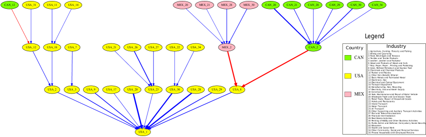
Figure 1: The GVT of USA’s agriculture industry in 2011. The edge weight threshold is set to 0.01 and the number of rounds is limited to 3. Different colors of the nodes indicate different countries. The red edges indicate cross-country relationships while the blue edges indicate domestic relationships. The edge width is proportional to the edge weight, i.e., the share of the value-added contribution.

Figure 1 shows the GVT of USA’s agriculture industry in 2011, with $\alpha=0.01$ and $\gamma=3$. The economic interpretation is that, if the final demand in the root is one million US dollars, then all the industries contributing more than 1% locally (to the direct neighbors) and directly or indirectly contributing more than 1 dollar (one million multiplied by ${0.01}^{3}$) to the root are included in the tree.

Insert Figure 1 here.

III Results

Once we have computed the GVTs, some basic properties of the tree topology can be explored. Subsection III.1 quantifies the allometric scaling pattern of the GVTs. We estimate the allometric scaling exponents and find that the GVTs are topologically more similar to a star than to a chain. However, the GVTs have become more and more hierarchical over time. Subsection III.2 proposes a tree-based industry importance measure and compares it with other network centrality measures. We find that the tree-based measure performs the best in terms of the correlation with the industry total value-added. Therefore, the GVTs still retain the essential information of the GVNs and can be viewed as a reasonable simplification of the latter.

III.1 Allometric Scaling Pattern

The allometric scaling pattern refers to the power law relationship between size and other physical or behavioral variables. Previous studies have documented the ubiquitous existence of the allometric scaling pattern in systems as diverse as river networks, cellular metabolism, population dynamics, and food web banavar1999size ; garlaschelli2003universal .

For a directed tree topology, if we denote the total number of nodes in the sub-tree rooted at node $i$ by $X_{i}$ and the sum of all $X_{i}$’s in the sub-tree rooted at node $i$ by $Y_{i}$, then an allometric scaling relationship is observed between $Y_{i}$ and $X_{i}$ and can be described by a power law, i.e., $Y_{i}\sim X_{i}^{\eta}$, where $\eta$ is called the allometric scaling exponent.

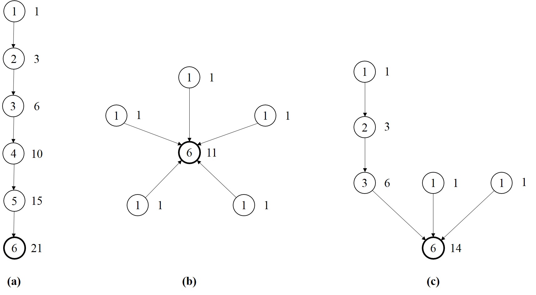
Figure 2: Examples of the allometric scaling relationship. The numbers inside the node circles are $X_{i}$’s whereas those next to the circles are $Y_{i}$’s. The node with the thick circle is the root. From left to right, they are a chain (a), a star (b), and a tree (c), respectively.

Figure 2 shows the examples of a chain, a star, and a tree, respectively. The numbers inside the node circles are $X_{i}$’s whereas those next to the circles are $Y_{i}$’s. The allometric scaling exponent $\eta$ of a tree is lower-bounded by that of a star ($\eta=1$) and upper-bounded by that of a chain ($\eta=2$). As a result, $\eta$ can be interpreted as a measure of hierarchicality, as star is the “flattest” topology and chain is the most hierarchical topology given the same number of nodes.

Insert Figure 2 here.

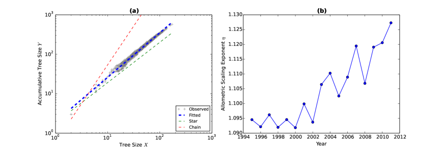
Figure 3: Estimation of the allometric scaling exponent $\eta$. Panel (a) shows the log-log plot of the root-node $Y_{i}$-$X_{i}$ pairs in 2011, where the horizontal axis is the $X_{i}$ of the root node, i.e., the total number of nodes in a given GVT (the tree size), and the vertical axis is the $Y_{i}$ of the root node, which we call the accumulative tree size. The gray crosses are the observed data points. The thick blue dashed line is fitted with the observed data and with the slope of $\eta$. The fitting lines for star and chain based on the same set of $X_{i}$’s are the green dashed line and the red dashed line respectively. Panel (b) plots the estimated $\eta$’s over time.

To examine the hierarchicality of the GVTs, we estimate $\eta$’s based on the root-node $Y_{i}$-$X_{i}$ pairs across all the GVTs for each year. Figure 3 has the estimation result of $\eta$. Panel (a) shows the log-log plot of the root-node $Y_{i}$-$X_{i}$ pairs in 2011, where the horizontal axis is the $X_{i}$ of the root node, i.e., the total number of nodes in a given GVT (the tree size), and the vertical axis is the $Y_{i}$ of the root node, which we call the accumulative tree size. The gray crosses are the observed data points. The thick blue dashed line is fitted with the observed data and with the slope of $\eta$. The fitting lines for star and chain based on the same set of $X_{i}$’s are the green dashed line and the red dashed line respectively. It is straightforward to see that in 2011 the GVTs are more similar to a star than to a chain. Panel (b) plots the estimated $\eta$’s over time. Again, the values of $\eta$ are all closer to 1 than to 2. However, there is a clear upward trend, which means that the GVTs have become more and more hierarchical over time (Shi et al. shi2014hierarchicality also estimate the allometric scaling exponent to understand the hierarchicality of the global production system. However, they consider the directed tree as a flow network. Furthermore, their paper differs from ours in both data source and research strategy. They use the United Nations COMTRADE database to construct the product-specific trade networks while we use the WIOD database to construct the GVNs with both country and industry dimensions.).

Insert Figure 3 here.

III.2 A Tree-Based Importance Measure

The GVTs are the subgraphs of the GVNs. Unlike the GVNs, the GVTs reveal the local importance of the industries. Previous studies have shown that the subgraph centrality measure can be used to complement the global centrality measures estrada2005subgraph . Hence, we compute a simple industry importance measure based on the GVTs and compare it with other network centrality measures.

First, we denote a tree with the root $r$ by $T(r)$. Furthermore, we denote the total number of nodes in the sub-tree rooted at industry $i$ by $X_{i}(r)$ and the total number of nodes in the tree $T(r)$ by $N(r)$. If industry $i$ is present in $k$ trees all over the world and we denote the set of roots of the $k$ trees by $S_{i}$, then the importance of industry $i$ is defined as follows:

$$TI_{i}=\sum_{r\in S_{i},r\neq i}\frac{X_{i}(r)}{N(r)}\frac{FD(r)}{WGDP}$$ (3)

where $TI_{i}$ is the tree-based importance measure of industry $i$, $FD(r)$ is the final demand in the root industry $r$ and $WGDP$ is the world GDP. Notice that when calculating $TI_{i}$, we don’t consider the role played by industry $i$ in its own GVT (i.e., $r\neq i$), although the input-output network has strong self-loops cerina2014world .

The economic interpretation of the importance measure is that, more important industries are more closely attached to the root and are able to “pull” a larger portion of the GVTs (measured by $\frac{X_{i}(r)}{N(r)}$) and are associated with more important roots (measured by $\frac{FD(r)}{WGDP}$).

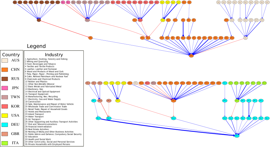
Figure 4: The domestic and foreign GVTs where China’s electrical equipment industry has the highest importance score in 2011. The upper and lower trees are the domestic and foreign trees respectively where China’s electrical equipment industry has the highest importance score. The edge weight threshold is set to 0.01 and the number of rounds is limited to 3. Different colors of the nodes indicate different countries. The red edges indicate cross-country relationships while the blue edges indicate domestic relationships. The edge width is proportional to the edge weight, i.e., the share of the value-added contribution.

Moreover, since each $T(r)$ where industry $i$ is present has a score of importance, i.e.,$\frac{X_{i}(r)}{N(r)}\frac{FD(r)}{WGDP}$, we can identify the GVTs where industry $i$ has the highest importance score. For instance, Figure 4 shows the GVTs where China’s electrical equipment industry has the highest importance score for domestic and foreign roots respectively in 2011.

Insert Figure 4 here.

To examine the tree-based importance measure in a more systematic way, we compare it with other network centrality measures. Table 3 has the top-20 industries identified by different measures for the selected years. Again, $TI$ is the tree-based importance measure. We also provide the results based on some network centrality measures. In particular, $CC$ is the closeness centrality, $BC$ is the betweenness centrality, $PR$ is the PageRank centrality. Finally, we include the measure of economic size of the industries, the industry total value-added, which is denoted by $VT$. Some interesting patterns can be seen from this table. First, all the measures have captured the rise of China over time. Back in 1995, almost no industries from China are identified as the top-20 (The only exception is that China’s construction industry takes the 19th place according to the PageRank centrality.). In 2003, China’s industries start to be picked up by $TI$, $BC$, and $PR$, which are more topologically sensitive than $CC$ and $VT$. In 2011, China’s industries show up in all the measures. Second, each measure captures different information, at least at the top-20 level. In 1995 and 2003, $VT$ is dominated by the service industries in big and advanced economies. But in 2011, the rise of China also brings the industries of agriculture and basic metals to the top list. $CC$ captures big industries in big economies (As shown later in Table 4, $log(CC)$ and $log(VT)$ are strongly correlated.). In 1995 $CC$ is mixed by USA and Germany while it is dominated by USA and China in 2003 and 2011 respectively. $BC$ has a more diverse list of industries in terms of economic size. Besides the big ones, it also includes smaller industries such as Turkey’s textiles industry and Indonesia’s mining industry. $PR$ is also diverse in terms of economic size. But it is quite stable over time, i.e., except for the rise of China, more or less the same industries are identified as the top-20. Last but not least, $TI$ generally identifies the big industries. But it also gives credits to industries such as Russia’s mining industry and Korea’s electrical equipment industry, which have strong presence in the GVTs (In Table S3 in Supplementary Information, we also report the country rankings by summing up the measures of the industries in the same country.).

Insert Table 3 here.

Moreover, Table 4 reports the Pearson correlation coefficients among them (in logarithm) for the selected years. For a given year, all the coefficients are based on a common sample among the different measures. It turns out that all the coefficients are positive and almost all of them are significant at 1% level (The only exceptions are between $log(BC)$ and $log(CC)$ in 2003 and 2011.).

We find that $TI$ performs the best in terms of the correlation with $VT$. Nevertheless, this is not to say that we should abandon other measures and solely use $TI$ to understand the importance of a given industry. After all, we only consider the intermediate value-added flows when calculating $CC$, $BC$, and $PR$, whereas we also take into account the final demand in the root industry, i.e., $FD(r)$, when calculating $TI$, which gives more power to $TI$ in explaining $VT$. However, the strong correlation between $log(TI)$ and $log(VT)$ at least shows that the GVTs retain the essential information of the GVNs and can be viewed as a reasonable simplification of the latter. That is, $TI$ can be considered as a measure of industry’s position advantage. An industry holds an advantageous position by either attaching to big industries (i.e., big $\frac{FD(r)}{WGDP}$) or by affecting big portion of the GVTs (i.e., big $\frac{X_{i}(r)}{N(r)}$). As a result, the better-positioned industries are more competitive in the world production system and hence are able to extract more value-added across the GVTs. Moreover, since the component $\frac{X_{i}(r)}{N(r)}$ of $TI$ measures how closely the given industry is attached to the roots (i.e., bigger $\frac{X_{i}(r)}{N(r)}$ implies smaller distance to the roots), it can be considered as a measure of downstreamness. That is, the higher $TI$ is the more downstream the industry is in the GVTs. Therefore, the strong correlation between $log(TI)$ and $log(VT)$ supports Stan Shih’s theory of “smiling curve”, which states that most value-added potentials are concentrated at the beginning (upstream) and the ending (downstream) parts of the supply chains.

Insert Table 4 here.

IV Discussion

Once we have the GVTs computed for all the industries available in the WIOD, many interesting questions can be proposed and answered. For instance, does a tree with a fixed root grow over time? This question can be answered by fixing the root industry and examining the GVTs over time. As an example, Figure 5 shows the evolution of the GVTs rooted at China’s electrical equipment industry over time. A simple way of measuring the growth of the trees is to count the number of nodes over time. In Figure 5, the GVT of China’s electrical equipment industry evolves from 47 nodes in 1995 to 100 nodes in 2003 and to 106 in 2011. There are also some interesting structural changes in this example. First, Australia’s mining industry (AUS_2) becomes directly attached to the root in 2011. Second, Japan’s electrical equipment industry (JPN_14) is a direct neighbor of the root in 2003 but has to go through Taiwan’s electrical equipment industry (TWN_14) in 2011. The structural changes may have important implications for the industries’ competitiveness. In particular, TWN_14 has become more competitive than JPN_14 with respect to China’s electrical equipment industry based on the $TI$ measure.

Insert Figure 5 here.

We can also examine the different structures of the GVTs for the same industry and the same year but for different countries. Figure 6 compares the transport equipment industry between Indonesia and Japan in 1995. The immediate conclusion from this comparison is that the transport equipment industry has a more international GVT in Indonesia than in Japan. More interestingly, Japan’s industries actually play important roles in Indonesia’s GVT, i.e., three Japan’s industries (JPN_12, JPN_15, and JPN_20) are direct neighbors of the root in Indonesia (This observation coincides with the increased foreign direct investment from Japan to Indonesia’s car industry in 1995.). In this simple comparison, JPN_15 is clearly more competitive than IDN_15, according to the above $TI$ measure.

Insert Figure 6 here.

In summary, previous studies of the GVCs are mainly interested in knowing how global the GVCs are rather than how the GVCs look like. To fill the gap in the literature, our paper is the first attempt to investigate the topological properties of the industry-level GVCs. From a complex networks perspective, we map the World Input-Output Database (WIOD) into the global value networks (GVNs), where the nodes are the individual industries in different countries and the edges are the value-added contribution relationships.

Based on the GVNs, the global value trees (GVTs) can be obtained by a breadth-first search algorithm with a threshold of edge weight and a limit of the number of rounds. We compute the GVTs for all the industries available in the WIOD and explore some basic properties of the GVTs. In particular, we estimate the allometric scaling exponents and find that the GVTs are topologically more similar to a star than to a chain. However, the GVTs have become more and more hierarchical over time. We also develop an industry importance measure based on the GVTs and compare it with other network centrality measures of the industries. We find that the tree-based measure performs the best in terms of the correlation with the industry total value-added. Therefore, the GVTs still retain the essential information of the GVNs and can be viewed as a reasonable simplification of the latter. Finally, we discuss some future applications of the GVTs such as to examine the evolution of the GVTs for a certain industry and to compare the GVTs of the same industry in different countries.

Author Contributions

A.C., M.P., M.R., and Z.Z. conceived and designed the research. F.C., M.P., and Z.Z. performed the computation. M.R. and Z.Z. analyzed the results. Z.Z. wrote the main text.

Additional Information

The authors declare no competing financial interests.

Figures

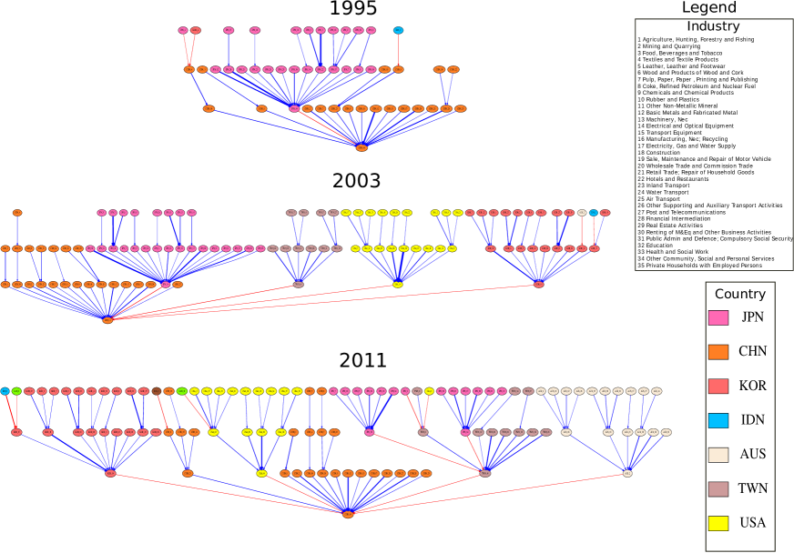
Figure 5: The evolution of the GVTs rooted at China’s electrical equipment industry. From top down, the GVTs are for 1995, 2003, and 2011 respectively. The edge weight threshold is set to 0.01 and the number of rounds is limited to 3. Different colors of the nodes indicate different countries. The red edges indicate cross-country relationships while the blue edges indicate domestic relationships. The edge width is proportional to the edge weight, i.e., the share of the value-added contribution.

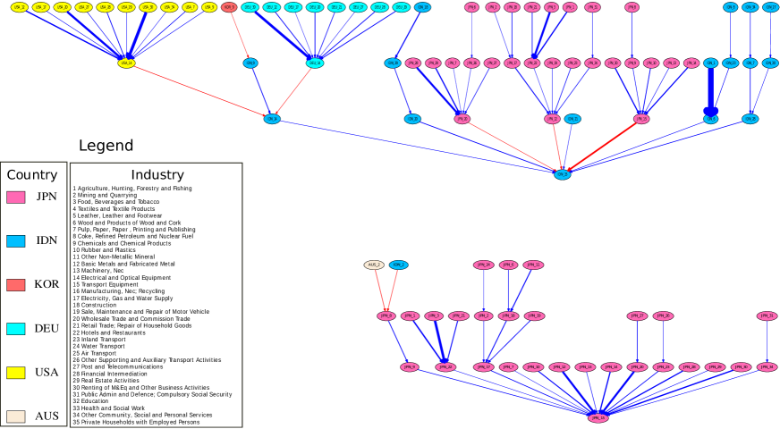
Figure 6: The comparison of the transport equipment industry between Indonesia and Japan in 1995. The upper and lower GVTs are rooted in the tranport equipment industry in Indonesia and Japan respectively in 1995. The edge weight threshold is set to 0.01 and the number of rounds is limited to 3. Different colors of the nodes indicate different countries. The red edges indicate cross-country relationships while the blue edges indicate domestic relationships. The edge width is proportional to the edge weight, i.e., the share of the value-added contribution.

Tables

Table 1: A hypothetical two-economy-two-industry MRIO table. The $4\times 4$ inter-industry transactions matrix records outputs selling in its rows and inputs buying in its columns. The additional columns are the final demand and the additional row is the value added. Finally, the last column and the last row record the total industry outputs.

		Buyer Industry
		Economy 1		Economy 2		Final Demand
Seller Industry		Industry 1	Industry 2	Industry 1	Industry 2	Economy 1	Economy 2	Total Output
Economy 1	Industry 1	25	10	20	10	45	10	120
	Industry 2	10	5	10	20	50	5	100
Economy 2	Industry 1	30	15	600	500	5	8650	9800
	Industry 2	35	30	1000	1000	25	7910	10000
Value Added		20	40	8170	8470
Total Output		120	100	9800	10000

Table 2: The summary statistics of the size of the GVTs by varying the weight threshold, i.e., $\alpha$, for the selected years. The number of observations is the number of nonempty GVTs according to the value of $\alpha$. CV stands for the coefficient of variation, which is the standard deviation divided by the mean.

	$\alpha=0.1$			$\alpha=0.01$			$\alpha=0.001$
	1995	2003	2011	1995	2003	2011	1995	2003	2011
# Obs.	182	184	194	1344	1345	1342	1348	1347	1345
Min	2	2	2	9	2	2	196	173	159
Max	4	4	5	149	221	172	1165	1150	1162
Mean	2.104	2.076	2.062	48.089	43.888	44.242	793.677	856.200	855.436
CV	0.162	0.147	0.145	0.489	0.527	0.531	0.194	0.198	0.197

Table 3: The top-20 industries identified by the tree-based importance measure and other network centrality measures for the selected years. $TI$ is the tree-based importance measure, $CC$ is the closeness centrality, $BC$ is the betweenness centrality, $PR$ is the PageRank centrality, $VT$ is the industry total value-added. The full names of the corresponding industries of the 3-letter codes can be found in Table S2 in Supplementary Information.

	1995					2003					2011
Rank	$TI$	$CC$	$BC$	$PR$	$VT$	$TI$	$CC$	$BC$	$PR$	$VT$	$TI$	$CC$	$BC$	$PR$	$VT$
1	USA-Pup	DEU-Tpt	USA-Obs	USA-Pub	USA-Pub	USA-Cst	USA-Obs	USA-Obs	USA-Pub	USA-Obs	USA-Obs	CHN-Cst	CHN-Cst	USA-Pub	USA-Obs
2	CAN-Pup	DEU-Obs	DEU-Obs	USA-Cst	USA-Est	USA-Obs	USA-Tpt	DEU-Tpt	USA-Hth	USA-Pub	USA-Htl	CHN-Met	USA-Pub	CHN-Cst	USA-Pub
3	USA-Cst	DEU-Est	USA-Pub	USA-Hth	USA-Obs	USA-Est	USA-Pub	USA-Tpt	USA-Cst	USA-Est	USA-Cst	CHN-Omn	USA-Obs	USA-Hth	USA-Est
4	USA-Obs	DEU-Cst	USA-Elc	JPN-Cst	USA-Rtl	USA-Htl	USA-Hth	DEU-Obs	USA-Est	USA-Fin	CHN-Elc	CHN-Min	RUS-Min	CHN-Pub	USA-Fin
5	JPN-Ele	DEU-Elc	DEU-Tpt	USA-Est	USA-Fin	USA-Ele	USA-Fin	USA-Pub	USA-Tpt	USA-Rtl	AUS-Min	CHN-Whl	DEU-Obs	DEU-Tpt	USA-Hth
6	USA-Est	DEU-Fod	RUS-Min	USA-Tpt	JPN-Est	USA-Cok	USA-Cst	DEU-Cok	CHN-Cst	USA-Hth	RUS-Min	CHN-Elc	DEU-Tpt	CHN-Elc	USA-Rtl
7	GBR-Fin	USA-Obs	FRA-Obs	USA-Htl	USA-Whl	USA-Wod	USA-Est	JPN-Tpt	DEU-Tpt	USA-Whl	USA-Ocm	CHN-Fin	CHN-Elc	USA-Cst	USA-Whl
8	DEU-Fin	USA-Pub	JPN-Elc	USA-Rtl	USA-Hth	GBR-Fin	USA-Rtl	DEU-Elc	USA-Htl	USA-Cst	JPN-Ele	CHN-Ldt	CHN-Agr	CHN-Hth	JPN-Est
9	JPN-Elc	FRA-Obs	USA-Fod	DEU-Cst	JPN-Whl	USA-Pup	USA-Whl	USA-Elc	USA-Rtl	JPN-Est	USA-Met	CHN-Agr	GBR-Obs	USA-Htl	CHN-Agr
10	USA-Elc	DEU-Hth	DEU-Met	USA-Fod	JPN-Cst	USA-Ldt	USA-Ocm	USA-Fod	USA-Ocm	USA-Ocm	USA-Otr	CHN-Ele	ESP-Obs	USA-Tpt	USA-Ocm
11	USA-Ele	DEU-Met	USA-Tpt	DEU-Tpt	USA-Cst	USA-Chm	USA-Htl	JPN-Whl	USA-Fod	USA-Htl	USA-Whl	CHN-Chm	FIN-Obs	USA-Rtl	USA-Cst
12	USA-Ldt	USA-Elc	JPN-Whl	DEU-Fod	JPN-Fin	USA-Met	USA-Fod	RUS-Min	GBR-Pub	JPN-Pub	USA-Cok	CHN-Fod	USA-Fin	USA-Est	CHN-Whl
13	JPN-Cst	USA-Whl	JPN-Cst	USA-Ocm	JPN-Pub	CAN-Min	USA-Elc	JPN-Cst	JPN-Cst	JPN-Whl	USA-Ele	CHN-Obs	USA-Cok	CHN-Mch	JPN-Pub
14	JPN-Sal	USA-Tpt	DEU-Elc	JPN-Pub	JPN-Obs	DEU-Fin	USA-Pst	CHN-Elc	DEU-Fod	JPN-Obs	USA-Min	CHN-Pst	CHN-Tex	CHN-Tpt	CHN-Cst
15	JPN-Ldt	USA-Hth	DEU-Tex	DEU-Hth	JPN-Rtl	USA-Otr	DEU-Tpt	DEU-Met	DEU-Cst	USA-Pst	USA-Fin	CHN-Mch	DEU-Met	USA-Fod	USA-Htl
16	USA-Chm	USA-Cst	DEU-Cok	GBR-Pub	USA-Ocm	JPN-Ele	USA-Met	ESP-Tpt	CHN-Pub	DEU-Obs	CAN-Min	CHN-Otr	FIN-Cst	USA-Ocm	JPN-Obs
17	USA-Htl	USA-Fin	FRA-Ele	DEU-Htl	DEU-Est	USA-Whl	USA-Agr	FRA-Obs	GBR-Est	JPN-Cst	CHN-Obs	USA-Obs	TUR-Tex	GBR-Hth	DEU-Obs
18	JPN-Cok	USA-Rtl	DEU-Cst	DEU-Est	DEU-Obs	CHN-Elc	USA-Pup	ITA-Obs	FRA-Tpt	DEU-Est	USA-Pub	USA-Pub	FRA-Obs	CHN-Fod	JPN-Whl
19	DEU-Cst	USA-Est	JPN-Met	CHN-Cst	JPN-Ocm	DEU-Met	USA-Chm	CHN-Cst	USA-Fin	JPN-Fin	GBR-Fin	USA-Hth	AUS-Min	CHN-Edu	CHN-Est
20	JPN-Htl	DEU-Fin	DEU-Fod	FRA-Tpt	USA-Pst	JPN-Sal	DEU-Obs	USA-Agr	ESP-Cst	GBR-Obs	USA-Fod	CHN-Wod	IDN-Min	JPN-Cst	CHN-Met

Table 4: The Pearson correlation coefficient matrix between the tree-based importance measure and other network centrality measures (in logarithm) for the selected years. The size of the sample is in the parentheses next to the corresponding years. $TI$ is the tree-based importance measure, $CC$ is the closeness centrality, $BC$ is the betweenness centrality, $PR$ is the PageRank centrality, $VT$ is the industry total value-added. $\ast\ast$ means that the coefficient is significant at 1% level. $\ast$ means that the coefficient is significant at 5% level.

1995 (# Obs. 384)						2003 (# Obs. 351)						2011 (# Obs. 324)
	$log(TI)$	$log(CC)$	$log(BC)$	$log(PR)$	$log(VT)$		$log(TI)$	$log(CC)$	$log(BC)$	$log(PR)$	$log(VT)$		$log(TI)$	$log(CC)$	$log(BC)$	$log(PR)$	$log(VT)$
$log(TI)$	1	-	-	-	-	$log(TI)$	1	-	-	-	-	$log(TI)$	1	-	-	-	-
$log(CC)$	0.577$\ast\ast$	1	-	-	-	$log(CC)$	0.560$\ast\ast$	1	-	-	-	$log(CC)$	0.523$\ast\ast$	1	-	-	-
$log(BC)$	0.282$\ast\ast$	0.196$\ast\ast$	1	-	-	$log(BC)$	0.229$\ast\ast$	0.063	1	-	-	$log(BC)$	0.276$\ast\ast$	0.082	1	-	-
$log(PR)$	0.436$\ast\ast$	0.363$\ast\ast$	0.370$\ast\ast$	1	-	$log(PR)$	0.450$\ast\ast$	0.395$\ast\ast$	0.317$\ast\ast$	1	-	$log(PR)$	0.388$\ast\ast$	0.328$\ast\ast$	0.235$\ast\ast$	1	-
$log(VT)$	0.838$\ast\ast$	0.703$\ast\ast$	0.325$\ast\ast$	0.663$\ast\ast$	1	$log(VT)$	0.814$\ast\ast$	0.727$\ast\ast$	0.256$\ast\ast$	0.684$\ast\ast$	1	$log(VT)$	0.820$\ast\ast$	0.639$\ast\ast$	0.276$\ast\ast$	0.623$\ast\ast$	1

Supplementary Information

Table S1: The list of WIOD economies.

Euro-Zone		Non-Euro EU		NAFTA		East Asia		BRIIAT
Economy	3L Code	Economy	3L Code	Economy	3L Code	Economy	3L Code	Economy	3L Code
Austria	AUT	Bulgaria	BGR	Canada	CAN	China	CHN	Australia	AUS
Belgium	BEL	Czech Rep.	CZE	Mexico	MEX	Japan	JPN	Brazil	BRA
Cyprus	CYP	Denmark	DNK	USA	USA	South Korea	KOR	India	IND
Estonia	EST	Hungary	HUN			Taiwan	TWN	Indonesia	IDN
Finland	FIN	Latvia	LVA					Russia	RUS
France	FRA	Lithuania	LTU					Turkey	TUR
Germany	DEU	Poland	POL
Greece	GRC	Romania	ROM
Ireland	IRL	Sweden	SWE
Italy	ITA	UK	GBR
Luxembourg	LUX
Malta	MLT
Netherlands	NLD
Portugal	PRT
Slovakia	SVK
Slovenia	SVN
Spain	ESP

Table S2: The list of WIOD industries.

Full Name	ISIC Rev. 3 Code	WIOD Code	3-Letter Code
Agriculture, Hunting, Forestry and Fishing	AtB	c1	Agr
Mining and Quarrying	C	c2	Min
Food, Beverages and Tobacco	15t16	c3	Fod
Textiles and Textile Products	17t18	c4	Tex
Leather, Leather and Footwear	19	c5	Lth
Wood and Products of Wood and Cork	20	c6	Wod
Pulp, Paper, Paper , Printing and Publishing	21t22	c7	Pup
Coke, Refined Petroleum and Nuclear Fuel	23	c8	Cok
Chemicals and Chemical Products	24	c9	Chm
Rubber and Plastics	25	c10	Rub
Other Non-Metallic Mineral	26	c11	Omn
Basic Metals and Fabricated Metal	27t28	c12	Met
Machinery, Nec	29	c13	Mch
Electrical and Optical Equipment	30t33	c14	Elc
Transport Equipment	34t35	c15	Tpt
Manufacturing, Nec; Recycling	36t37	c16	Mnf
Electricity, Gas and Water Supply	E	c17	Ele
Construction	F	c18	Cst
Sale, Maintenance and Repair of Motor Vehicles and Motorcycles; Retail Sale of Fuel	50	c19	Sal
Wholesale Trade and Commission Trade, Except of Motor Vehicles and Motorcycles	51	c20	Whl
Retail Trade, Except of Motor Vehicles and Motorcycles; Repair of Household Goods	52	c21	Rtl
Hotels and Restaurants	H	c22	Htl
Inland Transport	60	c23	Ldt
Water Transport	61	c24	Wtt
Air Transport	62	c25	Ait
Other Supporting and Auxiliary Transport Activities; Activities of Travel Agencies	63	c26	Otr
Post and Telecommunications	64	c27	Pst
Financial Intermediation	J	c28	Fin
Real Estate Activities	70	c29	Est
Renting of M&Eq and Other Business Activities	71t74	c30	Obs
Public Admin and Defence; Compulsory Social Security	L	c31	Pub
Education	M	c32	Edu
Health and Social Work	N	c33	Hth
Other Community, Social and Personal Services	O	c34	Ocm
Private Households with Employed Persons	P	c35	Pvt

Table S3: The country rankings based on the tree-based importance measure and other network centrality measures for the selected years. $TI$ is the tree-based importance measure, $CC$ is the closeness centrality, $BC$ is the betweenness centrality, $PR$ is the PageRank centrality, $VT$ is the industry total value-added. The full names of the corresponding industries of the 3-letter codes can be found in Table S2 in Supplementary Information.

	1995					2003					2011
Rank	$TI$	$CC$	$BC$	$PR$	$VT$	$TI$	$CC$	$BC$	$PR$	$VT$	$TI$	$CC$	$BC$	$PR$	$VT$
1	USA	USA	DEU	USA	USA	USA	USA	USA	USA	USA	USA	USA	CHN	USA	USA
2	JPN	FRA	USA	DEU	JPN	JPN	FRA	DEU	DEU	JPN	CHN	FRA	USA	CHN	CHN
3	DEU	CAN	JPN	JPN	DEU	DEU	MEX	JPN	GBR	DEU	JPN	CAN	DEU	DEU	JPN
4	GBR	MEX	FRA	GBR	FRA	GBR	CAN	CHN	CHN	GBR	AUS	MEX	RUS	GBR	DEU
5	CAN	GBR	RUS	ITA	GBR	FRA	GBR	ITA	ITA	FRA	DEU	GBR	ESP	ITA	FRA
6	FRA	TWN	ITA	FRA	ITA	CAN	DEU	ESP	JPN	CHN	RUS	JPN	GBR	FRA	GBR
7	ITA	DEU	GBR	ESP	CHN	CHN	JPN	RUS	FRA	ITA	CAN	DEU	FIN	JPN	BRA
8	BRA	JPN	ESP	KOR	BRA	ITA	ITA	FRA	ESP	ESP	GBR	BRA	KOR	RUS	ITA
9	AUS	ITA	FIN	CHN	ESP	RUS	ESP	FIN	KOR	CAN	FRA	ITA	AUS	ESP	IND
10	RUS	KOR	AUS	GRC	CAN	MEX	KOR	GBR	TUR	MEX	ITA	RUS	BRA	BRA	CAN
11	ESP	ESP	BRA	BRA	KOR	ESP	IND	IND	CAN	KOR	BRA	IND	JPN	CAN	ESP
12	CHN	AUS	ROM	RUS	NLD	AUS	AUS	TUR	MEX	IND	IND	AUS	FRA	IND	AUS
13	KOR	BRA	DNK	AUS	IND	KOR	NLD	AUS	GRC	BRA	KOR	KOR	CAN	TUR	RUS
14	IND	NLD	IDN	TUR	AUS	IND	BRA	IDN	AUS	AUS	MEX	ESP	ITA	KOR	MEX
15	IDN	RUS	KOR	NLD	RUS	BRA	TWN	BRA	RUS	NLD	ESP	TUR	IDN	AUS	KOR
16	NLD	IND	BEL	IND	MEX	NLD	RUS	DNK	IND	RUS	TWN	TWN	TUR	GRC	IDN
17	MEX	BEL	IND	CAN	BEL	TWN	BEL	POL	NLD	TWN	IDN	NLD	MEX	MEX	NLD
18	SWE	DNK	TUR	SWE	TWN	IDN	TUR	HUN	SWE	BEL	TUR	BEL	GRC	POL	TUR
19	BEL	SWE	CHN	AUT	IDN	TUR	SWE	BGR	BRA	SWE	NLD	POL	LVA	IDN	SWE
20	TUR	POL	MEX	BEL	SWE	SWE	POL	ROM	POL	TUR	SWE	FIN	CZE	NLD	BEL
21	TWN	FIN	BGR	DNK	AUT	BEL	GRC	CAN	AUT	IDN	POL	GRC	HUN	SWE	POL
22	AUT	AUT	GRC	PRT	TUR	DNK	DNK	KOR	BEL	AUT	BEL	PRT	POL	BEL	TWN
23	DNK	PRT	NLD	TWN	DNK	AUT	PRT	SVK	IDN	POL	DNK	AUT	IND	FIN	AUT
24	GRC	GRC	CAN	MEX	POL	POL	AUT	GRC	FIN	DNK	AUT	DNK	SVK	AUT	DNK
25	POL	CZE	LVA	FIN	GRC	GRC	FIN	TWN	DNK	GRC	GRC	IRL	CYP	ROM	GRC
26	FIN	IRL	HUN	IDN	FIN	FIN	IRL	PRT	PRT	FIN	PRT	ROM	SWE	DNK	FIN
27	PRT	CHN	PRT	POL	PRT	PRT	CHN	EST	IRL	IRL	FIN	CZE	ROM	PRT	PRT
28	CZE	IDN	POL	CZE	IRL	IRL	CZE	BEL	CZE	PRT	ROM	HUN	PRT	CZE	IRL
29	ROM	ROM	SWE	HUN	CZE	CZE	IDN	CZE	HUN	CZE	CZE	SVK	DNK	CYP	CZE
30	HUN	TUR	TWN	ROM	HUN	HUN	HUN	LVA	CYP	HUN	HUN	BGR	SVN	HUN	ROM
31	IRL	HUN	AUT	CYP	ROM	ROM	ROM	SWE	TWN	ROM	IRL	CHN	BEL	TWN	HUN
32	SVN	SVN	CYP	IRL	LUX	SVN	SVK	CYP	ROM	SVK	SVK	IDN	BGR	IRL	SVK
33	SVK	BGR	CZE	SVN	SVN	SVK	SVN	MEX	SVN	LUX	SVN	SWE	MLT	BGR	LUX
34	BGR	SVK	LTU	BGR	SVK	BGR	LTU	LTU	LTU	SVN	BGR	LTU	LUX	SVK	BGR
35	CYP	LUX	SVN	LVA	BGR	LTU	BGR	MLT	LVA	BGR	CYP	SVN	LTU	LVA	SVN
36	LUX	LTU	IRL	LTU	CYP	CYP	LUX	NLD	SVK	LTU	LTU	EST	EST	LTU	LTU
37	LTU	CYP	EST	SVK	LTU	LUX	CYP	SVN	BGR	CYP	LVA	LVA	TWN	SVN	LVA
38	LVA	EST	SVK	EST	LVA	LVA	LVA	AUT	EST	LVA	EST	LUX	NLD	EST	CYP
39	EST	MLT	MLT	MLT	EST	EST	EST	IRL	MLT	EST	LUX	CYP	AUT	MLT	EST
40	MLT	LVA	LUX	LUX	MLT	MLT	MLT	LUX	LUX	MLT	MLT	MLT	IRL	LUX	MLT

References

- (1) Baldwin, R. Globalisation: the great unbundling(s). Tech. Rep., Economic Council of Finland (2006).
- (2) Baldwin, R. & Lopez-Gonzalez, J. Supply-chain trade: a portrait of global patterns and several testable hypotheses. World Economy (2014).
- (3) Costinot, A., Vogel, J. & Wang, S. An elementary theory of global supply chains. Review of Economic Studies 80, 109–144 (2013).
- (4) Los, B., Timmer, M. P. & Vries, G. J. How global are global value chains? a new approach to measure international fragmentation. Journal of Regional Science (2014).
- (5) Feenstra, R. C. & Hanson, G. H. The impact of outsourcing and high-technology capital on wages: estimates for the United States, 1979-1990. Quarterly Journal of Economics 907–940 (1999).
- (6) Grossman, G. M. & Rossi-Hansberg, E. Trading tasks: a simple theory of offshoring. American Economic Review 98, 1978–1997 (2008).
- (7) Hummels, D., Ishii, J. & Yi, K.-M. The nature and growth of vertical specialization in world trade. Journal of International Economics 54, 75–96 (2001).
- (8) Dedrick, J., Kraemer, K. L. & Linden, G. Who profits from innovation in global value chains?: a study of the iPod and notebook PCs. Industrial and Corporate Change 19, 81–116 (2010).
- (9) Baldwin, R. & Venables, A. J. Spiders and snakes: offshoring and agglomeration in the global economy. Journal of International Economics 90, 245–254 (2013).
- (10) Johnson, R. C. & Noguera, G. Accounting for intermediates: production sharing and trade in value added. Journal of International Economics 86, 224–236 (2012).
- (11) Johnson, R. C. Five facts about value-added exports and implications for macroeconomics and trade research. Journal of Economic Perspectives 28, 119–142 (2014).
- (12) Timmer, M. P., Erumban, A. A., Los, B., Stehrer, R. & de Vries, G. J. Slicing up global value chains. Journal of Economic Perspectives 28, 99–118 (2014).
- (13) Amador, J. & Cabral, S. Global value chains: a survey of drivers and measures. Journal of Economic Surveys (2014).
- (14) Antràs, P., Chor, D., Fally, T. & Hillberry, R. Measuring the upstreamness of production and trade flows. American Economic Review 102, 412–416 (2012).
- (15) Backer, K. & Miroudot, S. Mapping global value chains. Tech. Rep., OECD Publishing (2013).
- (16) Timmer, M. et al. The world input-output database (WIOD): contents, sources and methods. Tech. Rep., (2012).
- (17) Kitsak, M., Riccaboni, M., Havlin, S., Pammolli, F. & Stanley, H. E. Scale-free models for the structure of business firm networks. Physical Review E 81, 036117 (2010).
- (18) Pammolli, F. & Riccaboni, M. Technological regimes and the growth of networks: an empirical analysis. Small Business Economics 19, 205–215 (2002).
- (19) Riccaboni, M. & Schiavo, S. Structure and growth of weighted networks. New Journal of Physics 12, 023003 (2010).
- (20) Riccaboni, M., Rossi, A. & Schiavo, S. Global networks of trade and bits. Journal of Economic Interaction and Coordination 8, 33–56 (2013).
- (21) Chessa, A. et al. Is Europe evolving toward an integrated research area? Science 339, 650–651 (2013).
- (22) Caldarelli, G., Chessa, A., Pammolli, F., Gabrielli, A. & Puliga, M. Reconstructing a credit network. Nature Physics 9, 125–126 (2013).
- (23) Zhu, Z., Cerina, F., Chessa, A., Caldarelli, G. & Riccaboni, M. The rise of China in the international trade network: a community core detection approach. PLoS ONE 9, e105496 (2014).
- (24) Cerina, F., Zhu, Z., Chessa, A. & Riccaboni, M. World input-output network. arXiv preprint arXiv:1407.0225 (2014).
- (25) Sturgeon, T. J. How do we define value chains and production networks? IDS Bulletin 32, 9–18 (2001).
- (26) Coe, N. M., Hess, M., Yeung, H. W.-c., Dicken, P. & Henderson, J. Globalizing regional development: a global production networks perspective. Transactions of the Institute of British Geographers 29, 468–484 (2004).
- (27) Coe, N. M., Dicken, P. & Hess, M. Global production networks: realizing the potential. Journal of Economic Geography 8, 271–295 (2008).
- (28) Sturgeon, T., Van Biesebroeck, J. & Gereffi, G. Value chains, networks and clusters: reframing the global automotive industry. Journal of Economic Geography 8, 297–321 (2008).
- (29) Leontief, W. W. Quantitative input and output relations in the economic systems of the United States. Review of Economic Statistics 105–125 (1936).
- (30) Miller, R. E. & Blair, P. D. Input-Output Analysis: Foundations and Extensions (Cambridge University Press, 2009).
- (31) Banavar, J. R., Maritan, A. & Rinaldo, A. Size and form in efficient transportation networks. Nature 399, 130–132 (1999).
- (32) Garlaschelli, D., Caldarelli, G. & Pietronero, L. Universal scaling relations in food webs. Nature 423, 165–168 (2003).
- (33) Shi, P., Zhang, J., Yang, B. & Luo, J. Hierarchicality of trade flow networks reveals complexity of products. PloS ONE 9, e98247 (2014).
- (34) Estrada, E. & Rodriguez-Velazquez, J. A. Subgraph centrality in complex networks. Physical Review E 71, 056103 (2005).