Self-consistent field model for strong electrostatic correlations and
inhomogeneous dielectric media

Abstract

Electrostatic correlations and variable permittivity of electrolytes are essential for exploring many chemical and physical properties of interfaces in aqueous solutions. We propose a continuum electrostatic model for the treatment of these effects in the framework of the self-consistent field theory. The model incorporates a space- or field-dependent dielectric permittivity and an excluded ion-size effect for the correlation energy. This results in a self-energy modified Poisson-Nernst-Planck or Poisson-Boltzmann equation together with state equations for the self energy and the dielectric function. We show that the ionic size is of significant importance in predicting a finite self energy for an ion in an inhomogeneous medium. Asymptotic approximation is proposed for the solution of a generalized Debye-Hückel equation, which has been shown to capture the ionic correlation and dielectric self energy. Through simulating ionic distribution surrounding a macroion, the modified self-consistent field model is shown to agree with particle-based Monte Carlo simulations. Numerical results for symmetric and asymmetric electrolytes demonstrate that the model is able to predict the charge inversion at high correlation regime in the presence of multivalent interfacial ions which is beyond the mean-field theory, and also show strong effect to double layer structure due to the space- or field-dependent dielectric permittivity.

I Introduction

Electrostatic interaction in aqueous solutions including charged interfaces is of interest in a wide range of areas such as biological macromolecules, colloidal suspensions and nanoparticle assembly. The structure of screened ions near charged surfaces, so-called the electric double layer, controls many macroscopic properties of the system such as the zeta potential and colloidal renormalized charges Levin (2002); Hunter (1981); Joly et al. (2004); French et al. (2010); Walker et al. (2011), and is affected by the interfacial chemistry, the surface charge distribution, the ionic specificity, and so on. In the presence of divalent ions, electrostatic correlation plays a very important role, which could lead to the overscreening of counterions near highly charged surfaces, i.e., the charge inversion phenomenon Besteman et al. (2004); Pittler et al. (2006); Lozada-Cassou et al. (1982); Deserno et al. (2001); Grosberg et al. (2002). The electrostatic correlation is probably responsible for a lot of many-body phenomena such as like-charge attraction Larsen and Grier (1997); Angelini et al. (2003) and ion crowding in membrane channels Eisenberg (2011), and many-body systems such as electrodes in ionic liquids Fedorov and Kornyshev (2014). The correct understanding of correlation effects and their relation with interfacial properties are then considered to be of significant in many applications.

Electrostatic correlation should be seriously studied in many conditions, e.g., if a system includes highly charged surfaces, multivalent counterions, or if the system is at low temperature. The correlation strength is often measured by a coupling parameter Boroudjerdi et al. (2005) defined as $\Xi=z_{c}^{3}\sigma e^{4}/8\pi(\varepsilon k_{B}T)^{2},$ where $z_{c}$, $\sigma$, $e$, $\varepsilon$ and $k_{B}T$ are the counterion valence, the average surface charge density, the electronic charge, the dielectric permittivity, and the thermal energy, respectively. The coupling parameter can be simplified to $\Xi=z_{c}^{2}\ell_{B}/\ell_{GC}$, the product of $z_{c}^{2}$ and the ratio of the Bjerrum length $\ell_{B}$ to the Gouy-Chapman length $\ell_{GC}$. These two length scales describe the ion-ion and ion-interface interaction strengths, respectively. The classical Poisson-Boltzmann (PB) theory is often used, but it is mean-field and works only when $\Xi\ll 1$ since it ignores the ion correlation, thus fails to capture correlation-induced electrostatic phenomena. Many extended theories beyond the mean field have been proposed and applied for different problems, e.g., to include the steric effect or dielectric self energy Borukhov et al. (1997); Kilic et al. (2007); Corry et al. (2003); Graf et al. (2004); Eisenberg et al. (2010). A first-principle description of electrostatic correlation should follow the integral-equation theory Hansen and McDonald (2006), which turns out to be a difficulty in resolving high-dimensional obstacles. Phenomenologically, the electrostatic correlation is taken into account in a Ginzburg-Laudau-type functional which yields a modified PB equation with a biharmonic term to describe the contribution from the correlation energy Bazant et al. (2011); Liu and Eisenberg (2013) and a correlation length as a parameter to be accurately fitted by simulations or experiments.

In most of theoretical and computational studies under the primitive model Linse (2005); Messina (2009), a homogeneous dielectric profile for electrolytes near surfaces is often assumed, e.g., 80 for the relative dielectric constant of water solvent. This is far from a high-accurate description of the solvent. Water molecules are ordered near micro- or macro- ions, weakening the shielding for ion-ion interactions. This has led to models for ion-concentration- or field-dependent dielectric permittivities. Historically, the dependence of the dielectric permittivity on the ionic solution has been discussed as early as 1940s Hasted et al. (1948). Later, Booth considered the dielectric constant of polar electrolytes as a function of the electrostatic field strength Booth (1951, 1955), which was followed by many related studies from molecular dynamics simulations Yeh and Berkowitz (1999); Fulton (2009) to continuum theory Gur et al. (1978); Paunov et al. (1996). Recent work also reported that the dielectric decrement is relevant to ion-specific effects Ben-Yaakov et al. (2011). On the other hand, the Booth’s model was utilized to modify the Poisson-Boltzmann equation to predict the capacitance with effects of morphology and dielectric permittivity Wang et al. (2011). Coupled with the Booth’s model, the Langevin-Poisson-Boltzmann (LPB) equation was developed to investigate the effects of polarization saturation to the contact potential at the colloid surface and the long-range interaction between colloids Frydel and Oettel (2011). More recently, Bonthuis et al. Bonthuis et al. (2011, 2012) and Bonthuis and Netz Bonthuis and Netz (2013) through molecular dynamics simulations showed that the interfacial dielectric function is closely related to the molecular solvent structure of the surface. By incorporating the structure properties in the dielectric profile, the Bonthuis-Netz model Bonthuis and Netz (2013) has been successful in predicting the ion distribution with good agreement to a bunch of physical experimental results and particle simulations.

When moving an ion from a high-dielectric region to a lower one, it costs the solvation energy and thus favors to stay away. This explains the ion depletion near the water/air interface Onsager and Samaras (1934). So with the decrement of the double-layer dielectric permittivity by the field, ions are repelled. In contrast, we should see that the ion-ion correlation becomes stronger for lower $\varepsilon$ since the coupling parameter $\Xi$ is proportional to $1/\varepsilon^{2}$, favorable for the ion congregation. These mutual effects to the interfacial ion structure are less understood. This is our purpose to find an appropriate model to account for both effects. We considered the effect of inhomogeneous dielectric function, which is either space-dependent or field-dependent under the continuum theory. We go one step further to couple the dielectric function with the self-consistent field (SCF) theory Podgornik (1989); Netz and Orland (2000, 2003); Wang (2010); Wang and Wang (2013); Lu and Xing (2014); Buyukdagli et al. (2012); Lau et al. (2002) to incorporate the correlation energy (the self energy of a test ion). A self-consistent system composed of a self-energy modified PB equation (or Possion-Nernst-Planck equation for charge dynamics) and a generalized Debye-Hückel (DH) equation is derived, which can characterize the inhomogeneous dielectric background. This SCF model gives rise to many difficult issues for numerical approximation. On one hand, the inhomogeneity of dielectric permittivity introduces the difference in the solvation energy (Born energy), which is inversely proportional to the product of the dielectric constant and the ionic radius Born (1920). It is necessary to handle the exclude-volume effect of ions, essentially giving rise to a multi-scale problem, which was discussed by Wang Wang (2010). On the other hand, the solution of the generalized DH equation is always a difficult issue even when the dielectric profile is homogeneous, since it is a Green’s function equation. Numerical methods for this high-dimensional problem are computationally expensive. More efficient numerical methods should be proposed. These technical issues will be resolved by introducing an asymptotic decomposition of the self energy, where the approximate DH equation is represented by an integral over the three-dimensional domain.

The traditional SCF equations for charged systems are based on a point-charge assumption, formulated from the variational field theory. The solution of this set of equations blows up at a high coupling parameter $\Xi$ because the ionic size effect is ignored and thus the correlation energy is divergent Xu and Maggs (2014). This shortcoming is fixed in this paper, thus allowing us to explore new physics at the higher coupling regime. we simulate 1:1 and 2:1 salts for electrolytes through the proposed SCF model and particle-based Monte Carlo simulations, and find excellent agreement between two approaches. Meanwhile, it is illustrated that many important features are captured by the modified SCF equations, e.g., the depletion due to the low dielectric zone and the charge inversion for strong-coupling systems. Furthermore, we find from the Booth dielectric model that the electric field causes the ordered water alignment only for the first few layers, which however greatly changes the surface potential of the charged interface. These results demonstrate attractive features of the modified SCF model, and then promising for the use in understanding more physical and biological phenomena.

II Model

II.1 Self-consistent field model with variable permittivity

Let $\varepsilon$ be the dielectric permittivity of the solvent with a binary salt of valences $z_{\pm}$. Subject to suitable boundary conditions, the electrostatic potential $\Phi$ in the electrolyte is described by the classical Poisson equation,

$$-\nabla\cdot\varepsilon\nabla\Phi=\sum_{i=\pm}z_{i}ec_{i},$$ (1)

where $e$ is the elementary charge and $c_{i}$ is the concentration function of the ions of species $i$. By the mass conservation, the modified Nernst-Planck equation is used to describe the dynamics of charged particles in an electrolyte, i.e., the equation for $c_{i}$ is,

$$\left\{\begin{array}[]{ll}\displaystyle\frac{\partial c_{i}}{\partial t}=\nabla\cdot D_{i}\left(\nabla c_{i}+\beta c_{i}\nabla U_{i}\right),\\ \displaystyle U_{i}=z_{i}e\Phi+\frac{1}{2}z_{i}^{2}e^{2}u_{i},\end{array}\right.$$ (2)

where $D_{i}$ is the diffusion constant, and $\beta=1/k_{B}T$ is the inverse thermal energy. The first term in the right side of Eq. (2) describes the diffusion of ions, and the second term is the contribution from the ion convection due to the energy gradient and $U_{i}$ is the electrostatic energy of an ion at the position, called the potential of mean force as approximated by the sum of the mean potential energy and the correlation energy $\frac{1}{2}z_{i}^{2}e^{2}u_{i}$, following a lot of work Luo et al. (2006); Netz and Orland (2003, 2000); Lu and Xing (2014). The physical meaning of the potential of mean force is the free energy cost of moving a test ion from the bulk solvent region into its current position, where the correlation energy is related to a Green’s function to be discussed later on. In equilibrium, the Nernst-Planck equation Eq. (2) has an explicit formula for ionic concentration, $c_{i}=c_{i0}e^{-\beta U_{i}},$ where $c_{i0}$ is the concentration in bulk solution. This leads to the self-energy modified PB equation,

$$-\nabla\cdot\varepsilon\nabla\Phi=\sum_{i}z_{i}ec_{i0}e^{-\beta U_{i}}.$$ (3)

This equation is beyond the classical PB theory in the sense that electrostatic correlations have been included in the self energy to improve the approximation of the mean-force potential.

Equation (3) is available for cases with symmetric or asymmetric ionic sizes and valences. For physical systems with high surface charge densities or large surface electric potentials, since the ion density near the interface increases exponentially and does not saturate. We introduce a local treatment by using the entropic contribution of water molecules in the free energy and use the lattice gas formalism to derive the ion density distribution with maximal charge density constraints Borukhov et al. (1997), though the influence of this treatment is debated in Gillespie (2014). In this case, the equilibrium ion concentration with steric entropic effect of each particle in the solvent is given by, $c_{i}=c_{i0}e^{-\beta U_{i}-S},$ with

$$S=\log\big{[}1+\sum_{j}\nu c_{j0}\left(e^{-\beta U_{j}}-1\right)\big{]},$$ (4)

where $\nu$ is the lattice volume of an ion. At the dilute limit or at the bulk solvent $S$ decays to zero. We then modify Eq. (3) into,

$$-\nabla\cdot\varepsilon\nabla\Phi=\sum_{i}z_{i}ec_{i0}e^{-\beta U_{i}-S}.$$ (5)

It should be noted that the use of asymmetric lattice volumes is also possible though the relation between the ion concentration and the electric energy has to be in a form of a transcendental equation Li (2009); Li et al. (2013), which has the exact explicit solution only for the same size. We should remark that the ionic steric effect is essentially short-range correlation effect and nonlocal Frydel and Levin (2012). This should be modified by, e.g., the modified fundamental measure theory Rosenfeld (1989), when this steric effect has to treated more accurately.

In order to close the above equation system, we define the self energy $u_{i}$ by following the SCF theory Netz and Orland (2000, 2003); Wang (2010), where it is defined as the self-Green’s function limit,

$$u_{i}=\lim_{\mathbf{r}^{\prime}\rightarrow\mathbf{r}}\big{[}G_{i}(\mathbf{r},\mathbf{r}^{\prime})-G_{0}(\mathbf{r},\mathbf{r}^{\prime})\big{]},$$ (6)

and $G_{i}$ is the Green’s function described by a generalized Debye-Hückel (DH) equation, and $G_{0}$ is the free-space Green’s function described by $-\varepsilon_{\textup{eff}}\nabla^{2}G_{0}(\mathbf{r},\mathbf{r}^{\prime})=\delta(\mathbf{r},\mathbf{r}^{\prime})$. In order to take into account the effect of variable dielectric permittivity, the DH equation in the SCF theory is expressed as Xu et al. (2014),

$$-\nabla\cdot\varepsilon_{i}(\mathbf{r},\mathbf{r}^{\prime})\nabla G_{i}(\mathbf{r},\mathbf{r}^{\prime})+2I_{i}(\mathbf{r},\mathbf{r}^{\prime})G_{i}(\mathbf{r},\mathbf{r}^{\prime})=\delta(\mathbf{r},\mathbf{r}^{\prime}),$$ (7)

where the dielectric permittivity $\varepsilon_{i}(\mathbf{r},\mathbf{r}^{\prime})$ and ionic strength $I_{i}(\mathbf{r},\mathbf{r}^{\prime})$ locally depend on the position of the test ion of species $i$, which characterizes its ionic size effects to the dielectric function and excluded volume,

$$\varepsilon_{i}(\mathbf{r},\mathbf{r}^{\prime}) =\left\{\begin{array}[]{ll}\varepsilon_{\textup{eff}},~{}~{}~{}~{}~{}~{}~{}~{}~{}~{}~{}~{}~{}~{}~{}|\mathbf{r}-\mathbf{r}^{\prime}|<a_{i},\\ \varepsilon(\mathbf{r}),~{}~{}~{}~{}~{}~{}~{}~{}~{}~{}~{}~{}~{}\hbox{otherwise},\end{array}\right.$$ (10)

$$I_{i}(\mathbf{r},\mathbf{r}^{\prime}) =\left\{\begin{array}[]{ll}0,~{}~{}~{}~{}~{}~{}~{}~{}~{}~{}~{}~{}~{}~{}~{}~{}~{}|\mathbf{r}-\mathbf{r}^{\prime}|<a_{i},\\ \frac{1}{2}\beta e^{2}\sum_{i}z_{i}^{2}c_{i},~{}~{}\hbox{otherwise},\end{array}\right.$$ (13)

where $\varepsilon_{\textup{eff}}$ is the effective dielectric permittivity inside the ion and is thought to be related with the ionic specificity, e.g., ionic polarizability. The ions can also be treated as conducting spheres with adjustable hydrated radius. This treatment has been shown to perform well in matching the simulation and experimental results and explaining the Hofmeister effect for ions near dielectric interfaces Levin et al. (2009); Levin (2009); Wang and Wang (2014). However, we will not investigate polarizable effects in this work and assume a constant interior dielectric constant $\varepsilon_{\textup{eff}}=\varepsilon_{0}$. At the point charge assumption $a_{i}\rightarrow 0$, Eq. (6) is divergent for a space-dependent $\varepsilon$, thus this modification is essential to ensure a finite self energy $u_{i}$. It can be emphasized that ionic specific effects can be accounted for by defining a species-dependent $\varepsilon_{0}$ in Eq. (10).

The large potentials usually appear near the surfaces with strong surface charges, the treatment with steric entropy is useful to control numerical stability and performs well to constrain the concentration of counterions in a physically significant regime. For the case of asymmetric ionic sizes, we take the lattice volume $\nu$ as the volume of a counterion, considering the ion distribution is far below the saturation density and not sensitive to the size of the coions. On the other hand, we do introduce the effect of asymmetry in ion size when calculating the self energy with Eq. (7). We find this consideration is necessary when the ion-ion correlation between coions is also strong, e.g., for 2:2 electrolytes.

II.2 Nondimensionalization

Let $L$ be a length scale to characterize the geometric length of interfaces, $\ell_{B}=\beta e^{2}/(4\pi\varepsilon_{W})$ be the Bjerrum length in water solvent, and $\ell_{D}=1/\sqrt{4\pi\ell_{B}\sum_{i}z_{i}^{2}c_{i0}}$ be the Debye screening length. Following dimensionless parameters and variables in Xu et al. (2014), we define $\widetilde{\textbf{r}}=\textbf{r}/L$, $\widetilde{c}_{i0}=c_{i0}/c_{+0}$, $\widetilde{\varepsilon}=\varepsilon/\varepsilon_{W}$, $\widetilde{\Phi}=\beta e\Phi$, $\widetilde{G}_{i}=\beta e^{2}G_{i}$, and $\widetilde{G}_{0}=\beta e^{2}G_{0}$. We define the dimensionless variables for the surface charge density $\widetilde{\sigma}=\sigma L^{2}/e$ and the dipole moment $\widetilde{p}_{0}=p_{0}/(eL)$ for the use in next sections. We drop tildes of all new variables and have the dimensionless modified PB and DH equations as the following,

$$-2I_{0}\epsilon^{2}\nabla\cdot\varepsilon\nabla\Phi=\sum_{i}z_{i}c_{i0}e^{-U_{i}-S},$$ (14)

$$U_{i}=z_{i}\Phi+\frac{1}{2}z_{i}^{2}u_{i},$$ (15)

$$S=\log\big{[}1+\sum_{j}\nu c_{j0}\left(e^{-U_{j}}-1\right)\big{]},$$ (16)

$$u_{i}=\lim_{\mathbf{r}^{\prime}\rightarrow\mathbf{r}}\left[G_{i}(\mathbf{r},\mathbf{r}^{\prime})-G_{0}(\mathbf{r},\mathbf{r}^{\prime})\right],$$ (17)

$$-\nabla\cdot\varepsilon_{i}\nabla G_{i}+I_{i}/(I_{0}\epsilon^{2})G_{i}=4\pi q\delta(\mathbf{r}-\mathbf{r}^{\prime}),$$ (18)

where

$$G_{0}=\frac{q}{\varepsilon_{\textup{eff}}|\mathbf{r}-\mathbf{r}^{\prime}|},$$ (19)

$$\varepsilon_{i}(\mathbf{r},\mathbf{r}^{\prime})=\left\{\begin{array}[]{ll}\varepsilon_{\textup{eff}},~{}~{}~{}~{}~{}~{}~{}~{}~{}~{}|\mathbf{r}-\mathbf{r}^{\prime}|<a_{i},\\ \varepsilon(\mathbf{r}),~{}~{}~{}~{}~{}~{}~{}~{}~{}\hbox{otherwise},\end{array}\right.$$ (22)

$$I_{i}(\mathbf{r},\mathbf{r}^{\prime})=\left\{\begin{array}[]{ll}0,~{}~{}~{}~{}~{}~{}~{}~{}~{}~{}~{}~{}~{}|\mathbf{r}-\mathbf{r}^{\prime}|<a_{i},\\ \frac{1}{2}\sum_{i}z_{i}^{2}c_{i},~{}~{}\hbox{otherwise},\end{array}\right.$$ (25)

and $\epsilon=\ell_{D}/L$ and $q=\ell_{B}/L$ are two dimensionless parameters, $I_{0}=\sum_{i}z_{i}^{2}c_{i0}/(2c_{+0})=z_{+}(z_{+}+1)/2$ is the scaled far field ionic strength, which is one for 1:1 electrolytes, and 3 for 2:1 electrolytes. We shall note that after the nondimensionalization the dielectric permittivities $\varepsilon_{\textup{eff}}=1/80$ and $\varepsilon(\mathbf{r})\rightarrow 1,$ since they are divided by the water dielectric constant. It is not difficult to see that $(2I_{0}\epsilon^{2}\varepsilon)$ denotes the effective dielectric function, and $q$ represents the effective charge of the test ion and hence the strength of its self energy. Eqs. (14)-(18) comprises the SCF model for variable media. This system of self-consistent equations is general for different electrolytes and arbitrary surface geometries. The solution of the DH equation is challenging, not only because of its high dimensions but also because it is a multiscale problem, i.e., the sizes of nanoparticles and mobile ions are of two different spatial scales.

II.3 The self-energy approximation

To approximate $u_{i}$, we denote an inverse Debye length function by $\kappa(\mathbf{r})=\sqrt{\sum_{i}z_{i}^{2}c_{i}/(2I_{0}\epsilon^{2})}$, and set $q=1$ without loss of generality, then the DH equation is written as,

$$-\nabla\cdot\varepsilon_{i}\nabla G_{i}+\kappa_{i}^{2}G_{i}=4\pi\delta(\mathbf{r}-\mathbf{r}^{\prime}),$$ (26)

where similar to $\varepsilon_{i}$ defined by Eq. (22), $\kappa_{i}(\mathbf{r},\mathbf{r}^{\prime})$ is six dimensional and locally depend on the location of the test ion,

$$\kappa_{i}(\mathbf{r},\mathbf{r}^{\prime})=\left\{\begin{array}[]{ll}0,~{}~{}~{}~{}~{}~{}~{}~{}~{}~{}~{}|\mathbf{r}-\mathbf{r}^{\prime}|<a_{i},\\ \kappa(\mathbf{r}),~{}~{}~{}~{}~{}~{}\hbox{otherwise}.\end{array}\right.$$ (27)

We recall the dimensionless $\varepsilon$ is unitary in the bulk solvent region.

To resolve the multiscale problem in the approximation of the self energy, we decompose the solution for $u_{i}$ into two parts by

$$u_{i} = u_{1}+u_{2}$$ (28)

$$= \lim_{\mathbf{r}^{\prime}\rightarrow\mathbf{r}}(G_{i}-G_{i}^{\prime})+\lim_{\mathbf{r}^{\prime}\rightarrow\mathbf{r}}(G_{i}^{\prime}-G_{0}),$$

such that $G_{i}^{\prime}$ satisfies,

$$-\nabla\cdot\varepsilon^{\prime}_{i}\nabla G_{i}^{\prime}=4\pi\delta(\mathbf{r}-\mathbf{r}^{\prime}),$$ (29)

where

$$\varepsilon^{\prime}_{i}(\mathbf{r},\mathbf{r}^{\prime})=\left\{\begin{array}[]{ll}\varepsilon_{\textup{eff}},~{}~{}~{}~{}~{}~{}~{}~{}~{}|\mathbf{r}-\mathbf{r}^{\prime}|<a_{i},\\ \varepsilon(\mathbf{r}^{\prime}),~{}~{}~{}~{}~{}~{}\hbox{otherwise}.\end{array}\right.$$ (30)

We shall see that $\varepsilon^{\prime}_{i}$ is piecewise constant, which is uniform outside the ionic cavity. Then the second part of the self energy, $u_{2}$, can be evaluated locally and analytically, giving us a form of the Born energy Born (1920),

$$u_{2}=\frac{1}{a_{i}}\left[\frac{1}{\varepsilon(\mathbf{r})}-\frac{1}{\varepsilon_{\textup{eff}}}\right],$$ (31)

which characterizes the mutual effect of the ionic size and variable permittivity.

In the first component of the self energy (28), the solution of Green’s function depends on the boundary, global ionic concentrations and dielectric permittivity, and $u_{1}$ has no explicit expression. We consider the small $a_{i}$ asymptotic and that $\varepsilon^{\prime}_{i}\approx\varepsilon_{i}$ in the locality of $\mathbf{r}^{\prime}$. At the limit $a_{i}\rightarrow 0$, the self Green’s function $\widetilde{u}_{1}=\lim_{\mathbf{r}^{\prime}\rightarrow\mathbf{r}}(\widetilde{G}-\widetilde{G}^{\prime})$, where

$$-\nabla\cdot\varepsilon(\mathbf{r})\nabla\widetilde{G}+\kappa^{2}(\mathbf{r})\widetilde{G}=4\pi\delta(\mathbf{r}-\mathbf{r}^{\prime}),$$ (32)

and $\widetilde{G}^{\prime}=1/\varepsilon(\mathbf{r}^{\prime})|\mathbf{r}-\mathbf{r}^{\prime}|$. Here, $\varepsilon(\mathbf{r})$ and $\kappa(\mathbf{r})$ do not depend on the site of the test ion, and we then remove the difficulty of solving two space scales. We shall use the far field approximation to include the excluded-volume effect in the definition of $\kappa_{i}(\mathbf{r},\mathbf{r}^{\prime})$, which yields the expression for $u_{1}$,

$$u_{1}\approx\frac{\widetilde{u}_{1}}{1-\varepsilon(\mathbf{r})\widetilde{u}_{1}a_{i}}.$$ (33)

The approximate expression (33) is accurate in the sense that the function $\kappa(\mathbf{r})$ is not rapidly varying or the ion size $a_{i}$ is small.

The only expensive part is then how to solve Eq. (32) to obtain $\widetilde{u}_{1}=\displaystyle\lim_{\mathbf{r}^{\prime}\rightarrow\mathbf{r}}(\widetilde{G}-\widetilde{G}^{\prime})$. Let

$$\mathcal{H}=\sqrt{\varepsilon(\mathbf{r})\varepsilon(\mathbf{r}^{\prime})}\widetilde{G}.$$ (34)

Since $\varepsilon(\mathbf{r})$ and $\kappa(\mathbf{r})$ are both smooth functions, we transform the Green’s function equation into the equation for $\mathcal{H}$,

$$-\nabla^{2}\mathcal{H}+v^{2}\mathcal{H}=4\pi\delta(\mathbf{r}-\mathbf{r}^{\prime}),$$ (35)

where, after using the property $g(\mathbf{r})\delta(\mathbf{r}-\mathbf{r}^{\prime})=g(\mathbf{r}^{\prime})\delta(\mathbf{r}-\mathbf{r}^{\prime})$ for any smooth $g$, we can write,

$$v(\mathbf{r})=\left[\frac{\sqrt{\varepsilon(\mathbf{r})}\nabla^{2}\sqrt{\varepsilon(\mathbf{r})}+\kappa^{2}(\mathbf{r})}{\varepsilon(\mathbf{r})}\right]^{1/2}.$$ (36)

For the free-space Green’s function, we introduce $\mathcal{H}_{0}=\varepsilon(\mathbf{r}^{\prime})\widetilde{G}^{\prime}=1/|\mathbf{r}-\mathbf{r}^{\prime}|$. Subtracting Eq. (35) and $\mathcal{H}_{0}$ into Eq. (35) gives,

$$\nabla^{2}(\mathcal{H}-\mathcal{H}_{0})=v^{2}\mathcal{H}.$$ (37)

The solution of this equation can be represented by a Born series through the integral equation,

$$\mathcal{H}-\mathcal{H}_{0}=-\frac{1}{4\pi}\int\frac{v^{2}(\mathbf{r}^{\prime\prime})\mathcal{H}(\mathbf{r}^{\prime\prime},\mathbf{r}^{\prime})}{|\mathbf{r}-\mathbf{r}^{\prime\prime}|}d\mathbf{r}^{\prime\prime}.$$ (38)

To solve it, initially we could take the leading asymptotic for $\mathcal{H}$,

$$\mathcal{H}^{(1)}(\mathbf{r},\mathbf{r}^{\prime})=\frac{\exp[v(\mathbf{r})r_{12}]}{r_{12}},$$ (39)

where $r_{12}$ is the distance between $\mathbf{r}$ and $\mathbf{r}^{\prime}$, then a series solution is iteratively defined by,

$$\mathcal{H}^{(n)}-\mathcal{H}_{0}=-\frac{1}{4\pi}\int\frac{v^{2}(\mathbf{r}^{\prime\prime})\mathcal{H}^{(n-1)}(\mathbf{r}^{\prime\prime},\mathbf{r}^{\prime})}{|\mathbf{r}-\mathbf{r}^{\prime\prime}|}d\mathbf{r}^{\prime\prime}.$$ (40)

In principle, the solution is obtained upon the convergence of the iteration. Each step includes a multiplication of two dense matrices, which is too expensive to implement. However, $\mathcal{H}^{(1)}$ is actually pretty good asymptotic approximation to the Green’s function, and we could expect that $\mathcal{H}^{(2)}$ may include enough information to understand the Green’s function. At this point, the expression for $\widetilde{u}_{1}$ is,

$$\widetilde{u}_{1} =\frac{1}{\varepsilon(\mathbf{r})}\lim_{\mathbf{r}^{\prime}\rightarrow\mathbf{r}}[\mathcal{H}^{(2)}(\mathbf{r},\mathbf{r}^{\prime})-\mathcal{H}_{0}(\mathbf{r},\mathbf{r}^{\prime})]$$ (41)

$$=-\frac{1}{4\pi\varepsilon(\mathbf{r})}\int\frac{v^{2}(\mathbf{r}^{\prime\prime})\mathcal{H}^{(1)}(\mathbf{r}^{\prime\prime},\mathbf{r})}{|\mathbf{r}-\mathbf{r}^{\prime\prime}|}d\mathbf{r}^{\prime\prime}.$$

Finally, we find an approximate solution for the self energy,

$$u_{i}=\frac{\widetilde{u}_{1}}{1-\varepsilon(\mathbf{r})\widetilde{u}_{1}a_{i}}+\frac{1}{a_{i}}\left[\frac{1}{\varepsilon(\mathbf{r})}-\frac{1}{\varepsilon_{\textup{eff}}}\right],~{}i=\pm,$$ (42)

where $\widetilde{u}_{1}$ is tge integral expression (41). The global dielectric and ionic strength variations due to dielectric interfaces are included in $v$. For general $q$, Eq. (42) multiplied by $q$ is the self energy of the ion.

For weak coupling cases, e.g., dilute electrolytes with monovalent ions, the Born energy (the second term in Eq. (42)) dominates the self energy. This term is a local property which only depends on the local dielectric constant and ionic radius. This energy has been incorporated into the classical mean-field PB theory by Paunov et al. Paunov et al. (1996). This modified PB theory captures some important effects due to inhomgeneous dielectric media in dilute electrolytes. The modified equation can be solved simply by the iterative numerical methods. However, for strong coupling cases as discussed in the present work, the nonlocal correlation effect (the first term in Eq. (42)) is of great importance and non-ignorable. As is shown, the correlation energy corresponds to the solution of the self Green’s function. In order to approximate the sophisticated procedure of solving the generalized DH equation (18), we make use of the concept of Born series (40) and arrive at the integral formula as (41), which corresponds to a matrix-vector multiplication in discretization form, and thus is achievable in practical use.

It should be remarked that the convergence of the Born series depends on the smoothness of the dielectric permittivity. The accuracy may be low when a large gradient is present in the dielectric profile. When the interface is regular such as planes or spheres, this can be tackled by taking the integral region as the solvent region and introducing a WKB-type approximation by using the image charge method; see Xu et al. (2014) for planar interfaces. For a general geometry, an efficient approximation remains an open question.

II.4 Field-dependent dielectric permittivity

In this section, we introduce the dipolar model for the dielectric permittivity. The solvent molecules of the solution generally contain permanent dipoles. When an external electric field is applied, the dipoles are oriented against the field and the solvent is polarized. As aforementioned in the Introduction, the dependence of polarization and dielectric permittivity on the electric field strength was systematically discussed by Booth Booth (1951, 1955) in the 1950s. In the dimensional form, the Booth’s relation is expressed by the formula,

$$\varepsilon(E)=\varepsilon_{0}+\frac{p_{0}n_{d}(\beta p_{0}E)\mathscr{L}(\beta p_{0}E)}{E},$$ (43)

with the field strength $E=|\nabla\Phi|$, the Langevin function $\mathscr{L}(x)=\coth x-1/x$ and the dipole density $n_{d}(x)=c_{d}\sinh x/x$, where $p_{0}$ and $c_{d}$ are the permanent dipole moment of a solvent molecule and its number density. Considering the case of water solvent, we have the limit in bulk electrolytes $\varepsilon(E\rightarrow 0)=\varepsilon_{0}+\beta p_{0}^{2}c_{d}/3=\varepsilon_{W}$, which gives $\beta p_{0}^{2}c_{d}=3(\varepsilon_{W}-\varepsilon_{0})$. In Eq. (43), we have neglected the finite size effect of solvent molecules by assuming them as point dipoles. This field-dependent dielectric effect was involved into the classical PB model by Paunov et al. Paunov et al. (1996) and was named later as dipolar PB (DPB) equation by Abrashkin et al. Abrashkin et al. (2007). Usually, it is reasonable to neglect the small change in the dipolar density for water solvent, i.e., assume $n_{d}(\beta p_{0}E)=c_{d}$, which yields the Langevin PB equation Frydel and Oettel (2011). Interestingly, this neglect repairs the divergence of the dipole density, and thus the Langevin equation gives more reasonable prediction for the dielectric function than the diploar model Frydel (2014).

We then follow the simplified version for ignoring the density fluctuation of water, and include the self-energy contribution due to the dielectric inhomogeneity and the electrostatic correlation. In dimensionless form, the Langevin-SCF equation (SCF-L) reads,

$$-2I_{0}\epsilon^{2}\nabla\cdot\varepsilon(|\nabla\Phi|)\nabla\Phi=\sum_{i}z_{i}c_{i0}e^{-U_{i}-S},$$ (44)

where $U_{i}$ and $S$ are expressions described in Eqs. (15) and (16) and

$$\varepsilon(E)=\varepsilon_{0}+3(1-\varepsilon_{0})\mathscr{L}(p_{0}E)/(p_{0}E).$$ (45)

We have $\varepsilon_{0}=1/80$ and $\varepsilon(E\rightarrow 0)=1$.

Besides the above field-dependent or Booth’s model for dielectric permittivity, there have been many discussions for other effects to local variations of the dielectric permittivity. With the simple dipole moment model, one can see that ions in electrolytes undergo solvation shells and prevent the surrounding water molecules from being oriented against the external field. The dielectric permittivity of the solution will be decreased when ions are added to it, and one can obtain equations for the salt-concentration-dependent dielectric permittivity for electrolytes Hasted et al. (1948); Bockris and Reddy (1998); Kalcher and Dzubiella (2009); Ben-Yaakov et al. (2011); Li et al. (2014); Renou et al. (2014). Furthermore, the ionic polarization also plays a role in the dielectric function because ions act as induced dipole moments in an external field Frydel (2011). When these effects are considered, the potential of mean force $U_{i}$ in the SCF model has to be modified again. However, we will limit the discussion to Eq. (44) and save them as future work if these effects have to be included to describe unexplored physics.

III Electrolytes around a macroion

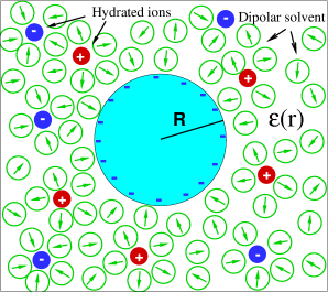
Figure 1: Schematic representation of a charged nanoparticle immersed in an electrolyte. Cations and anions are represented by solid red and blue balls, respectively. The surface charges are negative. Dipolar solvent molecules (empty green balls) near the surface are ordered under the influence of the strong electric field, leading to nonuniform dielectric permittivity.

Now we consider a special case of a charged nanoparticle with radius $R$ surrounded by an electrolyte (see Fig. 1). The surface charge is distributed uniformly on the surface with density $\sigma$ to make the potential field spherically symmetric. Thus, the potential field and ionic concentration densities are spherically symmetric in spherical coordinates $(r,\theta,\phi)$. We have the Neumann boundary condition for electric potential on the surface

$$-\varepsilon(r)\left.\frac{\partial\Phi}{\partial r}\right|_{r=R}=4\pi q\sigma.$$ (46)

Note here we have used the dimensionless surface charge density and $q=\ell_{B}/L$, and the dielectric permittivity is also dimensionless which is relative to the water dielectric permittivity. The origin of the sphere is set to be $r=0$ in the spherical coordinates. Clearly, we have the fact that the $i$th ion cannot penetrate the region $r<R+a_{i}$ due to the hard-wall repulsion to mobile ions. However, in order to maintain the continuous density profiles, we simplify this boundary effect for asymmetric electrolytes and assume the modified boundary is located at $r=R+a$ with $a=\max a_{i}$. Thus, the modified boundary condition is

$$-\varepsilon(r)\left.\frac{\partial\Phi}{\partial r}\right|_{r=R+a}=4\pi q\sigma\frac{R^{2}}{(R+a)^{2}}.$$ (47)

The far field conditions for electric potential is the decaying condition, $\Phi(r\rightarrow+\infty)=0$.

In this special spherical geometry, the dimensions in the self energy $u_{i}$ can be reduced, where $\widetilde{u}_{1}$ in Eq. (42) is simplified as,

$$\widetilde{u}_{1} =\frac{1}{\varepsilon}\lim_{\mathbf{r}^{\prime}\rightarrow\mathbf{r}}[\mathcal{H}^{(2)}(\mathbf{r},\mathbf{r}^{\prime})-\mathcal{H}_{0}(\mathbf{r},\mathbf{r}^{\prime})]$$ (48)

$$=-\frac{1}{2\varepsilon}\int v^{2}(r^{\prime\prime})\frac{e^{-v_{0}(r)\sqrt{{r^{\prime\prime}}^{2}+r-2rr^{\prime\prime}\cos\theta}}}{{r^{\prime\prime}}^{2}+r-2rr^{\prime\prime}\cos\theta}{r^{\prime\prime}}^{2}\sin\theta dr^{\prime\prime}d\theta$$

$$=-\frac{1}{2\varepsilon}\int_{0}^{+\infty}v^{2}(r^{\prime\prime})\frac{r^{\prime\prime}}{r}dr^{\prime\prime}\int^{v^{2}(r^{\prime\prime})|r+r^{\prime\prime}|}_{v^{2}(r^{\prime\prime})|r-r^{\prime\prime}|}\frac{e^{-z}}{z}dz.$$

The exponential integral is a special function and can be pre-computed. The computational cost of evaluating $\delta\mathcal{H}(\mathbf{r}\rightarrow\mathbf{r}^{\prime})$ for each point $\mathbf{r}^{\prime}$ becomes only a one-dimensional integral for $r^{\prime\prime}$.

We propose a self-consistent iterative algorithm to solve the SCF and SCF-L models. The algorithm is composed of two alternating steps: (1) For given $c_{i}^{(k)}$ and $\Phi^{(k)}$, we update $u_{i}^{(k)}$; and (2) for given $u_{i}^{(k)}$, we solve the modified PB equation for $\Phi^{(k+1)}$ subject to given boundary conditions. The iterative scheme for time steps is as follows,

$$u_{i}^{(k)}=\frac{\widetilde{u}_{1}^{(k)}}{1-\varepsilon^{(k)}\widetilde{u}_{1}^{(k)}a_{i}}+\frac{1}{a_{i}}\left[\frac{1}{\varepsilon^{(k)}}-\frac{1}{\varepsilon_{0}}\right],$$ (49)

$$\widetilde{u}_{1}^{(k)}=-\int\frac{[v^{(k)}(\mathbf{r}^{\prime\prime})]^{2}\exp[v^{(k)}(\mathbf{r})|\mathbf{r}-\mathbf{r}^{\prime\prime}|]}{4\pi\varepsilon^{(k)}(\mathbf{r})|\mathbf{r}-\mathbf{r}^{\prime\prime}|^{2}}d\mathbf{r}^{\prime\prime},$$ (50)

$$-2I_{0}\epsilon^{2}\nabla\cdot\varepsilon^{(k+1)}\nabla\Phi^{(k+1)}=\sum_{i}z_{i}c_{i0}e^{-U_{i}^{(k+1)}-S^{(k+1)}},$$

(51)

$$U_{i}^{(k+1)}=z_{i}\Phi^{(k+1)}+\frac{1}{2}z_{i}^{2}qu_{i}^{(k)},$$ (52)

$$S^{(k+1)}=\log\big{[}1+\sum_{j}\nu c_{j0}\big{(}e^{-U_{j}^{(k+1)}}-1\big{)}\big{]},$$ (53)

for $k=0,1,2,...,K$ and the iterative steps are performed until the convergence criteria $|u_{i}^{(k+1)}-u_{i}^{(k)}|<\delta$ is arrived, where $\delta$ is a small tolerant value. Here, we shall note that $\varepsilon$ and $v$ are functions of $\Phi$ and $c_{i}$. This numerical scheme follows a recent work Xu and Maggs (2014) for solvents of uniform dielectric function where the self-Green’s function in the DH equation can be efficiently solved by a method of the selected inversion. Differently, in this paper a numerical integration is used for the self energy, thus we can work on more general geometries.

The sub-level of the iterative scheme is embodied in the solution of the modified PB equation (51), which shows high nonlinearity. We could in general use the iterative scheme at the $(k)$th loop as

$$-2I_{0}\epsilon^{2}\nabla\cdot\varepsilon^{[l]}\nabla\Phi^{[l+1]}-\gamma^{[l]}\Phi^{[l+1]}=\sum_{i}z_{i}c_{i}^{[l]}-\gamma^{[l]}\Phi^{[l]},$$ (54)

where $c_{i}^{[l]}$ means the potential in $U_{i}$ and $S$ uses the value from the $l$th step, and the relaxation function $\gamma(\textbf{r})$ is defined as

$$\gamma(\textbf{r})=|\sum_{i}z_{i}c_{i}|/(|\Phi|+\delta_{0}),$$ (55)

with $\delta_{0}=10^{-8}$. Here we use the index $[\cdot]$ to represent the sub-iteration in the $(k)$th loop of the self-consistent iteration. This iteration stops when the convergence criteria $|\Phi^{[l+1]}-\Phi^{[l]}|<\delta$ is arrived.

For the physical setting with one macroion, the mean potential is spherically symmetric, hence the space discretization for Eq. (54) can be done by the central difference scheme for one-dimensional equation along the radial direction. The composite trapezoidal rule is used to approximate the integral in computing Eq. (48) for $\tilde{u}_{1}$.

We have not mentioned the direct numerical method for solving the self Green’s function. Solving the diagonal elements of lattice Green’s function from the generalized DH equation can be done by the use of selected inversion Lin et al. (2011a, b), which has been shown to reduce the computational cost a lot with point charge limit Xu and Maggs (2014); Xu et al. (2014). However, direct solvers of problems with inhomogeneous dielectric constant and size effect still remain challenging since it is a two-scale problem and we have to use a mesh size much smaller than an ion radius.

IV Results

In this section, we present numerical results for different systems of binary electrolytes surrounding a spherical macroion. We study the position-dependent dielectric constant $\varepsilon(\mathbf{r})$, compared with results from MC simulations. We then perform calculations for the SCF model with the field-dependent dielectric function. We use 1:1 and 2:1 salts, where anions are coions and always monovalent. Divalent counterions are used for strongly correlated systems, for which a correct treatment of electrostatic self energy is essential. Without specific statement, ions have radius of $a=0.225~{}\textup{nm}$, the simulations are performed at room temperature and the relative dielectric constant is $80$ for the bulk water, so the Bjerrum length $\ell_{B}=7.14~{}\textup{nm}$. The dimensional dipole moment is chosen as $p_{0}=4.8~{}\textup{D}$ (Abrashkin et al., 2007) for keeping the bulk water density $c_{d}=55~{}\textup{M}$. Surface charge density is varied within $0<-\sigma<3~{}\textup{e/nm}^{2}$, which describes most of the environments in biological or physical systems.

IV.1 Space-dependent dielectric function

In the following two groups of simulations, we consider simulated systems with given space-dependent dielectric functions. We take the radius of macroion as $R=2~{}\textup{nm}$, and the grid size for the SCF approximation as $3.75\times 10^{-3}~{}\textup{nm}.$

Electrolyte with 1:1 salts. We first consider that the macroion is surrounded by an electrolyte of $50~{}\textup{mM}$ 1:1 salts. A ramp shape of radial function is used to describe the dielectric permittivity, given by the following formula,

$$\varepsilon(r)=\varepsilon_{W}+\frac{\varepsilon_{C}-\varepsilon_{W}}{1+\exp[(r-2.45)/\lambda]},$$ (56)

where the unit for the spatial length is nm, and $\lambda=0.2~{}\textup{nm}$ is the length scale for the region of varying dielectric. We shall see the dielectric constant is $\varepsilon_{C}$ in the deep of the macroion, and $\varepsilon_{W}$ in the bulk water. Experimental measurements and computational studies have indicated that the dielectric permittivities of various ionic fluids near different interfaces can be fitted by the exponential function Teschke et al. (2001); Podgornik et al. (1987). We take $\varepsilon_{C}=10\varepsilon_{0}$ and $\varepsilon_{W}=80\varepsilon_{0}.$ In Fig. 2, the counterion and coion density distributions along the radial direction are plotted by numerically solving the SCF equations and particle-based MC simulations. Two sets of surface charge densities, $\sigma=-0.2$ and $-1.6~{}\textup{e/nm}^{2}$, are taken to check the accuracy of the SCF computation. To run the MC simulation, the harmonic interpolation method (HIM) Fahrenberger et al. (2014) is applied to calculate ion-ion pairwise energies with well treated boundary conditions for the Hamiltonian. The simulation volume is a concentric cell of radius $R_{c}=8.629~{}\textup{nm}$.

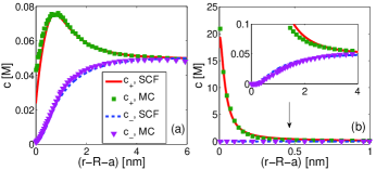
Figure 2: Counterion and coion concentration profiles as a function of the distance to the surface in 1:1 symmetric electrolytes with bulk concentration $c_{\pm}=50$ mM and surface charge $\sigma=-0.2~{}\textup{e/nm}^{2}$ (a) and $\sigma=-1.6~{}\textup{e/nm}^{2}$ (b). The ramp shape of dielectric profile is given by Eq. (56). Both SCF and MC simulations are presented.

For a surface of low surface charge, the electrostatic attraction between the macroion and counterions is weak, while the Born solvation energy increases when an ion approaches to the surface. It can be seen from 2(a) that the counterion is depleted near the surface, leading to an obvious nonmonotonic counterion concentration. For the strong surface charge, however, the attraction from the macroion dominates, clear depletion effect is not observed from 2(b). The SCF results in both weak and strong coupling cases are shown in good agreement with MC simulations.

Electrolyte with 2:1 salts. In the second group of systems, we consider a sharp jump of dielectric permittivity across the macroion surface with $\varepsilon_{C}=2\varepsilon_{0}$ and $\varepsilon_{W}=80\varepsilon_{0}$ inside and outside it, and an electrolyte of $50~{}\textup{mM}$ 2:1 salts which will show strong correlation effects for high surface charges. The dielectric-boundary effect is of interest in community Hatlo and Lue (2008); Messina (2009); Wang and Ma (2010); Gan et al. (2012); Jadhao et al. (2013); Wang and Wang (2013); Zwanikken and de la Cruz (2013). For example, the theoretical treatment of dielectric-boundary effects for both weak and strong coupling cases was also developed Bakhshandeh et al. (2011). It is then of interest to study the interplay between dielectric-boundary (image charge) and correlation effects in the SCF framework, verified with MC simulations. Two surface charge densities $\sigma=-0.2$ and $-2~{}\textup{e/nm}^{2}$ are taken. The radius of the simulation cell for MC calculations is $10~{}\textup{nm}$. For this setup, the image charge method Cai et al. (2007); Gan and Xu (2011) is used to obtain accurate MC results. As aforementioned, the Born series for the self energy has slow convergence for the sharp dielectric variation and Eq. (48) fails when it integrates over the whole domain. In order to make the Born series work, we take the lower limit of integral Eq. (48) as $R+a$ for $\widetilde{u}_{1}$, and follow similar technique for planar interfaces Xu et al. (2014) to introduce the dielectric effect from the macroion by a WKB type approximation using image charges for an updated self energy,

$$\widetilde{u}_{1}^{\prime}=\widetilde{u}_{1}+\sum_{\ell=1}^{L}\frac{z_{\ell}\exp(\widetilde{u}_{1}D_{\ell})}{\varepsilon_{W}D_{\ell}},$$ (57)

where index $\ell$ means the $\ell$th image charge, $z_{\ell}$ is its strength due to a unit source charge, and $D_{\ell}$ is its distance to the source charge; for these parameters see Eqs. (11)-(12) in Ref. Gan and Xu (2011). Both SCF and MC simulations use three image charges.

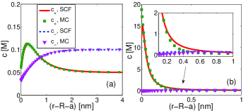
Figure 3: Counterion and coion concentration profiles as a function of the distance to the surface in 2:1 symmetry electrolytes with bulk concentration $c_{+}=50$ mM and surface charge $\sigma=-0.2~{}\textup{e/nm}^{2}$ (a) and $\sigma=-2~{}\textup{e/nm}^{2}$ (b). A sharp dielectric jump is across the colloidal surface. Both SCF and MC simulations are presented.

The results are presented in Fig. 3 for both weak and strong surface charge densities. From the left panel, we shall see that the WKB type approximation is very accurate for the dielectric effect, and the SCF and MC results are in a perfect agreement. For the weak-coupling system (Fig. 3(a)), the image charges repel mobile ions and a depletion zone is formed near the surface. For the strong-coupling system (Fig. 3(b)), they are screened by the surface charge since the image charges are dipole effects. The MC simulation does not predict a depletion zone, while the SCF result has a short interval for the depletion due to the steric effect applied to the double-layer ions in the vicinity of the surface. Both results show much higher counterion density near the surface than the bulk region with a factor of $\sim 300$ times ($15~{}\textup{M}$ vs. $50~{}\textup{mM}$). Both coion distribution profiles are slightly nonmonotonic, indicating a possibility of overscreening inside the double layer. These nonmonotonic curves are important signals for the correlation-induced charge inversion widely studied in literature Besteman et al. (2004); Pittler et al. (2006); Messina (2002); Tanaka (2003); Diehl and Levin (2006); Lenz and Holm (2008); Gan et al. (2012). The results shown in the two panels demonstrate that the SCF model can accurately capture the dielectric-boundary effect and the ion-ion electrostatic correlation.

IV.2 Field-dependent dielectric function

We have seen that the SCF theory can accurately capture the effects of electrostatic correlation, dielectric boundary and varying dielectric permittivity by a comparison with particle-base MC simulations with a fixed space-dependent dielectric function. In this section, we study equilibrium properties for systems of field-dependent dielectric function using the Langevin-SCF model. We consider both 1:1 and 2:1 salts with a fixed salt density $100~{}\textup{mM}$ and set the radius of the macroion, $R=4~{}\textup{nm}$. The dielectric-boundary effect is ignored by assuming the dielectric constant for $r<R+a$ is uniform and equal to $\varepsilon(R+a)$, which greatly improves the convergence of the Born series. For the numerical approximation, we take the grid size as $2.5\times 10^{-3}~{}\textup{nm}$.

IV.2.1 Effect of the ion correlation

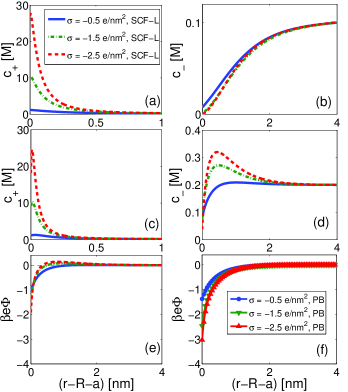
Figure 4: Ion concentrations and electric potentials for SCF calculations with field-dependent dielectric function (SCF-L). (a)(b) Ion concentrations for 1:1 salts; (c)(d) Ion concentrations for 2:1 concentration; (e)(f) Electric potential profiles for 2:1 salts by SCF-L and classical PB models.

In Fig. 4, numerical results of ionic concentrations and electric potentials for three different surface charges $\sigma=-0.5,-1.5$ and $-2.5~{}\textup{e/nm}^{2}$ are given. Correspondingly, the coupling parameters for 1:1 salts are $\Xi=1.6$, 4.8 and 8.0, and those for 2:1 salts are $\Xi=12.8$, 38.4 and 64.1. The upper and middle panels show the cation and anion density distributions, (a)(b) for 1:1 salts, and (c)(d) for 2:1 salts. The bottom panels, (e)(f), are the electric potentials for 2:1 salts from both the SCF-L and classical PB predictions.

For monovalent ions, since the electric field only slightly changes the nearby permittivity at the surface, the Born-energy repulsion to mobile ions is weak and not enough to overcome the electrostatic attraction from the macroion surface. On the other side, the electrostatic correlation between monovalent ions is weak too, and the entropic effect leads to a monotonic neutralization of the surface charge along the radial direction. Therefore, with the increase of the surface charge, both cation and anion densities of monovalent salts remain monotonic curves.

For divalent ions, the situations are different. The strength of electric field is high near the surface. This produces the decrement of the dielectric permittivity as an output. The Born solvation energy is repulsive and has a quadratic relation with the ion valence. Although the surface-charge attraction is strong, a depletion zone can be observed for high surface charge densities $\sigma=-1.5$ and $-2.5~{}\textup{e/nm}^{2}$, demonstrating that the zone is difficult to access by mobile ions due to the repulsion from the Born solvation energy. On the other hand, for these two surface densities, coion densities have a sharp increase up to a maximum at the one-ion-diameter distance, then decay to the bulk value monotonically. Observed from the distributions of electric potentials, the curves reverse the sign at the nearby distance, predicting a positive potential at the far field. This is the result of the correlation. Strange charge inversion phenomenon for multivalent counterions has been confirmed theoretically Shklovskii (1999); Quesada-Pérez et al. (2003); Diehl and Levin (2006) and experimentally by electrophoresis mobility Martin-Molina et al. (2003); Quesada-Pérez et al. (2005); Schneider et al. (2011). This clearly demonstrates again that the SCF model describes the electrostatic correlation. Ignoring the many-body correlation, the classical PB theory does not predict the charge inversion and as shown in Fig. 4(f) that the electric potentials are always negative with the increase of $\sigma$.

IV.2.2 Effects of the field-dependent permittivity

In Fig. 5(a)(b), the relative dielectric functions for 1:1 and 2:1 salts are illustrated in the cases of $\sigma=-0.5,~{}-1.5$ and $-2.5~{}\textup{e/nm}^{2}$. We shall see that the relative dielectric function is rapidly increased from $\sim 55$ to $>75$ for a distance less than one ion radius. In order to probe the effect of the dielectric variation in this small region, we present comparisons for the SCF calculations between using this field-dependent dielectric function and using uniform water dielectric constant $\varepsilon_{W}=80\varepsilon_{0}$. We call both results as the SCF-L and SCF, respectively.

Since the surface charge density plays an important role to provide different electric field and then affects the solvent structural details within the double layer Frydel and Oettel (2011), we calculate the surface potential as a function of the surface charge density and present the results in Fig 5(c)(d). The difference of surface potentials between two models becomes larger with the increase of $\sigma$, and significant differences appear in both 1:1 and 2:1 salts for large surface charges. For the 2:1 salt, the relative difference is already very high when $-\sigma$ is slightly bigger than $0.5~{}\textup{e}/\textup{nm}^{2}$ ($5\%$ for $\sigma=-1~{}\textup{e}/\textup{nm}^{2}$ and $14\%$ for $\sigma=-2~{}\textup{e}/\textup{nm}^{2}$). These results shall lead to the conclusion that the effect of field-dependent dielectric permittivity (i.e., the orientation of interfacial water molecules) are important for double-layer structure.

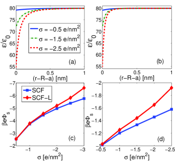
Figure 5: The relative dielectric profiles as functions of radial distance to the surface in (a) 1:1 and (b) 2:1 symmetric electrolytes at room temperature $\ell_{B}=0.714~{}\textup{nm}$ with three different surface charge densities. Comparison of surface potentials with SCF model (homogeneous water permittivity) and SCF-L model in: (c) 1:1 symmetric electrolyte and (d) 2:1 symmetric electrolyte.

IV.2.3 Effect of the ionic size

At last, let us see how the ionic size asymmetry affects the double-layer structure. We remain the anion radius of $a_{-}=0.225~{}\textup{nm}$, and consider two different cation (counterion) radii $a_{+}=0.225~{}\textup{nm}$ and $a_{+}=0.18~{}\textup{nm}$. The effect of ionic size is minor at the weak coupling regime. So we consider valence-symmetric electrolytes for the strong-coupling regime by setting the Bjerrum length $\ell_{B}=2.856~{}\textup{nm}$, a four times larger than the water Bjerrum length at room temperature. We can think this large Bjerrum length is because of a low temperature or a low bulk dielectric constant or multivalent ion species.

Fig. 6 plots the curves of both symmetric and asymmetric cases with three surface charge densities $\sigma=-0.2,-0.3$ and $-0.4~{}\textup{e}/\textup{nm}^{2}$. We shall note that for a large $\ell_{B}$, the electrostatic correlations between ions are strong and thus the nonmonotonic concentration should be predicted when $\sigma$ is not very low. On the other hand, the smaller counterion radius greatly increases the correlation self energy which is negative and thus is favorable for the ion congregation in the double layer. Both counterion and coion nearby densities of the asymmetric case (smaller counterions) are higher than the symmetric case, and this effect is enlarged with the increase of the surface charge density, as is shown in the insets. Fig. 6(d) shows the electric potentials in the case of $\sigma=-0.4~{}\textup{e}/\textup{nm}^{2}$ for symmetric and asymmetric ionic sizes. The coupling parameter is $\Xi=20.50$. We observed the charge inversion for the asymmetric case other from the symmetric case, illustrating the ionic sizes are very much relevant to ion correlations.

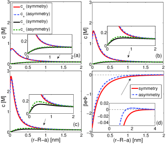
Figure 6: Ion concentration and potential profiles for electrolytes of 1:1 salts with $\ell_{B}=2.856~{}\textup{nm}$. Symmetric size ($a_{+}=a_{-}=0.225~{}\textup{nm}$) and asymmetric sizes ($a_{+}=0.18~{}\textup{nm},a_{-}=0.225~{}\textup{nm}$). Ion concentrations for: (a) $\sigma=-0.2~{}\textup{e}/\textup{nm}^{2}$; (b) $\sigma=-0.3~{}\textup{e}/\textup{nm}^{2}$; and (c) $\sigma=-0.4~{}\textup{e}/\textup{nm}^{2}$. (d) The electric potentials for $\sigma=-0.4~{}\textup{e}/\textup{nm}^{2}$.

V Conclusions

We have introduced a modified version of the self-consistent field model for electrostatic interaction, and developed a hybrid numerical method for the numerical solution of the resulted system of PDEs. In particular, we proposed a new and efficient way to deal with the solution of self Green’s function for a test ion as a charged hard sphere in a dielectrically inhomogeneous medium. As a result, the expensive direct numerical implementation for a multiscale (macroion and small ions) and high-dimensional Green’s function problem (i.e., 6D problem for a 3D geometry) is avoided.

The numerical results are shown to capture many-body effects, such as the effect of inhomogeneous dielectric permittivity (the Born energy), size effect and ionic correlations. These effects are thought to be significant in many biological and physical phenomena near aqueous electrolyte interfaces. Strong ionic correlations lead to the charge inversion which has also been well reproduced by the SCF model. The numerical results are shown to quantitatively match the results from MC simulations. We shall notice the drawback of the approximation with Born series is obvious for irregular surfaces and remain the challenges of overcoming this issue by developing fast and accurate numerical methods as our future work. The effect of correlation to charge dynamics shall be an important direction to be addressed in the future, which will be studied in the framework of modified Poisson-Nernst-Planck equations.

References

- Levin (2002) Y. Levin, Rep. Prog. Phys. 65, 1577 (2002).
- Hunter (1981) R. J. Hunter, Zeta Potential in Colloidal Sciences: Principles and Applications (Academic, Lundon, 1981).
- Joly et al. (2004) L. Joly, C. Ybert, E. Trizac, and L. Bocquet, Phys. Rev. Lett. 93, 257805 (2004).
- French et al. (2010) R. H. French, V. A. Parsegian, R. Podgornik, R. F. Rajter, A. Jagota, J. Luo, D. Asthagiri, M. K. Chaudhury, Y.-M. Chiang, S. Granick, et al., Rev. Mod. Phys. 82, 1887 (2010).
- Walker et al. (2011) D. A. Walker, B. Kowalczyk, M. O. de la Cruz, and B. A. Grzybowski, Nanoscale 3, 1316 (2011).
- Besteman et al. (2004) K. Besteman, M. A. G. Zevenbergen, H. A. Heering, and S. G. Lemay, Phys. Rev. Lett. 93, 170802 (2004).
- Pittler et al. (2006) J. Pittler, W. Bu, D. Vaknin, A. Travesset, D. J. McGillivray, and M. Lösche, Phys. Rev. Lett. 97, 046102 (2006).
- Lozada-Cassou et al. (1982) M. Lozada-Cassou, R. Saavedra-Barrera, and D. Henderson, J. Chem. Phys. 77, 5150 (1982).
- Deserno et al. (2001) M. Deserno, F. Jiménez-Ángeles, C. Holm, and M. Lozada-Cassou, J. Phys. Chem. B 105, 10983 (2001).
- Grosberg et al. (2002) A. Y. Grosberg, T. T. Nguyen, and B. I. Shklovskii, Rev. Mod. Phys. 74, 329 (2002).
- Larsen and Grier (1997) A. E. Larsen and D. G. Grier, Nature 385, 230 (1997).
- Angelini et al. (2003) T. E. Angelini, H. Liang, W. Wriggers, and G. C. L. Wong, Proc. Nat. Acad. Sci. USA 100, 8634 (2003).
- Eisenberg (2011) B. Eisenberg, Adv. Chem. Phys. 31, 117 (2011).
- Fedorov and Kornyshev (2014) M. V. Fedorov and A. A. Kornyshev, Chem. Rev. 114, 2978 (2014).
- Boroudjerdi et al. (2005) H. Boroudjerdi, Y.-W. Kim, A. Naji, R. R. Netz, X. Schlagberger, and A. Serr, Phys. Rep. 416, 129 (2005).
- Borukhov et al. (1997) I. Borukhov, D. Andelman, and H. Orland, Phys. Rev. Lett. 79, 435 (1997).
- Kilic et al. (2007) M. S. Kilic, M. Z. Bazant, and A. Ajdari, Phys. Rev. E 75, 021503 (2007).
- Corry et al. (2003) B. Corry, S. Kuyucak, and S.-H. Chung, Biophys. J. 84, 3594 (2003).
- Graf et al. (2004) P. Graf, M. G. Kurnikova, R. D. Coalson, and A. Nitzan, J. Phys. Chem. B 108, 2006 (2004).
- Eisenberg et al. (2010) B. Eisenberg, Y. Hyon, and C. Liu, J. Chem. Phys. 133, 104104 (2010).
- Hansen and McDonald (2006) J. P. Hansen and I. R. McDonald, Theory of simple liquids (Academic Press, Amsterdam, 2006).
- Bazant et al. (2011) M. Z. Bazant, B. D. Storey, and A. A. Kornyshev, Phys. Rev. Lett. 106, 046102 (2011).
- Liu and Eisenberg (2013) J.-L. Liu and B. Eisenberg, J. Phys. Chem. B 117, 12051 (2013).
- Linse (2005) P. Linse, Adv. Polym. Sci. 185, 111 (2005).
- Messina (2009) R. Messina, J. Phys. Condens. Matter 21, 113102 (2009).
- Hasted et al. (1948) J. Hasted, D. Ritson, and C. Collie, J. Chem. Phys. 16, 1 (1948).
- Booth (1951) F. Booth, J. Chem. Phys. 19, 391 (1951).
- Booth (1955) F. Booth, J. Chem. Phys. 23, 453 (1955).
- Yeh and Berkowitz (1999) I.-C. Yeh and M. L. Berkowitz, J. Chem. Phys. 110, 7935 (1999).
- Fulton (2009) R. L. Fulton, J. Chem. Phys. 130, 204503 (2009).
- Gur et al. (1978) Y. Gur, I. Ravina, and A. J. Babchin, J. Colloid Interf. Sci. 64, 333 (1978).
- Paunov et al. (1996) V. Paunov, R. Dimova, P. Kralchevsky, G. Broze, and A. Mehreteab, J. Colloid Interf. Sci. 182, 239 (1996).
- Ben-Yaakov et al. (2011) D. Ben-Yaakov, D. Andelman, and R. Podgornik, J. Chem. Phys. 134, 074705 (2011).
- Wang et al. (2011) H. Wang, J. Varghese, and L. Pilon, Electrochimica Acta 56, 6189 (2011).
- Frydel and Oettel (2011) D. Frydel and M. Oettel, Phys. Chem. Chem. Phys. 13, 4109 (2011).
- Bonthuis et al. (2011) D. J. Bonthuis, S. Gekle, and R. R. Netz, Phys. Rev. Lett. 107, 166102 (2011).
- Bonthuis et al. (2012) D. J. Bonthuis, S. Gekle, and R. R. Netz, Langmuir 28, 7679 (2012).
- Bonthuis and Netz (2013) D. J. Bonthuis and R. R. Netz, J. Phys. Chem. B 117, 11397 (2013).
- Onsager and Samaras (1934) L. Onsager and N. N. T. Samaras, J. Chem. Phys. 2, 528 (1934).
- Podgornik (1989) R. Podgornik, J. Chem. Phys. 91, 5840 (1989).
- Netz and Orland (2000) R. R. Netz and H. Orland, Eur. Phys. J. E 1, 203 (2000).
- Netz and Orland (2003) R. R. Netz and H. Orland, Eur. Phys. J. E 11, 301 (2003).
- Wang (2010) Z. G. Wang, Phys. Rev. E 81, 021501 (2010).
- Wang and Wang (2013) R. Wang and Z.-G. Wang, J. Chem. Phys. 139, 124702 (2013).
- Lu and Xing (2014) B.-S. Lu and X. Xing, Phys. Rev. E 89, 032305 (2014).
- Buyukdagli et al. (2012) S. Buyukdagli, C. V. Achim, and T. Ala-Nissila, J. Chem. Phys. 137, 104902 (2012).
- Lau et al. (2002) A. W. C. Lau, D. B. Lukatsky, P. Pincus, and S. A. Safran, Phys. Rev. E 65, 051502 (2002).
- Born (1920) M. Born, Z. Phys. 1, 45 (1920).
- Xu and Maggs (2014) Z. Xu and A. Maggs, J. Comput. Phys. 275, 310 (2014).
- Luo et al. (2006) G. Luo, S. Malkova, J. Yoon, D. G. Schultz, B. Lin, M. Meron, I. Benjamin, P. Vanýsek, and M. L. Schlossman, Science 311, 216 (2006).
- Gillespie (2014) D. Gillespie, Microfluidics and Nanofluidics pp. 1–22 (2014).
- Li (2009) B. Li, Nonlinearity 22, 811 (2009).
- Li et al. (2013) B. Li, P. Liu, Z. Xu, and S. Zhou, Nonlinearity 26, 2899 (2013).
- Frydel and Levin (2012) D. Frydel and Y. Levin, J. Chem. Phys. 137, 164703 (2012).
- Rosenfeld (1989) Y. Rosenfeld, Phys. Rev. Lett. 63, 980 (1989).
- Xu et al. (2014) Z. Xu, M. Ma, and P. Liu, Phys. Rev. E 90, 013307 (2014).
- Levin et al. (2009) Y. Levin, A. P. Dos Santos, and A. Diehl, Phys. Rev. Lett. 103, 257802 (2009).
- Levin (2009) Y. Levin, Phys. Rev. Lett. 102, 147803 (2009).
- Wang and Wang (2014) R. Wang and Z.-G. Wang, Phys. Rev. Lett. 112, 136101 (2014).
- Abrashkin et al. (2007) A. Abrashkin, D. Andelman, and H. Orland, Phys. Rev. Lett. 99, 077801 (2007).
- Frydel (2014) D. Frydel, Personal Communication (2014).
- Bockris and Reddy (1998) J. Bockris and A. Reddy, Modern Electrochemistry (Plenum Press, New York, 1998).
- Kalcher and Dzubiella (2009) I. Kalcher and J. Dzubiella, J. Chem. Phys. 130, 134507 (2009).
- Li et al. (2014) B. Li, J. Wen, and S. Zhou, Personal Communication (2014).
- Renou et al. (2014) R. Renou, M. Ding, H. Zhu, A. Szymczyk, P. Malfreyt, and A. Ghoufi, J. Phys. Chem. B 118, 3931 (2014).
- Frydel (2011) D. Frydel, J. Chem. Phys. 134, 234704 (2011).
- Lin et al. (2011a) L. Lin, C. Yang, J. Lu, L. Ying, and W. E, SIAM J. Sci. Comput. 33, 1329 (2011a).
- Lin et al. (2011b) L. Lin, C. Yang, J. C. Meza, J. Lu, L. Ying, and W. E, ACM Trans. Math. Softw. 37, 40:1 (2011b).
- Teschke et al. (2001) O. Teschke, G. Ceotto, and E. De Souza, Phys. Rev. E 64, 011605 (2001).
- Podgornik et al. (1987) R. Podgornik, G. Cevc, and B. Žekš, J. Chem. Phys. 87, 5957 (1987).
- Fahrenberger et al. (2014) F. Fahrenberger, Z. Xu, and C. Holm, J. Chem. Phys. 141, 064902 (2014).
- Hatlo and Lue (2008) M. M. Hatlo and L. Lue, Soft Matter 4, 1582 (2008).
- Wang and Ma (2010) Z. Y. Wang and Y. Q. Ma, J. Phys. Chem. B 114, 13386 (2010).
- Gan et al. (2012) Z. Gan, X. Xing, and Z. Xu, J. Chem. Phys. 137, 034708 (2012).
- Jadhao et al. (2013) V. Jadhao, F. J. Solis, and M. O. de la Cruz, J. Chem. Phys. 138, 054119 (2013).
- Zwanikken and de la Cruz (2013) J. W. Zwanikken and M. O. de la Cruz, Proc. Nat. Acad. Sci. USA 110, 5301 (2013).
- Bakhshandeh et al. (2011) A. Bakhshandeh, A. P. dos Santos, and Y. Levin, Phys. Rev. Lett. 107, 107801 (2011).
- Cai et al. (2007) W. Cai, S. Deng, and D. Jacobs, J. Comput. Phys. 223, 846 (2007).
- Gan and Xu (2011) Z. Gan and Z. Xu, Phys. Rev. E 84, 016705 (2011).
- Messina (2002) R. Messina, J. Chem. Phys. 117, 11062 (2002).
- Tanaka (2003) M. Tanaka, Phys. Rev. E 68, 061501 (2003).
- Diehl and Levin (2006) A. Diehl and Y. Levin, J. Chem. Phys. 125, 054902 (2006).
- Lenz and Holm (2008) O. Lenz and C. Holm, Eur. Phys. J. E. 26, 191 (2008).
- Shklovskii (1999) B. I. Shklovskii, Phys. Rev. E 60, 5802 (1999).
- Quesada-Pérez et al. (2003) M. Quesada-Pérez, E. González-Tovar, A. Martín-Molina, M. Lozada-Cassou, and R. Hidalgo-Álvarez, Chem. Phys. Chem. 4, 234 (2003).
- Martin-Molina et al. (2003) A. Martin-Molina, M. Quesada-Pérez, F. Galisteo-González, and R. Hidalgo-Alvarez, J. Phys. Condens. Matter 15, S3475 (2003).
- Quesada-Pérez et al. (2005) M. Quesada-Pérez, E. González-Tovar, A. Martín-Molina, M. Lozada-Cassou, and R. Hidalgo-Álvarez, Colloids and Surfaces A: Physicochemical and Engineering Aspects 267, 24 (2005).
- Schneider et al. (2011) C. Schneider, M. Hanisch, B. Wedel, A. Jusufi, and M. Ballauff, J. Colloid Interf. Sci. 358, 62 (2011).