Cosmological three-coupled scalar theory for the dS/LCFT correspondence

Abstract

We investigate cosmological perturbations generated during de Sitter inflation in the three-coupled scalar theory. This theory is composed of three coupled scalars ($\phi_{p},p=1,2,3$) to give a sixth-order derivative scalar theory for $\phi_{3}$, in addition to tensor. Recovering the power spectra between scalars from the LCFT correlators in momentum space indicates that the de Sitter/logarithmic conformal field theory (dS/LCFT) correspondence works in the superhorizon limit. We use LCFT correlators derived from the dS/LCFT differentiate dictionary to compare cosmological correlators (power spectra) and find also LCFT correlators by making use of extrapolate dictionary. This is because the former approach is more conventional than the latter. A bulk version dual to the truncation process to find a unitary CFT in the LCFT corresponds to selecting a physical field $\phi_{2}$ with positive norm propagating on the dS spacetime.

1 Introduction

The Lee-Wick (LW) model of a fourth-order derivative scalar theory with $\hat{\phi}$ has provided a cosmological bounce which could avoid the big bang singularity [1]. By introducing an auxiliary field (LW scalar $\tilde{\phi}$) and redefining the normal scalar field as $\phi=\hat{\phi}+\tilde{\phi}$, the fourth-order Lagrangian can be expressed in terms of two second-order Lagrangians where the kinetic and mass terms of the LW scalar have the opposite sign compared the signs for the normal scalar. The LW scalar plays the role of a ghost scalar and thus, it is responsible for giving a bouncing solution. In the contracting phase, $\phi$ dominates while $\phi$ freezes and $\tilde{\phi}$ still oscillates near the bounce. In the expanding phase, $\phi$ dominates again. Vacuum fluctuations in the contracting phase have led to a scale-invariant spectrum of cosmological perturbations. Recently, it was proposed that the bounce inflation scenario can simultaneously explain the Planck and BICEP2 observations better than the $\Lambda$CDM model [2].

On the other hand, the singleton theory [3] was used widely to derive the anti de Sitter (AdS)/logarithmic conformal field theory (LCFT) correspondence [4, 5, 6, 7] as well as the dS/LCFT correspondence [8, 9]. The singleton is a bulk Lagrangian composed of dipole fields ($\phi_{1},\phi_{2}$) to give a fourth-order differential equation $(\nabla^{2}-m^{2})^{2}\phi_{2}=0$ for $\phi_{2}$ [equivalently, a second-order coupled equation $(\nabla^{2}-m^{2})\phi_{2}=\mu^{2}\phi_{1}$] on the AdS/dS background, even though its starting Lagrangian is second-order. The field $\phi_{1}$ can be seen as an auxiliary field to lower the number of derivatives in the fourth-order Lagrangian. The similarity between the LW model and singleton theory is the connection of ($\phi\leftrightarrow\phi_{1},\hat{\phi}\leftrightarrow\phi_{2}$) and a difference is the absence of the LW scalar $\tilde{\phi}$ in the singleton theory. Also, the LW model has two different masses, but the singleton has the same mass. Here we are interested in studying the singleton in the AdS/dS background induced by the negative/positive cosmological constants. To that end, the singleton was used to derive the LCFT [10, 11] on the boundary of AdS/dS which induces a non-unitraity problem. The singleton was of interest from the cosmological point of view for two reasons: The power spectrum during dS inflation is not scale-invariant even in the limit of zero-mass because of the presence of $(H/2\pi)^{2}\ln[\epsilon k]$ in the superhorizon and it provides one example in which the Suyama-Yamaguchi inequality is reversed [8]. This inequality describes the connection between the collapsed limit of four-point correlator and the squeezed limit of three-point correlator [12].

In order to resolve the non-unitarity problem confronted in the singleton, one has to truncate log-modes out by imposing the appropriate AdS boundary conditions [13]. A rank of the LCFT refers to the dimensionality of the Jordan cell. The rank-2 LCFT dual to a critical gravity has a rank-2 Jordan cell and thus, an operator has a logarithmic (log) partner. Stating simply, a log partner is dual to $\phi_{2}$ whose equation is a fourth-order equation. However, there remains nothing for the rank-2 LCFT after making truncation. This implies that there is no power spectrum. The LCFT dual to a tricritical gravity has a rank-3 Jordan cell [14] and an operator has two log partners of log and log². After truncation, there remains a unitary subspace with non-negative state. For simplicity, it is natural to consider a sixth-order scalar field theory to cast off the non-unitarity problem. In order to avoid a difficulty in dealing with a single sixth-order theory, we introduce an equivalent three-coupled scalar fields ($\phi_{1},\phi_{2},\phi_{3}$) with degenerate masses $m^{2}$ [15, 16]. A bulk version dual to the truncation process to find a unitary CFT in the rank-3 LCFT corresponds to selecting a physical field $\phi_{2}$ with positive norm propagating on the dS spacetime. After truncation, the only non-zero power spectrum will be ${\cal P}_{22,0}=\xi^{2}(\epsilon k)^{2w}$ which is surly non-negative.

At this stage, we would like to mention that this three-coupled scalar theory might be considered as a toy model of the tricritical gravity. However, it was pointed out that these linearized approaches of tricritical gravities have pathologies when considering the non-linear level [17]. This implies that calculations on the linearized level seemed to lend support to the possibility of truncating the theory. In this sense, we have to regard our model of the three-coupled scalar as a toy model of (linearized) tricritical gravities.

The canonical quantization of three-coupled scalar theory was performed with nontrivial commutation relations on the Minkowski spacetime. These commutation relations will be used to compute the power spectra of scalars when one chooses the Bunch-Davies (BD) vacuum in the subhorizon limit of dS inflation. This is considered as the dS/quantum field theory (QFT) correspondence in the subhorizon limit.

A single scalar field (inflaton) with a canonical kinetic term is generally known to be a promising model for describing the slow-roll (dS-like) inflation [18, 19]. Importantly, a recent detection of B-mode polarization has enhanced the occurrence of inflation at the GUT scale [20]. Also, it is worth noting that the dS/CFT correspondence [21] has firstly provided the derivation of the non-Gaussianity from the single field inflation in the superhorizon limit. [22]. If one accepts holographic inflation such that the dS inflation era of our universe is described by a dual CFT living on the slice ($\mathbb{R}^{3}$) at the end of inflation, the BICEP2 results might determine the central charge of the CFT [23].

Accordingly, it is promising to compute the power spectrum of the three-coupled scalar field theory generated during dS inflation because this theory provides non-canonical fourth-order and sixth-order equations, in addition to the canonical second-order equation. In order to compute the power spectrum, one needs to choose the BD vacuum in the subhorizon limit of $z\to\infty$ (UV region). Here, one has to quantize the three-coupled scalar fields canonically in the subhorizon limit whose commutation relations (5.7) are important to compute the power spectrum. This may provide a hint for the dS/QFT correspondence in the subhorizon region of $z\to\infty$ (UV region). Also, it is meaningful to check whether the dS/LCFT correspondence plays a crucial role in computing the power spectrum in the superhorizon limit of $z\to 0$ (IR region) [8]. We will observe that the commutation relations (5.7) between three scalars have the similar form as LCFT correlators (3.13), which shows the double correspondences of dS/QFT and dS/LCFT on the UV and IR regions, respectively.

2 Three-coupled scalar field theory

We consider the three-coupled scalar field theory where three fields ($\phi_{1},\phi_{2},\phi_{3}$) are coupled minimally to Einstein gravity as [13, 16, 24]

$$S=S_{\rm E}+S_{\rm TCS}$$ (2.1)

$$S_{\rm E}=\int d^{4}x\sqrt{-g}\Big{(}\frac{R}{2\kappa}-\Lambda\Big{)},$$ (2.2)

$$S_{\rm TCS}=-\int d^{4}x\sqrt{-g}\Big{[}\partial_{\mu}\phi_{1}\partial^{\mu}\phi_{3}+\frac{1}{2}\partial_{\mu}\phi_{2}\partial^{\mu}\phi_{2}+\mu^{2}\phi_{1}\phi_{2}+m^{2}\phi_{1}\phi_{3}+\frac{1}{2}m^{2}\phi^{2}_{2}\Big{]},$$ (2.3)

where $S_{\rm E}$ is introduced to provide de Sitter background with $\Lambda>0$ and $S_{\rm TCS}$ represents the three-coupled scalar theory. Here we have $\kappa=8\pi G=1/M^{2}_{\rm P}$, $M_{\rm P}$ being the reduced Planck mass, $m^{2}$ is the degenerate mass-squared, and $\mu^{2}$ is a parameter. We follow the conventions in [19] to compute the power spectrum.

The Einstein equation is given by

$$G_{\mu\nu}+\kappa\Lambda g_{\mu\nu}=2\kappa T_{\mu\nu}$$ (2.4)

with the energy-momentum tensor

$$T_{\mu\nu} = \partial_{\mu}\phi_{1}\partial_{\nu}\phi_{3}+\frac{1}{2}\partial_{\mu}\phi_{2}\partial_{\nu}\phi_{2}$$

$$\hskip 20.00003pt-\frac{1}{2}g_{\mu\nu}\Big{(}\partial_{\rho}\phi_{1}\partial^{\rho}\phi_{3}+\frac{1}{2}(\partial_{\rho}\phi_{2})^{2}+\mu^{2}\phi_{1}\phi_{2}+m^{2}\phi_{1}\phi_{3}+\frac{1}{2}m^{2}\phi_{2}^{2}\Big{)}.$$

Three scalar equations are obtained when one varies the action (2.3) with respect to $\phi_{3},\phi_{2},\phi_{1}$, respectively,

$$(\nabla^{2}-m^{2})\phi_{1}=0,~{}~{}(\nabla^{2}-m^{2})\phi_{2}=\mu^{2}\phi_{1},~{}~{}(\nabla^{2}-m^{2})\phi_{3}=\mu^{2}\phi_{2}$$ (2.5)

which are arranged to give degenerate fourth-order and sixth-order equations

$$(\nabla^{2}-m^{2})^{2}\phi_{2}=0,~{}~{}(\nabla^{2}-m^{2})^{3}\phi_{3}=0.$$ (2.6)

It shows how a higher-derivative scalar theory comes out from the second-order coupled action (2.3). This is so because of the presence of $\mu^{2}\phi_{1}\phi_{2}$-term in (2.3). We have always the same second-order equation $(\nabla^{2}-m^{2})\phi_{p}=0$ for $p=1,2,3$ without it.

When one chooses the vanishing scalars, the dS spacetime solution is given by

$$\bar{\phi}_{1}=\bar{\phi}_{2}=\bar{\phi}_{3}=0\to\bar{R}=4\kappa\Lambda.$$ (2.7)

Curvature quantities are given by

$$\bar{R}_{\mu\nu\rho\sigma}=H^{2}(\bar{g}_{\mu\rho}\bar{g}_{\nu\sigma}-\bar{g}_{\mu\sigma}\bar{g}_{\nu\rho}),~{}~{}\bar{R}_{\mu\nu}=3H^{2}\bar{g}_{\mu\nu}$$ (2.8)

with a constant Hubble parameter $H^{2}=\kappa\Lambda/3$. We represent the dS spacetime explicitly by choosing a conformal time $\eta$ as a flat slicing

$$ds^{2}_{\rm dS}=\bar{g}_{\mu\nu}dx^{\mu}dx^{\nu}=a(\eta)^{2}\Big{[}-d\eta^{2}+d{\bf x}\cdot d{\bf x}\Big{]}$$ (2.9)

with the conformal scale factor

$$a(\eta)=-\frac{1}{H\eta}\to a(t)=e^{Ht},$$ (2.10)

where the latter represents the scale factor for cosmic time $t$. During the dS stage, the scale factor $a$ goes from small to a very large value like $a_{f}/a_{i}\simeq 10^{30}$. It implies that the conformal time $\eta=-(aH)^{-1}$ runs from $-\infty$ (infinite past) to $0^{-}$ (infinite future). As is shown in Fig. 1, the UV/IR boundaries (${\rm\partial dS}_{\infty/0}$) of dS space are located at $\eta=-\infty$ and $\eta=0^{-}$, respectively, which make the boundary compact [21]. Also we recall that this coordinate system covers only half of dS space and thus, $\eta=-\infty$ corresponds to the past horizon. We emphasize that the BD vacuum must be chosen at $\eta=-\infty$, while the dual LCFT can be thought of as living on the slice ($\mathbb{R}^{3}$) at $\eta=-\epsilon(0<\epsilon\ll 1)$. This indicates that one has to take into account both boundaries of $\eta=-\infty$ and $-\epsilon$ to compute the power spectrum. This might imply the dS/QFT and dS/LCFT correspondences.

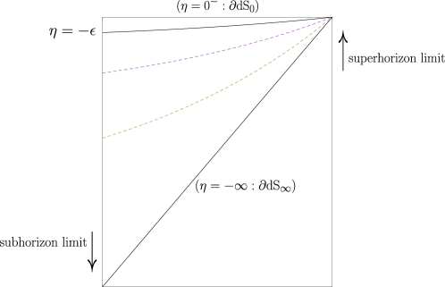
Figure 1: Penrose diagram of de Sitter inflation with the UV/IR boundaries (${\rm\partial dS}_{\infty/0}$) located at $\eta=-\infty$ and $\eta=0^{-}$. A slice ($\mathbb{R}^{3}$) at $\eta=-\epsilon$ is employed to define the LCFT. Conformal invariance in $\mathbb{R}^{3}$ at $\eta=-\epsilon$ is connected to the isometry group SO(1,4) of dS space. The dS isometry group acts as conformal group when fluctuations are superhorizon. Hence, correlators are expected to be constrained by conformal invariance. On the other hand, one introduces the BD vacuum in the subhorizon limit of $\eta\to-\infty$ to compute the power spectra.

For simplicity, we take the Newtonian gauge of $B=E=0$ and $\bar{E}_{i}=0$ for metric perturbation $h_{\mu\nu}$ around the dS background $\bar{g}_{\mu\nu}$ (2.9). Then, the perturbed metric is given by

$$ds^{2}=a(\eta)^{2}\Big{[}-(1+2\Psi)d\eta^{2}+2\Psi_{i}d\eta dx^{i}+\Big{\{}(1+2\Phi)\delta_{ij}+h_{ij}\Big{\}}dx^{i}dx^{j}\Big{]}$$ (2.11)

with transverse-traceless tensor $\partial_{i}h^{ij}=h=0$. Also, one has three scalar perturbations

$$\phi_{p}=\bar{\phi}_{p}+\varphi_{p},~{}~{}p=1,2,3.$$ (2.12)

In order to obtain the cosmological perturbed equations, one has to linearize the Einstein equation (2.4) directly around the dS spacetime, arriving at

$$\delta R_{\mu\nu}(h)-3H^{2}h_{\mu\nu}=0\to\bar{\nabla}^{2}h_{ij}=0.$$ (2.13)

Two scalars $\Psi$ and $\Phi$ are not physically propagating modes. $\Psi=-\Phi$ was found [19] when using the linearized Einstein equation, and it was used to define the comoving curvature perturbation in the slow-roll inflation. Also, a vector $\Psi_{i}$ is nonpropagating mode since it has no kinetic term. In the dS inflation, there is no coupling between $\{\Psi,\Phi\}$ and $\{\varphi_{p}\}$ because of vanishing background $\bar{\phi}_{p}=0$. The linearized scalar equations are given by

$$(\bar{\nabla}^{2}-m^{2})\varphi_{1}=0,$$ (2.14)

$$(\bar{\nabla}^{2}-m^{2})\varphi_{2}=\mu^{2}\varphi_{1},$$ (2.15)

$$(\bar{\nabla}^{2}-m^{2})\varphi_{3}=\mu^{2}\varphi_{2}.$$ (2.16)

These are combined to give a degenerate fourth-order equation and and a sixth-order equation

$$(\bar{\nabla}^{2}-m^{2})^{2}\varphi_{2}=0,$$ (2.17)

$$(\bar{\nabla}^{2}-m^{2})^{3}\varphi_{3}=0,$$ (2.18)

which are our main equations to be solved for cosmological purpose because a complete solution to a second-order equation (2.14) was given by the Hankel function.

3 dS/LCFT correspondence

Conformal invariance on the slice ($\mathbb{R}^{3}$) near $\eta=0^{-}$ is connected to the isometry group SO(1,4) of dS spacetime. The dS isometry group acts as conformal group when fluctuations are in the superhorizon limit of $\eta\to 0^{-}$. The two-point functions (correlators) are expected to be constrained by conformal invariance. For definiteness, we first consider the slice ($\mathbb{R}^{3}$) and its momentum space at $\eta=-\epsilon$ and then, take the limit of $\epsilon\to 0$ [8].

To derive the dS/LCFT correspondence, we first solve Eqs. (2.14), (2.17), and (2.18) in the superhorizon limit of $\eta\to 0^{-}$. Their solutions are given by

$$\varphi_{1,\eta\to 0}(\eta)\sim(-\eta)^{w},~{}~{}\varphi_{2,\eta\to 0}(\eta)\sim(-\eta)^{w}\ln[-\eta],~{}~{}\varphi_{3,\eta\to 0}(\eta)\sim(-\eta)^{w}\ln^{2}[-\eta]$$ (3.1)

with

$$w=\frac{3}{2}\Bigg{(}1-\sqrt{1-\frac{4m^{2}}{9H^{2}}}\Bigg{)}.$$ (3.2)

In the dS/CFT picture, the complementary series of $0<\frac{4m^{2}}{9H^{2}}<1$ have a dual interpretation in terms of a unitary CFT while the principal series of $\frac{4m^{2}}{9H^{2}}>1$ require a nonunitary CFT [25]. Hence, we choose the complementary series for developing the dS/LCFT correspondence. These solutions all satisfy the Dirichlet boundary condition of $\lim_{\eta\to 0^{-}}[\varphi_{p,0}]\to 0$.

Deriving cosmological correlator of a massive scalar from the dS/CFT dictionary, it is very important to note the following two statements [26]:
(i) In Lorentzian dS₄, the extrapolated bulk correlators are a sum of two contributions. One is the leading behavior of a CFT correlator of an operator with conformal dimension $w=\frac{3}{2}-\sqrt{\frac{9}{4}-\frac{m^{2}}{H^{2}}}$, while the other comes from the leading behavior of a CFT correlator of an operator with dimension $\triangle_{+}=\frac{3}{2}+\sqrt{\frac{9}{4}-\frac{m^{2}}{H^{2}}}$.
(ii) In Lorentzian dS₄, functional derivatives of late-time Schrödinger wavefunction produce CFT correlators with dimension $\triangle_{+}$ only.
The dominant term in (i) was computed by Witten for a particular scalar [27], whereas a massless version of statement (ii) was firstly made by Maldacena [21]. This indicates that the dS/CFT “extrapolate” and “differentiate” dictionaries are inequivalent to each other, while the AdS/CFT “extrapolate” and “differentiate” dictionaries are equivalent. Following (ii) to compute cosmological correlator of a massive scalar, it is inversely proportional to CFT correlator with dimension $\triangle_{+}$ as

$$\langle\phi(k)\phi(-k)\rangle\propto\frac{1}{\langle{\cal O}(k){\cal O}(-k)\rangle}\propto\frac{1}{k^{-3+2\triangle_{+}}}=k^{2w-3},$$ (3.3)

which leads to the power spectrum for a massive scalar in the superhorizon limit. On the other hand, the cosmological correlator is directly proportional to the CFT correlator with different dimension $w$ when one follows (i)

$$\langle\phi(k)\phi(-k)\rangle\propto~{}_{\rm e}\langle\sigma(k)\sigma(-k)\rangle_{\rm e}\propto k^{2w-3}.$$ (3.4)

If one uses (i) to derive LCFT-correlators, they are derived from the relation

$$_{\rm e}\langle{\cal O}_{p}({\bf x}){\cal O}_{q}({\bf y})\rangle_{\rm e}=\lim_{\eta,\eta^{\prime}\to 0}[\eta\eta^{\prime}]^{-w}\langle\varphi_{p}({\bf x},\eta)\varphi_{q}({\bf y},\eta^{\prime})\rangle,$$ (3.5)

where $\langle\varphi_{p}({\bf x},\eta)\varphi_{q}({\bf y},\eta^{\prime})\rangle$ are Green’s functions and its derivative with respect to $w$. We have derived them in Appendix A explicitly.

Following (ii) to derive LCFT correlators, one must use the bulk-to-boundary propagators and relation

$$\langle{\cal O}_{\bar{p}}({\bf x}){\cal O}_{\bar{q}}({\bf y})\rangle=-\frac{\delta^{2}\ln Z_{\rm bulk}}{\delta\varphi_{p,0}({\bf x})\delta\varphi_{q,0}({\bf y})},$$ (3.6)

where $\bar{3}=1,\bar{2}=2,\bar{1}=3$ and

$$Z_{\rm bulk}=e^{-\delta S_{\rm Sb}[\{\varphi_{a,0}\}]}.$$ (3.7)

See Appendix B for detail derivations using “differentiate” dictionary. Explicitly, rank-3 LCFT correlators are determined by

$$\langle{\cal O}_{1}({\bf x}){\cal O}_{1}({\bf y})\rangle=~{}\langle{\cal O}_{1}({\bf x}){\cal O}_{2}({\bf y})\rangle=0,$$ (3.8)

$$\langle{\cal O}_{1}({\bf x}){\cal O}_{3}({\bf y})\rangle=~{}\langle{\cal O}_{2}({\bf x}){\cal O}_{2}({\bf y})\rangle=\frac{A}{|{\bf x}-{\bf y}|^{2\triangle_{+}}},$$ (3.9)

$$\langle{\cal O}_{2}({\bf x}){\cal O}_{3}({\bf y})\rangle=\frac{A}{|{\bf x}-{\bf y}|^{2\triangle_{+}}}\Big{(}-2\ln|{\bf x}-{\bf y}|+D_{1}\Big{)},$$ (3.10)

$$\langle{\cal O}_{3}({\bf x}){\cal O}_{3}({\bf y})\rangle=\frac{A}{|{\bf x}-{\bf y}|^{2\triangle_{+}}}\Big{(}2\ln^{2}|{\bf x}-{\bf y}|-2D_{1}\ln|{\bf x}-{\bf y}|+D_{2}\Big{)},$$ (3.11)

where constants $A$, $D_{1}$, and $D_{2}$ are given by

$$A=c_{0}\triangle_{+},~{}~{}D_{1}=\frac{1}{\triangle_{+}}+\frac{1}{c_{0}}\frac{\partial c_{0}}{\partial\triangle_{+}},~{}~{}D_{2}=\frac{1}{c_{0}\triangle_{+}}\frac{\partial c_{0}}{\partial\triangle_{+}}+\frac{1}{2c_{0}}\frac{\partial^{2}c_{0}}{\partial\triangle_{+}^{2}}.$$ (3.12)

We note here that $c_{0}$ is an undetermined constant. Eqs.(3.8)-(3.11) are summarized to be schematically [15, 16]

$$\langle{\cal O}_{p}({\bf x}){\cal O}_{q}({\bf y})\rangle=\left(\begin{array}[]{ccc}0&0&{\rm CFT}\\ 0&{\rm CFT}&{\rm L}\\ {\rm CFT}&{\rm L}&{\rm L^{2}}\\ \end{array}\right),$$ (3.13)

where CFT, L , and L² represent their correlators in (3.9), (3.10), and (3.11), respectively.

In order to derive LCFT correlators in momentum space, one may use the relation

$$\frac{1}{|{\bf x}-{\bf y}|^{2\triangle_{+}}}=\frac{\Gamma(\frac{3}{2}-\triangle_{+})}{4^{\triangle_{+}}\pi^{3/2}\Gamma(\triangle_{+})}\int d^{3}{\bf k}|{\bf k}|^{2\triangle_{+}-3}e^{i{\bf k}\cdot({\bf x}-{\bf y})},$$ (3.14)

where we observe an inverse-relation of exponent $2\triangle_{+}$ between $|{\bf x}|$ and $k=|{\bf k}|$. However, it seems difficult to derive momentum correlators of (3.10) and (3.11) because of the presence of log-terms. Instead, following [8], we obtain them newly

$$\langle{\cal O}_{1}({\bf k}_{1}){\cal O}_{1}({\bf k}_{2})\rangle^{\prime} = \langle{\cal O}_{1}({\bf k}_{1}){\cal O}_{2}({\bf k}_{2})\rangle^{\prime}=0,$$ (3.15)

$$\langle{\cal O}_{1}({\bf k}_{1}){\cal O}_{3}({\bf k}_{2})\rangle^{\prime} = \langle{\cal O}_{2}({\bf k}_{1}){\cal O}_{2}({\bf k}_{2})\rangle^{\prime}=\frac{A_{0}}{k_{1}^{3-2\triangle_{+}}},$$ (3.16)

$$\langle{\cal O}_{2}({\bf k}_{1}){\cal O}_{3}({\bf k}_{2})\rangle^{\prime} = a\langle{\cal O}_{1}({\bf k}_{1}){\cal O}_{3}({\bf k}_{2})\rangle^{\prime}+\frac{\partial}{\partial\triangle_{+}}\langle{\cal O}_{1}({\bf k}_{1}){\cal O}_{3}({\bf k}_{2})\rangle^{\prime}$$ (3.17)

$$= \frac{A_{0}}{k_{1}^{3-2\triangle_{+}}}\Big{[}2\ln[k_{1}]+a+\frac{A_{0,\triangle_{+}}}{A_{0}}\Big{]},$$

$$\langle{\cal O}_{3}({\bf k}_{1}){\cal O}_{3}({\bf k}_{2})\rangle^{\prime} = a\langle{\cal O}_{1}({\bf k}_{1}){\cal O}_{3}({\bf k}_{2})\rangle^{\prime}+b\frac{\partial}{\partial\triangle_{+}}\langle{\cal O}_{1}({\bf k}_{1}){\cal O}_{3}({\bf k}_{2})\rangle^{\prime}+\frac{1}{2}\frac{\partial^{2}}{\partial\triangle_{+}^{2}}\langle{\cal O}_{1}({\bf k}_{1}){\cal O}_{3}({\bf k}_{2})\rangle^{\prime}$$

$$= \frac{A_{0}}{k_{1}^{3-2\triangle_{+}}}\Big{[}2\ln^{2}[k_{1}]+2\Big{(}b+\frac{A_{0,\triangle_{+}}}{A_{0}}\Big{)}\ln[k_{1}]+a+b\frac{A_{0,\triangle_{+}}}{A_{0}}+\frac{1}{2}\frac{A_{0,\triangle_{+}\triangle_{+}}}{A_{0}}\Big{]},$$

where the prime (^′) denotes the correlators without the $(2\pi)^{3}\delta^{3}(\Sigma_{i}{\bf k}_{i})$ and $a,~{}b$ are arbitrary constants. Also, $A_{0}$ is given by

$$A_{0}=\frac{A\Gamma(\frac{3}{2}-\triangle_{+})}{4^{\triangle_{+}}\pi^{3/2}\Gamma(\triangle_{+})}=\frac{c_{0}\triangle_{+}\Gamma(\frac{3}{2}-\triangle_{+})}{4^{\triangle_{+}}\pi^{3/2}\Gamma(\triangle_{+})}$$ (3.19)

which was obtained from using the relation (3.14) together with (3.9). Here, $A_{0,\triangle_{+}}$ and $A_{0,\triangle_{+}\triangle_{+}}$ denote derivatives of $A_{0}$ and $A_{0,\triangle_{+}}$ with respect to $\triangle_{+}$, respectively. These correlators will be compared to the power spectra obtained in the superhorizon limit of $z\to 0$ in Sec. 5 by choosing $a$ and $b$ appropriately. Actually, there is ambiguity for fixing $D_{1}$ and $D_{2}$ in (3.10) and (3.11). It implies that these depend on the computation scheme. For example, these are given by $\zeta_{1}$ and $\zeta_{2}$ in (A.7) and (A.8) when using the “extrapolate” dictionary. Including $a$ and $b$ in (3.17) and (3) reflects this ambiguity.

Finally, to compare (3.15)-(3) with the power spectra, we express LCFT-correlators as

$$\langle{\cal O}_{p}({\bf k}_{1}){\cal O}_{q}({\bf k}_{2})\rangle^{\prime}=\langle{\cal O}_{2}({\bf k}_{1}){\cal O}_{2}({\bf k}_{2})\rangle^{\prime}\times\langle{\cal O}_{p}({\bf k}_{1}){\cal O}_{q}({\bf k}_{2})\rangle^{\prime}_{\rm L},$$ (3.20)

where $\langle{\cal O}_{p}({\bf k}_{1}){\cal O}_{q}({\bf k}_{2})\rangle^{\prime}_{\rm L}$ are contributions from logarithmic parts.

4 Three scalar propagations in dS

In order to calculate the power spectrum, we have to know the solution to Eqs. (2.14), (2.17), and (2.18) in the whole range of $\eta(z)$. Also, these solutions are required to satisfy two coupled equations (2.15) and (2.16) simultaneously. For cosmological purpose, the scalars $\varphi_{p}$ can be expanded in Fourier modes $\phi^{p}_{\bf k}(\eta)$

$$\varphi_{p}(\eta,{\bf x})=\frac{1}{(2\pi)^{\frac{3}{2}}}\int d^{3}{\bf k}~{}\phi^{p}_{\bf k}(\eta)e^{i{\bf k}\cdot{\bf x}}.$$ (4.1)

The second-order equation (2.14) leads to

$$\Bigg{[}\frac{d^{2}}{d\eta^{2}}-\frac{2}{\eta}\frac{d}{d\eta}+k^{2}+\frac{m^{2}}{H^{2}}\frac{1}{\eta^{2}}\Bigg{]}\phi^{1}_{\bf k}(\eta)=0$$ (4.2)

which could be expressed in term of $z=-k\eta$

$$\Big{[}\frac{d^{2}}{dz^{2}}-\frac{2}{z}\frac{d}{dz}+1+\frac{m^{2}}{H^{2}}\frac{1}{z^{2}}\Big{]}\phi^{1}_{\bf k}(z)=0.$$ (4.3)

The solution to (4.3) is given by the Hankel function $H^{(1)}_{\nu}$ as

$$\phi^{1}_{\bf k}(z)=\frac{H}{\sqrt{2k^{3}}}\sqrt{\frac{\pi}{2}}e^{i(\frac{\pi\nu}{2}+\frac{\pi}{4})}z^{3/2}H^{(1)}_{\nu}(z),~{}~{}\nu=\sqrt{\frac{9}{4}-\frac{m^{2}}{H^{2}}}.$$ (4.4)

In the subhorizon limit of $z\to\infty$, Eq.(4.3) reduces to

$$\Big{[}\frac{d^{2}}{dz^{2}}-\frac{2}{z}\frac{d}{dz}+1\Big{]}\phi^{1}_{{\bf k},\infty}(z)=0$$ (4.5)

which implies the positive-frequency solution with the normalization $1/\sqrt{2k}$

$$\phi^{1}_{{\bf k},\infty}(z)=\frac{H}{\sqrt{2k^{3}}}(i+z)e^{iz}.$$ (4.6)

This is also a typical mode solution of a massless scalar propagating on whole dS spacetime. In the superhorizon limit of $z\to 0$, Eq.(4.3) takes the form

$$\Bigg{[}\frac{d^{2}}{dz^{2}}-\frac{2}{z}\frac{d}{dz}+\frac{m^{2}}{H^{2}}\frac{1}{z^{2}}\Bigg{]}\phi^{1}_{{\bf k},0}(z)=0,$$ (4.7)

whose solution is given by

$$\phi^{1}_{{\bf k},0}(z)=\frac{H}{\sqrt{2k^{3}}}z^{w},~{}~{}w=\frac{3}{2}-\nu.$$ (4.8)

On the other hand, plugging (4.1) into (2.17) leads to a degenerate fourth-order equation for $\phi^{2}_{\bf k}(\eta)$

$$\Bigg{[}\eta^{2}\frac{d^{2}}{d\eta^{2}}-2\eta\frac{d}{d\eta}+k^{2}\eta^{2}+\frac{m^{2}}{H^{2}}\Bigg{]}^{2}\phi^{2}_{\bf k}(\eta)=0$$ (4.9)

which seems difficult to be solved directly. However, we may solve Eq.(4.9) in the two limits of subhorizon and superhorizon. In the subhorizon limit of $z\to\infty$, Eq.(4.9) takes the form

$$\Bigg{[}z^{2}\frac{d^{2}}{dz^{2}}-2z\frac{d}{dz}+z^{2}\Bigg{]}^{2}\phi^{2}_{{\bf k},\infty}=0.$$ (4.10)

whose direct solution is given by

$$\phi^{2,d}_{{\bf k},\infty}=\tilde{c}_{2}(i+z)e^{iz}.$$ (4.11)

The complex conjugate of $\phi^{2,d}_{{\bf k},\infty}$ is a solution to (4.10) too. Importantly, we note that Eq.(2.15) reduces to a second-order equation in the subhorizon limit

$$\Big{[}\frac{d^{2}}{dz^{2}}-\frac{2}{z}\frac{d}{dz}+1\Big{]}\phi^{2}_{{\bf k},\infty}(z)=0,$$ (4.12)

whose solution is also given by

$$\phi^{2}_{{\bf k},\infty}(z)=\tilde{c}_{2}(i+z)e^{iz}=\phi^{2,d}_{{\bf k},\infty}(z).$$ (4.13)

Curiously, Eq.(4.9) takes the form in the superhorizon limit of $z\to 0$ as

$$\Bigg{[}z^{2}\frac{d^{2}}{dz^{2}}-2z\frac{d}{dz}+\frac{m^{2}}{H^{2}}\Bigg{]}^{2}\phi^{2}_{{\bf k},0}(z)=0.$$ (4.14)

Its solution is given by the log-function

$$\phi^{2}_{{\bf k},0}(z)=z^{w}\ln[z].$$ (4.15)

The presence of “$\ln[z]$” reflects that (4.15) is a solution to the fourth-order equation (4.14). For $\phi^{1}_{{\bf k},0}(z)=z^{w}$, $\phi^{2}_{{\bf k},0}(z)$ also satisfies the superhorizon limit of a coupled equation (2.15)

$$\Bigg{[}z^{2}\frac{d^{2}}{dz^{2}}-2z\frac{d}{dz}+\frac{m^{2}}{H^{2}}\Bigg{]}\phi^{2}_{{\bf k},0}(z)=-\frac{\mu^{2}}{H^{2}}\phi^{1}_{{\bf k},0}(z)$$ (4.16)

for having a choice of $\mu^{2}=(3-2w)H^{2}$.

Lastly, we have the degenerate sixth-order equation for $\phi^{3}_{\bf k}(\eta)$

$$\Big{[}\eta^{2}\frac{d^{2}}{d\eta^{2}}-2\eta\frac{d}{d\eta}+k^{2}\eta^{2}+\frac{m^{2}}{H^{2}}\Big{]}^{3}\phi^{3}_{\bf k}(\eta)=0$$ (4.17)

which seems formidable to be solved exactly. However, its equations in the subhorizon limit takes the form

$$\Bigg{[}z^{2}\frac{d^{2}}{dz^{2}}-2z\frac{d}{dz}+z^{2}\Bigg{]}^{3}\phi^{3}_{{\bf k},0}(z)=0.$$ (4.18)

A direct solution is given by

$$\phi^{3,d}_{{\bf k},0}(z)=\tilde{c}_{3}(i+z)e^{iz}.$$ (4.19)

Eq.(2.16) reduces to a second-order equation in the subhorizon limit

$$\Big{[}\frac{d^{2}}{dz^{2}}-\frac{2}{z}\frac{d}{dz}+1\Big{]}\phi^{3}_{{\bf k},\infty}(z)=0,$$ (4.20)

whose solution is given by

$$\phi^{3}_{{\bf k},\infty}(z)=\tilde{c}_{3}(i+z)e^{iz}=\phi^{3,d}_{{\bf k},\infty}(z).$$ (4.21)

In the superhorizon limit, Eq.(4.17) leads to

$$\Bigg{[}z^{2}\frac{d^{2}}{dz^{2}}-2z\frac{d}{dz}+\frac{m^{2}}{H^{2}}\Bigg{]}^{3}\phi^{3}_{{\bf k},0}(z)=0$$ (4.22)

whose solution is given by (see Appendix C for derivation using the trick in [5])

$$\phi^{3}_{{\bf k},0}(z)\propto z^{w}\ln^{2}[z].$$ (4.23)

Here, the presence of “$\ln^{2}[z]$” indicates that (4.23) is a solution to the degenerate sixth-order equation (4.22). Explicitly, one has three steps to show that $\phi^{3}_{{\bf k},0}(z)$ is a solution to (4.22)

$$\Big{[}z^{2}\frac{d^{2}}{dz^{2}}-2z\frac{d}{dz}+\frac{m^{2}}{H^{2}}\Big{]}\phi^{3}_{{\bf k},0}(z)\to 2(2w-3)z^{w}\ln[z]+2z^{w},$$ (4.24)

$$\Big{[}z^{2}\frac{d^{2}}{dz^{2}}-2z\frac{d}{dz}+\frac{m^{2}}{H^{2}}\Big{]}^{2}\phi^{3}_{{\bf k},0}(z)\to 2(2w-3)^{2}z^{w},$$ (4.25)

$$\Big{[}z^{2}\frac{d^{2}}{dz^{2}}-2z\frac{d}{dz}+\frac{m^{2}}{H^{2}}\Big{]}^{3}\phi^{3}_{{\bf k},0}(z)\to 0.$$ (4.26)

We point out that considering $\phi^{2}_{{\bf k},0}(z)=z^{w}\ln[z]$, $\phi^{3}_{{\bf k},0}(z)=\frac{z^{w}\ln^{2}[z]}{2}-\frac{1}{2w-3}z^{w}\ln[z]$ also satisfies the superhorizon limit of a coupled equation (2.16)

$$\Bigg{[}z^{2}\frac{d^{2}}{dz^{2}}-2z\frac{d}{dz}+\frac{m^{2}}{H^{2}}\Bigg{]}\phi^{3}_{{\bf k},0}(z)=-\frac{\mu^{2}}{H^{2}}\phi^{2}_{{\bf k},0}(z)$$ (4.27)

by choosing $\mu^{2}=(3-2w)H^{2}$.

Consequently, we summarize the two asymptotic solutions. The solutions are given by the same form in the subhorizon limit, irrespective of their higher-order derivative equations, as

$$\phi^{p}_{{\bf k},\infty}(z)=\tilde{c}_{p}(i+z)e^{iz}=\phi^{p,d}_{{\bf k},\infty}(z),$$ (4.28)

while these take different forms in the superhorizon limit

$$\phi^{1}_{{\bf k},0}(z)=z^{w},~{}~{}\phi^{2}_{{\bf k},0}(z)=z^{w}\ln[z],~{}~{}\phi^{3}_{{\bf k},0}(z)=\frac{z^{w}\ln^{2}[z]}{2}-\frac{1}{2w-3}z^{w}\ln[z].$$ (4.29)

This implies that the solution feature to the higher-order derivative equation appears in the superhorizon region only, but the solution to the second-order equation always appears in the subhorizon region. This is because we are not interested in (2.17) and (2.18), but rather in (2.15) and (2.16) where the right-handed side is subdominant in the subhorizon limit. The former solution will be used to define the dual LCFT via the dS/LCFT correspondence, while the latter will be exploited to define the BD vacuum for quantum fluctuations through the dS/QFT correspondence.

5 Power spectra

The power spectrum is defined by the two-point function. The defining relation is given by

$${}_{\rm BD}\langle 0|\varphi_{p}(\eta,\mathbb{x})\varphi_{q}(\eta,\mathbb{y})|0\rangle_{\rm BD}=\int d^{3}{\bf k}\Big{[}\frac{{\cal P}_{pq}(k,\eta)}{4\pi k^{3}}\Big{]}e^{i\mathbb{k}\cdot(\mathbb{x}-\mathbb{y})},$$ (5.1)

where $k=|{\bf k}|$ is the comoving wave number. It could be computed when one chooses the BD vacuum state $|0\rangle_{\rm BD}$ which is the Minkowski vacuum of a comoving observer in the distant past [in the subhorizon limit of $\eta\to-\infty(z\to\infty)]$ when the mode is deep inside the horizon [19]. Quantum fluctuations were created on all length scales with wave number $k$. Cosmologically relevant fluctuations start their lives deep inside the comoving Hubble radius $(aH)^{-1}$ which defines the subhorizon: $k~{}\gg aH(z\gg 1)$. On later, the comoving Hubble radius shrinks during inflation while keeping the wavenumber $k$ constant. All fluctuations exit the comoving Hubble radius, they reside on the superhorizon region of $k~{}\ll aH(z\ll 1)$ after horizon crossing. In the dS inflation, we choose the subhorizon limit of $z\to\infty$ (the UV boundary) to define the BD vacuum, while the superhorizon limit (the IR boundary) is chosen as $z\to 0$ to define the dS/LCFT correspondence.

To compute the power spectrum, we have to know the commutation relations and the Wronskian conditions. The canonical conjugate momenta are given by

$$\pi_{1}=a^{2}\frac{d\varphi_{3}}{d\eta},~{}~{}\pi_{2}=a^{2}\frac{d\varphi_{2}}{d\eta},~{}~{}\pi_{3}=a^{2}\frac{d\varphi_{1}}{d\eta},$$ (5.2)

where the mid-term is considered as a standard canonical momentum. The canonical quantization is accomplished by imposing equal-time commutation relations:

$$[\hat{\varphi}_{p}(\eta,{\bf x}),\hat{\pi}_{q}(\eta,{\bf y})]=i\delta_{pq}\delta^{3}({\bf x}-{\bf y}).$$ (5.3)

The three operators $\hat{\varphi}_{p}$ are expanded in terms of Fourier modes as [15, 16]

$$\hat{\varphi}_{1}(z,{\bf x}) = \frac{1}{(2\pi)^{\frac{3}{2}}}\int d^{3}{\bf k}N_{1}\Big{[}\Big{(}i\hat{a}_{1}({\bf k})\phi^{1}_{\bf k}(z)e^{i{\bf k}\cdot{\bf x}}\Big{)}+{\rm h.c.}\Big{]},$$ (5.4)

$$\hat{\varphi}_{2}(z,{\bf x}) = \frac{1}{(2\pi)^{\frac{3}{2}}}\int d^{3}{\bf k}N_{2}\Big{[}\Big{(}\hat{a}_{2}({\bf k})\phi^{1}_{\bf k}(z)+\hat{a}_{1}({\bf k})\phi^{2}_{\bf k}(z)\Big{)}e^{i{\bf k}\cdot{\bf x}}+{\rm h.c.}\Big{]},$$ (5.5)

$$\hat{\varphi}_{3}(z,{\bf x}) = \frac{1}{(2\pi)^{\frac{3}{2}}}\int d^{3}{\bf k}N_{3}\Big{[}i\Big{\{}\hat{a}_{3}({\bf k})\phi^{1}_{\bf k}(z)+\Big{(}\hat{a}_{2}({\bf k})-\frac{i}{2}\hat{a}_{1}({\bf k})\Big{)}\phi^{2}_{\bf k}(z)$$

$$+ \frac{1}{2}\hat{a}_{1}({\bf k})\phi^{3}_{\bf k}(z)\Big{\}}e^{i{\bf k}\cdot{\bf x}}+{\rm h.c.}\Big{]}.$$

with $\{N_{p}\}$ the normalization constants. Here it is worth noting that we do not know the complete solutions $\{\phi^{p}_{\bf k}(z)\}$ because we could not solve the degenerate fourth-order equation (4.9) and sixth-order equation (4.17) completely. However, if one uses the asymptotic solutions $\phi^{p,0}_{\bf k}=\tilde{c}_{p}(i+z)e^{iz}$ in the subhorizon limit instead of $\phi^{p}_{\bf k}$, one may impose (5.3) to derive the commutation relation between annihilation and creation operators. Plugging (5.4)-(5) into (5.3) determines the relation of normalization constants as $N_{1}N_{3}=-1/2k$ and $N_{2}=1/\sqrt{2k}$. Also, the commutation relations between $\hat{a}_{p}({\bf k})$ and $\hat{a}^{\dagger}_{q}({\bf k}^{\prime})$ are obtained to be

$$[\hat{a}_{p}({\bf k}),\hat{a}^{\dagger}_{q}({\bf k}^{\prime})]=2k\left(\begin{array}[]{ccc}0&0&-1\\ 0&1&i\\ -1&-i&\frac{3}{2}\\ \end{array}\right)\delta^{3}({\bf k}-{\bf k}^{\prime}),$$ (5.7)

which indicates a quantum nature of three-coupled scalar theory. This shows the dS/QFT correspondence in the subhorizon limit. It is also noted that a factor of $\frac{3}{2}$ in $[\hat{a}_{3}({\bf k}),\hat{a}^{\dagger}_{3}({\bf k}^{\prime})]$ represents higher-derivative nature for $\varphi_{3}$.

We note that the off-diagonal commutation relations $[\hat{\varphi}_{p}(\eta,{\bf x}),\hat{\pi}_{q}(\eta,{\bf y})]=0$ for $p\neq q$ gives the following Wronskian conditions together with (4.6), $\tilde{c}_{2}=iH/(2\sqrt{2k^{3}})$ (4.13), and $\tilde{c}_{3}=H/(4\sqrt{2k^{3}})$ (4.21):

$$a^{2}\Big{(}\phi^{1}_{{\bf k},\infty}\frac{d\phi^{2*}_{{\bf k},\infty}}{dz}-\phi^{2*}_{{\bf k},\infty}\frac{d\phi^{1}_{{\rm k},\infty}}{dz}+\phi^{1*}_{{\bf k},\infty}\frac{d\phi^{2}_{{\bf k},\infty}}{dz}-\phi^{2}_{{\bf k},\infty}\frac{d\phi^{1*}_{{\rm k},\infty}}{dz}\Big{)}=-\frac{1}{k},$$ (5.8)

$$\Big{(}\phi^{1}_{{\bf k},\infty}\frac{d\phi^{3*}_{{\bf k},\infty}}{dz}-\phi^{3*}_{{\bf k},\infty}\frac{d\phi^{1}_{{\rm k},\infty}}{dz}+\phi^{3}_{{\bf k},\infty}\frac{d\phi^{1*}_{{\rm k},\infty}}{dz}-\phi^{1*}_{{\bf k},\infty}\frac{d\phi^{3}_{{\bf k},\infty}}{dz}\Big{)}$$

$$=2\Big{(}\phi^{2}_{{\bf k},\infty}\frac{d\phi^{2*}_{{\bf k},\infty}}{dz}-\phi^{2*}_{{\bf k},\infty}\frac{d\phi^{2}_{{\rm k},\infty}}{dz}\Big{)}.$$ (5.9)

Now we are position to choose the BD vacuum $|0\rangle_{\rm BD}$ by imposing $\hat{a}_{p}({\bf k})|0\rangle_{\rm BD}=0$. We should explain what the BD vacuum is really, since the three-coupled scalar theory is quite different from the three free-scalar theory without $\mu^{2}\varphi_{1}\varphi_{2}$. We mention briefly how to quantize the $n$-coupled scalar field theory within the Becchi-Rouet-Stora-Tyutin (BRST) quantization scheme in Minkowski space [16]. It has been carried out by introducing the FP ghost action composed of $n$-FP ghost fields. Extending a BRST quartet generated by two scalars and FP ghosts to $n$ scalars and FP ghosts, there remains a physical subspace with positive norm for odd $n$, while there exists only the vacuum for even $n$. This has shown the non-triviality of a odd-higher derivative scalar field theory, which might show a hint to resolve the nonunitarity confronted when developing a higher-order derivative quantum gravity. Explicitly, the $n$ = 2 case corresponds to a dipole ghost field for the singleton. They have formed a quartet to give the zero norm state when one includes the FP ghost action, leaving the vacuum only. On the other hand, the $n$ = 3 case is enough to have a physical subspace with positive norm state upon requiring the BRST quartet mechanism. Comparing it with Yang-Mills theory (4.52) in [28], we have an apparent correspondence between two

$$\varphi_{1}\leftrightarrow B,~{}~{}\varphi_{2}\leftrightarrow A_{\rm T},~{}~{}\varphi_{3}\leftrightarrow A_{\rm L},$$ (5.10)

where $B$ is a conjugate momentum of scalar gauge mode $A_{\rm S}$, while $A_{\rm T}$ represents the transverse gauge mode with positive norm and $A_{\rm L}$ denotes the longitudinal gauge mode with negative norm. Additionally, we note a difference arising from a non-zero commutator of $[\hat{a}_{2}({\bf k}),\hat{a}^{\dagger}_{3}({\bf k}^{\prime})]=2ik\delta^{3}({\bf k}-{\bf k}^{\prime})$ whose dual plays an important role in selecting a physical CFT ${}_{\rm e}\langle{\cal O}_{2}({\bf x}){\cal O}_{2}({\bf y})\rangle_{\rm e}$ in the rank-3 LCFT. This implies that the three-coupled scalar theory provides a physical scalar field $\varphi_{2}$ even though it couples to $\varphi_{3}$ via (2.16). No larger than $n$ = 3-coupled scalar theory is necessary to construct a unitary scalar theory from a higher-derivative scalar theory. Here, the subsidiary condition (the Gupta-Bleuler condition [29]) of $\varphi_{1}^{+}({\bf x})|$phys$\rangle=0$ [30] either to find a physical field with positive norm or to eliminate unphysical field with negative norm is translated into $\hat{a}_{1}({\bf k})|$phys$\rangle=0$ which shares a property of the BD vacuum $|0\rangle_{\rm BD}$ defined by $\hat{a}_{1}({\bf k})|0\rangle_{\rm BD}=0$, in addition to $\hat{a}_{2}({\bf k})|0\rangle_{\rm BD}=0$ and $\hat{a}_{3}({\bf k})|0\rangle_{\rm BD}=0$.

The scalar power spectrum for $\varphi_{1}$ and ${\cal P}_{\rm 12}(={\cal P}_{\rm 21})$ vanish as

$${\cal P}_{\rm 11}~{}=~{}{\cal P}_{\rm 12}~{}=~{}{\cal P}_{\rm 21}~{}=~{}0$$ (5.11)

when one used the unconventional relations $[\hat{a}_{1}({\bf k}),\hat{a}^{\dagger}_{1}({\bf k}^{\prime})]=0,~{}[\hat{a}_{1}({\bf k}),\hat{a}^{\dagger}_{2}({\bf k}^{\prime})]=0,$ and $[\hat{a}_{2}({\bf k}),\hat{a}^{\dagger}_{1}({\bf k}^{\prime})]=0$.

On the other hand, the power spectrum of $\varphi_{2}$ and ${\cal P}_{\rm 13}(={\cal P}_{\rm 31})$ are given by the conventional massive scalar

$${\cal P}_{\rm 22}~{}=~{}{\cal P}_{\rm 13}~{}=~{}{\cal P}_{\rm 31} = \frac{k^{3}}{2\pi^{2}}\Big{|}\phi_{\bf k}^{1}\Big{|}^{2}$$ (5.12)

$$= \frac{H^{2}}{8\pi}z^{3}|e^{i(\frac{\pi\nu}{2}+\frac{\pi}{4})}H_{\nu}^{(1)}(z)|^{2}.$$

The remaining power spectrum ${\cal P}_{\rm 23}(={\cal P}_{\rm 32})$ and ${\cal P}_{\rm 33}$ are given by

$${\cal P}_{\rm 23}=\frac{k^{3}}{2\pi^{2}}\Big{[}|\phi_{\bf k}^{1}|^{2}-i(\phi_{\bf k}^{1}\phi_{\bf k}^{2*}-\phi_{\bf k}^{2}\phi_{\bf k}^{1*})\Big{]}$$ (5.13)

and

$${\cal P}_{\rm 33}=\frac{k^{3}}{2\pi^{2}}\Big{[}\frac{3}{2}|\phi_{\bf k}^{1}|^{2}-\frac{3i}{2}(\phi_{\bf k}^{1}\phi_{\bf k}^{2*}-\phi_{\bf k}^{2}\phi_{\bf k}^{1*})+\Big{|}\phi_{\bf k}^{2}\Big{|}^{2}-\frac{1}{2}(\phi_{\bf k}^{1}\phi_{\bf k}^{3*}+\phi_{\bf k}^{3}\phi_{\bf k}^{1*})\Big{]},$$ (5.14)

where we fixed $N_{3}=1/\sqrt{2k}$.

It is important to note that in the superhorizon limit of $z\to 0$, ${\cal P}_{\rm 23,0}$ and ${\cal P}_{\rm 33,0}$ are given by

$${\cal P}_{\rm 23,0}\to\xi^{2}z^{2w}\Big{(}2\ln[z]+1\Big{)}$$ (5.15)

and

$${\cal P}_{\rm 33,0}\to\xi^{2}z^{2w}\Bigg{\{}2\ln^{2}[z]+\frac{6w-11}{2w-3}\ln[z]+\frac{3}{2}\Bigg{\}},$$ (5.16)

which implies that ${\cal P}_{\rm 23,0}$ and ${\cal P}_{\rm 23,0}$ approach zero when $z\to 0$. In deriving (5.15) and (5.16), $\xi$ was chosen to be a real quantity given by

$$\phi_{{\bf k},0}^{1}\sim-i\xi z^{w},~{}~{}~{}\phi_{{\bf k},0}^{2}\sim-\xi z^{w}\ln[z],~{}~{}~{}\phi_{{\bf k},0}^{3}\sim 2i\xi z^{w}\Big{(}\frac{\ln^{2}[z]}{2}-\frac{\ln[z]}{2w-3}\Big{)}.$$ (5.17)

Consequently, we obtain the whole power spectra in the superhorizon limit of $z=-k\eta\to 0$

$${\cal P}_{{ab},0}(k,\eta) = \xi^{2}\left(\begin{array}[]{ccc}0&0&z^{2w}\\ 0&z^{2w}&z^{2w}(2\ln[z]+1)\\ z^{2w}&z^{2w}(2\ln[z]+1)&z^{2w}\Big{\{}2\ln^{2}[z]+\frac{6w-11}{2w-3}\ln[z]+\frac{3}{2}\Big{\}}\end{array}\right)$$ (5.21)

with

$$\xi^{2}=\frac{1}{2^{2w}}\Big{(}\frac{H}{2\pi}\Big{)}^{2}\Bigg{(}\frac{\Gamma(\frac{3}{2}-w)}{\Gamma(\frac{3}{2})}\Bigg{)}^{2}.$$ (5.22)

For $\eta=-\epsilon(0<\epsilon\ll 1)$ [31, 32], Eq.(5.21) takes the form

$${\cal P}_{{ab},0}(k,-\epsilon) = \xi^{2}(\epsilon k)^{2w}\left(\begin{array}[]{ccc}0&0&1\\ 0&1&2\ln[\epsilon k]+1\\ 1&2\ln[\epsilon k]+1&2\ln^{2}[\epsilon k]+\frac{6w-11}{2w-3}\ln[\epsilon k]+\frac{3}{2}\end{array}\right).$$ (5.26)

Now we are in a position to compare the power spectra (5.26) with LCFT correlators (3.20). For this purpose, we wish to choose $A_{0},a,b$ as

$$A_{0}=e^{(1-a)\triangle_{+}},~{}a=(2\triangle_{+}-5\pm s)/(4\triangle_{+}-6),~{}b=(4\triangle_{+}-6\pm s)/(4\triangle_{+}-6)$$ (5.27)

with $s=\sqrt{44\triangle_{+}-12\triangle_{+}^{2}-35}$. Then, we observe the relation

$$(2\pi)^{4}\pi k^{-3}{\cal P}_{{ab},0}(k,-1)=\langle\phi^{a}_{{\bf k}}\phi^{b}_{-{\bf k}}\rangle\propto\frac{1}{\langle{\cal O}_{2}(k){\cal O}_{2}(-k)\rangle^{\prime}}\times\langle{\cal O}_{a}(k){\cal O}_{b}(-k)\rangle^{\prime}_{\rm L},$$ (5.28)

which shows that the power spectra (cosmological correlators $\langle\phi^{p}_{{\bf k}}\phi^{q}_{-{\bf k}}\rangle$) are inversely proportional to the CFT-correlator and are directly proportional to the logarithmic part. This is clearly a new observation when one compares LCFT-correlators with CFT-correlator.

For a light mass-squared with $m^{2}\ll H^{2}$, we have $w\simeq\frac{m^{2}}{3H^{2}}$. Hence, the corresponding power spectra are given by

$${\cal P}_{{ab},0}|_{\frac{m^{2}}{H^{2}}\ll 1}(k,-\epsilon)=$$

$$\xi^{2}(\epsilon k)^{\frac{2m^{2}}{3H^{2}}}\left(\begin{array}[]{ccc}0&0&1\\ 0&1&2\ln[\epsilon k]+1\\ 1&2\ln[\epsilon k]+1&\Big{\{}2\ln^{2}[\epsilon k]+\Big{(}\frac{11}{3}+\frac{4m^{2}}{27H^{2}}\Big{)}\ln[\epsilon k]+\frac{3}{2}\Big{\}}\end{array}\right)$$ (5.32)

whose spectral indices are given by

$$n_{{ab},0}|_{\frac{m^{2}}{H^{2}}\ll 1}(k,-\epsilon)-1=\frac{d\ln{\cal P}_{{ab},0}|_{\frac{m^{2}}{H^{2}}\ll 1}(k,-\epsilon)}{d\ln k}$$

$$=\left(\begin{array}[]{ccc}0&0&\frac{2m^{2}}{3H^{2}}\\ 0&\frac{2m^{2}}{3H^{2}}&\frac{2m^{2}}{3H^{2}}+\frac{2}{1+2\ln[\epsilon k]}\\ \frac{2m^{2}}{3H^{2}}&\frac{2m^{2}}{3H^{2}}+\frac{2}{1+2\ln[\epsilon k]}&\frac{2m^{2}}{3H^{2}}+\frac{4\ln[\epsilon k]+11/3+4m^{2}/27H^{2}}{2\ln^{2}[\epsilon k]+(11/3+4m^{2}/27H^{2})\ln[\epsilon k]+3/2}\end{array}\right).$$ (5.36)

We observe here that $n_{{ab},0}|_{\frac{m^{2}}{H^{2}}\ll 1}$ gets a new contribution $\frac{2}{(1+2\ln[\epsilon k])}$ from the logarithmic short distance singularity.

In the massless limit of $m^{2}=0(\nu=3/2,w=0)$, the corresponding power spectra take the form

$${\cal P}_{{ab},0}\Big{|}_{m^{2}\to 0}(k,-\epsilon)=\Big{(}\frac{H}{2\pi}\Big{)}^{2}\left(\begin{array}[]{ccc}0&0&1\\ 0&1&2\ln[\epsilon k]+1\\ 1&2\ln[\epsilon k]+1&2\ln^{2}[\epsilon k]+\frac{11}{3}\ln[\epsilon k]+\frac{3}{2}\end{array}\right)$$ (5.37)

in the superhorizon limit. This represents the purely log-nature of power spectra for a massless three-coupled scalar theory.

6 Discussions

We discuss the following issues.
$\bullet$ UV and IR boundary conditions in dS inflation
In deriving the power spectra of three-coupled scalars, we have needed two boundary conditions at $\eta=-\infty($UV$,z=\infty)$ and $\eta=0^{-}($IR$,z=0)$. The former is necessary to accommodate the quantum fluctuations by taking the BD vacuum, while the latter is to define the LCFT for the dS/LCFT correspondence. These correspond to the subhorizon and superhorizon limits, respectively.
$\bullet$ Power spectra, LCFT correlators, and the dS/QFT and dS/LCFT correspondences
In order to compute the complete power spectrum, we have to solve the fourth-order and six-order scalar equations on whole dS spacetime. However, it is formidable to solve these higher-order equations. Instead, we have obtained two asymptotic solutions at the UV and IR boundaries. We have gotten non-trivial commutation relations (5.7) which show a feature of the dS/QFT correspondence in the subhorizon limit. On the other hand, it was observed from (5.28) that the power spectra in the superhorizon limit are inversely proportional to the CFT correlator while they are directly proportional to the logarithmic part. This shows that the dS/LCFT correspondence works well in the superhorizon limit.
$\bullet$ Cosmological correlators and LCFT correlators in extrapolate dictionary
As was shown in Appendix A, the cosmological correlators in momentum space

$$\langle\phi^{p}_{\bf k}\phi^{q}_{-{\bf k}}\rangle=(2\pi)^{4}\pi k^{-3}{\cal P}_{pq}(k)$$ (6.1)

are directly proportional to the LCFT correlators ${}_{\rm e}\langle{\cal O}_{p}(k){\cal O}_{q}(-k)\rangle_{\rm e}$ when one uses the extrapolate dictionary with operator ${\cal O}_{p}$ with dimension $w$ to derive them.
$\bullet$ IR divergence and renormalization
To calculate the correlators and power spectra, one has to choose a proper slice ($\mathbb{R}^{3}$) near $\eta=0^{-}$. This has been performed by taking $\eta=-\epsilon$ firstly, and letting $\epsilon\to 0$ on later. Actually, the $\epsilon$-dependence appears in the power spectra (5.26) and spectral indices (5.36). As was shown in the dS/CFT correspondence [31], the cut-off $\epsilon$ acts like the renormalization scale which is well-known from the UV CFT renormalization theory. The cosmic evolution can be seen as a reversed renormalization group flow, from the IR fixed point (Big Bang) of the dual CFT to the UV fixed point (Late times) of the dual CFT theory [33]. Inflation occurs at a certain intermediate stage during the renormalization group flow as
IR $\longrightarrow$ Inflation $\longrightarrow$ UV (Big Bang$\longrightarrow$Inflation$\longrightarrow$ Late times).
This is known to be dS holography. A choice for $\epsilon$ in dS spacetime might be the dS scale $H$ and thus, it amounts to $\epsilon\sim\frac{1}{aH}$. Therefore, in order to obtain the $\epsilon$-independent power spectra and spectral indices, we must introduce proper counter terms to renormalize the power spectra and spectral indices.
$\bullet$ Nonunitarity and truncation
As was shown ${\cal P}_{13,0}={\cal P}_{31,0}$ in (5.26), they would be negative for $\ln[\epsilon k]<-1/2$, which implies the nonunitarity of the power spectrum. Also, ${\cal P}_{33,0}$ would be negative for $\frac{6w-11}{2w-3}\ln[\epsilon k]<-2\ln^{2}[\epsilon k]-3/2$. These are not acceptable as the power spectra. In order to address the nonunitarity issue of power spectra, we may propose to truncate all log-modes out by imposing appropriate dS boundary conditions. After truncation, there will remain a unitary subspace. This might be carried out by throwing all modes which generate the third column and row of the power spectra matrix (5.26). Actually, this is equivalent to throwing all modes which generate the third column and row of the dual-LCFT matrix (3.13). This is regarded as a truncation process to find a unitary CFT through the dS/LCFT picture. Hence, the only non-zero power spectrum is ${\cal P}_{22,0}$ which is surly non-negative. This could be also proved by using the BRST quantization in the Minkowski spacetime (equivalently, the truncation process in the dS/QFT correspondence in the subhorizon limit) [15, 16].
$\bullet$ Higher-order derivative scalar theory and physical observables
In this work, we have considered the three-coupled scalar theory. We have a second-order equation for $\varphi_{1}$, a degenerate fourth-order equation for $\varphi_{2}$, and a degenerate six-order equation for $\varphi_{3}$. Even though $\varphi_{2}$ is coupled to $\varphi_{3}$ through (2.16), it is a physical field and its power spectrum has physical relevance. Either the truncation process in the superhorizon limit or the BRST quantization in the subhorizon limit leads to selecting $\varphi_{2}$ among $\{\varphi_{p}\}$. Furthermore, the three-coupled scalar theory is enough to have a physical power spectrum.
$\bullet$ Holographic inflation and BICEP2 results
Recently, it was shown that if the dS inflation era of our universe is approximately described by a dual CFT living on the spatial slice at the end of inflation (that is, if holographic inflation occurred), the BICEP2 results might determine the central charge $c=1.2\times 10^{9}$ of the CFT [23]. Since the inflationary era is a dS-like inflation (the slow-roll inflation), the dual theory must be a near-CFT₃. One can think of it as a CFT₃ perturbed by a nearly marginal operator ${\cal O}$: $S_{u}=S_{\rm CFT}+\int d^{3}x[u{\cal O}]$. In the single field inflation, the comoving curvature perturbation $\zeta$ is known to be conserved at large scales under very general conditions. However, the authors in [34] has shown that this is not the case in the dual CFT description. The requirement that higher correlators of $\zeta$ should be conserved restricts the possibilities for the RG flow. Imposing such restriction, the power spectrum $P_{\zeta}$ must follow an exact power-law. This may imply that the power-law form of ${\cal P}_{22,0}$ is physically relevant to the RG flow, even though we did not carry out the RG-flow in the LCFT.

Consequently, a higher-order derivative scalar theory might not be a promising inflation model because it gives rise to the nonunitarity of power spectra. Even though the dS/LCFT correspondence is employed to compute the power spectra, we need to introduce a truncation process to find a positive (unitary) power spectrum for ${\cal P}_{22,0}$.

Acknowledgement

This work was supported by the National Research Foundation of Korea (NRF) grant funded by the Korea government (MEST) (No.2012-R1A1A2A10040499).

Appendix

Appendix A LCFT correlators from extrapolate dictionary

In this appendix, we derive the LCFT correlators by making use of the extrapolation approach (i) in the superhorizon limit and show how the relation (3.5) come out explicitly. For this purpose, we recall the Green’s function for a massive scalar propagating on dS spacetime [35, 36]

$$G_{0}(\eta,{\bf x};\eta^{\prime},{\bf y})=\frac{H^{2}}{16\pi}\Gamma(\triangle_{+})\Gamma(\triangle_{-})~{}_{2}F_{1}(\triangle_{+},\triangle_{-},2;1-\frac{\xi}{4})$$ (A.1)

with $\xi=\frac{-(\eta-\eta^{\prime})^{2}+|{\bf x}-{\bf y}|^{2}}{\eta\eta^{\prime}}$. Taking a transformation form of hypergeometric function [37]

$${}_{2}F_{1}(\triangle_{+},\triangle_{-},2;1-\frac{\xi}{4})=\Big{(}\frac{4}{\xi}\Big{)}^{\triangle_{-}}~{}_{2}F_{1}\Big{(}\triangle_{-},2-\triangle_{+},2;\frac{1-\frac{\xi}{4}}{-\frac{\xi}{4}}\Big{)},$$ (A.2)

we obtain the asymptotic form for $\triangle_{-}=w$

$$\lim_{\eta,\eta^{\prime}\to 0}(\eta\eta^{\prime})^{-w}G_{0}(\eta,{\bf x};\eta^{\prime},{\bf y})\propto\frac{1}{|{\bf x}-{\bf y}|^{2w}},$$ (A.3)

which corresponds to LCFT correlators

$${}_{\rm e}\langle{\cal O}_{2}({\bf x}){\cal O}_{2}({\bf y})\rangle_{\rm e}=_{\rm e}\langle{\cal O}_{1}({\bf x}){\cal O}_{3}({\bf y})\rangle_{\rm e}=_{\rm e}\langle{\cal O}_{3}({\bf x}){\cal O}_{1}({\bf y})\rangle_{\rm e}.$$ (A.4)

This is the same form as (B.27) and (B.28) when replacing $\triangle_{+}\to w$.

Furthermore, the Green’s functions $G_{1}$ and $G_{2}$ are derived by taking derivative with respect to $w$ as

$$G_{1} = \frac{d}{dw}G_{0}=\Big{(}\frac{4}{\xi}\Big{)}^{w}\Big{(}-\ln\Big{[}\frac{\xi}{4}\Big{]}+\frac{1}{F}\frac{\partial F}{\partial w}\Big{)}F,$$ (A.5)

$$G_{2} = \frac{1}{2}\frac{d}{dw}G_{1}=\frac{1}{2}\Big{(}\frac{4}{\xi}\Big{)}^{w}\Big{(}\ln^{2}\Big{[}\frac{\xi}{4}\Big{]}-2\ln\Big{[}\frac{\xi}{4}\Big{]}\frac{1}{F}\frac{\partial F}{\partial w}+\frac{1}{F}\frac{\partial^{2}F}{\partial w^{2}}\Big{)}F,$$ (A.6)

where $F$ denotes $F=H^{2}\Gamma(3-w)\Gamma(w)_{2}F_{1}(w,w-1,2;1-4/\xi)/(16\pi)$. It turns out that their asymptotic forms are given by

$$\lim_{\eta,\eta^{\prime}\to 0}(\eta\eta^{\prime})^{-w}G_{1}(\eta,{\bf x};\eta^{\prime},{\bf y})\propto\frac{1}{|{\bf x}-{\bf y}|^{2w}}\Big{(}-2\ln|{\bf x}-{\bf y}|+\zeta_{1}\Big{)},$$ (A.7)

$$\lim_{\eta,\eta^{\prime}\to 0}(\eta\eta^{\prime})^{-w}G_{2}(\eta,{\bf x};\eta^{\prime},{\bf y})\propto\frac{1}{|{\bf x}-{\bf y}|^{2w}}\Big{(}2\ln^{2}|{\bf x}-{\bf y}|-2\zeta_{1}\ln|{\bf x}-{\bf y}|+\zeta_{2}\Big{)},$$ (A.8)

where (A.7) and (A.8) correspond to

$${}_{\rm e}\langle{\cal O}_{2}({\bf x}){\cal O}_{3}({\bf y})\rangle_{\rm e}=_{\rm e}\langle{\cal O}_{3}({\bf x}){\cal O}_{2}({\bf y})\rangle_{\rm e}~{}~{}~{}{\rm and}~{}~{}~{}_{\rm e}\langle{\cal O}_{3}({\bf x}){\cal O}_{3}({\bf y})\rangle_{\rm e},$$ (A.9)

being found from (B.29) and (B.30), respectively, when replacing $\triangle_{+}\to w$. We note that $\zeta_{1}$ and $\zeta_{2}$ will be fixed to be finite values after making some regularization scheme as was shown in (B.29) and (B.30).

Finally, we would like to mention that cosmological correlators (power spectra) are directly proportional to the LCFT correlators derived by making use of extrapolate dictionary because

$$\langle\phi^{p}_{\bf k}\phi^{q}_{-{\bf k}}\rangle=(2\pi)^{4}\pi k^{-3}{\cal P}_{pq}(k)\propto~{}_{\rm e}\langle{\cal O}_{p}(k){\cal O}_{q}(-k)\rangle_{\rm e},$$ (A.10)

which is surely compared to the differentiate dictionary in (5.28).

Appendix B LCFT correlators from differentiate dictionary

Here, we derive the LCFT correlators by using the differentiation approach (ii) in the superhorizon limit. In this case, the bulk bilinear action is given by [13, 16]

$$\delta S_{\rm S}[\{\varphi_{p}\}]=-\int_{\rm dS}d^{4}x\sqrt{-\bar{g}}\Big{[}\partial_{\mu}\varphi_{1}\partial^{\mu}\varphi_{3}+\frac{1}{2}\partial_{\mu}\varphi_{2}\partial^{\mu}\varphi_{2}+\mu^{2}\varphi_{1}\varphi_{2}+m^{2}\varphi_{1}\varphi_{3}+\frac{1}{2}m^{2}\varphi^{2}_{2}\Big{]}.$$ (B.1)

We express the scalar fields $\varphi_{a}$ in terms of bulk-to-boundary propagators $K_{a}$ which relate the bulk solution to the boundary fields $\varphi_{a,0}$ as

$$\varphi_{1}(\eta,{\bf x}) = \int d^{3}{\bf y}\Big{[}\varphi_{1,0}({\bf y})K_{0}(\eta,{\bf x};0,{\bf y})\Big{]},$$ (B.2)

$$\varphi_{2}(\eta,{\bf x}) = \int d^{3}{\bf y}\Big{[}\varphi_{2,0}({\bf y})K_{0}(\eta,{\bf x};0,{\bf y})+\varphi_{1,0}({\bf y})K_{1}(\eta,{\bf x};0,{\bf y})\Big{]},$$ (B.3)

$$\varphi_{3}(\eta,{\bf x}) = \int d^{3}{\bf y}\Big{[}\varphi_{3,0}({\bf y})K_{0}(\eta,{\bf x};0,{\bf y})+\varphi_{2,0}({\bf y})K_{1}(\eta,{\bf x};0,{\bf y})$$

$$+ \varphi_{1,0}({\bf y})K_{2}(\eta,{\bf x};0,{\bf y})\Big{]}.$$ (B.4)

Here, the bulk-to-boundary propagators $K_{a}$ satisfy

$$(\bar{\nabla}^{2}-m^{2})K_{0} = 0,$$ (B.5)

$$(\bar{\nabla}^{2}-m^{2})K_{1} = \mu^{2}K_{0},$$ (B.6)

$$(\bar{\nabla}^{2}-m^{2})K_{2} = \mu^{2}K_{1},$$ (B.7)

and a solution to (B.5) is given by

$$K_{0}(\eta,{\bf x};0,{\bf y})=c_{0}\Big{[}\frac{-\eta}{-\eta^{2}+|{\bf x}-{\bf y}|^{2}}\Big{]}^{\triangle}.$$ (B.8)

Here $c_{0}$ is a constant and $\triangle$ is determined by

$$\triangle(\triangle-3)H^{2}+m^{2}=0,$$ (B.9)

whose solution is given by

$$\triangle_{\pm}=\frac{3}{2}\pm\sqrt{\frac{9}{4}-\frac{m^{2}}{H^{2}}}.$$ (B.10)

We choose $\triangle_{+}$ only for differentiate dictionary. It is noteworthy that $K_{0}$ is not a Green’s function (bulk-to-bulk propagator) of a massive scalar propagating on dS spacetime. Actually, $K_{0}$ can be derived from the Green’s function (A.1). Considering a different transformation for hypergeometric function [37]

$${}_{2}F_{1}(\triangle_{+},\triangle_{-},2;1-\frac{\xi}{4})=\Big{(}\frac{4}{\xi}\Big{)}^{\triangle_{+}}~{}_{2}F_{1}\Big{(}\triangle_{+},2-\triangle_{-},2;\frac{1-\frac{\xi}{4}}{-\frac{\xi}{4}}\Big{)},$$ (B.11)

we derive the bulk-to-boundary propagator $K_{0}$ as

$$\lim_{\eta^{\prime}\to 0}(\eta^{\prime})^{-\triangle_{+}}G_{0}(\eta,{\bf x};\eta^{\prime},{\bf y})\propto\Big{[}\frac{-\eta}{-\eta^{2}+|{\bf x}-{\bf y}|^{2}}\Big{]}^{\triangle_{+}}.$$ (B.12)

Differentiating (B.5) and (B.6) with respect to $\triangle_{+}$ and comparing it with (B.6) and (B.7) respectively, the propagators $K_{1}$ and $K_{2}$ are found to be

$$K_{1}(\eta,{\bf x};0,{\bf y}) = \frac{d}{d\triangle_{+}}K_{0}=K_{0}\Big{(}\ln\Big{[}\frac{-\eta}{-\eta^{2}+|{\bf x}-{\bf y}|^{2}}\Big{]}+\frac{1}{c_{0}}\frac{\partial c_{0}}{\partial\triangle_{+}}\Big{)},$$ (B.13)

$$K_{2}(\eta,{\bf x};0,{\bf y}) = \frac{1}{2}\frac{d}{d\triangle_{+}}K_{1}~{}=~{}\frac{1}{2}\Big{(}\frac{d}{d\triangle_{+}}\Big{)}^{2}K_{0}=\frac{K_{0}}{2}\Big{(}\ln^{2}\Big{[}\frac{-\eta}{-\eta^{2}+|{\bf x}-{\bf y}|^{2}}\Big{]}$$ (B.14)

$$\hskip 65.00009pt+\frac{2}{c_{0}}\frac{\partial c_{0}}{\partial\triangle_{+}}\ln\Big{[}\frac{-\eta}{-\eta^{2}+|{\bf x}-{\bf y}|^{2}}\Big{]}+\frac{1}{c_{0}}\frac{\partial^{2}c_{0}}{\partial\triangle_{+}^{2}}\Big{)},$$

where $\mu^{2}$ is also determined to be $\mu^{2}=\partial m^{2}/\partial\triangle_{+}=(3-2\triangle_{+})H^{2}$. Following  [4] where singleton was used to derive the AdS/LCFT dictionary, we consider $\varphi_{1}(-\epsilon,{\bf x})$ being the Dirichlet boundary value at $\eta=-\epsilon$ near $\eta=0^{-}$ and extend it to three-coupled scalar theory. In this case, the boundary fields $\varphi_{a,0}({\bf x})$ can be expressed in terms of $\varphi_{a}(-\epsilon,{\bf x})$

$$\varphi_{1,0}({\bf x}) \equiv \epsilon^{\triangle_{+}-3}\varphi_{1}(-\epsilon,{\bf x}),$$

$$\varphi_{2,0}({\bf x}) \equiv \epsilon^{\triangle_{+}-3}\Big{[}\varphi_{2}(-\epsilon,{\bf x})+\ln[\epsilon]\varphi_{1}(-\epsilon,{\bf x})\Big{]},$$

$$\varphi_{3,0}({\bf x}) \equiv \epsilon^{\triangle_{+}-3}\Big{[}\varphi_{3}(-\epsilon,{\bf x})+\ln[\epsilon]\varphi_{2}(-\epsilon,{\bf x})+\frac{1}{2}\ln^{2}[\epsilon]\varphi_{1}(-\epsilon,{\bf x})\Big{]}.$$ (B.15)

Here we observe asymptotic behaviors of $\varphi_{p}(-\epsilon,{\bf x})$ as $\epsilon\to 0$

$$\varphi_{1}(-\epsilon,{\bf x}) \propto \epsilon^{w}\varphi_{1,0}({\bf x}),$$ (B.16)

$$\varphi_{2}(-\epsilon,{\bf x}) \propto \epsilon^{w}\Big{(}-\ln[\epsilon]\varphi_{1,0}({\bf x})+\varphi_{2,0}({\bf x})\Big{)},$$ (B.17)

$$\varphi_{3}(-\epsilon,{\bf x}) \propto \epsilon^{w}\Big{(}\frac{1}{2}\ln^{2}[\epsilon]\varphi_{1,0}({\bf x})-\ln[\epsilon]\varphi_{2,0}({\bf x})+\varphi_{3,0}({\bf x})\Big{)},$$ (B.18)

where the first terms in (B.16)-(B.18) are consistent with (3.1) for $\eta=-\epsilon$.

Then, we express (B.2)-(B.4) as

$$\varphi_{1}(\eta,{\bf x}) = c_{0}\epsilon^{\triangle_{+}-3}\int d^{3}{\bf y}\varphi_{1}(-\epsilon,{\bf y})\Big{[}\frac{-\eta}{-\eta^{2}+|{\bf x}-{\bf y}|^{2}}\Big{]}^{\triangle_{+}},$$ (B.19)

$$\varphi_{2}(\eta,{\bf x}) = c_{0}\epsilon^{\triangle_{+}-3}\int d^{3}{\bf y}\Big{[}\frac{-\eta}{-\eta^{2}+|{\bf x}-{\bf y}|^{2}}\Big{]}^{\triangle_{+}}\Big{[}\varphi_{2}(-\epsilon,{\bf y})+\Big{(}\frac{1}{c_{0}}\frac{\partial c_{0}}{\partial\triangle_{+}}$$ (B.20)

$$\hskip 133.00023pt+\ln\epsilon\Big{[}\frac{-\eta}{-\eta^{2}+|{\bf x}-{\bf y}|^{2}}\Big{]}\Big{)}\varphi_{1}(-\epsilon,{\bf y})\Big{]},$$

$$\varphi_{3}(\eta,{\bf x}) = c_{0}\epsilon^{\triangle_{+}-3}\int d^{3}{\bf y}\Big{[}\frac{-\eta}{-\eta^{2}+|{\bf x}-{\bf y}|^{2}}\Big{]}^{\triangle_{+}}\Big{[}\varphi_{3}(-\epsilon,{\bf y})+\Big{(}\frac{1}{c_{0}}\frac{\partial c_{0}}{\partial\triangle_{+}}$$ (B.21)

$$+\ln\epsilon\Big{[}\frac{-\eta}{-\eta^{2}+|{\bf x}-{\bf y}|^{2}}\Big{]}\Big{)}\varphi_{2}(-\epsilon,{\bf y})+\Big{\{}\frac{1}{2}\ln^{2}\epsilon\Big{[}\frac{-\eta}{-\eta^{2}+|{\bf x}-{\bf y}|^{2}}\Big{]}$$

$$+\frac{1}{c_{0}}\frac{\partial c_{0}}{\partial\triangle_{+}}\ln\epsilon\Big{[}\frac{-\eta}{-\eta^{2}+|{\bf x}-{\bf y}|^{2}}\Big{]}+\frac{1}{2c_{0}}\frac{\partial^{2}c_{0}}{\partial\triangle_{+}^{2}}\Big{\}}\varphi_{1}(-\epsilon,{\bf y})\Big{]}.$$

Now we are in a position to consider an on-shell boundary action $\delta S_{\rm Sb}$ found from surface integral on the boundary $\eta=-\epsilon$ after performing some integration by parts

$$\delta S_{\rm Sb} = -\frac{1}{2}\lim_{\epsilon\to 0}\int_{\eta=-\epsilon}d^{3}{\bf x}\sqrt{\gamma}\left[\varphi_{1}(\hat{n}\cdot\nabla)\varphi_{3}+\varphi_{2}(\hat{n}\cdot\nabla)\varphi_{2}+\varphi_{3}(\hat{n}\cdot\nabla)\varphi_{1}\right]$$ (B.22)

$$= -\frac{1}{2}\lim_{\epsilon\to 0}\int d^{3}{\bf x}\epsilon^{-2}\Big{[}\varphi_{1}(-\epsilon,{\bf x})\Big{(}\frac{\partial\varphi_{3}(\eta,{\bf x})}{\partial{\eta}}\Big{)}_{\eta=-\epsilon}+\varphi_{2}(-\epsilon,{\bf x})\Big{(}\frac{\partial\varphi_{2}(\eta,{\bf x})}{\partial{\eta}}\Big{)}_{\eta=-\epsilon}$$

$$\hskip 120.00018pt+~{}\varphi_{3}(-\epsilon,{\bf x})\Big{(}\frac{\partial\varphi_{1}(\eta,{\bf x})}{\partial{\eta}}\Big{)}_{\eta=-\epsilon}\Big{]}$$

$$= \frac{1}{2}\lim_{\epsilon\to 0}\int d^{3}{\bf x}d^{3}{\bf y}\frac{c_{0}\triangle_{+}}{|{\bf x}-{\bf y}|^{2\triangle_{+}}}\epsilon^{2\triangle_{+}-6}\Big{[}2\varphi_{1}(-\epsilon,{\bf x})\varphi_{3}(-\epsilon,{\bf y})+\varphi_{2}(-\epsilon,{\bf x})\varphi_{2}(-\epsilon,{\bf y})$$

$$\hskip 40.00006pt+2\Big{(}\frac{1}{c_{0}}\frac{\partial c_{0}}{\partial\triangle_{+}}+\frac{1}{\triangle_{+}}+2\ln[\epsilon]-2\ln|{\bf x}-{\bf y}|\Big{)}\varphi_{1}(-\epsilon,{\bf x})\varphi_{2}(-\epsilon,{\bf y})$$

$$\hskip 40.00006pt+\Big{\{}\frac{1}{2}(2\ln[\epsilon]-2\ln|{\bf x}-{\bf y}|)^{2}+\Big{(}\frac{1}{\triangle_{+}}+\frac{1}{c_{0}}\frac{\partial c_{0}}{\partial\triangle_{+}}\Big{)}(2\ln[\epsilon]-2\ln|{\bf x}-{\bf y}|)$$

$$\hskip 100.00015pt+\frac{1}{\triangle_{+}c_{0}}\frac{\partial c_{0}}{\partial\triangle_{+}}+\frac{1}{2c_{0}}\frac{\partial^{2}c_{0}}{\partial\triangle_{+}^{2}}\Big{\}}\varphi_{1}(-\epsilon,{\bf x})\varphi_{1}(-\epsilon,{\bf y})\Big{]},$$

where the normal derivative is defined by ($\hat{n}\cdot\nabla)=\eta\partial_{\eta}$ and $\sqrt{\gamma}=1/\eta^{3}$ with $\gamma$ an induced metric on the boundary at $\eta=-\epsilon$. Introducing the boundary fields $\varphi_{a,0}({\bf x})$ [Eq.(B.15)], we find the boundary action (B.22) which can be written as the classical action

$$\delta S_{\rm Sb}[\{\varphi_{a,0}\}]$$

$$=~{}\frac{1}{2}\int d^{3}{\bf x}d^{3}{\bf y}\frac{c_{0}\triangle_{+}}{|{\bf x}-{\bf y}|^{2\triangle_{+}}}\Big{[}2\varphi_{1,0}({\bf x})\varphi_{3,0}({\bf y})+\varphi_{2,0}({\bf x})\varphi_{2,0}({\bf y})+2\Big{(}\frac{1}{\triangle_{+}}+\frac{1}{c_{0}}\frac{\partial c_{0}}{\partial\triangle_{+}}$$

$$-2\ln|{\bf x}-{\bf y}|\Big{)}\varphi_{1,0}({\bf x})\varphi_{2,0}({\bf y})+\Big{\{}2\ln^{2}|{\bf x}-{\bf y}|-2\Big{(}\frac{1}{\triangle_{+}}+\frac{1}{c_{0}}\frac{\partial c_{0}}{\partial\triangle_{+}}\Big{)}\ln|{\bf x}-{\bf y}|$$

$$\hskip 120.00018pt+\frac{1}{c_{0}\triangle_{+}}\frac{\partial c_{0}}{\partial\triangle_{+}}+\frac{1}{2c_{0}}\frac{\partial^{2}c_{0}}{\partial\triangle_{+}^{2}}\Big{\}}\varphi_{1,0}({\bf x})\varphi_{1,0}({\bf y})\Big{]}.$$ (B.23)

Making use of the formula

$$\langle{\cal O}_{\bar{a}}({\bf x}){\cal O}_{\bar{b}}({\bf y})\rangle=-\frac{\delta^{2}\ln Z_{\rm bulk}}{\delta\varphi_{a,0}({\bf x})\delta\varphi_{b,0}({\bf y})},~{}~{}Z_{\rm bulk}=e^{-\delta S_{\rm Sb}[\{\varphi_{a,0}\}]},$$ (B.24)

where $\bar{3}=1,\bar{2}=2,\bar{1}=3$, one can read off the LCFT correlators from (B.23)

$$-\frac{\delta^{2}\ln Z_{\rm bulk}}{\delta\varphi_{3,0}({\bf x})\delta\varphi_{3,0}({\bf y})}=\langle{\cal O}_{1}({\bf x}){\cal O}_{1}({\bf y})\rangle=0,$$ (B.25)

$$-\frac{\delta^{2}\ln Z_{\rm bulk}}{\delta\varphi_{3,0}({\bf x})\delta\varphi_{2,0}({\bf y})}=\langle{\cal O}_{1}({\bf x}){\cal O}_{2}({\bf y})\rangle=\langle{\cal O}_{2}({\bf x}){\cal O}_{1}({\bf y})\rangle=0,$$ (B.26)

$$-\frac{\delta^{2}\ln Z_{\rm bulk}}{\delta\varphi_{2,0}({\bf x})\delta\varphi_{2,0}({\bf y})}=\langle{\cal O}_{2}({\bf x}){\cal O}_{2}({\bf y})\rangle~{}=~{}\frac{c_{0}\triangle_{+}}{|{\bf x}-{\bf y}|^{2\triangle_{+}}},$$ (B.27)

$$-\frac{\delta^{2}\ln Z_{\rm bulk}}{\delta\varphi_{3,0}({\bf x})\delta\varphi_{1,0}({\bf y})}=\langle{\cal O}_{1}({\bf x}){\cal O}_{3}({\bf y})\rangle=\langle{\cal O}_{3}({\bf x}){\cal O}_{1}({\bf y})\rangle~{}=~{}\frac{c_{0}\triangle_{+}}{|{\bf x}-{\bf y}|^{2\triangle_{+}}},$$ (B.28)

$$-\frac{\delta^{2}\ln Z_{\rm bulk}}{\delta\varphi_{2,0}({\bf x})\delta\varphi_{1,0}({\bf y})}=\langle{\cal O}_{2}({\bf x}){\cal O}_{3}({\bf y})\rangle=\langle{\cal O}_{3}({\bf x}){\cal O}_{2}({\bf y})\rangle$$

$$\hskip 62.80008pt=~{}\frac{c_{0}\triangle_{+}}{|{\bf x}-{\bf y}|^{2\triangle_{+}}}\Big{(}-2\ln|{\bf x}-{\bf y}|+\frac{1}{\triangle_{+}}+\frac{1}{c_{0}}\frac{\partial c_{0}}{\partial\triangle_{+}}\Big{)},$$ (B.29)

$$-\frac{\delta^{2}\ln Z_{\rm bulk}}{\delta\varphi_{1,0}({\bf x})\delta\varphi_{1,0}({\bf y})}=\langle{\cal O}_{3}({\bf x}){\cal O}_{3}({\bf y})\rangle$$

$$\hskip 62.80008pt=~{}\frac{c_{0}\triangle_{+}}{|{\bf x}-{\bf y}|^{2\triangle_{+}}}\Bigg{(}2\ln^{2}|{\bf x}-{\bf y}|-2\Big{(}\frac{1}{\triangle_{+}}+\frac{1}{c_{0}}\frac{\partial c_{0}}{\partial\triangle_{+}}\Big{)}\ln|{\bf x}-{\bf y}|$$

$$\hskip 182.00024pt+\frac{1}{c_{0}\triangle_{+}}\frac{\partial c_{0}}{\partial\triangle_{+}}+\frac{1}{2c_{0}}\frac{\partial^{2}c_{0}}{\partial\triangle_{+}^{2}}\Bigg{)},$$ (B.30)

which correspond to the cross coupling given by [13, 24]

$$\int_{\rm\partial dS_{0}}d^{3}{\bf x}\Big{[}\varphi_{1,0}{\cal O}_{3}+\varphi_{2,0}{\cal O}_{2}+\varphi_{3,0}{\cal O}_{1}\Big{]}.$$ (B.31)

Appendix C Derivation of log-solutions by using the trick

It is known that the trick used in [5] indicates how to solve (4.17) directly by differentiating $(\bar{\nabla}^{2}-m^{2})\varphi_{1}=0$ with respect to $m^{2}$. Explicitly, one can show it by considering the following steps:

$$\frac{d}{dm^{2}}\Big{\{}\Big{(}-z^{2}H^{2}\frac{d^{2}}{dz^{2}}+2zH^{2}\frac{d}{dz}-z^{2}H^{2}-m^{2}\Big{)}\phi_{\bf k}^{1}(z)=0\Big{\}}$$ (C.1)

$$\rightarrow \Big{(}-z^{2}H^{2}\frac{d^{2}}{dz^{2}}+2zH^{2}\frac{d}{dz}-z^{2}H^{2}-m^{2}\Big{)}\frac{d}{dm^{2}}\phi_{\bf k}^{1}(z)=\phi_{\bf k}^{1}(z)$$ (C.2)

$$\leftrightarrow \Big{(}-z^{2}H^{2}\frac{d^{2}}{dz^{2}}+2zH^{2}\frac{d}{dz}-z^{2}H^{2}-m^{2}\Big{)}\phi_{\bf k}^{2}(z)=\mu^{2}\phi_{\bf k}^{1}(z)$$ (C.3)

which implies that $\phi_{\bf k}^{2}(z)$ can be written in terms of $\phi_{\bf k}^{1}(z)$ as

$$\phi_{\bf k}^{2}(z)=\mu^{2}\frac{d}{dm^{2}}\phi_{\bf k}^{1}(z).$$ (C.4)

Differentiating (C.2) further with respect to $m^{2}$, one finds

$$\frac{d}{dm^{2}}\Big{\{}\Big{(}-z^{2}H^{2}\frac{d^{2}}{dz^{2}}+2zH^{2}\frac{d}{dz}-z^{2}H^{2}-m^{2}\Big{)}\frac{d}{dm^{2}}\phi_{\bf k}^{1}(z)=\phi_{\bf k}^{1}(z)\Big{\}}$$ (C.5)

$$\rightarrow\Big{(}-z^{2}H^{2}\frac{d^{2}}{dz^{2}}+2zH^{2}\frac{d}{dz}-z^{2}H^{2}-m^{2}\Big{)}\Big{(}\frac{d}{dm^{2}}\Big{)}^{2}\phi_{\bf k}^{1}(z)=\frac{2}{\mu^{2}}\phi_{\bf k}^{2}(z)$$ (C.6)

$$\leftrightarrow\left(-z^{2}H^{2}\frac{d^{2}}{dz^{2}}+2zH^{2}\frac{d}{dz}-z^{2}H^{2}-m^{2}\right)\phi_{\bf k}^{3}(z)=\mu^{2}\phi_{\bf k}^{2}(z)$$ (C.7)

which shows that $\phi_{\bf k}^{3}(z)$ can be expressed by $\phi_{\bf k}^{1}(z)$ as

$$\phi_{\bf k}^{3}(z)=\frac{\mu^{4}}{2}\left(\frac{d}{dm^{2}}\right)^{2}\phi_{\bf k}^{1}(z).$$ (C.8)

In deriving (C.6), we have used (C.4). Note that (4.9) and (4.17) can be found by acting $(\bar{\nabla}^{2}-m^{2})$ on (C.3) and $(\bar{\nabla}^{2}-m^{2})^{2}$ on (C.7), respectively. $\frac{d}{dm^{2}}\phi_{\bf k}^{1}(z)$ and $\left(\frac{d}{dm^{2}}\right)^{2}\phi_{\bf k}^{1}(z)$ take the forms

$$\frac{d}{dm^{2}}\phi_{\bf k}^{1}(z) = -\frac{1}{2\nu H\sqrt{2k^{3}}}\sqrt{\frac{\pi}{2}}e^{i\left(\frac{\pi\nu}{2}+\frac{\pi}{4}\right)}z^{3/2}\Big{\{}\pi\Big{(}\frac{i}{2}-\cot[\nu\pi]\Big{)}H_{\nu}^{(1)}+i\csc[\nu\pi]\times$$ (C.9)

$$\hskip 100.00015pt\Big{(}e^{-\nu\pi i}\frac{\partial}{\partial\nu}J_{\nu}-\frac{\partial}{\partial\nu}J_{-\nu}-\pi ie^{-\nu\pi i}J_{\nu}\Big{)}\Big{\}}$$

and

$$\left(\frac{d}{dm^{2}}\right)^{2}\phi_{\bf k}^{1}(z) = \frac{1}{4\nu^{2}H^{3}\sqrt{2k^{3}}}\sqrt{\frac{\pi}{2}}e^{i\left(\frac{\pi\nu}{2}+\frac{\pi}{4}\right)}z^{3/2}\Big{[}\Big{\{}\Big{(}\frac{\pi}{\nu}-\pi^{2}i\Big{)}\cot[\nu\pi]-\frac{5}{4}\pi^{2}-\frac{\pi}{2\nu}i\Big{\}}H_{\nu}^{(1)}$$ (C.10)

$$-i\csc[\nu\pi]\Big{\{}\Big{(}\frac{1}{\nu}+\pi i+2\pi\cot[\nu\pi]\Big{)}e^{-\nu\pi i}\frac{\partial}{\partial\nu}J_{\nu}-\Big{(}\frac{1}{\nu}-\pi i+2\pi\cot[\nu\pi]\Big{)}\frac{\partial}{\partial\nu}J_{-\nu}$$

$$\hskip 20.00003pt-\Big{(}\frac{1}{\nu}+2\pi\cot[\nu\pi]\Big{)}\pi ie^{-\nu\pi i}J_{\nu}-e^{-\nu\pi i}\frac{\partial^{2}}{\partial\nu^{2}}J_{\nu}+\frac{\partial^{2}}{\partial\nu^{2}}J_{-\nu}\Big{\}}\Big{]}.$$

Here one has to use the relation to find log-solutions as

$$\frac{\partial}{\partial\nu}J_{\nu}(z)=J_{\nu}\ln\Big{[}\frac{z}{2}\Big{]}-\Big{(}\frac{z}{2}\Big{)}^{\nu}\sum_{k=0}^{\infty}(-1)^{k}\frac{\psi(\nu+k+1)}{\Gamma(\nu+k+1)}\frac{(\frac{z^{2}}{4})^{k}}{k!}$$ (C.11)

with the digamma function $\psi(x)=\partial\ln[\Gamma(x)]/\partial x$. We observe the appearance of $\ln[z]$-term in (C.9) and $\ln^{2}[z]$-term in (C.10) when differentiating the Bessel function once and twice with respect to $\nu$. It turns out that taking into account $J_{\pm\nu}\to\Gamma(\pm\nu+1)^{-1}(z/2)^{\pm\nu}$ in the superhorizon limit of $z\to 0$, $\phi_{\bf k}^{2}(z)$ and $\phi_{\bf k}^{3}(z)$ take the form as

$$\phi_{\bf k}^{2}(z)\sim z^{w}\ln[z]~{}~{}~{}{\rm and}~{}~{}~{}\phi_{\bf k}^{3}(z)\sim z^{w}\ln^{2}[z]$$ (C.12)

which recover (4.15) and (4.23), respectively. We point out that $\frac{\partial}{\partial\nu}J_{-\nu}$ in (C.9) and $\frac{\partial^{2}}{\partial\nu^{2}}J_{-\nu}$ in (C.10) contribute to making (C.12) because they behave as $z^{-\nu}\ln[z]$ and $z^{-\nu}\ln^{2}[z]$ in the superhorizon limit of $z\to 0$. However, it is noted that in the subhorizon limit of $z\to\infty$, one cannot extract (4.28) from (C.9) and (C.10) because this trick works in the superhorizon region only.

References

[1]
Y. F. Cai, T. t. Qiu, R. Brandenberger and X. m. Zhang,
Phys. Rev. D 80, 023511 (2009) [arXiv:0810.4677 [hep-th]].
[2]
J. Q. Xia, Y. F. Cai, H. Li and X. Zhang,
Phys. Rev. Lett. 112, 251301 (2014) [arXiv:1403.7623 [astro-ph.CO]].
[3]
M. Flato and C. Fronsdal,
Commun. Math. Phys. 108, 469 (1987).
[4]
A. M. Ghezelbash, M. Khorrami and A. Aghamohammadi,
Int. J. Mod. Phys. A 14, 2581 (1999) [hep-th/9807034].
[5]
I. I. Kogan,
Phys. Lett. B 458, 66 (1999) [hep-th/9903162].
[6]
Y. S. Myung and H. W. Lee,
JHEP 9910, 009 (1999) [hep-th/9904056].
[7]
D. Grumiller, W. Riedler, J. Rosseel and T. Zojer,
J. Phys. A 46, 494002 (2013) [arXiv:1302.0280 [hep-th]].
[8]
A. Kehagias and A. Riotto,
Nucl. Phys. B 864, 492 (2012) [arXiv:1205.1523 [hep-th]].
[9]
Y. S. Myung and T. Moon,
JHEP 1410, 137 (2014) [arXiv:1407.7742 [gr-qc]].
[10]
V. Gurarie,
Nucl. Phys. B 410, 535 (1993) [hep-th/9303160].
[11]
M. Flohr,
Int. J. Mod. Phys. A 18, 4497 (2003) [hep-th/0111228].
[12]
T. Suyama and M. Yamaguchi,
Phys. Rev. D 77, 023505 (2008) [arXiv:0709.2545 [astro-ph]].
[13]
E. A. Bergshoeff, S. de Haan, W. Merbis, M. Porrati and J. Rosseel,
JHEP 1204, 134 (2012) [arXiv:1201.0449 [hep-th]].
[14]
E. A. Bergshoeff, S. de Haan, W. Merbis, J. Rosseel and T. Zojer,
Phys. Rev. D 86, 064037 (2012) [arXiv:1206.3089 [hep-th]].
[15]
Y. -W. Kim, Y. S. Myung and Y. -J. Park,
Mod. Phys. Lett. A 28, 1350182 (2013) [arXiv:1305.7312 [hep-th]].
[16]
Y. -W. Kim, Y. S. Myung and Y. -J. Park,
Phys. Rev. D 88, 085032 (2013) [arXiv:1307.6932].
[17]
L. Apolo and M. Porrati,
JHEP 1208, 051 (2012) [arXiv:1206.5231 [hep-th]].
[18]
D. Baumann et al. [CMBPol Study Team Collaboration],
AIP Conf. Proc. 1141, 10 (2009) [arXiv:0811.3919 [astro-ph]].
[19]
D. Baumann,
arXiv:0907.5424 [hep-th].
[20]
P. A. R. Ade et al. [BICEP2 Collaboration],
Phys. Rev. Lett. 112, 241101 (2014) [arXiv:1403.3985 [astro-ph.CO]].
[21]
J. M. Maldacena,
JHEP 0305, 013 (2003) [astro-ph/0210603].
[22]
X. Chen, M. x. Huang, S. Kachru and G. Shiu,
JCAP 0701, 002 (2007) [hep-th/0605045].
[23]
F. Larsen and A. Strominger,
arXiv:1405.1762 [hep-th].
[24]
T. Moon and Y. S. Myung,
Phys. Rev. D 86, 084058 (2012) [arXiv:1208.5082 [hep-th]].
[25]
A. Strominger,
JHEP 0110, 034 (2001) [hep-th/0106113].
[26]
D. Harlow and D. Stanford,
arXiv:1104.2621 [hep-th].
[27]
E. Witten,
hep-th/0106109.
[28]
T. Kugo and I. Ojima,
Prog. Theor. Phys. Suppl. 66, 1 (1979).
[29]
A. J. Tolley and N. Turok,
hep-th/0108119.
[30]
I. J. R. Aitchison, An informal introduction to gauge field
theories, (Cambridge Univ. Press, London, 1982).
[31]
F. Larsen and R. McNees,
JHEP 0307, 051 (2003) [hep-th/0307026].
[32]
D. Seery and J. E. Lidsey,
JCAP 0606, 001 (2006) [astro-ph/0604209].
[33]
K. Schalm, G. Shiu and T. van der Aalst,
JCAP 1303, 005 (2013) [arXiv:1211.2157 [hep-th]].
[34]
J. Garriga and Y. Urakawa,
JHEP 1406, 086 (2014) [arXiv:1403.5497 [hep-th]].
[35]
N. A. Chernikov and E. A. Tagirov,
Annales Poincare Phys. Theor. A 9 (1968) 109.
[36]
B. Allen and T. Jacobson,
Commun. Math. Phys. 103 (1986) 669.
[37]
M. Abramowitz and A. Stegun, Handbook of Mathematical functions
(Dover publications, New York, 1970) 559.