Gravitational waves from cosmic bubble collisions

Abstract

Cosmic bubbles are nucleated through the quantum tunneling process. After nucleation they would expand and undergo collisions with each other. In this paper, we focus in particular on collisions of two equal-sized bubbles and compute gravitational waves emitted from the collisions. First, we study the mechanism of the collisions by means of a real scalar field and its quartic potential. Then, using this model, we compute gravitational waves from the collisions in a straightforward manner. In the quadrupole approximation, time-domain gravitational waveforms are directly obtained by integrating the energy-momentum tensors over the volume of the wave sources, where the energy-momentum tensors are expressed in terms of the scalar field, the local geometry and the potential. We present gravitational waveforms emitted during (i) the initial-to-intermediate stage of strong collisions and (ii) the final stage of weak collisions: the former is obtained numerically, in full General Relativity and the latter analytically, in the flat spacetime approximation. We gain qualitative insights into the time-domain gravitational waveforms from bubble collisions: during (i), the waveforms show the non-linearity of the collisions, characterized by a modulating frequency and cusp-like bumps, whereas during (ii), the waveforms exhibit the linearity of the collisions, featured by smooth monochromatic oscillations.

I Introduction

A detection of signatures of primordial gravitational waves (GWs) in the cosmic microwave background was claimed by the BICEP2 experiment in 2014 BICEP2 . But this was shown to be likely caused by interstellar dust soon thereafter Flauger , and the search for true signatures of primordial GWs is still ongoing. The detection of the GW signatures, if confirmed, would gain the greatest importance, among other things, from its link to cosmic “inflation”: primordial GWs are seen as the smoking gun for the “Big Bang” expansion. According to the inflation theory, the early universe experienced an extreme burst of expansion, which lasted a tiny fraction of a second, but smoothed out irregularities–inhomogeneities, anisotropies and the curvature of space, and made the universe appear homogeneous and isotropic Guth-Linde-Albrecht .

It has been suggested that inflationary models of the early universe most likely lead to a “multiverse” Linde-Guth . One such model is “eternal inflation” vilen : it proposes that many bubbles of spacetime individually nucleate and grow inside an ever-expanding background multiverse. The nucleation and growth of such bubbles can be modeled by a Coleman-de Luccia (CDL) instanton, a type of quantum transition between two classically disconnected vacua at different energies; the higher energy (false vacuum), the lower energy (true vacuum) CDL-BHLWL . A scalar field initially in the false vacuum state may tunnel quantum mechanically to the true vacuum state. This nucleates bubbles of the true vacuum (new phase) inside of the false vacuum (old phase) background; through a first-order phase transition. These bubbles then expand and collide with each other. The mechanism of bubble collisions can be effectively modeled by the CDL instanton: as bubbles continue to collide repeatedly, the scalar field transitions back and forth repeatedly between the false vacuum and the true vacuum, eventually settling down in the true vacuum as the collision process is gradually terminated.

From the viewpoints of physical cosmology, bubble collisions and GWs emitted from the collisions are interesting in the following contexts: (1) Our primordial inflation would be completed by a second-order (not by a first-order) phase transition. However, there is a possibility that some weaker inflation could occur after the primordial inflation; for example, “thermal inflation” Lyth . It is quite probable that the thermal inflation is completed by a first-order phase transition, and therefore bubble collisions could take place through a CDL instanton. Then there would be some signatures of bubble collisions, which would presumably be carried via GWs Easther . (2) Suppose that we live in a single large true vacuum bubble and that the boundary of our bubble would collide with another bubble that is located outside our observable universe Chang . Then there would exist some signatures of bubble collisions and these could be carried via GWs. For scenario (1), the mechanism of bubble collision - GW emission should be modeled stochastically. However, for scenario (2), the mechanism can be well approximated by a two-bubble collision model.

There were numerous studies about bubble collisions and GWs emitted from the collisions. Among others, Hawking et al. Hawking and Wu Wu studied the mechanism of the collision of two bubbles using the thin-wall approximation. Johnson et al. Johnson and Hwang et al. Hwang investigated the collision of two bubbles in full General Relativity via numerical computations. Kosowsky et al. Kosowsky computed the GW spectrum resulting from two-bubble collisions in first-order phase transitions in flat spacetime using numerical simulations. Caprini et al. Caprini developed a model for the bubble velocity power spectrum to calculate analytically the GW spectrum generated by two-bubble collisions in first-order phase transitions in flat spacetime.

In this paper, we focus on collisions of two equal-sized bubbles and compute GWs emitted from the collisions in time domain. Largely, our analysis proceeds in two steps through Sections II and III. In Section II, we study the mechanism of bubble collisions by means of a real scalar field and a quartic potential of this field, building the simplest possible model for a CDL instanton. Einstein equations and a scalar field equation are derived for this system and are solved simultaneously for the full General Relativistic treatment of the collision dynamics. Hwang et al. Hwang is closely reviewed for this purpose. In Section III, using the scalar field model from Section II, we compute GWs from the bubble collisions in a straightforward manner. In the quadrupole approximation, time-domain gravitational waveforms are directly obtained by integrating the energy-momentum tensors over the volume of the wave sources, where the energy-momentum tensors are expressed in terms of the scalar field, the local geometry and the potential; therefore, containing all necessary information about the bubble collisions. Part of computational results from Ref. Hwang is recycled here to build the energy-momentum tensors. In parallel with the scalar field solutions in Section II, which have been obtained with various false vacuum field values Hwang , we present gravitational waveforms emitted during (i) the initial-to-intermediate stage of strong collisions and (ii) the final stage of weak collisions: the former is obtained numerically, in full General Relativity and the latter analytically, in the flat spacetime approximation. The thin-wall and quadrupole approximations are assumed to simplify our analysis and the next-to-leading order corrections beyond these approximations are disregarded. However, the approximations serve our purpose well: we aim to provide qualitative illustrations of the time-domain gravitational waveforms from the bubble collisions, which will be useful for constructing the templates for observation in the future. We adopt the unit convention, $c=G=1$ for all our computations of GWs.

II Gravity-scalar field dynamics for colliding bubbles

The mechanism of two equal-sized colliding bubbles can be effectively modeled by means of a CDL instanton CDL-BHLWL . Basically, one can build a model for this, which consists of gravitation, a real scalar field and a potential of the field. In this Section we introduce one such model from Hwang et al. Hwang , which is built with a quartic potential, the simplest possible one for the CDL instanton.

II.1 Dynamics of bubble collisions

A system of Einstein gravity coupled with a scalar field that is governed by a potential can be described by the following action:

$$\mathcal{S}=\int d^{4}x\sqrt{-g}\left[\frac{1}{16\pi}R-\frac{1}{2}\nabla_{\mu}\phi\nabla^{\mu}\phi-V\left(\phi\right)\right]\,,$$ (1)

where $R$ denotes the Ricci scalar, $\phi$ the scalar field and $V\left(\phi\right)$ the potential of the scalar field Hwang . From this system the Einstein equations are derived:

$$R_{\mu\nu}-\frac{1}{2}Rg_{\mu\nu}=8\pi T_{\mu\nu},$$ (2)

where the energy-momentum tensors on the right-hand side are written as

$$T_{\mu\nu}=\phi_{;\mu}\phi_{;\nu}-\frac{1}{2}\phi_{;\rho}\phi_{;\sigma}g^{\rho\sigma}g_{\mu\nu}-V\left(\phi\right)g_{\mu\nu}\,.$$ (3)

Also, the scalar field equation for the system reads

$$\nabla^{2}\phi=\frac{dV}{d\phi}\,.$$ (4)

The Einstein equations (2) and the scalar field equation (4) constitute a scalar field model that effectively describes the mechanism of two colliding bubbles in curved spacetime Hwang . Given a potential $V\left(\phi\right)$, the scalar field solution $\phi$ and the geometry solution $g_{\mu\nu}$ should be obtained by solving Eqs. (2) and (4) simultaneously . To this end, we prescribe an ansatz for the geometry $g_{\mu\nu}$ with the hyperbolic symmetry, using the double-null coordinates:

$$ds^{2}=-\alpha_{\mathrm{h}}^{2}\left(u,v\right)dudv+r_{\mathrm{h}}^{2}\left(u,v\right)dH^{2}\,,$$ (5)

where $dH^{2}=d\chi^{2}+\sinh^{2}\chi d\theta^{2}$ with $0\leq\chi<\infty$, $0\leq\theta<2\pi$ Hwang , and $\alpha_{\mathrm{h}}\left(u,v\right)$ and $r_{\mathrm{h}}\left(u,v\right)$ are to be determined by solving Eqs. (2) and (4) simultaneously in the coordinates $\left(u,v,\chi,\theta\right)$. In the flat spacetime limit, the double-null coordinates are defined as $u\equiv\tau-x$ and $v\equiv\tau+x$ with $\tau^{2}\equiv t^{2}-y^{2}-z^{2}$, $t=\tau\cosh\chi$, $y=\tau\sinh\chi\sin\theta$, $z=\tau\sinh\chi\cos\theta$: in our analysis, the $x$-axis of Cartesian coordinates is chosen to coincide with a line adjoining the centers of the two bubbles, and the $y$-axis and the $z$-axis lie in a plane perpendicular to the $x$-axis.

II.2 Solving the scalar field equation

To build the simplest model of the CDL instanton for two identical colliding bubbles, we consider the potential in Subsection II.1 to be

$$V\left(\phi\right)=\frac{p_{4}}{4!}\phi^{4}+\frac{p_{3}}{3!}\phi^{3}+\frac{p_{2}}{2!}\phi^{2}\,,$$ (6)

where $p_{2}$, $p_{3}$ and $p_{4}$ are constants which can be appropriately chosen to tune the shape of the potential. Bubble collisions are represented by the scalar field moving along this potential: the field initially in the false vacuum state (at higher local minimum of potential) tunnels quantum mechanically to the true vacuum state (at lower local minimum of potential), repeating the transitions back and forth between the two states, eventually settling down in the true vacuum state.

Following Ref. Hwang , we may rescale the scalar field, $S\equiv\sqrt{4\pi}\phi$ for computational convenience, and can specify $p_{2}$, $p_{3}$ and $p_{4}$ in terms of the false vacuum field $S_{\mathrm{f}}=\sqrt{4\pi}\phi_{\mathrm{f}}$, the vacuum energy of the false vacuum $V_{\mathrm{f}}$ and a free parameter $\beta$. The potential in Eq. (6) can then be rewritten as

$$V\left(S\right)=\frac{3V_{\mathrm{f}}}{\beta S_{\mathrm{f}}^{4}}S^{4}-\frac{2\left(\beta+3\right)V_{\mathrm{f}}}{\beta S_{\mathrm{f}}^{3}}S^{3}+\frac{3\left(\beta+1\right)V_{\mathrm{f}}}{\beta S_{\mathrm{f}}^{2}}S^{2}\,.$$ (7)

With this potential the scalar field equation (4), which is now rescaled, reads

$$\nabla^{2}S=\frac{12V_{\mathrm{f}}}{\beta S_{\mathrm{f}}^{4}}S^{3}-\frac{6\left(\beta+3\right)V_{\mathrm{f}}}{\beta S_{\mathrm{f}}^{3}}S^{2}+\frac{6\left(\beta+1\right)V_{\mathrm{f}}}{\beta S_{\mathrm{f}}^{2}}S\,.$$ (8)

This is a non-linear wave equation whose analytical solution is not generally known: we normally approach this type of problem with numerical methods.

Now, we solve the scalar field equation (8) simultaneously with the Einstein equations (2), using the ansatz given by Eq. (5), in the coordinates $\left(u,v,\chi,\theta\right)$. However, it turns out that our scalar field solution is independent of the coordinates $\chi$ and $\theta$ and is expressed in the coordinates $\left(u,v\right)$ only; namely, $S\left(u,v\right)=\sqrt{4\pi}\phi\left(u,v\right)$ Hawking ; Hwang ; Kosowsky . With the choice of the constants, $\beta=0.1$, $V_{\mathrm{f}}=10^{-4}$ and $S_{\mathrm{f}}=$ (1) $0.1$, (2) $0.2$, (3) $0.3$, (4) $0.4$ in Eq. (7), the potential takes the forms as given by Figure 1 Hwang . With this potential, our numerical solution $S\left(u,v\right)$ is obtained as presented by Figure 2 Hwang . In each case of $S_{\mathrm{f}}$, (1) - (4), the bubble wall has a different value of tension due to a different value of $S_{\mathrm{f}}$ as shown by Figure 1. In the top left of Figure 2 the bubble has the lowest tension while in the bottom right it has the highest tension among the four cases of $S_{\mathrm{f}}$. This results in the wall crossing regions in the top left being relatively wider than those in the bottom right.

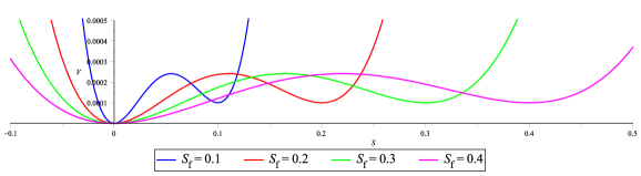
Figure 1: (color online). The quartic potential $V\left(S\right)=\frac{3V_{\mathrm{f}}}{\beta S_{\mathrm{f}}^{4}}S^{4}-\frac{2\left(\beta+3\right)V_{\mathrm{f}}}{\beta S_{\mathrm{f}}^{3}}S^{3}+\frac{3\left(\beta+1\right)V_{\mathrm{f}}}{\beta S_{\mathrm{f}}^{2}}S^{2}$; expressed in terms of the false vacuum field $S_{\mathrm{f}}=\sqrt{4\pi}\phi_{\mathrm{f}}$, the vacuum energy of the false vacuum $V_{\mathrm{f}}$ and a free parameter $\beta$. The patterns of the potential are shown for $\beta=0.1$, $V_{\mathrm{f}}=10^{-4}$ and $S_{\mathrm{f}}=\sqrt{4\pi}\phi_{\mathrm{f}}=$ (1) $0.1$, (2) $0.2$, (3) $0.3$, (4) $0.4$. (Credit: Hwang et al. Hwang )

Figure 2: (color online). The numerical solutions $S\left(u,v\right)=\sqrt{4\pi}\phi\left(u,v\right)$ obtained with the potential from Figure 1; with various false vacuum field values, $S_{\mathrm{f}}=\sqrt{4\pi}\phi_{\mathrm{f}}=$ (1) $0.1$, (2) $0.2$, (3) $0.3$, (4) $0.4$. (Credit: Hwang et al. Hwang )

III Gravitational waves from bubble collisions

In Section II we have built a system of two equal-sized colliding bubbles in curved spacetime by means of a CDL instanton model, considering the potential given by Eq. (7) Hwang . Now, we consider that the a present observer lives in the true vacuum region of one of the two bubbles and that signatures of bubble collisions which took place in the distant past are being carried to the present observer via GWs. Here we assume that the distance between the center of collision region and the observer can be arbitrarily large (within the size of our universe), and thus that the time for a collision event, which is the retarded time to the present observer, can be quite far in the distant past; namely, $t_{\mathrm{R}}=t_{\mathrm{P}}-r/c\ll t_{\mathrm{P}}$, where $t_{\mathrm{R}}$ denotes the retarded time, $t_{\mathrm{P}}$ the present time and $r$ the distance. Therefore, our bubble collision may be regarded as a localized event, as long as the observer is reasonably far away from the collision region. In Figure 3 a causal relationship between two colliding bubbles and an observer is depicted using a null-cone. Here collision events that took place in the distant past are placed within the intersection of the timelike zone (green-colored region) of a null-cone (green dashed lines) and the ‘diamond’ zone (region enclosed by black dashed lines): all the collision events as our GW sources, namely the collisions in Figure 2 (strong collisions in the initial-to-intermediate stage) and the collisions to be discussed in Subsection III.2 later (weak collisions in the final stage) should be considered to have taken place within this intersection .

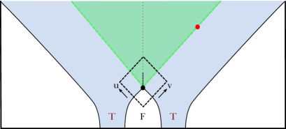
Figure 3: (color online). A causal relationship between two colliding bubbles and an observer: Gravitational waves from bubble collisions can be observed by a distant observer (red spot) who is in the causal future of a collision event (black spot). The dotted vertical line inside the timelike zone (green-colored region) of a null-cone (green dashed lines) represents the time-axis, along which bubble collisions took place in the distant past; within the intersection of the timelike zone of the null-cone and the ‘diamond’ zone (region enclosed by black dashed lines). $u$ and $v$ represent the double-null coordinates as defined in Section II. T and F denote a true vacuum and a false vacuum, respectively.

In the above scenario, our GWs from bubble collisions can be computed in a straightforward manner: by integrating the energy-momentum tensors combined with a Green’s function over the volume of the wave sources, where the energy-momentum tensors are expressed in terms of the scalar field, the local geometry and the potential by means of Eqs. (3), (5) and (8); therefore, containing all necessary information about the bubble collisions. A mathematical description of this computation is given as follows. In the transverse trace-free (TT) gauge, GWs, as derived from the perturbed Einstein equations in linearized gravity, can be expressed as

$$h_{ij}^{\mathrm{TT}}\left(t,\mathbf{x}\right)=\overline{h}_{ij}^{\mathrm{TT}}\left(t,\mathbf{x}\right)=\frac{4G}{c^{4}}\Lambda_{ij,kl}\left(\mathbf{n}\right)\int d^{3}x^{\prime}\frac{1}{\left|\mathbf{x-x}^{\prime}\right|}T^{kl}\left(t-\frac{\left|\mathbf{x-x}^{\prime}\right|}{c},\mathbf{x}^{\prime}\right)\,,$$ (9)

where $\overline{h}_{ij}\equiv h_{ij}-\frac{1}{2}\delta_{ij}h_{k}^{k}$ and the unit vector $\mathbf{n}$ denotes the propagation direction of the waves, and the projection tensor for gravitational radiation,

$$\Lambda_{ij,kl}\left(\mathbf{n}\right)\equiv P_{ik}P_{jl}-\frac{1}{2}P_{ij}P_{kl}$$ (10)

with

$$P_{ij}=\delta_{ij}-n_{i}n_{j}\,.$$ (11)

We find that the computation would be technically quite difficult with the integral as it is in Eq. (9): the way the source point $\mathbf{x}^{\prime}$ (integration variable) is combined with the field point $\mathbf{x}$ in the integrand would make our calculation quite intractable. However, expressing the integral in expansion, we obtain a more computationally favorable form:

$$h_{ij}^{\mathrm{TT}}\left(t,\mathbf{x}\right) = \frac{4G}{c^{4}r}\Lambda_{ij,kl}\left(\mathbf{n}\right)\left[\int d^{3}x^{\prime}T^{kl}\left(t_{\mathrm{R}},\mathbf{x}^{\prime}\right)\right.$$ (12)

$$\left.+\frac{1}{c}n^{m}\frac{d}{dt_{\mathrm{R}}}\int d^{3}x^{\prime}T^{kl}\left(t_{\mathrm{R}},\mathbf{x}^{\prime}\right)x_{m}^{\prime}\right.$$

$$\left.+\frac{1}{2c^{2}}n^{m}n^{p}\frac{d^{2}}{dt_{\mathrm{R}}^{2}}\int d^{3}x^{\prime}T^{kl}\left(t_{\mathrm{R}},\mathbf{x}^{\prime}\right)x_{m}^{\prime}x_{p}^{\prime}+\cdots\right]_{t_{\mathrm{R}}=t-r/c}\,,$$

where $r=\left|\mathbf{x}\right|$ and $t_{\mathrm{R}}=t-r/c$ denotes the retarded time. In particular, the computation resulting from the first term alone in the square bracket in Eq. (12) is called the “quadrupole approximation”. The next terms will provide corrections to this computation.

III.1 Computation of gravitational waves in the quadrupole approximation

The complete information about the motion of the colliding two-bubble system is encoded in the scalar field solution $S=\sqrt{4\pi}\phi$, as given by Figure 2, and thus is carried by the energy-momentum tensors through Eq. (3): to be precise, the energy-momentum tensors are comprised of the scalar field $S$ and the geometry $g_{\mu\nu}$, which are obtained by solving Eqs. (2) and (4) simultaneously Hwang . As described by Eqs. (9) and (12), GWs from the system are computed with the energy-momentum tensors being the sources. It is believed that the two bubbles will be in highly relativistic motion when they collide Hawking . In view of this, corrections due to the next-to-leading order terms in Eq. (12) should not be disregarded if one aims to compute GWs from the system accurately. However, although not perfectly accurate, the leading order term alone in Eq. (12) provides the “quadrupole approximation” of GWs:

$${}_{\mathrm{Q}}h_{ij}^{\mathrm{TT}}\left(t,\mathbf{x}\right)=\frac{4}{r}\Lambda_{ij,kl}\left(\mathbf{n}\right)I_{kl}\left(t_{\mathrm{R}}\right)\,,$$ (13)

where we have adopted the unit convention $c=G=1$, and

$$I_{kl}\left(t_{\mathrm{R}}\right)\equiv\int d^{3}x^{\prime}T^{kl}\left(t_{\mathrm{R}},\mathbf{x}^{\prime}\right)\,.$$ (14)

Throughout this paper our computation is carried out only from this piece. Our main purpose is to provide qualitative insights into patterns of GWs from the colliding two-bubble system in time domain, and the next-to-leading order corrections in Eq. (12) are disregarded in our analysis.

Following Ref. Kosowsky , we can reduce the amount of computation in a great deal. As described in Subsection II.1, we choose the $x$-axis to coincide with the line adjoining the centers of the two bubbles. With the axial symmetry about the $x$-axis, the off-diagonal components are zero and we can put $I_{kl}$ in the form,

$$I_{kl}=D\delta_{kl}+\triangle\delta_{kx}\delta_{lx}\,.$$ (15)

Here, the first term turns out to be

$$D=\frac{1}{2}\left(I_{yy}+I_{zz}\right)\,,$$ (16)

which does not contribute to gravitational radiation due to Eqs. (10) and (11). The second term is given by

$$\triangle=I_{xx}-\frac{1}{2}\left(I_{yy}+I_{zz}\right)\,.$$ (17)

Therefore, $I_{kl}$ is practically equivalent to $\triangle\delta_{kx}\delta_{lx}$:

$$I_{kl}\sim\delta_{kx}\delta_{lx}\left[I_{xx}-\frac{1}{2}\left(I_{yy}+I_{zz}\right)\right]\,.$$ (18)

Then by Eqs. (14) and (18) we may express

$$I_{kl}\left(t_{\mathrm{R}}\right)=\delta_{kx}\delta_{lx}\int d^{3}x^{\prime}\left[T^{xx}\left(t_{\mathrm{R}},\mathbf{x}^{\prime}\right)-\frac{1}{2}\left[T^{yy}\left(t_{\mathrm{R}},\mathbf{x}^{\prime}\right)+T^{zz}\left(t_{\mathrm{R}},\mathbf{x}^{\prime}\right)\right]\right]\,.$$ (19)

Now, recall from Subsection II.1 that in the flat spacetime we define the hyperbolic coordinates $\tau$, $\chi$, $\theta$ by

$$t_{\mathrm{R}} = \tau\cosh\chi\,,$$ (20)

$$y = \tau\sinh\chi\sin\theta\,,$$ (21)

$$z = \tau\sinh\chi\cos\theta\,,$$ (22)

so that

$$\tau^{2}=t_{\mathrm{R}}^{2}-\rho^{2},$$ (23)

where $0\leq\chi<\infty$, $0\leq\theta<2\pi$ and $\rho\equiv\sqrt{y^{2}+z^{2}}$. In these coordinates the flat spacetime metric takes the form,

$$ds^{2}=-d\tau^{2}+dx^{2}+\tau^{2}\left(d\chi^{2}+\sinh^{2}\chi d\theta^{2}\right)\,.$$ (24)

In this geometry, however, the scalar field solution is independent of the coordinates $\chi$ and $\theta$ and is expressed in the coordinates $\left(\tau,x\right)$ only; namely, $\phi\left(\tau,x\right)$ Hawking ; Kosowsky . Taking this into account, we should rewrite the volume element for the integral (19) as

$$d^{3}x=dx\rho d\rho d\theta=-dx\tau d\tau d\theta\,,$$ (25)

which is defined at the instant $t_{\mathrm{R}}$ by means of Eq. (23).

From Eq. (23) we see that $\tau$ has an upper bound $t_{\mathrm{R}}$ with $\rho=0$. This represents the exterior surface of the bubble walls, i.e.

$$\tau=t_{\mathrm{R}}.$$ (26)

However, the interior surface is found from Eq. (23) to be

$$\tau=t_{\mathrm{R}}-\frac{\eta^{2}}{8t_{\mathrm{R}}}+\mathcal{O}\left(\frac{\eta^{4}}{t_{\mathrm{R}}^{3}}\right)\,,$$ (27)

given a wall thickness $\eta\sim 2\rho\ll t_{\mathrm{R}}$. Then from Eqs. (19), (25), (26) and (27) we can compute $I_{kl}\left(t_{\mathrm{R}}\right)$ effectively out of a volume piece $\mathcal{V}$:

$$I_{kl}\left(t_{\mathrm{R}}\right) = \delta_{kx}\delta_{lx}\int_{\mathcal{V}}d^{3}x^{\prime}\left[T_{xx}-\frac{1}{2}\left(T_{yy}+T_{zz}\right)\right]$$ (28)

$$= 2\pi\delta_{kx}\delta_{lx}\int_{t_{\mathrm{R}}-\eta^{2}/\left(8t_{\mathrm{R}}\right)}^{t_{\mathrm{R}}}d\tau^{\prime}\tau^{\prime}\int_{-x_{\mathrm{o}}}^{x_{\mathrm{o}}}dx^{\prime}\left[T_{xx}-\frac{1}{2}\left(T_{yy}+T_{zz}\right)\right]+\mathcal{O}\left(\frac{\eta^{4}}{t_{\mathrm{R}}^{3}}\right)$$

$$= \frac{\pi}{4}\delta_{kx}\delta_{lx}\eta^{2}\int_{-x_{\mathrm{o}}}^{x_{\mathrm{o}}}dx^{\prime}\left[T_{xx}-\frac{1}{2}\left(T_{yy}+T_{zz}\right)\right]_{\tau=t_{\mathrm{R}}}+\mathcal{O}\left(\frac{\eta^{4}}{t_{\mathrm{R}}^{3}}\right)\,,$$

where the volume piece $\mathcal{V}$ is defined from a thin cylindrical shell in motion, having the thickness $\eta^{2}/\left(8t_{\mathrm{R}}\right)$, extending along the $x$-axis, by means of Eqs. (26) and (27): from $t_{\mathrm{R}}-\eta^{2}/\left(8t_{\mathrm{R}}\right)+\mathcal{O}\left(\eta^{4}/t_{\mathrm{R}}^{3}\right)\leq\tau\leq$ $t_{\mathrm{R}}$ we find $\mathcal{V}=\Delta x\left|\tau\Delta\tau\right|\Delta\theta=\frac{\pi}{4}\eta^{2}\Delta x\left[1+\mathcal{O}\left(\eta^{2}/t_{\mathrm{R}}^{2}\right)\right]$, and the limit of the integral $x_{\mathrm{o}}=\Delta x/2$ should be chosen to be sufficiently large such that collision effects be fully covered in numerical integration . Following Ref. Hawking , we estimate a bubble wall thickness $\eta$, assuming that the walls will be highly relativistic when they collide, having the Lorentz factor $\gamma$:

$$\eta\sim\frac{3}{2}\phi_{\mathrm{f}}/\left(\xi^{2}\gamma\right)\sim\frac{3}{2}\phi_{\mathrm{f}}^{2}/\left(b\epsilon^{4}\right)\,,$$ (29)

where $\phi_{\mathrm{f}}$ denotes the scalar field value at the false vacuum and $\xi^{4}$ the effective height of the potential barrier between the two minima, and the Lorentz factor $\gamma=b\epsilon^{4}/\left(\xi^{2}\phi_{\mathrm{f}}\right)$ with $2b$ representing the separation of the bubbles and $\epsilon^{4}$ the potential difference between the two minima (which is equivalent to $V_{\mathrm{f}}$ in our analysis in Subsection II.2) Hawking .

However, as described in Subsection II.2, our scalar field $S=\sqrt{4\pi}\phi$ is obtained by solving Eqs. (2) and (8) simultaneously, using the ansatz given by Eq. (5), in the coordinates $\left(u,v,\chi,\theta\right)$. Then by Eq. (3) the energy-momentum tensors should be expressed in the same coordinates. Now, due to the definitions of $u$ and $v$ in the flat spacetime limit, and by Eqs. (20), (21) and (22) we have

$$u = \tau-x=\sqrt{t_{\mathrm{R}}^{2}-\left(y^{2}+z^{2}\right)}-x\,,$$ (30)

$$v = \tau+x=\sqrt{t_{\mathrm{R}}^{2}-\left(y^{2}+z^{2}\right)}+x\,,$$ (31)

$$\chi = \tanh^{-1}\left(\sqrt{\frac{y^{2}+z^{2}}{t_{\mathrm{R}}^{2}}}\right)\,.$$ (32)

Using these relations, we find

$$T_{xx} = T_{uu}\left(\frac{\partial u}{\partial x}\right)^{2}+2T_{uv}\frac{\partial u}{\partial x}\frac{\partial v}{\partial x}+T_{vv}\left(\frac{\partial v}{\partial x}\right)^{2}+T_{\chi\chi}\left(\frac{\partial\chi}{\partial x}\right)^{2}$$ (33)

$$= T_{uu}-2T_{uv}+T_{vv},$$

$$T_{yy} = T_{uu}\left(\frac{\partial u}{\partial y}\right)^{2}+2T_{uv}\frac{\partial u}{\partial y}\frac{\partial v}{\partial y}+T_{vv}\left(\frac{\partial v}{\partial y}\right)^{2}+T_{\chi\chi}\left(\frac{\partial\chi}{\partial y}\right)^{2}$$ (34)

$$= \frac{y^{2}}{t_{\mathrm{R}}^{2}-\left(y^{2}+z^{2}\right)}\left(T_{uu}+2T_{uv}+T_{vv}\right)+\frac{t_{\mathrm{R}}^{2}y^{2}}{\left[t_{\mathrm{R}}^{2}-\left(y^{2}+z^{2}\right)\right]^{2}\left(y^{2}+z^{2}\right)}T_{\chi\chi}\,,$$

$$T_{zz} = T_{uu}\left(\frac{\partial u}{\partial z}\right)^{2}+2T_{uv}\frac{\partial u}{\partial z}\frac{\partial v}{\partial z}+T_{vv}\left(\frac{\partial v}{\partial z}\right)^{2}+T_{\chi\chi}\left(\frac{\partial\chi}{\partial z}\right)^{2}$$ (35)

$$= \frac{z^{2}}{t_{\mathrm{R}}^{2}-\left(y^{2}+z^{2}\right)}\left(T_{uu}+2T_{uv}+T_{vv}\right)+\frac{t_{\mathrm{R}}^{2}z^{2}}{\left[t_{\mathrm{R}}^{2}-\left(y^{2}+z^{2}\right)\right]^{2}\left(y^{2}+z^{2}\right)}T_{\chi\chi}\,.$$

Substituting Eqs. (33), (34) and (35) into Eq. (28), we obtain

$$I_{kl}\left(t_{\mathrm{R}}\right)=\frac{\pi}{4}\delta_{kx}\delta_{lx}\eta^{2}\int_{-x_{\mathrm{o}}}^{x_{\mathrm{o}}}dx^{\prime}\left[T_{uu}-2T_{uv}+T_{vv}-\frac{1}{2t_{\mathrm{R}}^{2}}T_{\chi\chi}\right]_{t_{\mathrm{R}}}+\mathcal{O}\left(\frac{\eta^{4}}{t_{\mathrm{R}}^{3}}\right)\,,$$ (36)

where the subscript $t_{\mathrm{R}}$ outside the square bracket means that the double-null coordinates $\left(u,v\right)$ are defined at $\tau=t_{\mathrm{R}}$; namely, $u=t_{\mathrm{R}}-x$ and $v=t_{\mathrm{R}}+x$. In the actual computation of Eq. (36), we integrate $T_{uu}\left(u,v\right)$, $T_{uv}\left(u,v\right)$, $T_{vv}\left(u,v\right)$ and $T_{\chi\chi}\left(u,v\right)$, which are constructed out of the scalar field solution $S\left(u,v\right)=\sqrt{4\pi}\phi\left(u,v\right)$, the geometry solution $g_{uv}\left(u,v\right)$, $g_{\chi\chi}\left(u,v\right)$, $g_{\theta\theta}\left(u,v\right)$ and the potential $V\left(S\right)$ via Eq. (3). Then we need to change the variable of integration, from $x$ to $u$ or $v$. Using the relations $u=t_{\mathrm{R}}-x$ and $v=t_{\mathrm{R}}+x$, we can convert

$$dx=-du\text{ \ \ or \ }dx=dv.$$ (37)

Then we may rewrite

$$\int_{-x_{\mathrm{o}}}^{x_{\mathrm{o}}}dx^{\prime}~{}T_{ab}\left(u,v\right) = \int_{t_{\mathrm{R}}-x_{\mathrm{o}}}^{t_{\mathrm{R}}+x_{\mathrm{o}}}du~{}T_{ab}\left(u,2t_{\mathrm{R}}-u\right)=\int_{t_{\mathrm{R}}-x_{\mathrm{o}}}^{t_{\mathrm{R}}+x_{\mathrm{o}}}dv~{}T_{ab}\left(2t_{\mathrm{R}}-v,v\right)$$ (38)

$$= 2\int_{0}^{x_{\mathrm{o}}}du~{}T_{ab}\left(t_{\mathrm{R}}+u,t_{\mathrm{R}}-u\right)=2\int_{0}^{x_{\mathrm{o}}}dv~{}T_{ab}\left(t_{\mathrm{R}}-v,t_{\mathrm{R}}+v\right)\,,$$

where $T_{ab}$ represents any of $T_{uu}$, $T_{uv}$, $T_{vv}$ and $T_{\chi\chi}$, and the expressions in the second line have been obtained via translations, $u\rightarrow u-t_{\mathrm{R}}$ and $v\rightarrow v-t_{\mathrm{R}}$. Then by Eqs. (36) and (38) $I_{kl}\left(t_{\mathrm{R}}\right)$ can be expressed as

$$I_{kl}\left(t_{\mathrm{R}}\right) = \frac{\pi}{2}\delta_{kx}\delta_{lx}\eta^{2}\left[\int_{0}^{x_{\mathrm{o}}}du~{}T_{uu}\left(t_{\mathrm{R}}\pm u,t_{\mathrm{R}}\mp u\right)-2\int_{0}^{x_{\mathrm{o}}}du~{}T_{uv}\left(t_{\mathrm{R}}\pm u,t_{\mathrm{R}}\mp u\right)\right.$$ (39)

$$\!\!\left.+\int_{0}^{x_{\mathrm{o}}}du~{}T_{vv}\left(t_{\mathrm{R}}\pm u,t_{\mathrm{R}}\mp u\right)-\frac{1}{2t_{\mathrm{R}}^{2}}\int_{0}^{x_{\mathrm{o}}}du~{}T_{\chi\chi}\left(t_{\mathrm{R}}\pm u,t_{\mathrm{R}}\mp u\right)\right]+\mathcal{O}\left(\frac{\eta^{4}}{t_{\mathrm{R}}^{3}}\right)\,.$$

If the wall thickness $\eta$ can be taken sufficiently small in Eq. (39), then by Eq. (13) we can compute the bubble-collision-induced GWs in the quadrupole approximation as

$${}_{\mathrm{Q}}h_{ij}^{\mathrm{TT}}\left(t,\mathbf{x}\right) \approx \frac{2\pi}{r}\eta^{2}\Lambda_{ij,kl}\left(\mathbf{n}\right)\delta_{kx}\delta_{lx}$$ (40)

$$\times\text{ }\left[\int_{0}^{x_{\mathrm{o}}}du~{}T_{uu}\left(t_{\mathrm{R}}\pm u,t_{\mathrm{R}}\mp u\right)-2\int_{0}^{x_{\mathrm{o}}}du~{}T_{uv}\left(t_{\mathrm{R}}\pm u,t_{\mathrm{R}}\mp u\right)\right.$$

$$\left.+\int_{0}^{x_{\mathrm{o}}}du~{}T_{vv}\left(t_{\mathrm{R}}\pm u,t_{\mathrm{R}}\mp u\right)-\frac{1}{2t_{\mathrm{R}}^{2}}\int_{0}^{x_{\mathrm{o}}}du~{}T_{\chi\chi}\left(t_{\mathrm{R}}\pm u,t_{\mathrm{R}}\mp u\right)\right]\,.$$

Now, without loss of generality we may choose

$$\mathbf{n=}{\left(n_{x},n_{y},n_{z}\right)=\left(\cos\vartheta,\sin\vartheta,0\right)}\,,$$ (41)

where $\vartheta$ denotes the angle of propagation taken from the $x$-axis. From this it follows that

$$\Lambda_{ij,kl}\left(\mathbf{n}\right)\delta_{kx}\delta_{lx}=\delta_{ix}\delta_{jx}-2\delta_{ix}n_{j}\cos\vartheta+\frac{1}{2}n_{i}n_{j}\left(1+\cos^{2}\vartheta\right)-\frac{1}{2}\delta_{ij}\sin^{2}\vartheta\,,$$ (42)

due to Eqs. (10) and (11). Substituting this into Eq. (40), we finally express

$${}_{\mathrm{Q}}h_{ij}^{\mathrm{TT}}\left(t,\mathbf{x}\right) \approx \frac{2\pi}{r}\eta^{2}\left[\delta_{ix}\delta_{jx}-2\delta_{ix}n_{j}\cos\vartheta+\frac{1}{2}n_{i}n_{j}\left(1+\cos^{2}\vartheta\right)-\frac{1}{2}\delta_{ij}\sin^{2}\vartheta\right]$$ (43)

$$\times\text{ }\left[\int_{0}^{x_{\mathrm{o}}}du~{}T_{uu}\left(t_{\mathrm{R}}\pm u,t_{\mathrm{R}}\mp u\right)-2\int_{0}^{x_{\mathrm{o}}}du~{}T_{uv}\left(t_{\mathrm{R}}\pm u,t_{\mathrm{R}}\mp u\right)\right.$$

$$\left.+\int_{0}^{x_{\mathrm{o}}}du~{}T_{vv}\left(t_{\mathrm{R}}\pm u,t_{\mathrm{R}}\mp u\right)-\frac{1}{2t_{\mathrm{R}}^{2}}\int_{0}^{x_{\mathrm{o}}}du~{}T_{\chi\chi}\left(t_{\mathrm{R}}\pm u,t_{\mathrm{R}}\mp u\right)\right]\,,$$

where $t_{\mathrm{R}}=t-r=t-\left|\mathbf{x}\right|$, and the wall thickness $\eta$ can be specified by means of Eq. (29); namely, in terms of the quantities for the bubble collision profiles, such as the false vacuum field $\phi_{\mathrm{f}}$ (equivalent to $S_{\mathrm{f}}/\sqrt{4\pi}$), the potential difference between the two minima $\epsilon^{4}$ (equivalent to $V_{\mathrm{f}}$) and half the separation of the bubbles $b$ Hawking .

RESULT 1: The numerical computations of Eq. (43) are presented in Figure 4; with various false vacuum field values, $S_{\mathrm{f}}=\sqrt{4\pi}\phi_{\mathrm{f}}=$ (1) $0.1$, (2) $0.2$, (3) $0.3$, (4) $0.4$, in accordance with the scalar field solutions as presented by Figure 2. Due to Eqs. (29) and (43), the amplitude of our GWs ${}_{\mathrm{Q}}h^{\mathrm{TT}}\left(t\right)$ scales as $\phi_{\mathrm{f}}^{4}$ if the other conditions, $\epsilon^{4}$ and $b$ are kept the same. Thus, with $S_{\mathrm{f}}=$ (1) $0.1$, (2) $0.2$, (3) $0.3$, (4) $0.4$, the amplitude scales as (1) $1$, (2) $2^{4}$, (3) $3^{4}$, (4) $4^{4}$. The frequency of the waves is modulating due to the non-linearity of the collision dynamics in the all four cases of $S_{\mathrm{f}}$, (1) - (4). However, the modulating frequency increases overall as $S_{\mathrm{f}}$ increases, which is analogous to the tendency exhibited by $S\left(u,v\right)=\sqrt{4\pi}\phi\left(u,v\right)$ as shown in Figure 2. In Figure 4, we present ${}_{\mathrm{Q}}h^{\mathrm{TT}}\left(t\right)r/\left(2\pi\eta^{2}\right)$ instead of ${}_{\mathrm{Q}}h^{\mathrm{TT}}\left(t\right)$, and thus all the waveforms are plotted in the same scale. One should note here that our actual numerical data of the energy-momentum tensors $T_{ab}$ for Eq. (43) have been obtained via Eq. (3) after solving Eqs. (2) and (4) simultaneously Hwang . Therefore, our $T_{ab}$ contain the full physical information about the bubble collisions in terms of the scalar field $S=\sqrt{4\pi}\phi$, the geometry $g_{ab}$ and the potential $V\left(S\right)$; with the radiation reaction effects included in $S$ and $g_{ab}$ .

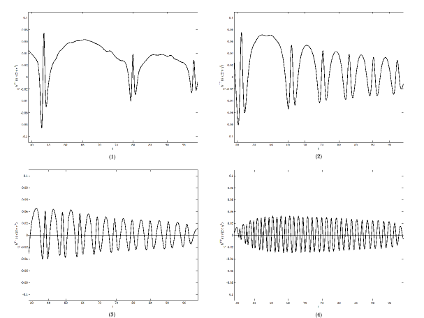
Figure 4: The numerical plots of ${}_{\mathrm{Q}}h^{\mathrm{TT}}\left(t\right)r/\left(2\pi\eta^{2}\right)$ with various false vacuum field values, $S_{\mathrm{f}}=\sqrt{4\pi}\phi_{\mathrm{f}}=$ (1) $0.1$, (2) $0.2$, (3) $0.3$, (4) $0.4$. As $\eta^{2}\sim\phi_{\mathrm{f}}^{4}$, the amplitude of ${}_{\mathrm{Q}}h^{\mathrm{TT}}\left(t\right)$ should scale as (1) $1$, (2) $2^{4}$, (3) $3^{4}$, (4) $4^{4}$.

III.2 A simplified method to compute gravitational waves in the quadrupole approximation

Ref. Kosowsky presents a simplified method to compute the GWs ${}_{\mathrm{Q}}h_{ij}^{\mathrm{TT}}\left(t,\mathbf{x}\right)$ of Eq. (13) by neglecting the gravitational effects on the bubbles: namely, $g_{\mu\nu}$ in Eq. (3) is replaced by $\eta_{\mu\nu}$, assuming that the bubbles are in flat spacetime. Then Eq. (14) can be simplified as

$$I_{kl}\left(t_{\mathrm{R}}\right)=\int d^{3}x^{\prime}T^{kl}\left(t_{\mathrm{R}},\mathbf{x}^{\prime}\right)=\int d^{3}x^{\prime}\partial_{k}\phi\left(t_{\mathrm{R}},\mathbf{x}^{\prime}\right)\partial_{l}\phi\left(t_{\mathrm{R}},\mathbf{x}^{\prime}\right)\,,$$ (44)

where the energy-momentum tensors from Eq. (3) have been reduced; $T_{ij}\rightarrow\partial_{i}\phi\partial_{j}\phi$ because the terms proportional to $\delta_{ij}$ in $T_{ij}$ makes no contribution to gravitational radiation in Eq. (13) due to the property of Eq. (10); namely, $\Lambda_{ij,kl}\delta_{ij}=0$ Kosowsky .

By Eqs. (18) and (44) we have

$$I_{kl} = \delta_{kx}\delta_{lx}\int d^{3}x^{\prime}\left[\left(\frac{\partial\phi}{\partial x^{\prime}}\right)^{2}-\frac{1}{2}\left(\frac{\partial\phi}{\partial y^{\prime}}\right)^{2}-\frac{1}{2}\left(\frac{\partial\phi}{\partial z^{\prime}}\right)^{2}\right]$$ (45)

$$= \delta_{kx}\delta_{lx}\int d^{3}x^{\prime}\left[\left(\frac{\partial\phi}{\partial x^{\prime}}\right)^{2}-\frac{1}{2}\left(\frac{\partial\phi}{\partial\rho^{\prime}}\right)^{2}\right]\,.$$

Using Eq. (23), we can modify

$$\left(\frac{\partial\phi}{\partial\rho}\right)^{2}=\left(\frac{\partial\phi}{\partial\tau}\right)^{2}\left(\frac{\partial\tau}{\partial\rho}\right)^{2}=\frac{t_{\mathrm{R}}^{2}-\tau^{2}}{\tau^{2}}\left(\frac{\partial\phi}{\partial\tau}\right)^{2}\,.$$ (46)

Then in the same manner as described above by Eq. (28), the integral $I_{kl}\left(t_{\mathrm{R}}\right)$ is computed out of the volume piece $\mathcal{V}=\Delta x\left|\tau\Delta\tau\right|\Delta\theta=\frac{\pi}{4}\eta^{2}\Delta x\left[1+\mathcal{O}\left(\eta^{2}/t_{\mathrm{R}}^{2}\right)\right]$:

$$I_{kl}\left(t_{\mathrm{R}}\right) = \delta_{kx}\delta_{lx}\int_{\mathcal{V}}d^{3}x^{\prime}\left[\left(\frac{\partial\phi}{\partial x^{\prime}}\right)^{2}-\frac{1}{2}\left(\frac{\partial\phi}{\partial\rho^{\prime}}\right)^{2}\right]$$ (47)

$$= 2\pi\delta_{kx}\delta_{lx}\int_{t_{\mathrm{R}}-\eta^{2}/\left(8t_{\mathrm{R}}\right)}^{t_{\mathrm{R}}}d\tau^{\prime}\tau^{\prime}\int_{-x_{\mathrm{o}}}^{x_{\mathrm{o}}}dx^{\prime}\left[\left(\frac{\partial\phi}{\partial x^{\prime}}\right)^{2}-\frac{t_{\mathrm{R}}^{2}-\tau^{\prime 2}}{2\tau^{\prime 2}}\left(\frac{\partial\phi}{\partial\tau^{\prime}}\right)^{2}\right]+\mathcal{O}\left(\frac{\eta^{4}}{t_{\mathrm{R}}^{3}}\right)$$

$$= \frac{\pi}{2}\delta_{kx}\delta_{lx}\eta^{2}\int_{0}^{x_{\mathrm{o}}}dx^{\prime}\left(\frac{\partial\phi}{\partial x^{\prime}}\right)_{\tau=t_{\mathrm{R}}}^{2}+\mathcal{O}\left(\frac{\eta^{4}}{t_{\mathrm{R}}^{3}}\right)\,.$$

If the wall thickness $\eta$ can be taken sufficiently small in Eq. (47), by Eqs. (13) and (47) we can compute the bubble-collision-induced GWs in the quadrupole approximation as

$${}_{\mathrm{Q}}h_{ij}^{\mathrm{TT}}\left(t,\mathbf{x}\right)\approx\frac{2\pi}{r}\Lambda_{ij,kl}\left(\mathbf{n}\right)\delta_{kx}\delta_{lx}\eta^{2}\int_{0}^{x_{\mathrm{o}}}dx^{\prime}\left(\frac{\partial\phi}{\partial x^{\prime}}\right)_{\tau=t_{\mathrm{R}}}^{2}\,.$$ (48)

Substituting Eq. (42) into Eq. (48), we finally express

$${}_{\mathrm{Q}}h_{ij}^{\mathrm{TT}}\left(t,\mathbf{x}\right) \approx \frac{2\pi}{r}\eta^{2}\left[\delta_{ix}\delta_{jx}-2\delta_{ix}n_{j}\cos\vartheta+\frac{1}{2}n_{i}n_{j}\left(1+\cos^{2}\vartheta\right)-\frac{1}{2}\delta_{ij}\sin^{2}\vartheta\right]$$ (49)

$$\times\int_{0}^{x_{\mathrm{o}}}dx^{\prime}\left(\frac{\partial\phi}{\partial x^{\prime}}\right)_{\tau=t_{\mathrm{R}}}^{2}\,,$$

where $t_{\mathrm{R}}=t-r=t-\left|\mathbf{x}\right|$, and $\eta$ is specified by Eq. (29).

RESULT 2: Toward the end of the bubble collisions, $\tau\gg 1$, the scalar field oscillates around the true vacuum state, i.e. $\left|\phi\right|\ll 1$, being nearly monochromatic. Then we can approximate Eq. (8) as

$$\square\phi\left(\tau,x\right)\approx\frac{6\left(\beta+1\right)V_{\mathrm{f}}}{\beta S_{\mathrm{f}}^{2}}\phi\left(\tau,x\right)\,,$$ (50)

where we have replaced the curved spacetime Laplacian $\nabla^{2}$ by the flat spacetime d’Alembertian $\square\equiv-\partial^{2}/\partial\tau^{2}-\left(2/\tau\right)\partial/\partial\tau+\partial^{2}/\partial x^{2}$, neglecting the gravitational effects on the bubbles to simplify the problem . With the help of Ref. Polyanin , we obtain a solution for Eq. (50):

$$\phi\left(\tau,x\right)=\phi_{\mathrm{o}}\frac{J_{1}\left(\omega_{\mathrm{t}}\sqrt{\tau^{2}-x^{2}}\right)}{\omega_{\mathrm{t}}\sqrt{\tau^{2}-x^{2}}}\,,$$ (51)

where $J_{n}$ denotes the Bessel function of the first kind, $\omega_{\mathrm{t}}\equiv\sqrt{6\left(\beta+1\right)V_{\mathrm{f}}/\left(\beta S_{\mathrm{f}}^{2}\right)}$ represents the ‘terminal’ frequency of the bubble collisions, and $\phi_{\mathrm{o}}$ is the amplitude which is determined by the initial conditions of the field. Substituting Eq. (51) into Eq. (49), the GWs emitted from the bubble collisions in the final stage can be computed. Figure 5 shows the GWs ${}_{\mathrm{Q}}h^{\mathrm{TT}}\left(t\right)r/\left(2\pi\eta^{2}\right)$ computed with various false vacuum field values, $S_{\mathrm{f}}=\sqrt{4\pi}\phi_{\mathrm{f}}=$ (1) $0.1$, (2) $0.2$, (3) $0.3$, (4) $0.4$. Corresponding to the field values are the frequencies, $\omega_{\mathrm{t}}\simeq$ (1) $0.8124$, (2) $0.4062$, (3) $0.2708$, (4) $0.2031$ $\sim$ (1) $1$, (2) $1/2$, (3) $1/3$, (4) $1/4$, as can be seen from Figure 5. Also, the amplitude of ${}_{\mathrm{Q}}h^{\mathrm{TT}}\left(t\right)r/\left(2\pi\eta^{2}\right)$ scales as (1) $1$, (2) $2$, (3) $3$, (4) $4$ due to the factor $\omega_{\mathrm{t}}^{-1}\sim S_{\mathrm{f}}$, as can be seen from Figure 5. Then the amplitude of ${}_{\mathrm{Q}}h^{\mathrm{TT}}\left(t\right)$ should scale as $\eta^{2}\omega_{\mathrm{t}}^{-1}\sim S_{\mathrm{f}}^{5}\sim$ (1) $1$, (2) $2^{5}$, (3) $3^{5}$, (4) $4^{5}$.

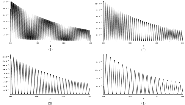
Figure 5: Plots of ${}_{\mathrm{Q}}h^{\mathrm{TT}}\left(t\right)r/\left(2\pi\eta^{2}\right)$ computed via the expression in Eq. (49), with $\phi$ given by Eq. (51). Corresponding to the false vacuum field values, $S_{\mathrm{f}}=\sqrt{4\pi}\phi_{\mathrm{f}}=$ (1) $0.1$, (2) $0.2$, (3) $0.3$, (4) $0.4$, are the frequencies, $\omega_{\mathrm{t}}\simeq$ (1) $0.8124$, (2) $0.4062$, (3) $0.2708$, (4) $0.2031$ $\sim$ (1) $1$, (2) $1/2$, (3) $1/3$, (4) $1/4$. And the amplitude of ${}_{\mathrm{Q}}h^{\mathrm{TT}}\left(t\right)r/\left(2\pi\eta^{2}\right)$ scales as (1) $1$, (2) $2$, (3) $3$, (4) $4$ due to the factor $\omega_{\mathrm{t}}^{-1}\sim S_{\mathrm{f}}$. Then the amplitude of ${}_{\mathrm{Q}}h^{\mathrm{TT}}\left(t\right)$ should scale as $\eta^{2}\omega_{\mathrm{t}}^{-1}\sim S_{\mathrm{f}}^{5}\sim$ (1) $1$, (2) $2^{5}$, (3) $3^{5}$, (4) $4^{5}$.

IV Conclusions

We have computed GWs emitted from collisions of two equal-sized bubbles in time domain. The waveforms have been obtained for (i) the initial-to-intermediate stage of strong collisions and (ii) the final stage of weak collisions, in full General Relativity and in the flat spacetime approximation, using numerical and analytical methods, respectively. During (i), the waveforms show the non-linearity of the collisions, characterized by a modulating frequency and cusp-like bumps, whereas during (ii), the waveforms exhibit the linearity of the collisions, featured by a constant frequency and smooth oscillations, as can be checked from Figures 4 and 5, respectively. Also, depending on the false vacuum field value $\phi_{\mathrm{f}}$, the waveforms have different scales of frequency. During (i), the modulating frequency increases overall as the false vacuum field value $\phi_{\mathrm{f}}$ increases, whereas during (ii), the frequency $\omega_{\mathrm{t}}$ decreases as the false vacuum field value $\phi_{\mathrm{f}}$ increases in an inversely proportional relationship, i.e. $\omega_{\mathrm{t}}\sim\phi_{\mathrm{f}}^{-1}$. It is interesting to note that the relationship between the false vacuum field value and the frequency during (i) changes almost inversely during (ii). In addition, the false vacuum field value $\phi_{\mathrm{f}}$ affects the amplitude of the waveforms. During (i), the amplitude scales as $\eta^{2}\sim\phi_{\mathrm{f}}^{4}$, whereas during (ii), the amplitude scales as $\eta^{2}\omega_{\mathrm{t}}^{-1}\sim\phi_{\mathrm{f}}^{5}$, where $\eta$ is a bubble wall thickness.

One of the notable differences between the waveforms emitted during (i) and during (ii) is the sign, as can be seen from Figures 4 and 5. This is due to the difference between Eqs. (43) and (49): the integral in Eq. (49) is always positive while its counterpart in Eq. (43) is not necessarily. This has to do with the composition of the integrands in the two expressions. The integrand in Eq. (43) consists of the energy-momentum tensors $T_{ab}$ which have been obtained via Eq. (3) after solving Eqs. (2) and (4) simultaneously Hwang : thus $T_{ab}$ contain the full physical information of bubble collisions in terms of the scalar field $\phi$, the geometry $g_{ab}$ and the potential $V\left(\phi\right)$; with the radiation reaction effects included in $\phi$ and $g_{ab}$. However, as explained in the beginning of Subsection III.2, the integrand in Eq. (49) comes only from the first term, with the second and third terms being disregarded in Eq. (3) as the gravitational effects on the bubbles are assumed to be neglected, following Ref. Kosowsky . This, combined with the thin-wall approximation, results in the integrand in Eq. (49) being positive, which leads to the integral being also positive. But this is not the case for the integral in Eq. (43) due to the minus signs appearing in Eq. (3) and in the integrand in Eq. (43).

Throughout the paper, we used the thin-wall and quadrupole approximations to simplify our computations. These approximations served our purpose well in that we were able to gain some qualitative insights into the time-domain gravitational waveforms emitted from bubble collisions. However, to obtain more physically reasonable waveforms, taking into account a generic thickness and relativistic motion of bubble wall, it will be inevitable to include in our computations the next-to-leading order corrections beyond each approximation. Huge amount of computation will be involved in this task, and we leave it for follow-up studies.

References

• (1) “BICEP2 2014 Results Release”, http://bicepkeck.org/.
• (2) R. Flauger, J. C. Hill, and D. N. Spergel, Toward an Understanding of Foreground Emission in the BICEP2 Region, JCAP 8, 39 (2014).
• (3) A. H. Guth, Inflationary universe: A possible solution to the horizon and flatness problems, Phys. Rev. D 23, 347 (1981);
A. D. Linde, A new inflationary universe scenario: A possible solution of the horizon, flatness, homogeneity, isotropy and primordial monopole problems, Phys. Lett. B 108, 389 (1982);
A. Albrecht and P. J. Steinhardt, Cosmology for grand unified theories with radiatively induced symmetry breaking, Phys. Rev. Lett. 48, 1220 (1982).
• (4) A. D. Linde, Nonsingular regenerating inflationary universe, Cambridge University preprint, Print-82-0554 (1982);
A. H. Guth, Eternal inflation and its implications, J. Phys. A 40, 6811 (2007).
• (5) A. Vilenkin, The birth of inflationary universes, Phys. Rev. D 27, 2848 (1983).
• (6) S. R. Coleman and F. De Luccia, Gravitational effects on and of vacuum decay, Phys. Rev. D 21, 3305 (1980);
S. Parke, Gravity and the decay of the false vacuum, Phys. Lett. B 121, 313 (1983);
B.-H. Lee and W. Lee, Vacuum bubbles in a de Sitter background and black hole pair creation, Class. Quant. Grav. 26, 225002 (2009) [arXiv:0809.4907].
• (7) D. H. Lyth and E. D. Stewart, Thermal inflation and the moduli problem, Phys. Rev. D 53, 1784 (1996) [hep-ph/9510204].
• (8) R. Easther, J. T. Giblin, Jr., E. A. Lim, W. I. Park and E. D. Stewart, Thermal inflation and the gravitational wave background, JCAP 0805, 013 (2008) [arXiv:0801.4197 [astro-ph]].
• (9) S. Chang, M. Kleban and T. S. Levi, When worlds collide, JCAP 0804, 034 (2008) [arXiv:0712.2261 [hep-th]].
• (10) S. W. Hawking, I. G. Moss, and J. M. Stewart, Bubble collisions in the very early universe, Phys. Rev. D 26, 2681 (1982).
• (11) Z.-C. Wu, Gravitational effects in bubble collisions, Phys. Rev. D 28, 1898 (1983).
• (12) M. C. Johnson, H. V. Peiris, and L. Lehner, Determining the outcome of cosmic bubble collisions in full General Relativity, Phys. Rev. D 85, 083516 (2012) [arXiv:1112.4487].
• (13) D. Hwang, B.-H. Lee, W. Lee, and D. Yeom, Bubble collision with gravitation, JCAP 1207, 003 (2012) [arXiv:1201.6109 [gr-qc]].
• (14) A. Kosowsky, M. S. Turner, and R. Watkins, Gravitational radiation from colliding vacuum bubbles, Phys. Rev. D 45, 4514 (1992).
• (15) C. Caprini, R. Durrer, and G. Servant, Gravitational wave generation from bubble collisions in first-order phase transitions: An analytic approach, Phys. Rev. D 77, 124015 (2008) [arXiv:0711.2593 [astro-ph]].
• (16) R. Ruffini and M. Sasaki, On a semi-relativistic treatment of the gravitational radiation from a mass thrusted into a black hole, Prog. Theor. Phys., 66, 1627 (1981).
• (17) A. D. Polyanin and V. F. Zaitsev, Handbook of Nonlinear Partial Differential Equations, (CRC Press, Boca Raton, 2012), $2nd$ ed;
A. D. Polyanin and V. F. Zaitsev, Handbook of Exact Solutions for Ordinary Differential Equations, (CRC Press, Boca Raton, 2003), $2nd$ ed.